Prescribing Morse scalar curvatures: critical points at infinity
Abstract
The problem of prescribing conformally the scalar curvature of a closed Riemannian manifold as a given Morse function reduces to solving an elliptic partial differential equation with critical Sobolev exponent. Two ways of attacking this problem consist in subcritical approximations or negative pseudo gradient flows. We show under a mild non degeneracy assumption the equivalence of both approaches with respect to zero weak limits, in particular a one to one correspondence of zero weak limit finite energy subcritical blow-up solutions, zero weak limit critical points at infinity of negative type and sets of critical points with negative Laplacian of the function to be prescribed.
Key Words : Conformal geometry, scalar curvature, subcritical approximation, critical points at infinity
1 Introduction
Prescribing conformally the scalar curvature on a manifold as a given function falls into the class of variational problems, which lack compactness, as the underlying partial differential equation is critical with respect to Sobolev’s embedding. In particular the Palais-Smale condition is violated, which in classical variational theory allows the use of deformation lemmata, which in return are a fundamental pillar in the calculus of variations.
To overcome this lack of compactness one may try to restore compactness or study a hopefully only slightly different, yet compact situation and pass to the limit or return directly to the deformation lemmata themselves, hence studying non compact flows. The first approach is restrictive to e.g. symmetric situations with improved Sobolev embedding, the second one leads to the idea of compact approximation and the third one to the theory of critical points at infinity.
Let us comment on the corresponding ideas. First and famously in order to restore compactness the positive mass theorem has been used, cf. [23]. Here the argument is, that a certain sublevel set of the variational functional is shown to be compact, while, assuming sufficient flatness of or even to be constant, the positive mass term becomes dominant in the expansion of the energy of a specific test function pushing its energetic value below the threshold of the sublevel set, i.e. the test function already lies withing the latter, which is therefore not empty. Hence one can find a minimizer by direct methods.
For compact approximations, cf. [9],[13],[15],[16] in contrast the underlying equations can be solved classically, whereas the passage to the critical limit then has to be understood in detail. The advantage of this approach is, that one deals with a sequence of solutions to specific equations rather than with arbitrary Palais-Smale sequences. Of course there will be a lack of compactness, i.e. there will be, as we pass to the critical limit, solutions, which do not converge in the variational space. But one may hope to find at least some sequences, which remain compact, thus providing a solution to the critical equation itself.
Similarly in the context of studying non compact flows, cf. [4],[10],[18], i.e. returning to the study of energy deformation, we do not have to study arbitrary Palais-Smale sequences, but flow lines. And the liberty is, that we are not bound to study a specific, but an energy deformation of our choice. In particular given a flow exhibiting non compactness somewhere, we may hope to avoid the latter by adapting the former, as was done in [20]. While in [10] classical min-max schemes are established by excluding certain non compactness scenarios, in [4] the topological effect of non compact flow lines to sublevels sets is computed. The difference is, that while the first result is based on avoiding non compactness, the second one uses this non compactness by understanding its topological contribution directly, which is a central topic in the theory of critical points at infinity.
Evidently in case of compact, for instance subcritical approximations or the study of non compact flow lines one has to understand and describe the lack of compactness in absence of at least partial compactness as in [23] qualitatively. A natural question is, whether or not one can expect to find different results by means of subcritical approximation or the study of non compact flows, as the first describes subcritical non compact sequences of solutions and the latter non compact flow lines. Comparing Theorems 1 and 2 this does not seem to be the case.
1.1 Setting
Consider a closed Riemannian manifold
volume measure and scalar curvature . We assume the Yamabe invariant
| (1.1) |
where
to be positive positive. As a consequence the conformal Laplacian
is a positive and self-adjoint operator. Without loss of generality we assume and denote by
the Green’s function of . Considering a conformal metric there holds
due to conformal covariance of the conformal Laplacian, i.e.
So prescribing conformally the scalar curvature as a given function is equivalent to solving
| (1.2) |
and the Green’s function for transforms according to
Moreover we may associate in a unique and smooth way to every a suitable conformal metric
such, that in a geodesic normal coordinate system for , which we call a conformal normal coordinate system for , the volume element is locally euclidean, i.e.
cf. [12]. In particular
for the exponential maps centered at , which e.g. implies
| (1.3) |
and in case also Then
i.e. the Green’s function with pole at for the conformal Laplacian
expands with denoting the unit volume as
where denotes the geodesic distance from with respect to the metric ,
and . As due to
with positive constants , we may define and use
as an equivalent norm on . We then wish to study the scaling invariant functional
Since the conformal scalar curvature for satisfies
we have
| (1.4) |
The first and second order derivatives of the functional are given by
hence and in particular (1.2) has variational structure, and
Note, that is of class for every and that the scalar product
induces the gradient , i.e.
or in other words with denoting the inverse to
mapping to its dual. Likewise and for the sake of brevity let us also write
1.2 Sub - and criticality
Let us review first the subcritical, non degenerate case.
Definition 1.1.
We call a positive Morse function on non degenerate for , if
| (1.5) |
We will always assume this non degeneracy, under which in [14] and [15] we proved for the subcritical approximation to (1.2), i.e.
| (1.6) |
and subcriticality is understood with respect to Sobolev’s embedding, the following uniqueness and existence result. Clearly .
Theorem 1 ([14],[15]).
Let be a compact manifold of dimension with positive Yamabe invariant and be a positive Morse function satisfying (1.5). Let be distinct critical points of with negative Laplacian.
Then there exists, as and up to scaling, a unique solution to (1.6) developing a simple bubble at each and converging weakly to zero as . Moreover and up to scaling
Conversely all blow-up solutions of uniformly bounded energy and zero weak limit type are as above.
Here denotes the Morse index, while blow-up refers to local concentration
of solutions , cf. (3.2) of Proposition 3.1 in [14], and simple bubbling to
Precisely and with a multiplicative constant reflecting the scaling invariance of
| (1.7) |
cf. Remark 1.1 in [14]. Finally the functions
| (1.8) |
to which we refer as bubbles, are zero weak limit almost solutions to (1.2), precisely
uniformly, cf. (3.1) and Lemma 3.1, hence also for . We refer to Section 3 for precise statements.
The proof of Theorem 1 is based on considering the variational functional
corresponding to (1.6). As is scaling invariant, we may restrict to
| (1.9) |
and consider as the variational space of . A preliminary blow up analysis of zero weak limit Palais-Smale sequences, i.e.
then shows, that every zero weak limit Palais-Smale sequence has to be of the form of a finite sum
| (1.10) |
with
-
(i)
scaling parameters
-
(ii)
high concentrations
-
(iii)
small error .
Vice versa such functions induce zero weak limit type Palais-Smale sequences. This representation is rendered unique by means of a minimisation problem, which provides certain orthogonality relations, when testing the derivative along
Then a sophisticated combination of such testings provides a lower bound on , which in return reduces to a high degree the possible configurations of the parameters and for zero weak limit blow-up solutions. In particular and necessarily
| (1.11) |
thus excluding tower bubbling, i.e. for some . Finally in [15] and based on calculations of the second derivative the sharpness of (1.11) is established, meaning that for every
there exists a unique solution of type with
| (1.12) |
and the latter convergence is understood to a high degree in . Hence Theorem 1.
Taking also the scaling invariance of into account we consider again , cf. (1.9), as the variation space of and will in the present work construct a semi-flow
rigorously defined in Section 4, which decreases the energy , and study its zero weak limit flow lines.
Roughly speaking and in analogy to the subcritical case the corresponding parabolic blow-up analysis and unique representation lead to the description (1.10) of zero weak limit non compact flow lines for e.g. the strong gradient flow. In particular non compactness of a flow line corresponds to for at least a sequence in time. Then the flow , while preserving , is finely tuned to a careful evaluation and combination of testings of the derivative with the scope to increase along as little as possible, whenever a flow line is of type (1.10), while moving along the strong gradient flow otherwise. In particular this allows us to show, that in analogy to (1.11) along zero weak limit flow lines of there necessarily holds
And again in analogy to Theorem 1 we show, that for every
there exists a flow line
with
exponentially fast, cf. (1.12).
Consequently zero weak limit flow lines for this energy decreasing flow and finite energy zero weak limit subcritical blow-up solutions display the same limiting behaviour. And, since from the computation of the second derivative at the latter subcritical blow-up solutions the induced change of topology of sublevel sets is known according to their Morse index, the same change of topology is induced by corresponding critical points at infinity, for whose definition we refer to [1] and Section 2.
Theorem 2.
Let be a compact manifold of dimension with positive Yamabe invariant and let be a positive Morse function satisfying (1.5). Let be distinct critical points of with negative Laplacian.
Then there exists up to scaling a unique critical point at infinity for of zero weak limit, energy decreasing type exhibiting a simple peak at each point . Moreover has index
Conversely all critical points at infinity of energy decreasing and zero weak limit type are as above.
Let us discuss the terminology and the practical impact on how to proceed. Consider in analogy to the negative gradient flow an energy decreasing deformation generated by with
| (1.13) |
Independently of a particular choice of we then see, that
-
(1)
for every flow line due to energy consumption necessarily
(1.14) up to a subsequence in time. Hence and generally one and only one of the three possibilities
-
(i)
-
(ii)
weakly, but
-
(iii)
strongly.
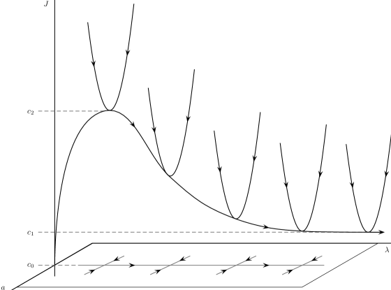
occurs up to a subsequence in time for every flow line. In cases (i) or (ii) we say, that tends to leave the variational space or escapes to infinity, see Figure 1 for an illustration. While (i) may occur in case of the two dimensional analogon to the prescribed scalar curvature problem, i.e. the Gaussian one, in our setting (i) is ruled out, as is bounded. However, since energy is decreased, and by virtue of (1.14) every flow line constitutes up to a subsequence in time a Palais-Smale sequence.
-
(i)
-
(2)
on the other hand an analysis of arbitrary Palais-Smale sequences shows, that
up to a subsequence in time eventually, where among other properties
-
()
either is a solution or and
-
()
is a vanishing perturbation
-
()
and weakly.
Note, that in case and only in case we have
since on by definition. In other words is of zero weak limit type and tends to leave the variational space , i.e. escapes to infinity, via
(1.15) up to a subsequence in time at least.
-
()
-
(3)
based on an energy consumption argument relying on lower bound estimates on , if
up to a subsequence in time, then also eventually, i.e. for , and
This is to say, that does not only escape to infinity, but also becomes critical at infinity. A priori however this does not imply a unique limiting profile of type (1.15) for .
Remark 1.1.
In any case different flows may produce along their respective flow lines non coinciding sets of end configurations as in (1.15). For instance, as a pathological example in [20] shows, while the strong gradient flow exhibits zero weak limit non compact flow lines escaping to infinity, all of which have one and the same end configuration for , a slight variation of this flow is compact, i.e. is convergent or in other words does not have any flow lines escaping to infinity at all.
In order to avoid such issues we will
-
(i)
define an energy decreasing flow as in (1.13).
-
(ii)
prove beyond (3) above, that every zero weak limit flow line of escaping to infinity, i.e.
has a unique end configuration, informally
and is a Dirac measure for .
- (iii)
- (iv)
-
(v)
show, that none of these end configurations can be avoided as an obstacle to energetic deformation, i.e. they are critical points at infinity, cf. Definition 2.6.
Whereas (i)-(iii) are seen by analysing one specific flow , the index in (iv) is justified from the subcritical approximation, while the minimality condition (v) follows from a Morse lemma at infinity, i.e. a faithful expansion of on of Morse type. And this is, how to prove Theorem 2.
Theorem 2 as a result, in particular and foremost the exclusion of tower bubbles along a suitable flow, is not new, we refer to Appendix 2 in [3] for the case of the sphere. While in the latter work the most important arguments are nicely displayed, there is an inaccuracy, which we shall discuss after the proof of Theorem 2 at the end of this work, whose motivation besides is threefold
- (1)
-
(2)
the flow, we study, is in contrast to previous explicit constructions, cf. [2],[3],[5],[6],[7], norm and positivity preserving, hence provides a natural deformation of energy sublevels as subsets of the variational space for the variational functional on . Conversely these properties hold true for Yamabe type, i.e. weak -pseudo gradient flows, cf. [8],[18],[17], whose analysis relies on higher curvature norm controls, hence are not easy to adapt at infinity to exclude tower bubbles.
-
(3)
the construction of the flow as in Section 4 is explicit and keeps track of all the relevant quantities. In particular we move the blow-up points exactly along the stable manifolds of , which will prove helpful for adaptations to describe the flow outside , but still in a concentrated regime.
2 Critical points at infinity
While (i)-(v) above identify the critical points at infinity according to [1], their definition as in [1] is related to a pseudo gradient or more generally to a flow of type (1.13). And therefore this notion of a critical point at infinity is not intrinsic to the variational problem. On the other hand in some situations, cf. [20] and Remark 1.1, it is counter intuitive to identify a critical point at infinity with a non compact flow line of a specific flow, if any non compactness can be avoided by considering a different flow.
We wish to take a different view. Let us first define various objects related to Palais-Smale sequences. Strictly speaking Proposition 3.1 and Remark 3.1 describe the possible Palais-Smale end configurations as elements of (2.1) below, but in fact each such configuration can be easily obtained as a natural limit of a Palais-Smale sequences.
Definition 2.1.
Let denote the blow-up profiles arising from Palais-Smale sequences on , i.e.
| (2.1) |
We also
-
(i)
denote for by
the blow-up profiles arising from Palais-Smale sequences in .
-
(ii)
denote for with corresponding , cf. (2.1), by
(2.2) the unique limiting energy of any Palais-Smale sequence with as limiting profile.
-
(iii)
call for an open set an open neighbourhood of , if
and call an open set an open neighbourhood of , if
-
(iv)
call open, if
and closed, if is open.
Remark 2.1.
We remark, that
-
(i)
as a fundamental property
(2.3) cf. (2.2), i.e. for any with and up to a subsequence
in the sense of distributions. In fact by (3.7) the number of diracs is bounded. And either up to a subsequence or by (3.7) and (3.8) the sequence of solutions constitutes a Palais-Smale sequence of bounded norm and energy, whence Proposition (3.1) is applicable.
-
(ii)
finite intersections and arbitrary unions of open subsets of are again open.
-
(iii)
for and
is a natural neighbourhood of in .
In this way the Palais-Smale closure of , i.e. with the topology
becomes a separable Hausdorff space and we identify a neighbourhood of with its part in the variational space , cf. (iii) in Definition 2.1.
Definition 2.2.
Let
denote the set of consecutive, energy decreasing deformations , for which
-
(1)
as in (1.13)
-
(2)
Lipschitz
-
(3)
during we deform along
i.e. solving for consecutively the initial value problems
-
(4)
and finally
i.e. solving the initial value problems
Note, that every acts as a family of diffeomorphisms and along each flow line there holds almost always and, cf. (1.13),
Since ultimately critical points at infinity will be related to an obstacle to energetic deformation below a certain energy , we introduce the subsequent notions.
Definition 2.3.
For we call a closed subset -reducible, if
Clearly every closed subset of a -reducible set is -reducible, is -reducible and, if is -reducible and , then is -reducible as well.
Definition 2.4.
For we call a closed subset -capturing, if
To clarify this definition
-
(i)
consider the case, that is -capturing. Then clearly as an energy level is not an obstacle to energetic deformation.
-
(ii)
consider with the stretched maximum
In this case is -capturing, while no subset of is -capturing. In fact suppose, that some was -capturing. Then there exists and
-
(1)
such, that , since is closed.
-
(2)
some such, that for every -reducible we find such, that
Combining then with a flow , along which for
to a flow , we then find while this is readily impossible, when choosing
-
(1)
-
(iii)
consider the function as in Figure 2 and observe, that
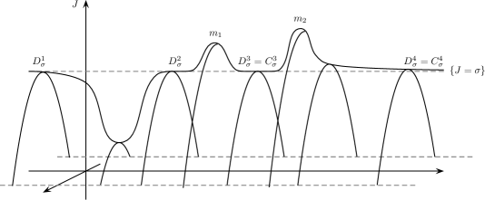
Figure 2: Some function on -
(1)
every -reducible , which by definition is closed, is a subset of some complement
-
(2)
evidently and for every and sufficiently small we may deform every -reducible along some onto , i.e. is -capturing.
-
(3)
we may deform along some suitably small neighbourhoods of in such a way, that leaves invariant, while for some
-
(4)
as a consequence also is -capturing.
-
(5)
in fact is minimal in the sense, that is -capturing and for every -capturing also is -capturing, cf. Definition 2.5.
We remark, that any flow, by which we push a neighbourhood of below a certain energy , requires diverging speed towards , cf. (i) of Remark 2.2. A possible choice is near
-
(1)
While the set in the aforegoing examples is naturally critical, the set is the one of variational interest, i.e. the obstacle to energetic deformation, and correctly identified as the unique and minimal strongly critical set as defined below.
Definition 2.5.
We call strongly critical, if is -capturing and
Note, that this definition does not exclude the case, that is strongly critical. But if so, the situation is variationally trivial.
Proposition 2.1.
is strongly -critical.
Proof.
Let and arbitrary. Then using (2.3)
and we consider for some open subneighbourhoods of satisfying
Let such, that Note, that to travel a distance along a negative gradient flow line
comes at an energetic cost , since
We therefore consider some arbitrary -reducible and choose such, that
and given by during and the negative gradient flow for . We then show
in order to verify, that is -capturing. Hence consider some
as an initial data for the negative gradient flow line . Then
-
(i)
in case , the flow line can never reach , since otherwise would have to travel through bridging a distance , which comes at an energetic cost , while we have only an energetic gap of at disposition. As a consequence enters and does so in some finite time , which is uniformly upper bounded for all .
-
(ii)
in case and by the same argument as above, the flow line can never reach and thus enters in some uniformly upper bounded time .
-
(iii)
in case , then the flow line can never leave again by energy consumption.
As a consequence for we find
Recalling , this shows, that is -capturing. To prove, that is even strongly -critical, we consider some arbitrary -capturing and show, that is also -capturing. Again this follows from energy consumption flowing by the negative gradient flow away from . ∎
Proposition 2.2.
There exists a minimal, strongly critical .
Proof.
We may assume, that is not strongly critical. In particular and necessarily since otherwise for some by (2.3)
and this implies, that every -reducible can be brought down into for any in finite time along the negative gradient flow. Hence and by virtue of Proposition 2.1 we may consider
as a by inclusion partially ordered set. Let us denote by an arbitrary chain in . Then the assertion follows from Zorn’s Lemma, provided
is strongly critical, i.e. a lower bound for this chain in . To see the latter we have to show, that
-
(i)
is -capturing and
-
(ii)
is -capturing, whenever some is -capturing.
To prove (i) consider an arbitrary . Then, as is closed and is sequentially compact, cf. (2.3), there exists such, that is a neighbourhood of . Moreover, since is strongly critical, is in particular -capturing. Hence according to Definition 2.4 we find , such that we may capture every -reducible in by some as desired. Therefore and, since is arbitrary, is -capturing itself.
To prove (ii) consider an arbitrary -capturing . Since is strongly critical, by definition is -capturing for every . Arguing as for (i) we then find, that is -capturing as well. ∎
While Zorn’s Lemma, as we have seen, guarantees the existence of minimal strongly -critical sets, we have to show uniqueness of the latter separately.
Lemma 2.1.
There exists a unique, minimal strongly critical .
Proof.
By Proposition 2.2 there exists some minimal, strongly critical . Suppose, there exists another minimal strongly critical .
Then, since is strongly -critical, is by definition -capturing. And, since is strongly critical, we deduce, that is -capturing as well.
Moreover consider some arbitrary -capturing . Then, since is strongly critical, also is -capturing. And, since is strongly critical, also is -capturing.
We conclude, that is strongly critical, which contradicts the minimality of and . ∎
With Lemma 2.1 at hand we then define critical points at infinity as follows.
Definition 2.6.
We call a critical point at infinity, if .
Note, that the definition of does only depend on and the space of admissible deformations, in particular does not depend on a specific flow or for instance a presumed Morse structure around elements of .
Let us show, that the unique, minimal strongly critical sets are generically meaningful.
Proposition 2.3.
Let be a non degenerate critical point of finite index. Then .
Proof.
Arguing by contradiction, we suppose . Then
Consider in a Morse chart around , e.g.
a sequence
to which for arbitrarily small we attach -dimensional disks
with boundary Then for degree reasons, see below,
| (2.4) |
However, since each is -reducible and is -capturing, by definition we find
| (2.5) |
for suitable and . Then (2.4) and (2.5) lead to the obvious contradiction
Hence we are left with proving (2.4). On the Morse chart consider the continuous map
with denoting the natural identification of the disk via
with the sphere with south pole . After rescaling we hence obtain a continuous map
Moreover for and recalling we have
whence we may assume
Consequently and with denoting the north pole of
whence we may extend continuously and restrict by putting
| (2.6) |
We also find, that for all sufficiently large
| (2.7) |
for any flow . In fact let Then by construction
Let and suppose for some . Then by (2.6) necessarily and
leading to a contradiction for sufficiently large. Then (2.7) implies, that for the natural embedding
and for every the composition factorizes to a map
Since as a homotopy equivalence, and by continuity and constancy of the degree on
Consequently From this (2.4) readily follows. ∎
Analogous arguments then show, that a finite index Morse structure at infinity leads to the same conclusion. The spaces following are real Banach.
Lemma 2.2.
Let and suppose, that for a neighbourhood of we may parameterise
-
(i)
with spaces and a neighbourhood of
-
(ii)
open with spaces and
-
(iii)
Then
-
(1)
-
(2)
Proof.
As for (1) suppose . We then decrease energy within via
-
decreasing and until to find
-
increasing until to find
-
decreasing until to find
Hence and by minimality of necessarily , proving (1). (2) then follows exactly as Proposition 2.3 upon replacing by and by . ∎
Let us comment on these Morse structure results.
Remark 2.2.
-
(i)
Suppose, that as in Lemma 2.2 on a neighbourhood of we have a diffeomorphism
such, that the functional takes form
Since corresponds to the Palais-Smale limit, clearly
But evidently for
As a consequence must be degenerating and, while has a clear Morse structure at infinity, its derivative will not relate in a trivial way to that of the Morse representation. For instance consider
for and the functional , which expands as
The tangential space is given by whence for the derivative
In particular for every . On the other hand has under (1.5) readily a Morse structure for and .
- (ii)
-
(iii)
Concerning the infinite index case, consider for instance the functional
Then . In fact either or , since necessarily . If , then by definition and with
In particular for all times is impossible, whence there exists such, that
Let and compute We then find
Hence for sufficiently small the energy is increasing along for a short time. This of course contradicts (1.13), since .
-
(iv)
The case in Lemma 2.2 and hence the question, whether or not a critical point at infinity can have an infinite index, is more delicate. For instance does for
represent an obstacle to energetic deformation, i.e. for any energy decreasing flow of type ? We conjecture, that the answer is no. In any case infinite indices do not occur in our framework.
We finally characterize as an obstacle to energetic deformation as follows.
Proposition 2.4.
Let . Then every -reducible is also -reducible, if and only if
Proof.
The case trivially holds true. Hence let .
Suppose, that every -reducible is also -reducible. Since for trivially every -reducible is also -reducible, we find, that every -reducible is also -reducible. Consider hence for an arbitrary -reducible and choose such, that . Since is also -reducible, we find and such, that , cf. Definition 2.3. As a consequence and, since , the empty set is -capturing, cf. Definition 2.4, and then trivially strongly -critical as well, cf. Definition 2.5. By uniqueness of a minimal, strongly -critical we conclude .
Vice versa suppose, that and consider
In view of Definition 2.3 we then have to show . Arguing by contradiction we assume and find, that every -reducible is also -reducible. Since is strongly -critical and by Definition (2.5) also -capturing, we find and for every -reducible some and such, that . But this implies, that every -reducible is also -reducible and therefore every -reducible is also -reducible. This contradicts the minimality of leading to the desired contradiction. ∎
From Proposition 2.4 we recover the classical deformation lemma.
Lemma 2.3.
Let and suppose, that
Then as a weak deformation retract.
3 Preliminaries
Let us start with a quantification of the deficit for some from solving (1.2).
Lemma 3.1.
There holds More precisely on a geodesic ball for small
where . In particular
-
(i)
-
(ii)
-
(iii)
The expansions stated above persist upon taking and derivatives.
Proof.
Cf. Lemma LABEL:I-lem_emergence_of_the_regular_part in [14]. ∎
Thereby we may describe the blow-up behaviour of Palais-Smale sequences for (1.4).
Proposition 3.1.
Let be a sequence with and satisfying
| (3.1) |
for some . Then up to a subsequence there exist
and for sequences
for some such, that and
| (3.2) |
and for each pair there holds
| (3.3) |
Proof.
Cf. Proposition LABEL:I-blow_up_analysis in [14]. ∎
Remark 3.1.
We remark, that
- (i)
- (ii)
- (iii)
- (iv)
Proposition 3.1 justifies to consider the following subset of peaked function and look for zero weak limit Palais-Smale sequences thereon only.
Definition 3.1.
For and let
-
(i)
-
(ii)
However, for a precise analysis of on it is convenient to make the representation of its elements unique.
Proposition 3.2.
For every there exists such, that for with
admits a unique minimizer depending smoothly on and we set
| (3.9) |
Proof.
Cf. Appendix A in [4]. ∎
For the sake of brevity and recalling (1.3) we denote e.g.
for a set of points and for and we let
-
(i)
and
-
(ii)
-
(iii)
in particular pointwise, i.e.
With this notation the term
from Proposition 3.2 is orthogonal to with respect to the scalar product
and we define for its complement
A precise analysis of on was performed in [14] by testing the variation separately with the bubbles and their derivatives on the one hand and orthogonally to them, i.e. with elements of on the other.
Recalling (3.3) we collect below some principal interactions over various integrals involving , which clearly appear in the gradient testing or expansion of the energy itself. Note, that .
Lemma 3.2.
For and and we have with constants
-
(i)
-
(ii)
-
(iii)
for
-
(iv)
for and for
-
(v)
for
-
(vi)
-
(vii)
.
Let us comment on the following lemmata, which describe the testing of . First a testing in an orthogonal direction is due to orthogonalities small.
Lemma 3.3.
For with and there holds
In combination with the well known uniform positivity of the second variation on the orthogonal space , cf. [22], this allows us to estimate itself in terms of the aforegoing quantities.
Lemma 3.4.
For with and is as in (3.9) there holds
The latter smallness estimate will turn out to be sufficient to consider as a negligible quantity in the sense, that is not responsible for a blow-up.
Let us turn to the testing in the directions of the bubbles and their derivative as had been performed carefully in low dimensions in Section 4 of [18]. We note, that for each bubble we have three quantities associated, namely and . The -direction then corresponds to a testing with a bubble itself, since . Again for the sake of brevity let us define the quantities
| (3.10) |
which are the principal terms in the nominator and denominator of , cf. (1.4).
Lemma 3.5.
For and sufficiently small the three quantities , , can be written as
with positive constants and up to some In particular
Proof.
Evidently the principal term due to largeness of the concentration parameters and smallness of the interaction terms in the above expansion is the one related to forcing into a certain regime.
Lemma 3.6.
For and sufficiently small the three quantities , and can be written as
with positive constants and up to some
Proof.
Here at least in high dimensions the principal terms are the ones related to and . The first one turns out to be responsible for a potential diverging flow line within depending on the sign of , the latter one, measuring interactions, may be relatively strong or weak depending on, whether the corresponding are close to or not. In any case these interaction terms will turn out to be responsible for excluding tower bubbling, i.e. multiple bubbles concentrating at the same point along a flow line, just as they prevent tower bubbling in the subcritical case, cf. [15]. The location of a bubble on in the sense of the centre is principally determined from the -testing below.
Lemma 3.7.
For and sufficiently small the three quantities , and can be written as
with positive constants and up to some
Proof.
Evidently the principal terms are the one related to , trying to force the centres of concentration to be close to critical points of , and the one related to .
Of course the source of delicacy is, that the principle terms above are related by their error terms.
Proposition 3.3.
For sufficiently small there holds uniformly on
Proof.
Here and later on we use for two functions the shorthand notation
We note, that the latter gradient estimates evidently prevent the existence of a solution in and allow us to compare the quantities appearing to and vice versa. Finally we may perform an expansion of the energy itself on , which reads as
Lemma 3.8.
For and , both and can be written as
with positive constants and up to some
Proof.
In the following we will work with the normalisation to the unit sphere, i.e. on , whereas in [14] and [15] we have been restricting to , i.e. to the unit sphere with respect to the conformal -volume, cf. (1.4). However, along an energy decreasing flow line we have
thanks to the positivity of the Yamabe invariant, cf. (1.1), and hence a control of via and vice versa. Moreover on there holds
cf. (3.10), whence, as an easy computation shows, we have uniform energy control on each via
In particular the aforegoing Lemmata are still applicable, when working on instead of .
4 Flow construction
Lemma 4.1.
For bounded and
there exist with
-
(i)
-
(ii)
such, that moving along
there holds
Remark 4.1.
Lemma 4.1 simply tells us, that for every principal movement
we may
-
(i)
preserve the movement of along
-
(ii)
modify the movement of along only slightly by such, that we
-
(iii)
ensure, that writing
remains compatible with the representation on in the sense of proposition 3.2 and
-
(iv)
preserve the norm of .
Proof.
Let us suppose a orthogonality preserving evolution
exists. Then the preservation of orthogonality, i.e. for , necessitates
-
(i)
in the -variable
-
(ii)
in the -variable
-
(iii)
in the -variable
Since pointwise and, as follows from Lemmata 3.1 and 3.2,
we may choose some dual to such, that
| (4.1) |
We then may solve - via and for
| (4.2) |
Conversely solving with the above choice of we find
Hence the statement on follows. Therefore and in particular due to we find as well
where , whence is equivalent to putting
noticing that on . ∎
Definition 4.1.
Let . Then for arbitrary constants
| (4.3) |
consider on the subsets
-
(i)
-
(ii)
-
(iii)
-
(iv)
-
(v)
and to each of these subsets a corresponding cut-off functions
satisfying
Moreover for some monotone cut-off function with
define
As set out in Lemma 4.1 we then evolve on according to
with a constant , i.e.
where
| (4.4) |
Remark 4.2.
- (i)
- (ii)
-
(iii)
Whereas the movement in and are obviously well defined, we note, that
whence by non degeneracy, cf. (1.5), also the movement in is well defined.
-
(iv)
The union covers for sufficiently small. Indeed we have
on , whence , a contradiction for .
-
(v)
In view of Lemmata 3.5, 3.6 and 3.7 we call
-
()
-
()
-
(a)
the principal terms in and . The flow is designed in such a way, that whenever the principal terms are dominant in the expansion of the lemmata above, their corresponding movement in and will decrease energy. Notably we move as little as possible by the Laplacian of .
-
()
Lemma 4.2.
On the evolution
for a cut-off function satisfying
induces a semi-flow
i.e. the flow exists for all times, remains non negative and preserves , provided
cf. (4.3).
Proof.
Since is the -gradient, we may write and is a locally smooth vectorfield on . So we have short time existence and due to
as on by construction and
by scaling invariance of , the -norm is preserved. Moreover, as Proposition 4.1 will show, there holds whence in combination with the positivity of the Yamabe invariant we have
| (4.6) |
along each flow line for its time of existence. Hence and thus are uniformly bounded along each flow line and, as is easy to see, locally smooth. Therefore every flow line exists for all times. Moreover, as , we find from (4.4), (4.5) and (ii) of Lemma 4.1, that
provided , i.e. is sufficiently large. Hence
by definition of the -gradient and positivity of . We conclude using (4.6), so every initially non negative or positive flow line becomes or remains positive for all times to come. ∎
We point out, that the long time existence part is not critical, since the flow is based on a strong gradient, i.e. the gradient corresponding to the metric on the variational space, and thus falls into the class of ordinary differential equations, cf. [4] or [7], in contrast to Yamabe type flows as in [8] or [18].
Proposition 4.1.
Proof.
First consider the flow on for some . We then have
whence by virtue of Lemmata 3.6, 3.7 and Proposition 3.3
and thus
Moreover by the well known positivity of on we find by expansion
| (4.7) |
where we made use of Lemma 3.3. Hence
| (4.8) |
Secondly for
we have due to by scaling invariance of and due to (4.5), (4.7)
Moreover Lemma 3.5 and Proposition 3.3 show
and we obtain
| (4.9) |
Therefore combining (4.8) and (4.9)
and recalling the definitions of and from Definition 4.1 we conclude
| (4.10) |
We turn to the and evolution. By Proposition 3.3 and the definitions of and we find up to some
from Lemma 3.6 the relation
and likewise from Lemma 3.7
Thus recalling of Remark 4.2 and the definition of we have for some positive constants
| (4.11) |
up to some . Let us now suppose
In particular we may assume , cf. Definition 4.1, and this implies
We thus infer from (4.11), that up to some
and with possibly different constants
| (4.12) |
recalling the definition of , cf. Definition 4.1, for the last inequality. Note, that
| (4.13) |
cf. (3.3), and recalling Definition 4.1, there holds
-
(i)
for
-
(ii)
for .
Therefore
and, since , cf. Definition 4.1, plugging this into (4.12) we conclude
| (4.14) |
provided . We now assume contrarily and in addition
Then from (4.11) and recalling the definition of we find with possibly different constants
up to some . Note, that
and in particular . Hence up to the same error as above
Recalling Definition 4.1 there holds
and in the latter case , i.e. . Hence we deduce, that in any case
and (4.14) follows again, provided is sufficiently large. We finally consider the remaining case
Then recalling again the definition of we find from (4.11)
up to some
Let us decompose for some and with a slight abuse of notation
In particular for we have
Hence, if for were close to the same critical point, we find, cf. 3.3, the contradiction
Hence for we may assume, that are close to different critical points of , whence
Moreover for
Consequently
up to some
and rearranging this we obtain up to the same error
Recalling (4.13) and from Definition 4.1
-
(i)
for
-
(ii)
for ,
we find
and using for and
Therefore and recalling for
up to some
Consequently (4.14) follows again and thus in any case from and upon choosing
We therefore conclude combining (4.10) and (4.14), that on for sufficiently small
which recalling the definitions of , cf. Definition 4.1 simplifies to
| (4.15) |
As for the gluing with the gradient flow on some via , i.e.
we remark, that with a suitably small constant from (4.15) we now have
on , but also
due to Proposition 3.3 and Lemma 3.4. Thence the proposition follows. ∎
Let us show, that a flow line, which at least up to a sequence in time concentrates for some eventually for every in , then the whole flow line will eventually stay for every in . In particular such a flow line will be eventually governed by the prescribed movements and as in Definition 4.1, i.e. the patching with the gradient flow will be irrelevant.
Lemma 4.3.
If for a flow line
then for every there exists such, that
Proof.
If the statement was false, there would exist such, that
for some arbitrarily small . Thus the flow has during to travel a distance
with bounded speed and energy decay due to proposition 4.1. So the time for this travelling is lower bounded, i.e. , and thus we consume at least a quantity of energy
Clearly this leads to a contradiction, as the lower bounded energy is never increased. ∎
5 Non compact flow lines
Since every flow line can be considered as a Palais-Smale sequence, when restricted to a sequence in time, every non compact zero weak limit flow line has by Proposition 3.1 to enter every and by lemma 4.3 to remain therein eventually. Let us study such a flow line , which then satisfies
-
()
-
()
-
()
-
()
for all times to come. First note, that from we have , while from and
and finally from and (4.5), cf. also (3.10),
Recalling the definition of , cf. Definition 4.1, we then have for sufficiently large
and may thus assume, that eventually, hence from now on and for all times to come
| (5.1) |
We turn to describing the movement in and . Clearly we may assume
due to Lemma 4.3 and so at least for a time sequence
Hence and , cf. Definition 4.1, show, that necessarily
Since we assume to be Morse, we conclude, that at least for a sequence in time
On the other hand due to all move exclusively along the gradient of , whence necessarily
and has to move along the stable manifold of with respect to the positive gradient flow for , hence
But the only possibility for to increase is , cf. , whence necessarily as a first consequence
In particular we may assume from now on. Secondly, since for
cf. Definition 4.1, we derive from using and
whence for and we may therefore assume from now on
| (5.2) |
Thirdly, as we had said, has to grow at times , and then we have
| (5.3) |
whereas generally there holds due to and
where we used . Since is Morse and is close to and moves along , we have
| (5.4) |
and consequently
| (5.5) |
In particular (5.3) and (5.5) imply, that we may assume from now on and for all times to come
| (5.6) |
for some fixed . From (5.2) and (5.6) we then may exclude tower bubbling, i.e.
Indeed in the latter case
and , whence
a contradiction. Hence we may assume , thus and therefore
| (5.7) |
for all times to come due to , cf. (5.2). In particular and therefore simplifies to
due to (5.6), (5.7) and, cf. Definition 4.1, and
-
(i)
on ;
-
(ii)
on
We turn our attention to the movement in . Since we may assume by now , hence
cf. Definition 4.1, (5.6) and (5.7), and due to (4.5), we have
where we made use of . Note, that due to we have
up to some . Recalling (3.10) we then find, that up to some
there holds and secondly
i.e.
Hence we obtain up to the same error
Consequently we have
| (5.8) |
as long as due to and , cf. (5.4). Thence necessarily
| (5.9) |
for all times to come. Indeed we may assume
-
(i)
-
(ii)
with
We then find from (5.8), since on , that
as long as , and thus by virtue of (5.7)
Consequently and, since we may assume
provided is sufficiently large, we will stay in for all times, whence by virtue of (5.8)
a contradiction. We thus conclude from (5.2), , (5.6), (5.9) and (5.1), that eventually
for some . We have thus derived the non trivial part of
Proposition 5.1.
A zero weak limit flow line is non compact, if and only if eventually
-
(i)
decays exponentially and
-
(ii)
decays exponentially and
-
(iii)
increases exponentially and
-
(iv)
along exponentially fast, where
for all . Conversely flow lines satisfying - exist.
Proof.
By what we have seen above, every non compact zero weak limit flow line has to satisfy - above eventually and clearly every flow line satisfying - is non compact with zero weak limit. Hence we are left with showing their existence. Let us choose for simplicity as initial data
for and for . Recalling , cf. Lemma 4.1, we have
cf. and hence is preserved. Secondly due to also is preserved. Thirdly
follows from and , cf. , hence also is preserved. In particular
are preserved, as long as we do not leave some , upon which and are valid. Thus
due to . Since and for by assumption, there holds for
whence and , so . Hence the above will never be left and . ∎
Proof of Theorem 2.
Consider the flow introduced in Lemma 4.2, i.e.
which decreases the energy according to Proposition 4.1. Then by energy reasoning every flow line induces upon choice of a subsequence in time a Palais-Smale sequence . Indeed is by positivity of the Yamabe invariant strictly positive, while by virtue of Propositions 3.3 and 4.1 every flow line consumes energy as long as . Then Proposition 3.1 and the comment following it show, that upon a subsequence is of zero weak limit, if and only if concentrates in the sense
in which case is of zero weak limit itself, as Lemma 4.3 shows. Hence according to Proposition 5.1 the full flow line concentrates simply with limiting profile and energy
| (5.10) |
respectively, where is a dimensional constant and
are distinct. Hence zero weak limit sequences along a flow line are classified with respect to their end configuration, which corresponds one to one to subsets of on the one hand and to finite energy and zero weak limit subcritical blow-up solutions on the other, cf. [15]. And of course flow lines of the latter type do exist by Proposition 5.1.
So let us consider
and denote correspondingly by
the unique, zero weak limit subcritical blow-up solution from [15] of the same limiting profile and energy
Then by virtue of Proposition 3.1 in [15] there exists such, that for all for
i.e. uniqueness as a solution on some .

Hence
for some and any contains exactly one element as a subcritical solution with
as Morse index. And we have a homotopy equivalence by attaching a cell, cf. Figure 3,
along the unstable manifold of and suspended at with energy
Since due to Hölder’s inequality, we then find
for the -th relative singular homology with of the pair
see [11]. Thus we observe a change of topology of the sublevel sets of on
| (5.11) |
while thanks to Proposition 3.3 we know, that for sufficiently small
In other words this change of topology happens on (5.11) as a neighbourhood of the limiting profile (5.10) of a non compact, energy decreasing, zero weak limit flow line of . And in fact this limiting profile does correspond to a critical point at infinity, as exhibits a correct Morse structure on this neighbourhood, cf. Proposition 5.2 and Lemma 2.2. Hence we may justly
-
(i)
say, that this change of topology is induced by this critical point at infinity
-
(ii)
associate to this critical point at infinity the index
(5.12)
This completes the proof. ∎
To establish the Morse structure at infinity, we first require a further orthogonalization.
Lemma 5.1.
For every there exists a unique minimizer for
provided is sufficiently small, and, if for , there holds
Proof.
Clearly and we may represent every uniquely as
Then by construction
and by positivity of on and smallness of we find
| (5.14) |
which is to say, that the -direction is a positive, i.e. energy increasing one. Moreover
| (5.15) |
Proposition 5.2.
For for and sufficiently small there holds
for , where upon rescaling
-
(i)
-
(ii)
are local coordinates of in a Morse chart around , upon which
-
(iii)
are the eigenvectors negative eigenvalues of
Remark 5.1.
At this point, cf. (5.12), it is hardly surprising, that for the number of negative directions
Proof of Proposition 5.2.
We clearly have to study at only. From Proposition 5.1 in [14] we have
with positive constants , noting, that
-
(i)
there is no in the remainder in case
-
(ii)
and
-
(iii)
the blow-up points are far from each other, since
-
(iv)
and for , in particular
Moreover and, since , we obtain
recalling the non degeneracy assumption (1.5). Passing to the Morse charts and expanding we get
where . Finally consider the scaling invariant function
whose restriction to
reflects the restriction of to . Then has a unique, strict and non degenerate maximum in
In particular and due smallness of on necessarily
Denoting hence by for the eigenvector with negative eigenvalue of
and with , we conclude with
Let us conclude with a discussion of the inaccuracy in [3], namely, that the deformation constructed in its Appendix 2, cf. also [5], leaves the variational space
by not preserving non negativity and not preserving the normalisation . While the first violation is not an issue as exposed in [5], the latter has to be addressed. Let us discuss some possibilities.
-
(i)
Naive renormalisation The most simple approach would be to let flow and renormalise afterwards, which however might lead to a lack of well definedness as a flow on .
-
(ii)
Brute force normalisation The construction in [3] is an adaptation at infinity, i.e. flow lines of type
Leaving the -part aside, the constructed vectorfield prescribes a movement in and keeping the scaling parameters invariant. Hence one might adjust the dynamically, e.g. along
in order to preserve . This however adds error terms of type
when verifying energy decreasing, i.e. , and hence necessitates a dynamical control of these quantities, which is not available from [3] or [5]. We perform this argument here.
-
(iii)
Geometric normalisation The most intuitive way to adjust the vectorfield constructed in [3] in order to preserve is passing from to
(5.16) Of course the flow lines for and are then not evidently related and passing from to perturbs the movements in and . But then the statement of Proposition A2 in [3], that away from the critical points at infinity is non increasing, requires justification.
Since there has been a variety of scientific research relying on [3] and in particular its Appendix 2, we would like to point out, that in our opinion and based on the availability of better estimates on the errors induced by the necessity to normalise the flow are not critical at least in low dimensions . Also note, that for instance [2] describing the positivity and norm preserving gradient flow, is not affected.
Acknowledgment
M.Mayer has been supported by the Italian MIUR Department of Excellence grant CUP E83C18000100006.
References
- [1] Bahri A., Critical points at infinity in the variational calculus, Seminaire Equations aux derivees partielles (Polytechnique), (1985-1986), Talk no. 21, p. 1-31
- [2] Bahri A., Critical points at infinity in some variational problems, Research Notes in Mathematics, 182, Longman-Pitman, London, 1989.
- [3] Bahri A. An invariant for Yamabe type flows with applications to scalar curvature problems in higher dimensions, Duke Mathematical Journal, 81 (1996), 323-466.
- [4] Bahri A., Coron J.M., The Scalar-Curvature problem on the standard three-dimensional sphere, Journal of Functional Analysis, 95 (1991), 106-172.
- [5] Ben Ayed M., Chen Y., Chtioui H., Hammami M., On the prescribed scalar curvature problem on 4-manifolds, Duke Mathematical Journal, 84 (1996), 633-677.
- [6] Ben Ayed M., Chtioui H., Hammami M., The scalar-curvature problem on higher-dimensional spheres. Duke Math. J. 93 (1998), no. 2, 379-424.
- [7] Ben Ayed, M.,Ould Ahmedou, M., Multiplicity results for the prescribed scalar curvature on low spheres, Ann. Scuola Norm. Sup. Pisa Cl. Sci. (5) Vol. VII (2008), 1-26
- [8] Brendle, S., Convergence of the Yamabe flow for arbitrary initial energy, J. Differential Geom. 69 (2005), no. 2, 217–278.
- [9] Brezis, H., Nirenberg, L., Positive solutions of nonlinear elliptic equations involving critical sobolev exponents, Communications on pure and applied mathematics , 1983, Vol.36(4), p.437-477
- [10] Chang S. A., Yang P., Prescribing Gaussian curvature on , Acta Math. Volume 159 (1987), 215-259.
- [11] Chang K.C., Infinite-dimensional Morse theory and multiple solution problems. Progress in Nonlinear Differential Equations and their Applications, 6. Birkhäuser Boston, 1993.
- [12] Lee J., Parker T., The Yamabe problem. Bull. Amer. Math. Soc. (N.S.) 17 (1987), no. 1, 37-91.
- [13] Li Y.Y., Prescribing scalar curvature on and related topics, Part II, Existence and compactness. Comm. Pure Appl. Math. 49 (1996), 437-477.
- [14] Malchiodi A., Mayer M., Prescribing Morse scalar curvatures: blow-up analysis. International Mathematics Research Notices,2020/02, rnaa021
- [15] Malchiodi A., Mayer M., Prescribing Morse scalar curvatures: subcritical blowing-up solutions. Journal of Differential Equations, Volume 268, Issue 5, Pages 2089-2124
- [16] Malchiodi A., Mayer M., Prescribing Morse scalar curvatures: pinching and Morse theory. To appear in Communications in Pure and Applied Mathematics
- [17] Malchiodi, A., Struwe, M., Q-curvature flow on , Journal of Differential Geometry 73, 1-44
- [18] Mayer M., A scalar curvature flow in low dimensions. Calc. Var. Partial Differential Equations 56 (2017), no. 2, Art. 24, 41 pp
- [19] Mayer M., Prescribing Morse scalar curvatures: incompatibility of non existence. To appear
- [20] Mayer M., Prescribing scalar curvatures: non compactness versus critical points at infinity. Geometric Flows, 4(1), pp. 51-82
- [21] Mayer, Martin; Ndiaye, Cheikh Birahim. Barycenter technique and the Riemann mapping problem of Cherrier-Escobar. J. Differential Geom. 107 (2017), no. 3, 519-560
- [22] Rey, O. The role of the Green’s function in a non-linear elliptic equation involving the critical Sobolev exponent, Journal of Functional Analysis Volume 89, Issue 1
- [23] Schoen, R., Conformal deformation of a Riemannian metric to constant scalar curvature, Journal of Differential Geometry, Volume 20, Number 2 (1984), 479-495