A note on $h$-convex functions

Abstract.

In this work, we discuss the continuity of $h$-convex functions by introducing the concepts of $h$-convex curves ($h$-cord). Geometric interpretation of $h$-convexity is given. The fact that for a $h$-continuous function $f$, is being $h$-convex if and only if is $h$-midconvex is proved. Generally, we prove that if $f$ is $h$-convex then $f$ is $h$-continuous. A discussion regarding derivative characterization of $h$-convexity is also proposed.

1. Introduction

Let $I$ be a real interval. A function $f:I\to\mathbb{R}$ is called convex iff

(1.1) $$f\left({t\alpha+\left(1-t\right)\beta}\right)\leq tf\left({\alpha}\right)+\left(1-t\right)f\left({\beta}\right),$$

for all points $\alpha,\beta\in I$ and all $t\in[0,1]$. If $-f$ is convex then we say that $f$ is concave. Moreover, if $f$ is both convex and concave, then $f$ is said to be affine.

In 1979, Breckner [3] introduced the class of $s$-convex functions (in the second sense), as follows:

Definition 1.

Let $I\subseteq\left[0,\infty\right)$ and $s\in(0,1]$, a function $f:I\to\left[0,\infty\right)$ is $s$-convex function or that $f$ belongs to the class $K^{2}_{s}\left(I\right)$ if for all $x,y\in I$ and $t?\in[0,1]$ we have

$$f\left(tx+\left(1-t\right)y\right)\leq t^{s}f\left(x\right)+\left(1-t\right)^{s}f\left(y\right).$$

In the last years, among others, the notion of $s$-convex functions is discriminated and starred. In literature a few papers devoted to study this type of convexity. The building theories of $s$-convexity as geometric and analytic tools are still under consideration, development and examine. Due to Hudzik and Maligranda (1994), two senses of $s$-convexity $(0<s\leq 1)$ of real-valued functions are known in the literature, and given below:

Definition 2.

A function $f:\mathbb{R}_{+}\to\mathbb{R}$, where $\mathbb{R}_{+}=\left[{0,\infty}\right)$, is said to be $s$-convex in the first sense if

(1.2) $$f\left({\alpha x+\beta y}\right)\leq\alpha^{s}f\left(x\right)+{\beta}^{s}f\left(y\right)$$

for all $x,y\in\left[{0,\infty}\right)$, $\alpha,\beta\geq 0$ with $\alpha^{s}+\beta^{s}=1$ and for some fixed $s\in\left({0,1}\right]$. This class of functions is denoted by $K_{s}^{1}$.

This definition of $s$-convexity, for so called $\varphi$-functions, was introduced by Orlicz in 1961 and was used in the theory of Orlicz spaces. A function $f:\mathbb{R}_{+}\to\mathbb{R}_{+}$ is said to be a $\varphi$-function if $f(0)=0$ and $f$ is nondecreasing and continuous. The symbol $\varphi$ stands for an Orlicz function, i.e., $\varphi$ is defined on the real line $\mathbb{R}$ with values in $[0,+\infty]$ and is convex, even, vanishing and continuous at zero. For further details see [15], [17] ,[18],[32].

In fact, Breckner [3] walked in the footsteps of Orlicz’s definition (Definition 2) and introduced another type of $s$-convexity or what so called Breckner $s$-convex, as follows:

Definition 3.

A function $f:\mathbb{R}^{+}\to\mathbb{R}$, where $\mathbb{R}^{+}=\left[{0,\infty}\right)$, is said to be $s$–convex in the second sense if

(1.3) $$f\left({\alpha x+\beta y}\right)\leq\alpha^{s}f\left(x\right)+{\beta}^{s}f\left(y\right)$$

for all $x,y\in\left[{0,\infty}\right)$, $\alpha,\beta\geq 0$ with $\alpha+\beta=1$ and for some fixed $s\in\left({0,1}\right]$. This class of functions is denoted by $K_{s}^{2}$.

Remark 1.

We note that, it can be easily seen that for $s=1$, $s$-convexity (in both senses) reduces to the ordinary convexity of functions defined on $\left[{0,\infty}\right)$.

In general, a real-valued function $f$ defined on an open convex subset $C$ of a linear space is called Breckner $s$-convex if 1.3 holds for every $x,y\in C$, $\alpha,\beta\in[0,1]$ with $\alpha+\beta=1$, where $s\in(0,1)$ is fixed. More preciously, Breckner considered an open convex subset $\mathbb{M}$ of a linear space $\mathbb{L}$ and defined $f:\mathbb{M}\subseteq\mathbb{L}\to\mathbb{R}$, to be $s$-convex if 1.3 holds, for all $x,y\in\mathbb{M}$, $\alpha,\beta\in[0,1]$ with $\alpha+\beta=1$, where $s\in(0,1)$ is fixed. Also, Breckner considered a special case of $s$-convex functions which is so called rational $s$-convex, that is for all rational $\alpha,\beta\in[0,1]$ with $\alpha+\beta=1$ and points $x,y\in\mathbb{M}$, the inequality 1.3 holds. Furthermore, Breckner proved that for locally bounded above $s$-convex functions defined on open subsets of linear topological spaces are continuous and nonnegative.

In 1978, Breckner and Orbán [4] considered functions from a convex subset of a real or complex Hausdorff topological linear space of dimension greater than 1 into an ordered topological linear space such that all its order-bounded subsets are bounded, and showed that Breckner $s$-convex functions with $s\in(0,1]$ are continuous on the interior of their domain.

In 1994, Breckner [5] (see also [6]) proved that for a rationally $s$-convex function continuity and local $s$-Hölder continuity are equivalent at each interior point of the domain of definition of the function. Furthermore, it is shown that a rationally $s$-convex function which is bounded on a nonempty open convex set is $s$-Hölder continuous on every compact subset of this set. Indeed, Breckner [2], showed that if a real-valued function defined on a convex subset of a linear space endowed with topology generated by a direct pseudonorm is continuous and rationally Breckner $s$-convex for an $s\in(0,1]$, then it is locally $s$-Hölder.

In 1994, Hudzik and Maligranda [15], realized the importance and undertook a systematic study of $s$-convex functions in both sense. They compared the notion of Breckner $s$-convexity with a similar one of [18]. A function $f$ is Orlicz $s$-convex if the inequality (1.2) is satisfied for all $\alpha,\beta$ such that $\alpha^{s}+\beta^{s}=1$. Hudzik and Maligranda, among others, gave an example of a non-continuous Orlicz $s$-convex function, which is not Breckner $s$-convex.

In 2001, Pycia [24] established a direct proof of Breckner’s result that Breckner $s$-convex real-valued functions on finite dimensional normed spaces are locally $s$-Hölder. The same result was proved in [1] where different context was considered. For the same result regarding convexity see [7] and [8].

In the 2008, Pinheiro [25] studied the class of $K_{s}^{1}$ of $s$-convex functions and explained why the first $s$-convexity sense was abandoned by the literature in the field. In fact, Pinheiro , proposed some criticisms to the current way of presenting the definition of $s$-convex functions. We may summarize Pinheiro criticisms in the following points:

1. What is the ‘true’ difference between convex and $s$-convex in both senses.

2. So far, Pinheiro did not find references, in the literature, to the geometry of an $s$-convex function, what, once more, makes it less clear to understand the difference between an $s$-convex and a convex function whilst there are clear references to the geometry of the convex functions.

In the same paper [25], Pinheiro revised the class of $s$–convexity in the first sense. In [26], Pinheiro proposed a geometric interpretation for this type of functions.

Definition 4.

Let $U$ be any subset of $[0,\infty)$. A function $f:X\to\mathbb{R}$, is said to be $s$–convex in the first sense if

(1.4) $$f\left({\lambda x+\left({1-\lambda^{s}}\right)^{1/s}y}\right)\leq\lambda^{s}f\left(x\right)+\left({1-\lambda^{s}}\right)f\left(y\right)$$

for all $x,y\in U$ and $\lambda\in[0,1]$.

The presented reason from Pinheiro to why $s$-convexity in the first sense got abandoned in the literature, is that, if one takes $x=y=\frac{1}{4}$ with $\alpha=\frac{1}{2}$ and $\beta=1$ for example, one gets that $\alpha x+\beta y=0.125+0.25=0.375$. So that, if $s=\frac{1}{2}$, then the value of $\alpha x+\beta y$ would lie outside of the interval $[x,y]$, on the contrary of this, the value of $\alpha x+\beta y$ would lie inside of the interval $[x,y]$ in case of convexity. With this the first sense of $s$-convexity becomes a close to the meaning of convexity and so the geometric explanation of $s$-convex function is easy to be compared with the geometry of convex function if some further restrictions are imposed to it.

The proposed geometric description for $s$-convex curve in the first sense stated by Pinheiro [25]–[30] as follows:

Definition 5.

A function $f:X\subset\mathbb{R}_{+}\to\mathbb{R}$ is called $s$-convex in the first sense if and only if one in two situations occur:

• $0<s_{1}<1$, $f$ then belonging to $K^{1}_{s}$ , for $0<s\leq s_{1}$: The graph of f lies below (L), which is a convex curve between any two domain points with minimum distance of $(2^{-1}-2^{-1/s})$ (domain points distance), that is, for every compact interval $J\subset I$, where length of J is greater than, or equal to $(2^{-1}-2^{-1/s})$ interval with boundary $\partial J$, it is true that

  $$\sup_{J}\left({L-f}\right)\geq\sup_{\partial J}\left({L-f}\right)$$

  and $L$ is such that it is continuous, smooth, and, for each point $x$ of $L$, defined in terms of ninety degrees intercepts with the straight line between the two points of the function, it is true that $1\leq x\leq 2^{-1}+2^{-s}$, where 1 corresponds to the straight line height;

• $f$ is convex.

In general, the class of $s$-convex functions in the second sense would incomplete concept without a geometric interpretations for it is behavior. Recently, Pinheiro devoted her efforts to give a clear geometric definition for $s$-convexity in second sense. In [27] Pinheiro successfully proposed a geometric description for $s$-convex curve, as follows:

Definition 6.

$f$ is called $s$-convex in the second sense if and only if one in two situations occur:

• $0<s_{1}<1$, $f$ then belonging to $K^{2}_{s}$ , for $0<s\leq s_{1}$: The graph of f lies below (L), which is a convex curve between any two domain points with minimum distance of $(2^{-s}-2^{-1})$ (domain points distance), that is, for every compact interval $J\subset I$, where length of J is greater than, or equal to $(2^{-s}-2^{-1})$ interval with boundary $\partial J$, it is true that

  $$\sup_{J}\left({L-f}\right)\geq\sup_{\partial J}\left({L-f}\right)$$

  and $L$ is such that it is continuous, smooth, and, for each point $x$ of $L$, defined in terms of ninety degrees intercepts with the straight line between the two points of the function, it is true that $1\leq x\leq 2^{1-s}$, where 1 corresponds to the straight line height;

• $f$ is convex.

More geometrically, an interpretation of $s$-convex functions is introduced as follows:

Definition 7.

$f$ is called $s$–convex, $0<s<1$, $f\geq 0$, if the graph of $f$ lies below a ‘bent chord’ $L$ between any two points. That is, for every compact interval $J\subset I$, with boundary $\partial J$, it is true that

$$\mathop{\sup}\limits_{J}\left({L-f}\right)\geq\mathop{\sup}\limits_{\partial J}\left({L-f}\right).$$

Indeed the geometric view for $s$-convex mapping of second sense is going through which Pinheiro called it ‘limiting curve’, which is going to distinguish curves that are $s$-convex of second sense from those that are not. After that, Pinheiro obtained how the choice of ‘$s$’ affects the limiting curve. In general a ‘limiting curve’ may be described by a bent chord joining $f(x)$ to $f(y)$-corresponding to the verification of the $s$-convexity property of the function $f$ in the interval $[x,y]$-forms representing the limiting height for the curve $f$ to be at, limit included, in case $f$ is $s$-convex. This curve is represented by $\lambda^{s}f\left(x\right)+\left({1-\lambda}\right)^{s}f\left(y\right)$, for each $0<s<1$.

Some properties of the limiting curve such as: maximum height, length, and local inclination are considered in [26]–[29].

• Height. The maximum of the limiting $s$-curve is $2^{1-s}$.

• Length. Let $f\left(\lambda\right)=\lambda^{s}X+\left({1-\lambda}\right)^{s}Y$, with $X=f\left(x\right)$, and $Y=f\left(y\right)$. The size of the limiting curve from $f\left(x\right)$ to $f\left(y\right)$ is

  $$L\left(\lambda\right) =\int_{0}^{1}{\sqrt{1+s^{2}\lambda^{2s-2}+s^{2}\left({1-\lambda}\right)^{2s-2}-2s^{2}\lambda^{s-1}\left({1-\lambda}\right)^{s-1}}d\lambda}$$

  which shows that how bent is the limiting curve.

• Local inclination. The local inclination of the limiting curve may be founded by means of the first derivative, consider $f\left(\lambda\right)=\lambda^{s}f\left(x\right)+\left({1-\lambda}\right)^{s}f\left(y\right)$, Therefore, the inclination is $f^{\prime}\left(\lambda\right)=s\lambda^{s-1}f\left(x\right)-s\left({1-\lambda}\right)^{s-1}f\left(y\right)$ and varies accordingly to the value of $\lambda$.

In 1985, E. K. Godnova and V. I. Levin (see [13] or [20], pp. 410-433) introduced the following class of functions:

Definition 8.

We say that $f:I\to\mathbb{R}$ is a Godunova-Levin function or that $f$ belongs to the class $Q\left(I\right)$ if for all $x,y\in I$ and $t?\in(0,1)$ we have

$$f\left(tx+\left(1-t\right)y\right)\leq\frac{f\left(x\right)}{t}+\frac{f\left(y\right)}{1-t}.$$

In the same work, the authors proved that all nonnegative monotonic and nonnegative convex functions belong to this class. For related works see [12] and [19].

In 1999, Pearce and Rubinov [23], established a new type of convex functions which is called $P$-functions.

Definition 9.

We say that $f:I\to\mathbb{R}$ is $P$-function or that $f$ belongs to the class $P\left(I\right)$ if for all $x,y\in I$ and $t?\in[0,1]$ we have

$$f\left(tx+\left(1-t\right)y\right)\leq f\left(x\right)+f\left(y\right).$$

Indeed, $Q(I)\supseteq P(I)$ and for applications it is important to note that $P(I)$ also consists only of nonnegative monotonic, convex and quasi-convex functions. A related work was considered in [12] and [34].

In 2007, Varošanec [35] introduced the class of $h$-convex functions which generalize convex, $s$-convex, Godunova-Levin functions and $P$-functions. Namely, the $h$-convex function is defined as a non-negative function $f:I\to\mathbb{R}$ which satisfies

(1.5) $$f\left({t\alpha+\left(1-t\right)\beta}\right)\leq h\left(t\right)f\left({\alpha}\right)+h\left(1-t\right)f\left({\beta}\right),$$

where $h$ is a non-negative function, $t\in(0,1)\subseteq J$ and $x,y\in I$, where $I$ and $J$ are real intervals such that $(0,1)\subseteq J$. Accordingly, some properties of $h$-convex functions were discussed in the same work of Varošanec. For more results; generalization, counterparts and inequalities regarding $h$-convexity see [2], [9]–[11],[14],[16], and [22].

2. On $h$–convex functions

Throughout this work, $I$ and $J$ are two intervals subset of $\left(0,\infty\right)$ such that $\left(0,1\right)\subseteq J$ and $\left[a,b\right]\subseteq I$ with $0<a<b$.

Definition 10.

The $h$-cord joining any two points $\left(x,f\left(x\right)\right)$ and $\left(y,f\left(y\right)\right)$ on the graph of $f$ is defined to be

(2.1) $$L\left(t;h\right):=\left[{f\left(y\right)-f\left(x\right)}\right]h\left(\frac{t-x}{y-x}\right)+f\left(x\right),$$

for all $t\in[x,y]\subseteq\mathcal{I}$. In particular, if $h(t)=t$ then we obtain the well known form of chord, which is

$$L\left(t;t\right):=\frac{f\left(y\right)-f\left(x\right)}{y-x}\left({t-x}\right)+f\left(x\right).$$

It’s worth to mention that, if $h\left(0\right)=0$ and $h\left(1\right)=1$, then $L\left(x;h\right)=f\left(x\right)$ and $L\left(y;h\right)=f\left(y\right)$, so that the $h$-cord $L$ agrees with $f$ at endpoints $x,y$, and this true for all such $x,y\in I$.

The $h$-convexity of a function $f:I\to\mathbb{R}$ means geometrically that the points of the graph of $f$ are on or below the $h$-chord joining the endpoints $\left(x,f\left(x\right)\right)$ and $\left(y,f\left(y\right)\right)$ for all $x,y?\in I$, $x<y$. In symbols, we write

$$f\left(t\right)\leq\left[{f\left(y\right)-f\left(x\right)}\right]h\left(\frac{t-x}{y-x}\right)+f\left(x\right)=L\left(t;h\right),$$

for any $x\leq t\leq y$ and $x,y\in I$.

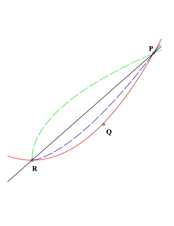
Figure 1. The graph of $h_{k}(t)=t^{k}$, $k=\frac{1}{2},1,\frac{3}{2}$ (green, black, blue), respectively, and $f(t)=t^{2}$ (red), $t\in[0,1]$.

Hence, 1.5 means geometrically that for a given three non-collinear points $P,Q$ and $R$ on the graph of $f$ with $Q$ between $P$ and $R$ (say $P<Q<R$). Let $h$ is super(sub)multiplicative and $h\left(\alpha\right)\geq(\leq)\,\alpha$, for $\alpha\in\left(0,1\right)\subset J$. A function $f$ is $h$–convex (concave) if $Q$ is on or below (above) the $h$-chord $\widehat{PR}$ (see Figure 1).

Caution: In special case, for $h_{k}\left(t\right)=t^{k}$, $t\in\left(0,1\right)$ the proposed geometric interpretation is valid for $k\in(-1,0)\cup(0,\infty)$. In the case that $k\leq-1$ or $k=0$ the geometric meaning is inconclusive so we exclude this case (and (and similar cases) from our proposal above.

Definition 11.

Let $h:J\to\left(0,\infty\right)$ be a non-negative function. Let $f:I\to\mathbb{R}$ be any function. We say $f$ is $h$-midconvex ($h$-midconcave) if

$$f\left({\frac{{x+y}}{2}}\right)\leq(\geq)\,h\left({\frac{1}{2}}\right)\left[{f\left(x\right)+f\left(y\right)}\right]$$

for all $x,y\in I$.

In particular, $f$ is locally $h$-midocnvex if and only if

$$h\left({\frac{1}{2}}\right)\left[f\left({x+p}\right)+f\left({x-p}\right)\right]-f\left(x\right)\geq 0,$$

for all $x\in\left(x-p,x+p\right)$, $p>0$.

A generalization of Jensen characterization of convex functions could be stated as follows:

Theorem 1.

Let $h:J\to\left(0,\infty\right)$ be a non-negative function such that $h\left(\alpha\right)\geq\alpha$, for all $\alpha\in(0,1)$. Let $f:I\to\mathbb{R}_{+}$ be a nonnegative continuous function. $f$ is $h$-convex if and only if it is $h$-midconvex; i.e., the inequality

$$f\left({\frac{{x+y}}{2}}\right)\leq h\left({\frac{1}{2}}\right)\left[{f\left(x\right)+f\left(y\right)}\right],$$

holds for all $x,y\in I$.

Proof.

The first direction follows directly by definition of $h$-convexity. To prove the second direction, suppose on the contrary that $f$ is not $h$-convex. Then, there exists a subinterval $[x,y]$ such that the graph of $f$ is not under the chord joining $(x,f(x))$ and $(y,f(y))$; that is,

$$f\left(t\right)\geq\left[{f\left(y\right)-f\left(x\right)}\right]h\left(\frac{t-x}{y-x}\right)+f\left(x\right)=L(t;h),$$

for all such $x,y\in I\cap J$. In other words, the function

$$g\left(t\right)=f\left(t\right)-\left[{f\left(y\right)-f\left(x\right)}\right]h\left({\frac{{t-x}}{{y-x}}}\right)-f\left(x\right),\qquad t\in I$$

satisfies $M=\sup\left\{{g\left(t\right):t\in[x,y]}\right\}>0$. Since $h\left(0\right)=0$ and $h\left(1\right)=1$, then $L\left(x;h\right)=f\left(x\right)$ and $L\left(y;h\right)=f\left(y\right)$, so that the $h$-cord $L$ agrees with $f$ at endpoints $x,y$. Thus, $g$ is continuous and $g(x)=g(y)=0$, direct computation shows that $g$ is also mid $h$-convex. Setting $c=\inf\left\{{t\in[x,y]:g\left(t\right)=M}\right\}$, then necessarily $g(c)=M$ and $c\in(x,y)$. By the definition of $c$, for every $p>0$ for which $c\pm p\in(a,b)$, we have $g\left({c-p}\right)<g\left(c\right)$ and $g\left({c+p}\right)<g\left(c\right)$, so that since $h\left(\alpha\right)\geq\alpha$, for all $\alpha\in(0,1)$ we have

$$g\left({c-p}\right)+g\left({c+p}\right)<2g\left({c}\right)=\frac{1}{\frac{1}{2}}g\left({c}\right)\leq\frac{1}{h\left({\frac{1}{2}}\right)}g\left({c}\right)$$

which contradicts the fact that $g$ is mid $h$-convex. ∎

Corollary 1.

Let $h:J\to\left(0,\infty\right)$ be a non-negative function such that $h\left(\alpha\right)\leq\alpha$, for all $\alpha\in(0,1)$. Let $f:I\to\mathbb{R}_{+}$ be a nonnegative continuous function. $f$ is $h$-concave if and only if it is $h$-midconcave.

Sometimes we often need to know how fast limits are converging, and this allows us to control the remainder of a given function in a neighborhood of some point $x_{0}$. So that, we need to extend the concept of continuity. Fortunately, in control theory and numerical analysis, a function $h:J\subseteq[0,\infty)\to[0,\infty]$ is called a control function if

1. $h$ is nondecreasing,

2. $\inf_{\delta>0}h\left(\delta\right)=0$.

A function $f:I\to\mathbb{R}$ is $h$-continuous at $x_{0}$ if $\left|f\left(x\right)-f\left(x_{0}\right)\right|\leq h\left(|x-x_{0}|\right)$, for all $x\in I$. Furthermore, a function is continuous in $x_{0}$ if it is $h$-continuous for some control function $h$.

This approach leads us to refining the notion of continuity by restricting the set of admissible control functions.

For a given set of control functions $\mathcal{C}$ a function is $\mathcal{C}$-continuous if it is $h$-continuous for all $h\in\mathcal{C}$. For example the Hölder continuous functions of order $\alpha\in(0,1]$ are defined by the set of control functions

$$\mathcal{C}^{(\alpha)}_{H}\left(h\right)=\left\{h|h\left(\delta\right)=H\left|\delta\right|^{\alpha},H>0\right\}$$

In case $\alpha=1$, the set $\mathcal{C}^{(1)}_{H}\left(h\right)$ contains all functions satisfying the Lipschitz condition.

Theorem 2.

Let $(0,1)\subseteq J$, $h:J\to\left(0,\infty\right)$ be a control function which is supermultiplicative such that $h(\alpha)\geq\alpha$ for each $\alpha\in(0,1)$. Let $I$ be a real interval, $a,b\in\mathbb{R}$ $(a<b)$ with $a,b$ in $I^{\circ}$ (the interior of $I$). If $f:I\to\mathbb{R}$ is non-negative $h$-convex function on $[a,b]$, then $f$ is $h$-continuous on $[a,b]$.

Proof.

Choose $\epsilon>0$ be small enough such that $\left(a-\epsilon,b+\epsilon\right)\subseteq I$ and let

$$m_{\epsilon}:=\inf\left\{{f\left(x\right),x\in\left({a-\epsilon,b+\epsilon}\right)}\right\}\qquad\text{and}\qquad M_{\epsilon}:=\sup\left\{{f\left(x\right),x\in\left({a-\epsilon,b+\epsilon}\right)}\right\},$$

such that $h\left(\epsilon\right)=M_{\epsilon}-m_{\epsilon}$. If $x,y\in\left[a,b\right]$, such that $x=y+\frac{\epsilon}{\left|y-x\right|}\left(y-x\right)$ and $\lambda_{\epsilon}=\frac{\left|y-x\right|}{\epsilon+\left|y-x\right|}$. Then for $z\in\left[a-\epsilon,b+\epsilon\right]$, $y=\lambda_{\epsilon}z+\left(1-\lambda_{\epsilon}\right)x$, we have

$$f\left(y\right)=f\left({\lambda_{\epsilon}z+\left({1-\lambda_{\epsilon}}\right)x}\right) \leq\lambda_{\epsilon}f\left(z\right)+\left({1-\lambda_{\epsilon}}\right)f\left(x\right)$$

$$\leq\lambda_{\epsilon}\left[{f\left(z\right)-f\left(x\right)}\right]+f\left(x\right)\leq h\left(\lambda_{\epsilon}\right)\left[{f\left(z\right)-f\left(x\right)}\right]+f\left(x\right),$$

which implies that $y=\lambda_{\epsilon}z+\left(1-\lambda_{\epsilon}\right)x$, we have

$$f\left(y\right)-f\left(x\right)\leq h\left(\lambda_{\epsilon}\right)\left[{f\left(z\right)-f\left(x\right)}\right] \leq h\left(\lambda_{\epsilon}\right)\left({M_{\epsilon}-m_{\epsilon}}\right)$$

$$<h\left({\frac{{\left|{y-x}\right|}}{\epsilon}}\right)\left({M_{\epsilon}-m_{\epsilon}}\right)$$

$$<\frac{{h\left({\left|{y-x}\right|}\right)}}{{h\left(\epsilon\right)}}\left({M_{\epsilon}-m_{\epsilon}}\right)$$

$$=h\left({\left|{y-x}\right|}\right).$$

Since this is true for any $x,y\in\left[a,b\right]$, we conclude that $\left|f\left(y\right)-f\left(x\right)\right|\leq h\left({\left|{y-x}\right|}\right)$, which shows that $f$ is $h$-continuous on $\left[a,b\right]$ as desired. ∎

Another Proof. Alternatively, if one replaces the condition $h(\alpha)+h(1-\alpha)\leq 1$ for each $\alpha\in(0,1)$ instead of $h(\alpha)\geq\alpha$ in Theorem 2. Then by repeating the same steps in the above proof, we have

$$f\left(y\right)=f\left({\lambda_{\epsilon}z+\left({1-\lambda_{\epsilon}}\right)x}\right) \leq h\left(\lambda_{\epsilon}\right)f\left(z\right)+h\left({1-\lambda_{\epsilon}}\right)f\left(x\right)$$

$$\leq h\left(\lambda_{\epsilon}\right)f\left(z\right)+\left[{1-h\left(\lambda_{\epsilon}\right)}\right]f\left(x\right)\qquad({\rm{since}}\,\,\,h\left({1-\lambda_{\epsilon}}\right)\leq 1-h\left(\lambda_{\epsilon}\right))$$

$$=h\left(\lambda_{\epsilon}\right)\left[{f\left(z\right)-f\left(x\right)}\right]+f\left(x\right),$$

which implies that $y=\lambda_{\epsilon}z+\left(1-\lambda_{\epsilon}\right)x$, we have

$$f\left(y\right)-f\left(x\right)\leq h\left(\lambda_{\epsilon}\right)\left[{f\left(z\right)-f\left(x\right)}\right] \leq h\left(\lambda_{\epsilon}\right)\left({M_{\epsilon}-m_{\epsilon}}\right)$$

$$<h\left({\frac{{\left|{y-x}\right|}}{\epsilon}}\right)\left({M_{\epsilon}-m_{\epsilon}}\right)$$

$$<\frac{{h\left({\left|{y-x}\right|}\right)}}{{h\left(\epsilon\right)}}\left({M_{\epsilon}-m_{\epsilon}}\right)$$

$$=h\left({\left|{y-x}\right|}\right).$$

Since this is true for any $x,y\in\left[a,b\right]$, we conclude that $\left|f\left(y\right)-f\left(x\right)\right|\leq h\left({\left|{y-x}\right|}\right)$, which shows that $f$ is $h$-continuous on $\left[a,b\right]$. Surely, this is can be considered as an alternative proof of Theorem 2.

It’s well known that if $f$ is twice differentiable then $f$ is convex if and only if $f^{\prime\prime}\geq 0$. In a convenient way Pinheiro in [29] proposed that $f$ is an $s$-convex (in the second sense) if and only if $f^{\prime\prime}\geq 1-2^{1-s}$. Indeed, Pinheiro presented a “proof” to her result, however we can say without doubt that she introduced some good thoughts rather than formal mathematical proof. Following the same way in [29] and in viewing the presented discussion in the introduction we conjecture that:

Conjecture 1.

Let $h:J\to\left(0,\infty\right)$ be a non-negative function such that $h\left(\alpha\right)\geq\alpha$, for all $\alpha\in(0,1)$, and consider $f:I\to\mathbb{R}$ be a twice differentiable function. A function $f$ is $h$-convex if and only if $f^{\prime\prime}\left(x\right)\geq 1-2h\left(\frac{1}{2}\right)$.

References

- [1] M.W. Alomari, M. Darus, S.S. Dragomir and U. Kirmaci, On fractional differentiable -convex functions, Jordan J. Math and Stat., (JJMS), 3 (1) (2010), 33–42.
- [2] M. Bombardelli and S. Varošanec, Properties of -convex functions related to the Hermite-Hadamard-Fejér inequalities, Compute. Math. Applica., 58 (9) (2009), 1869–1877.
- [3] W.W. Breckner, Stetigkeitsaussagen für eine Klasse verallgemeinerter konvexer funktionen in topologischen linearen Räumen, Publ. Inst. Math., 23 (1978), 13–20.
- [4] W. W. Breckner and G. Orban, Continuity properties of rationally s-convex mappings with values in an ordered topological linear space, Babes-Bolyai University, Cluj-Napocoi (1978).
- [5] W.W. Breckner, Hölder-continuity of certain generalized convex functions, Optimization, 28 (1994), 201–209.
- [6] W. W. Breckner, Rational -convexity, a generalized Jensen-convexity. Cluj-Napoca: Cluj University Press, 2011.
- [7] S. Cobzas, and I. Muntean, Continuous and locally Lipschitz convex functions, Mathematica Rev. d’Anal. Numér. et de Théorie de I’Approx., Ser. Mathematica, 18 (41) (1976), 41–51.
- [8] S. Cobzas, On the Lipschitz properties of continuous convex functions, Mathematlca Ret. d’Anal. Numér. et de Théorie de I’Approx., Ser. Marhemarica, 21 (44) 1979, 123?125.
- [9] M.V. Cortez, Relative strongly -convex functions and integral inequalities, Appl. Math. Inf. Sci. Lett., 4 (2) (2016), 39–45.
- [10] S.S. Dragomir, Inequalities of Jensen type for -convex functions on linear spaces, Math. Moravica, 19 (1) (2015), 107–121.
- [11] S.S. Dragomir, Inequalities of Hermite-Hadamard type for -convex functions on linear spaces, Proyecciones J. Math., 34 (4) (2015), 323–341.
- [12] S.S. Dragomir, J. Pečarić and L.E. Persson, Some inequalities of Hadamard type, Soochow J. Math., 21 (1995) 335–341.
- [13] E.K. Godunova and V.I. Levin, Neravenstva dlja funkcii širokogo klassa, soderžaščego vypuklye, monotonnye i nekotorye drugie vidy funkcii, Vyčislitel. Mat. i. Mat. Fiz. Me?vuzov. Sb. Nau?c. Trudov, MGPI, Moskva, 1985, 138–142.
- [14] A. Házy, Bernstein-doetsch type results for -convex functions, Math. Inequal. Appl., 14 (3) (2011), 499–508.
- [15] H. Hudzik and L. Maligranda, Some remarks on -convex functions, Aequationes Math., 48 (1994), 100–111.
- [16] M. Matłoka, On Hadamard’s inequality for -convex function on a disk, Appl. Math. Comp.,235 (2014), 118–123.
- [17] J. Musielak, Orlicz spaces and Modular spaces, Lecture Notes in Mathematics, Springer-Verlag, Berlin Heidelberg, 1983.
- [18] W. Matuszewska and W. Orlicz, A note on the theory of -normed spaces of -integrable functions, Studia Math., 21, 1981 , 107–115.
- [19] D.S. Mitrinović and J. Pečarić, Note on a class of functions of Godunova and Levin, C. R. Math. Rep. Acad. Sci. Can., 12 (1990), 33–36.
- [20] D.S. Mitrinović, J. Pečarić and A.M. Fink, Classical and New Inequalities in Analysis, Kluwer Academic, Dordrecht, 1993.
- [21] C.P. Niculescu, L.E. Persson, Convex Functions and Their Applications. A Contemporary Approach, CMS Books Math., vol. 23, Springer-Verlag, New York, 2006.
- [22] A. Olbryś, Representation theorems for -convexity, J. Math. Anal. Appl, 426 (2)(2015), 986–994.
- [23] C.E.M. Pearce and A.M. Rubinov, -functions, quasi-convex functions and Hadamard-type inequalities, J. Math. Anal. Appl., 240 (1999), 92–104.
- [24] M. Pycia, A direct proof of the -Hölder continuity of Breckner -convex functions, Aequationes Math., 61 (1-2), (2001), 128–130.
- [25] M.R. Pinheiro, Convexity Secrets, Trafford Publishing, 2008.
- [26] M.R. Pinheiro, Exploring the concept of -convexity, Aequationes Mathematicae, 74 (3) (2007), 201–209.
- [27] M.R. Pinheiro, Hudzik and Maligranda’s -convexity as a local approximation to convex functions, Preprint, 2008.
- [28] M.R. Pinheiro, Hudzik and Maligranda’s -convexity as a local approximation to convex functions II, Preprint, 2008.
- [29] M.R. Pinheiro, Hudzik and Maligranda’s -convexity as a local approximation to convex functions III, Preprint, 2008.
- [30] M.R. Pinheiro. H–H Inequality for -Convex Functions, Inter. J. P. Appl. Math., 44 (4) (2008), 563–579.
- [31] A. W. Roberts and D. E. Varberg, Convex Functions, Academic Press, New York, 1973.
- [32] S. Rolewicz, Metric Linear Spaces, 2nd ed., PWN, Warsaw, 1984.
- [33] T. Trif, Hölder continuity of generalized convex set-valued mappings, J. Math. Anal. Appl., 255 (2001), 44–57.
- [34] K.-L. Tseng, G.-S. Yang and S.S. Dragomir, On quasi convex functions and Hadamard’s inequality, Demonsrtatio Mathematics, XLI (2) (2008), 323–335.
- [35] S. Varošanec, On -convexity, J. Math. Anal. Appl., 326 (2007), 303–311.