FFT and orthogonal discrete transform on weight lattices of semi-simple Lie groups

Abstract

We give two algebro-geometric inspired approaches to fast algorithms for Fourier transforms in algebraic signal processing theory based on polynomial algebras in several variables. One is based on module induction and one is based on a decomposition property of certain polynomials. The Gauss-Jacobi procedure for the derivation of orthogonal transforms is extended to the multivariate setting. This extension relies on a multivariate Christoffel-Darboux formula for orthogonal polynomials in several variables. As a set of application examples a general scheme for the derivation of fast transforms of weight lattices based on multivariate Chebyshev polynomials is derived. A special case of such transforms is considered, where one can apply the Gauss-Jacobi procedure.

1 Introduction

The popularization of the fast Fourier transform (FFT) algorithm by Cooley and Tukey Cooley.Tukey:1965 paved the way to productive applications of the discrete Fourier transform. Due to its numerous applications the fast Fourier transform has been termed to be one of the most important algorithms of the twentieth century. The usage of algebra in the theory of fast Fourier transform algorithms dates back at least until the work of Nicholson Nicholson:1971a . Algebraic approaches to FFT algorithms split into two main directions: group algebra and polynomial algebra approaches. The interpretation of the fast Fourier transform in terms of the cyclic group $Z_{n}$ was introduced in Nicholson:1971a . This group-based approach allows for a generalization of FFT algorithms to non-abelian groups as in Diaconis.Rockmore:1990a . The polynomial algebra approach relies on the insight that there exists an isomorphism of algebras $\mathbb{C}[Z_{n}]\cong\mathbb{C}[x]\big{/}\langle\;x^{n}-1{\;}\rangle$. This approach allows to study another large class of FFT algorithms Beth:1984a ; Heideman.Burrus:1986a ; Johnson.Burrus:1985a relying on ideas of Nussbaumer Nussbaumer:1982a and Winograd Winograd:1979a . The full polynomial algebra approach was worked out in Pueschel.Moura:2006 ; Pueschel.Moura:2008a ; Pueschel.Moura:2008b ; Pueschel.Moura:2008c leading to algebraic signal processing theory. This theory captures not only the derivation of fast algorithms for different signal models but treats the most important concepts from linear signal processing, e.g. $z$-transform, signals, filters, and Fourier transform, algebraically, as well. One main difference in algebraic signal processing when compared to other recent approaches, like the decomposition of semi-simple algebras using Bratelli-diagramms in Maslen.Rockmore.Wolff:2017a , is that in algebraic signal processing one decomposes modules. This is motivated by the fact that in algebraic signal processing theory the signals are modeled as a module over the algebra of filters. This approach immediately leads to explicit matrix factorizations.

In algebraic signal processing theory one can identify three approaches for the derivation of fast algorithms for Fourier transforms of algebraic signal models based on polynomials. Even though all three approaches are essentially based on the Chinese remainder theorem and a stepwise partial decomposition, the different details lead to algorithms of different complexity.

The first one is based on a factorization of polynomials $f(x)=g(x)\cdot h(x)$. This approach requires no special conditions on the polynomial $f$ but leads to sub-optimal $O(n\log^{2}n)$ algorithms.

The second approach is based on the decomposition property $f(x)=p(q(x))$ of certain polynomials. This approach gives optimal $O(n\log n)$ algorithms. Unfortunately in one variable the only families of polynomials posessing this property are, up to affine-linear coordinate changes, the monomials $x^{n}$ and the Chebyshev polynomials $T_{n}(x)$ Rivlin:1974a . Hence the only $O(n\log n)$ algorithms for signal models based on polynomials in one variable derivable by this method are the Cooley-Tukey-type algorithms for the trigonometric, i.e. sine and cosine transforms associated to Chebyshev polynomials, and the discrete Fourier transform, associated to the monomials. In several variables it is not known Vesolov:1991a if there are, up to affine-linear coordinate changes, any examples of polynomials with this property except the monomials and multivariate Chebyshev polynomials. The second approach in combination with multivariate Chebyshev polynomials was used to derive fast algorithms for undirected hexagonal Pueschel.Roetteler:2008 and FCC lattices Seifert.Hueper.Uhl:2018a .

As there are other algorithms for the discrete Fourier transform, like the Britanak-Rao-FFT Britanak.Rao:1999a , one might wonder if these algorithms can be derived using algebraic signal processing theory. This question was solved using the third approach. Here one relies on induced modules. This approach raises the level of abstraction by not relying on properties of the polynomials but on properties of the signal modules. Module induction is based on an algebra $\mathscr{A}$ with subalgebra $\mathscr{B}$ and a finite set $T\subset\mathscr{A}$, the transversal, such that $\mathscr{A}=\bigoplus_{t\in T}t\mathscr{B}$. The induced $\mathscr{A}$-module $N$ of a $\mathscr{B}$-module $M$ is $N=\bigoplus_{t\in T}t\mathbin{\triangleright}M$, where $\mathbin{\triangleright}$ denotes the action of the algebra on the module. In Sandryhaila.Kovacevic.Pueschel:2011 this approach was worked out for polynomial algebras in one variable with regular modules. As applications general-radix algorithms for the Britanak-Rao Britanak.Rao:1999a and the Wang-FFT Wang:1984a were deduced.

The first part of this article extends the third and second approach to polynomial algebras in several variables. For this a very general decomposition of modules is used to derive a decomposition of the Fourier marices. This is necessary since unlike in the univariate case for multivariate polynomials the decomposition property in general does not yield an induction. We given an interpretation of the underlying mechanisms in the language of algebraic geometry, as well. This is useful since it clarifies many aspects of the theory. As an application example it is shown how one can derive the FFT for a directed hexagonal lattice in this setting. By deriving this fast algorithm for the directed hexagonal lattice it is illustrated how to rederive the fast algorithms of Mersereau and Speake Mersereau.Speake:1981a for regular directed lattices within algebraic signal processing theory.

The connection of orthogonal polynomial transforms and univariate orthogonal polynomials is well-known Yemini.Pearl:1979a . Using the Christoffel-Darboux formula the Gauß-Jacobi-procedurce of Yemini.Pearl:1979a allows to derive an orthogonal version of any discrete polynomial transform based on orthogonal polynomials. Even though there is a rather mature theory of orthogonal polynomials in several variables Xu:2017a the connection to signal processing is not vivid in the literature. Only recently the author used the multivariate Christoffel-Darboux formula of Xu Xu:1993a to derive an orthogonal version of a discrete cosine transform on lattices of triangles Seifert.Hueper:2018b . Unfortunately this method does not work in every case but relies on the same condition as the existence of a Gaussian cubature formula as zeros of the orthogonal polynomials. This is deplorable since Gaussian cubatures rarely exist Li.Xu:2010 . In the second part we derive the general orthogonalization scheme and show that the existence of such a Gaussian cubature implies the existence of an orthogonal discrete transform for the signal model corresponding to the polynomials used to construct the cubature.

Fast transforms for regular undirected lattices have been derived for the hexagonal lattice Pueschel.Roetteler:2008 and for the FCC lattice Seifert.Hueper.Uhl:2018a . Both algorithms are special cases of a whole family, based on generalization of the Chebyshev polynomials to multivariate polynomials intimately connected to Lie theory. One of the first attempts to study these polynomials in two variables was Koornwinder:1974 . The multivariate version was first defined in Lidl:1975 . Important properties were deduced in Eier.Lidl:1982 . The semigroup property was first proven in Ricci:1986 . None of these approaches realised the connection to Lie groups, which was clarified in Hoffman.Withers:1988a . Although Chebyshev polynomials in one variable are ubiquitous in applied mathematics, their multivariate counterparts only recently started to penetrate into applications. Meanwhile, there are applications to the discretization of partial differential equations Munthe-Kaas:2006 ; Ryland.Munthe-Kaas:2011 ; Munthe-Kaas.Nome.Ryland:2012 , cubature formulas Li.Xu:2010 ; Moody.Patera:2011 ; Hrivnak.Motlochova.Patera:2016 and discrete transforms Atoyan.Patera:2007 ; Hrivnak.Motlochova:2014 ; Hrivnak.Motlochova:2018a . From an algebraic signal processing perspective they are interesting for two reasons. First they are examples of multivariate polynomials with the decomposition property. Thus the multivariate Chebyshev polynomials yield application examples of the generalized second approach to fast Fourier transforms. Second they are intimately connected to weight lattices of semi-simple Lie groups. As some of the weight lattices are associated to densest sphere packings (Conway.Sloane:1999, , Ch. 4), the multivariate Chebyshev polynomials give in these cases rise to fast transforms of optimally sampled signals Petersen.Middleton:1962 ; Kuensch.Agrell.Hamprecht:2005 .

We derive fast algorithms in the cases of Chebyshev polynomials associated to Lie algebras of type $A_{2}$ and $C_{2}$. Furthermore we show that in the case $C_{2}$ the multivariate Gauss-Jacobi procedure is applicable.

The main contributions of this paper are as follows. In Sect. 2 the induction-based approach Sandryhaila.Kovacevic.Pueschel:2011 and the approach relying on the decomposition property Pueschel.Roetteler:2008 for the derivation fast algorithms in algebraic signal processing theory are extended to a more general situation and polynomials in several variables. Furthermore it is shown that in the multivariate case the decomposition property yields another decomposition theorem for Fourier transforms. In Sect. 3 a generalization of the Gauß-Jacobi-procedure for the derivation of orthogonal transforms is derived. Finally in Sect. 4 we state a general scheme for the derivation of fast transform algorithms for undirected weight lattices of semi-simple Lie algebras based on multivariate Chebyshev polynomials.

2 An algebro-geometric perspective on signal processing and FFT

Algebraic signal processing theory enlightens the algebraic structures underlying linear signal processing technqiues Pueschel.Moura:2006 ; Pueschel.Moura:2008a ; Pueschel.Moura:2008b . From a signal processing perspective the algebraic structures can be motivated as follows. If one considers the basic operations on filters, i.e. putting them in series and parallel and amplifying them, one can interpret these operations as addition, multiplication and scalar multiplication, respectively. One observes that these operations are subject to a distributive law. Consequently the filters can mathematically be described by an algebra with respect to these operations. Furthermore, one can add and amplify signals, and we can apply filters to signals. From a mathematical point of view one thus gets the structure of a module over the algebra of filters for the signals, with application of filters to signals as algebra action. The $z$-transform is a bijective mapping from a set of numbers, the samples, to signals, which embody more structure. In this way, the $z$-transform tells how to translate samples to signals.

An algebraic signal model, a triple $(\mathscr{A},M,\Phi)$ consisting of a $\mathbb{C}$-algebra $\mathscr{A}$, a free $\mathscr{A}$-module $M$, and a bijective mapping $\Phi\colon\mathbb{C}^{n}\to M$ for some $n\in\mathbb{N}\cup\{\infty\}$. By the previous considerations this is motivated as the main object to study in algebraic signal processing theory.

We recall the first example of algebraic signal processing theory, the classical finite time discrete signal processing. In the classical theory one considers a set of numbers $s=(s_{0},\dots,s_{n-1})\in\mathbb{C}^{n}$ as signal and extends it periodically, i.e. $s_{N}=s_{N\mkern 4.0mu{\operator@font mod}\mkern 6.0mun}$ for any $N\in\mathbb{Z}$. A set of samples $s\in\mathbb{C}^{n}$ is mapped to a polynomial in $x=z^{-1}$ by the $z$-transform

$$\Phi_{d}\colon(s_{0},\dots,s_{n-1})\mapsto\sum_{i=0}^{n-1}s_{i}x^{i}.$$ (1)

To capture the periodic extension of the signal, one considers the resulting polynomials modulo $x^{n}-1$ or, more precisely, modulo the ideal generated by $x^{n}-1$. This results in an element of the set $\mathbb{C}[x]\big{/}\langle\;x^{n}-1{\;}\rangle$. The filters in classical signal processing are generated by a shift. A shift is realized on the polynomials as multiplication by $x$

$$x\cdot\Phi(s)=x\sum_{i=0}^{n-1}s_{i}x^{i}=\sum_{i=0}^{n-1}s_{i-1\mkern 4.0mu{\operator@font mod}\mkern 6.0mun}x^{i}.$$ (2)

This results in a delay of the signal. The filters are the polynomials in the shift $x$, i.e. elements of $\mathbb{C}[x]\big{/}\langle\;x^{n}-1{\;}\rangle$. The structural difference between signal and filters is the algebraic structure. The set of filters is equipped with the structure of an algebra, while the signals form a module over the algebra of filters. In this example we thus get the following structures. Let $h_{1},h_{2}\in\mathbb{C}[x]\big{/}\langle\;x^{n}-1{\;}\rangle$ be two filters and $c\in\mathbb{C}$, then $h_{1}(x)\cdot h_{2}(x)$, $h_{1}(x)+h_{2}(x)$ and $c\cdot h_{i}(x)$ form new filters. For two signals $s_{1},s_{2}\in\mathbb{C}[x]\big{/}\langle\;x^{n}-1{\;}\rangle$ only $s_{1}(x)+s_{2}(x)$ and $c\cdot s_{1}(x)$ form new signals, i.e. one has the structure of a vector space. But additionally $h_{i}(x)\cdot s_{i}(x)$ forms a new filter, as well, which turns the signals into a module over the algebra of filters. Hence the finite time discrete signal processing translates to the model $(\mathscr{A}_{d},M_{d},\Phi_{d})$, with underlying sets $\mathscr{A}_{d}=M_{d}=\mathbb{C}[x]\big{/}\langle\;x^{n}-1{\;}\rangle$, in algebraic signal processing theory.

A signal model can be visualized by a graph. The visualization is given by the following construction. First one associates to each basis element of the module a node. An edge from one node to another is added if the result of the action of a generator of the algebra, i.e. a shift, on the basis element associated to the first node contains non-zero coefficient to the basis element of the second node. The visualization of the discrete finite time model is shown in Fig. 1.

Figure 1: Visualization of the finite, discrete time signal model.

Since the boundary conditions of two- or three-dimensional models tend to lead to confusing pictures, the boundary connections are often omitted. Note that these visualization graphs motivated a path to signal processing on graphs see e.g. Sandryhaila.Moura:2013a .

An algebraic signal model gives rise to a notion of Fourier transform based on the decomposition of the signal module. Assume $M\cong\bigoplus_{i}M_{i}$ can be decomposed into irreducible modules. Any isomorphism

$$\mathcal{F}\colon M\to\bigoplus_{i}M_{i}$$ (3)

is called a Fourier transform for the associated algebraic signal model. For the finite time discrete signal processing model one has the decomposition

$$\mathbb{C}[x]\big{/}\langle\;x^{N}-1{\;}\rangle\cong\bigoplus_{j=0}^{N-1}\mathbb{C}[x]\big{/}\langle\;x-\mathrm{e}^{2\pi\mathrm{i}j/N}{\;}\rangle.$$ (4)

Choosing as basis $[1,x,\dots,x^{N-1}]$ in $\mathbb{C}[x]\big{/}\langle\;x^{N}-1{\;}\rangle$ and $[1]$ in each $\mathbb{C}[x]\big{/}\langle\;x-\mathrm{e}^{2\pi\mathrm{i}j/N}{\;}\rangle$ the isomorphism (4) can be realized by the $N\times N$-matrix

$$\left[\mathrm{e}^{2\pi\mathrm{i}j\cdot k/N}\right]_{j,k},$$ (5)

which is the discrete Fourier transform matrix.

Fast algorithms for these Fourier transforms rely on step-wise application of the Chinese remainder theorem. We recall the basic notations needed, for a more detailed treamtent see e.g. (Lang:2002a, , Ch. II). Recall that ideals $I_{1},I_{2}$ of a ring $R$ are called coprime if $I_{1}+I_{2}=R$. Typical examples of coprime ideals in the polynomial algebra $\mathbb{C}[x]$ are the ideals $\langle\;x-a{\;}\rangle$ and $\langle\;x-b{\;}\rangle$ with scalars $a\not=b$. For any commutative ring $R$ with ideal $I=I_{1}\cap\dots\cap I_{n}$, such that all $I_{i}$ are coprime, one has an isomorphism

$$R\big{/}I\longrightarrow R\big{/}I_{1}\times\dots\times R\big{/}I_{n}.$$ (6)

Tensoring this isomorphism with an $R$-module $M$ yields the Chinese remainder theorem for modules

$$M\big{/}IM\longrightarrow M\big{/}I_{1}M\times\dots\times M\big{/}I_{n}M.$$ (7)

We are especially interested in algebras of polynomials in several variables. This is motivated by two considerations. First, group algebras and algebras of polynomials in one variable have been investigated already thoroughly. Second, algebras of polynomials in several variables are intimately connected to algebraic geometry. This allows one to get a geometric point of view for signal processing concepts. One immediate obstacle using polynomials in multiple variables is that their zero-sets are in general non-discrete. Hence one has to be aware that we will consider only very special cases of polynomial algebras.

For the geometric point of view recall the Hilbert Nullstellensatz (Lang:2002a, , Ch. IX), which states that there is a correspondence between ideals of a polynomial algebra and varieties. A variety is a subset of $\mathbb{C}^{n}$, being the set of common zeros of all polynomials in the ideal. This correspondence is not one-to-one since for example $\langle\;x{\;}\rangle$ and $\langle\;x^{2}{\;}\rangle$ have the same variety $\mathsf{V}(\langle\;x{\;}\rangle)=\mathsf{V}(\langle\;x^{2}{\;}\rangle)=\{0\}$. But the correspondence becomes one-to-one if one restricts to radical ideals. An ideal $I$ of an algebra $\mathscr{A}$ is called radical if $I=\sqrt{I}=\{a^{n}\;|\;a\in I,n\in\mathbb{N}\}$. For example the radical ideal of $\langle\;x^{2}{\;}\rangle$ is $\langle\;x{\;}\rangle$. Radicality of an ideal is the several variables analog of square-freeness of polynomials in one variable. An ideal is called zero-dimensional if its variety $\mathsf{V}(I)$ is finite. In this paper we assume all ideals to be radical and zero-dimensional. If this is not the case for some example, we will explicitly state that and use the radical ideal.

Another problem with multivariate polynomials is that in general division by the generators of an ideal is not well-defined. That is one can get different results of the division by changing the sequence of which generator to divide by. The crucial notion to avoid this problem is that of a Gröbner basis. A Gröbner basis is a special set of generators of an ideal depending on the choice a monomial order, see Cox.Little.OShea:2015 for details. By the Buchberger criterion a set of polynomials forms a Gröbner basis if their leading monomials with respect to the choosen monomial order are disjoint. In this paper we rely on this criterion only to decide whether a given set of generators is a Gröbner basis.

Additionally to the algebra $\mathscr{A}$ we are considering an $\mathscr{A}$-module. The geometric counterpart of a module over an algebra is a vector bundle over a space. This is formalized by the Serre-Swan theorem, see e.g. Morye:2013a . The Serre-Swan theorem states that the sections of vector bundles are precisely the projective, finitely generated modules over the algebra of functions of the underlying space. So the module of signals of an algebraic signal model can be interpreted as sections of vector bundles, cf. Fig. 2.

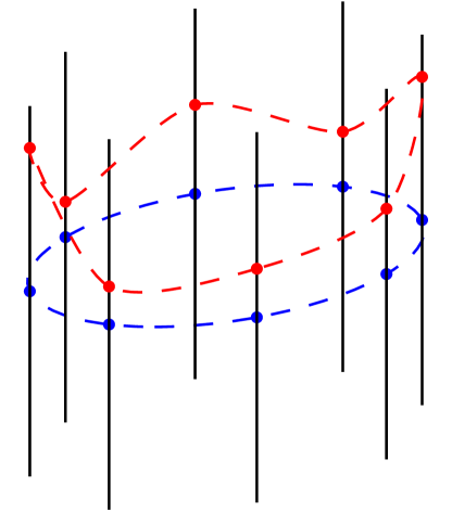
Figure 2: Sections of a vector bundle (red) over points on a circle (blue) form the signals of the finite, discrete time signal model.

Remark 1

In principle one does not need to restrain to $\mathbb{C}$ as the ground field. Indeed signal processing and Fourier transforms using finite fields might be of interest in some applications as these can be used for infinite precision calculations, see e.g. Lima.CampelloDeSouza:2011a . Nonetheless we will only consider algebras over $\mathbb{C}$ in this paper since this simplifies some arguments and definitions. If all the coefficients and varieties of appearing polynomials are real, we consider the structures over $\mathbb{R}$ without any loss.

We denote by $\Pi^{n}(x)=\mathbb{C}[x_{1},\dots,x_{n}]$ the space of all polynomials in $n$ indeterminates. Let the filter algebra be of the form $\mathscr{A}=\Pi^{n}(x)\big{/}I$ for some radical, zero-dimensional ideal $I$. Then by the Chinese remainder theorem we have

$$\Pi^{n}(x)\big{/}I\cong\bigoplus_{\alpha\in\mathsf{V}(I)}\Pi^{n}\big{/}\langle\;x_{1}-\alpha_{1},\dots,x_{n}-\alpha_{n}{\;}\rangle,$$ (8)

as all the $\langle\;x_{1}-\alpha_{1},\dots,x_{n}-\alpha_{n}{\;}\rangle$ are coprime as maximal ideals. The corresponding Fourier transform for the signal model with regular module is realized by the map

$$p(x_{1},\dots,x_{n})\mapsto\begin{bmatrix}p(\alpha)\end{bmatrix}_{\alpha\in\mathsf{V}(I)}.$$ (9)

If we choose a basis $B$ in the module $M=\Pi^{n}\big{/}I$ and the basis $[1]$ consisting of one only in each $\Pi^{n}\big{/}\langle\;x_{1}-\alpha_{1},\dots,x_{n}-\alpha_{n}{\;}\rangle$, the Fourier transform can be realized as multiplication with the matrix

$$P_{b,M}=[b(\alpha)]_{b\in B,\alpha\in\mathsf{V}(I)}.$$ (10)

If other bases than $[1]$ are used in each $\Pi^{n}(x)\big{/}\langle\;x_{1}-\alpha_{1},\dots,x_{n}-\alpha_{n}{\;}\rangle$, e.g. $[a_{i}]$ for $a_{i}\in\mathbb{C}$, the matrix changes to

$$P_{b,M}=\operatorname{\mathrm{diag}}\bigg{(}\frac{1}{a_{i}}\bigg{)}[b(\alpha)]_{b\in B,\alpha\in\mathsf{V}(I)}.$$ (11)

A fast algorithm for the Fourier transform $P_{b,M}$ is a factorization of the dense matrix $P_{b,M}$ into sparse matrices.

As motivation for the following we deduce the Cooley-Tukey FFT algorithm for the $\mathsf{DFT}$, first with a top-down Pueschel.Moura:2008c then with a bottom-up approach Sandryhaila.Kovacevic.Pueschel:2011 . This motivates the general theory. Consider the finite, discrete time signal model. If $n=m\cdot r$, we have $x^{n}=(x^{m})^{r}$, and $(x^{m})^{r}-1=\prod_{j=1}^{r}(x^{m}-\mathrm{e}^{2\pi\mathrm{i}j/r})$, as well as $x^{m}-\mathrm{e}^{2\pi\mathrm{i}j/r}=\prod_{k=1}^{m}(x-\mathrm{e}^{2\pi\mathrm{i}jk/(mr)})$. Hence we can decompose the module $\mathbb{C}[x]\big{/}\langle\;x^{n}-1{\;}\rangle$ in steps using the Chinese remainder theorem

$$\begin{split}\mathbb{C}[x]\big{/}\langle\;x^{n}-1{\;}\rangle&\longrightarrow\mathbb{C}[x]\big{/}\langle\;(x^{m})^{r}-1{\;}\rangle\\ &\longrightarrow\bigoplus_{j=1}^{r}\mathbb{C}[x]\big{/}\langle\;x^{m}-\mathrm{e}^{2\pi\mathrm{i}j/r}{\;}\rangle\\ &\longrightarrow\bigoplus_{j=}^{r}\bigoplus_{k=1}^{m}\mathbb{C}[x]\big{/}\langle\;x-\mathrm{e}^{2\pi\mathrm{i}jk/(rm)}{\;}\rangle\\ &\longrightarrow\bigoplus_{\ell=1}^{n}\mathbb{C}[x]\big{/}\langle\;x-\mathrm{e}^{2\pi\mathrm{i}\ell/n}{\;}\rangle.\end{split}$$ (12)

Each step is described by a sparse matrix and via the recursion step, we obtain the well-known $O(n\log(n))$ Cooley-Tukey algorithm in the case $n=2^{m}$. This is an example of the top-down approach for the derivation of FFT-like algorithms by algebraic signal processing theory used in Pueschel.Moura:2008c .

For a bottom-up approach we need to recall some tools from the representation theory of algebras. Consider a subalgebra $\mathscr{B}$ of the algebra $\mathscr{A}$. A finite set $T$ is called transversal if

$$\mathscr{A}=\bigoplus_{t\in T}t\mathscr{B}$$ (13)

as vector spaces. If $M$ is a $\mathscr{B}$-module, the module $\bigoplus_{t\in T}t\mathbin{\triangleright}M$, with vector space direct sum and $\mathbin{\triangleright}$ denoting the action of the algebra on the module, is the $T$-induced $\mathscr{A}$-module of $M$.

Now consider again the discrete finite time signal model with $n=m\cdot r$. Then the algebra $\mathscr{B}=\mathbb{C}[y]\big{/}\langle\;y^{m}-1{\;}\rangle$ is a subalgebra of $\mathscr{A}=\mathbb{C}[x]\big{/}\langle\;x^{n}-1{\;}\rangle$ generated by $y=x^{r}$. A transversal of $\mathscr{B}$ in $\mathscr{A}$ is given by $T=\{1,x,\cdots,x^{r-1}\}$. The identification of the regular module $\mathbb{C}[x]\big{/}\langle\;x^{n}-1{\;}\rangle$ with the induced module $\bigoplus_{t\in T}t\mathbb{C}[y]\big{/}\langle\;y^{m}-1{\;}\rangle$ is done by a basis change. This results in the decomposition

$$\begin{split}\mathbb{C}[x]\big{/}\langle\;x^{n}-1{\;}\rangle&\longrightarrow\bigoplus_{t\in T}t\mathbb{C}[y]\big{/}\langle\;y^{m}-1{\;}\rangle\\ &\longrightarrow\bigoplus_{t\in T}\bigoplus_{k=1}^{m}t\mathbb{C}[y]\big{/}\langle\;y-\mathrm{e}^{2\pi\mathrm{i}k/m}{\;}\rangle\\ &\longrightarrow\bigoplus_{\ell=1}^{n}\mathbb{C}[x]\big{/}\langle\;x-\mathrm{e}^{2\pi\mathrm{i}\ell/n}{\;}\rangle.\end{split}$$ (14)

Even though this decomposition resembles at a first glance the top-down approach, the explicit matrix form shows that these approaches are somewhat dual to each other. The top-down approach results in a decimation-in-frequency approach while the bottom-up yields a decimation-in-time approach. For example with $n=4=2\cdot 2$ the decomposition (12) leads to

$$\begin{bmatrix}1&1&1&1\\ 1&-\mathrm{i}&-1&\mathrm{i}\\ 1&-1&1&-1\\ 1&\mathrm{i}&-1&-\mathrm{i}\end{bmatrix}\\ =\begin{bmatrix}1&0&0&0\\ 0&0&0&1\\ 0&1&0&0\\ 0&0&1&0\end{bmatrix}\begin{bmatrix}1&1\\ 1&-1\\ &&1&\mathrm{i}\\ &&1&-\mathrm{i}\end{bmatrix}\begin{bmatrix}1&0&1&0\\ 0&1&0&1\\ 1&0&-1&0\\ 0&1&0&-1\end{bmatrix},$$ (15)

while the decomposition (14) gives

$$\begin{bmatrix}1&1&1&1\\ 1&-\mathrm{i}&-1&\mathrm{i}\\ 1&-1&1&-1\\ 1&\mathrm{i}&-1&-\mathrm{i}\end{bmatrix}\\ =\begin{bmatrix}1&0&1&0\\ 0&1&0&-\mathrm{i}\\ 1&0&-1&0\\ 0&1&0&\mathrm{i}\end{bmatrix}\begin{bmatrix}1&1\\ 1&-1\\ &&1&1\\ &&1&-1\end{bmatrix}\begin{bmatrix}1&0&0&0\\ 0&0&1&0\\ 0&1&0&0\\ 0&0&0&1\end{bmatrix}.$$ (16)

Hence both approaches lead to a sparse factorization of the matrices. Indeed in this case, as well as in general for univariate polynomials, both approaches can be described using induced modules. This relies on each of the modules $\mathbb{C}[x]\big{/}\langle\;x^{m}-\mathrm{e}^{2\pi\mathrm{i}j/r}{\;}\rangle$ being isomorphic. If one has more than one variable this is not true anymore. Furthermore, it might be advantageous to include more general modules and module actions than the regular module.

The basic idea for fast algorithms is stated in the following commutative diagram (17). It shows how one can decompose the $\mathscr{A}$-module $N$ stepwise if one can represent it a as an induction.

(17)

The diagram is cast into a theorem.

Theorem 2.1 (FFT algorithms, bottom-up approach)

Let $\mathscr{A}$ be an algebra with subalgebra $B$. Let $M_{t}=\Pi^{d}(y)\big{/}J_{t}$ be a set of $\mathscr{B}$-modules such that $N=\bigoplus_{t\in T}t\mathbin{\triangleright}M_{t}=\Pi^{n}\big{/}I$, with $T=\{t_{1},\dots,t_{w}\}\subset\mathscr{A}$ a finite set, is an $\mathscr{A}$-module. Assume the action of $t\in T$ on $M_{t}$ is by multiplication with a polynomial $t$. Let $r_{t}\colon V(I)\longrightarrow V(J_{t})$ be a surjective map between the corresponding varieties. The Fourier transform of $N$ with respect to a basis $b_{N}$ can be decomposed as

$$P_{b_{N},N}=[D_{1}R_{1}|\dots|D_{w}R_{w}]\left[\bigoplus_{t\in T}P_{b_{t},t\mathbin{\triangleright}M}\right]B_{\oplus b_{t}}^{b_{N}},$$ (18)

where $B_{\bigoplus b_{t}}^{b_{N}}$ is the basis change from the basis $b_{N}$ to the concatenation of bases of the $t\mathbin{\triangleright}M_{t}$, the matrices $P_{b_{t},t\mathbin{\triangleright}M_{t}}$ are the Fourier transforms of the $t\mathbin{\triangleright}M_{t}$, the matrices $R_{t}$ are matrices with entries $[R_{t}]_{\alpha\in\mathsf{V}(I),\beta\in\mathsf{V}(J)}$ being $1$ if $r_{t}(\alpha)=\beta$ and $0$ otherwise, and the $D_{t}=\operatorname{\mathrm{diag}}\left(t(\alpha)|\alpha\in\mathsf{V}(I)\right)$ .

Proof

First note that since $t$ acts as multiplication with a polynomial any element of $t\mathbin{\triangleright}M_{t}$ can be written as $t\cdot b$ and denote the choosen basis without the $t$ as $b_{t}$. Then the claim follows from the following unwinding of definitions

$$\begin{split}P_{b_{N},N}&=[b(\alpha)]_{b\in b_{N},\alpha\in\mathsf{V}(I)}\\ &=[t(\alpha)b(r(\alpha))_{b\in\oplus b_{t},\alpha\in\mathsf{V}(I)}|t\in T]B_{\oplus b_{t}}^{b_{N}}\\ &=[\operatorname{\mathrm{diag}}(t(\alpha)|\alpha\in\mathsf{V}(I))R_{t}(b(\beta))_{b\in b_{t},\beta\in\mathsf{V}(J_{t})}]B_{\oplus b_{t}}^{b_{N}}\\ &=[D_{1}R_{1}|\dots|D_{w}R_{w}]\left[\bigoplus_{t\in T}P_{b_{t},t\mathbin{\triangleright}M_{t}}\right]B_{\oplus b_{t}}^{b_{N}},\end{split}$$

where $(b(r(\alpha))_{b\in b_{t},\alpha\in\mathsf{V}(I)}=R_{t}(b(\beta))_{b\in b_{t},\beta\in\mathsf{V}(J_{t})}$ follows since $r\colon\mathsf{V}(I)\longrightarrow\mathsf{V}(J_{t})$ is onto and $R_{t}$ keeps track of this map. The result follows. ∎

Example 1

Checking consistency the matrix decomposition (16) is derived using Theorem 2.1. The module $\mathbb{C}[x]\big{/}\langle\;x^{4}-1{\;}\rangle$ can be represented as $1\mathbin{\triangleright}\mathbb{C}[y]\big{/}\langle\;y^{2}-1{\;}\rangle\oplus x\mathbin{\triangleright}\mathbb{C}[y]\big{/}\langle\;y^{2}-1{\;}\rangle$ with transversal $T=\{1,x\}$. The basis change $B$ is from $\{1,x,x^{2},x^{3}\}$ to $\{1,x^{2},x,x^{3}\}$ and thus

$$B=\begin{bmatrix}1&0&0&0\\ 0&0&1&0\\ 0&1&0&0\\ 0&0&0&1\end{bmatrix}.$$

The direct sum is $\mathbb{C}[y]\big{/}\langle\;y^{2}-1{\;}\rangle\oplus x\mathbb{C}[y]\big{/}\langle\;y^{2}-1{\;}\rangle$ as modules leading to the matrix

$$\mathsf{DFT}_{2}\oplus\mathsf{DFT}_{2}=\begin{bmatrix}1&1&&\\ 1&-1&&\\ &&1&1\\ &&1&-1\end{bmatrix}.$$

The matrices $R_{1}$ and $R_{2}$ keeping track of the map between the varieties are given by

$$M_{i}=\begin{bmatrix}1&0\\ 0&1\\ 1&0\\ 0&1\end{bmatrix},$$

since $r=x^{2}$ maps $\mathsf{V}(\langle\;x^{4}-1{\;}\rangle)=\{1,\mathrm{i},-1,-\mathrm{i}\}$ onto $\{1,-1,1,-1\}$. The diagonal matrix $D_{1}$ is the identity since the polynomial $1$ evaluates always to $1$, while

$$D_{2}=\begin{bmatrix}1\\ &\mathrm{i}\\ &&-1\\ &&&-\mathrm{i}\end{bmatrix}.$$

Hence we obtain

$$[D_{1}M_{1}\;|\;D_{2}M_{2}]=\left[\begin{array}[]{c c | c c}1&0&1&0\\ 0&1&0&\mathrm{i}\\ 1&0&-1&0\\ 0&1&0&-\mathrm{i}\end{array}\right].$$

The matrix decomposition obtained using theorem 2.1 hence coincides with the decomposition (16).

We want to investigate, how we can ensure existence of a transversal. We start by characterizing subalgebras generated by exactly the number of variables generators. This is done in terms of the image of the variety under the image of the generators of the subalgebra.

Proposition 1

Let $\mathscr{B}\subseteq\mathscr{A}=\Pi^{n}\big{/}I$ be a finitely generated subalgebra, s.t. $\mathscr{B}=\langle\;r_{1},\dots,r_{n}{\;}\rangle$ for $r_{i}\in\mathscr{A}$. Then as algebras

$$\mathscr{B}\cong\Pi^{n}(y)\big{/}J,$$ (19)

where $J=\mathsf{I}((r_{1},\dots,r_{n})(\mathsf{V}(I)))$ is the ideal of the image of $\mathsf{V}(I)$ under the generators of $\mathscr{B}$ in $\mathbb{C}[y_{1},\dots,y_{n}]$.

Proof

To proof (19), we show that both sides have the same dimension and the kernel of an algebra homomorphism between them is trivial.

Denote the finite variety by $\{\alpha_{1},\dots,\alpha_{k}\}=\mathsf{V}(I)$. Let $\{\beta_{1},\dots,\beta_{\ell}\}$ the image of these points under $(r_{1},\dots,r_{n})$. Then $\ell\leq k$.

Claim (1)

$\dim\mathscr{B}=\ell$.

We prove Claim (1). We can write

$$I=\prod_{i}\langle\;x_{1}-\alpha_{i,1},\dots,x_{n}-\alpha_{i,n}{\;}\rangle.$$

Each of the $\langle\;x_{1}-\alpha_{i,1},\dots,x_{n}-\alpha_{i,n}{\;}\rangle$ is maximal, hence they are all coprime and we can use the Chinese remainder theorem (8) to decompose $\mathscr{A}$. Denote by

$$\mathcal{F}\colon\mathscr{A}\longrightarrow\bigoplus_{i}\Pi^{n}\big{/}\langle\;x_{1}-\alpha_{i,1},\dots,x_{n}-\alpha_{i,n}{\;}\rangle$$

the isomorphism from equation (11). The diagram

commutes. Hence it suffices to determine the dimension of $\ker(\mathrm{pr})$, to determine the dimension of $\mathscr{B}$. But the dimension of $\ker(\mathrm{pr})$ is given by the number of $\alpha_{i}$, which get mapped to the same $\beta_{j}$ under the $r_{i}$, so $\dim\ker(\mathrm{pr})=k-\ell$. Henceforth $\dim\mathscr{B}=\dim\mathcal{F}(\mathscr{B})=k-\dim\ker(\mathrm{pr})=\ell$. Hence $\dim\mathscr{B}=\dim\Pi^{n}(y)\big{/}J$, as $J$ is radical and $|\mathsf{V}(J)|=\ell$. This proves claim (1).

Consider the algebra homomorphism

$$\begin{split}\kappa\colon&\mathscr{B}\longrightarrow\Pi^{n}(y)\big{/}J\\ &r_{i}\mapsto y_{i},\end{split}$$

which maps generators to generators. We have the short exact sequence

and hence $\Pi^{n}(y)\big{/}J\cong\mathscr{B}\big{/}\kappa^{-1}(J)$. So we still need to show:

Claim (2)

$\ker(\kappa)=\{0\}$.

We prove Claim (2). It suffices to show, that the $r_{i}$ vanish on the ideal $\ker(\kappa)=\kappa^{-1}(J)$. As $J$ is the ideal of the points $\beta_{i}$, it can be written as

$$J=\prod_{j}\langle\;y_{1}-\beta_{j,1},\dots,y_{n}-\beta_{j,n}{\;}\rangle.$$

So $\kappa^{-1}(J)=\prod_{i}\langle\;r_{1}-\beta_{i,1},\dots,r_{n}-\beta_{i,n}{\;}\rangle$. Now the isomorphism $\mathcal{F}$ maps the $r_{i}$ to the $\beta_{i}$, as the $\beta_{i}$ are the image of the $\alpha_{i}$ under $r_{i}$ and $\mathcal{F}$ is, by (11), just inserting $\alpha_{i}$ into the polynomials. So $\mathcal{F}(\kappa^{-1}(J))=\{0\}$, hence $\kappa^{-1}(J)=\{0\}$ in $\mathscr{A}$ and evidently in $\mathscr{B}$ aswell, as $\mathscr{B}$ is a subalgebra of $\mathscr{A}$. Hence the Claim (2) is proved.

By Claim (1) and Claim (2) we have proved the proposition. ∎

Hence in this case there always exists a transversal of $\mathscr{B}$ in $\mathscr{A}$, as one can choose each $t\in T$ such that $t(a_{i})=0$ and $t(a_{\ell})\not=0$ for one $a_{\ell}\in\mathsf{V}(I)$. Then each $t\mathscr{B}$ has dimension $1$, and hence $\dim\bigoplus_{t\in T}t\mathscr{B}=\dim\bigoplus_{a\in\mathsf{V}(I)}\Pi^{n}(x)\big{/}\langle\;x_{1}-a_{1},\dots,x_{n}-a_{n}{\;}\rangle$. Thus they are isomorphic as vector spaces and by (8) to $\mathscr{A}$ aswell. Note that this choice is a useless one for the development of fast algorithms, as we have no intermediate steps and hence one does not obtain a recursive structure which can be exploited for speeding up calculations. Nonetheless this is a necessary remark, as now we can always assume a transversal existent.

Choose a transversal $T$ of the subalgebra $\mathscr{B}$ in $\mathscr{A}$. The next step is to show that the structure $\mathscr{B}$-modules $t\mathbin{\triangleright}M$ for $\mathscr{B}$-modules of the form $M=\Pi^{n}(y)\big{/}J$ with zero-dimensional, radical ideal $J$ and $t\in T$ is again a polynomial module. Hence one gets a descending chain of submodules where one can easily the describe the corresponding Fourier transforms.

Proposition 2

Let $\mathscr{A}$ be an algebra with subalgebra $\mathscr{B}$ and let $T$ be a finite transversal of $\mathscr{B}$ in $\mathscr{A}$. Let $M=\Pi^{n}(y)\big{/}J$ be a $\mathscr{B}$-module and $\bigoplus t\mathbin{\triangleright}M=\Pi^{n}\big{/}I$ the induced $\mathscr{A}$-module. There exists a map $r\colon\mathsf{V}(I)\longrightarrow\mathsf{V}(J)$. The action of the transversal elements leads to $\mathscr{B}$-modules of the form

$$t\mathbin{\triangleright}M\cong\mathbb{C}[y_{1},\dots,y_{n}]\big{/}J_{t},$$ (20)

where $J_{t}=\mathsf{I}(\{r(\alpha)\;|\;\alpha\in\mathsf{V}(I)\text{ and }t_{p}(\alpha)\not=0\}$.

Proof

The existence of the map $r$ is clear, since $\mathscr{B}$ is a subalgebra of $\mathscr{A}$. Hence $T$ must contain $1$ and thus $M$ is a submodule of $\bigoplus t\mathbin{\triangleright}M$. Therefore $r$ can be choosen as a projection of $\mathsf{V}(I)$ onto its subset $\mathsf{V}(J)$.

It suffices to show that the $\mathscr{B}$-modules on both sides of 20 are of equal dimension. Then they are isomorphic as commutative algebras have the invariant basis property and the all appearing modules are free.

The isomorphism from the Chinese remainder theorem for $\bigoplus t\mathbin{\triangleright}M$ leads for the subset $t\mathbin{\triangleright}M$ to

$$t_{p}p\mapsto(t_{p}(\alpha)p(r(\alpha)))_{\alpha\in\mathsf{V}(I)},$$

for any $p\in M$. Denote by $[\alpha]$ the equivalence class of $\alpha\in\mathsf{V}(I)$ which map to the same $\beta\in\mathsf{V}(J)$. The dimension of $t\mathbin{\triangleright}M$ is $|\mathsf{V}(J)|$ minus one for each $[\alpha]$ where $t_{p}(\alpha)=0$. Restricting to $J_{t}$ hence does not change the dimension. The proposition is proven. ∎

Remark 2

Note that the map $r\colon\mathsf{V}(I)\longrightarrow\mathsf{V}(J)$ from Prop. 2 can explicitly determined if $M$ is a subalgebra of $N$. Then the map is just the set of generators $r=(r_{1},\dots,r_{n})$ from Prop. 1.

We can not give a general statement about the computational cost of these algorithms, as in general we do have only the trivial $O(n^{2})$ estimate for the computational cost of the matrices $B$ and $M_{i}$. But if we assume them to be of linear cost and if we can find a suitable descending chain of submodules these algorithms are of cost $O(k\log(k))$, where $k=|\mathsf{V}(I)|$. Then the following proposition is a simple consequence of the Akra-Bazzi-Theorem Akra.Bazzi:1998a , a refined version of the Master Theorem for divide and conquer recurrences Bentley.Haken.Saxe:1980a .

Proposition 3

Consider the decomposition of the Fourier transform from Theorem 2.1 and assume one has a desceding chain of submodules, where in each step we have a split in at least two submodules. If the basis change matrices $B$ and the $M_{i}$ in each step are $O(k)$ then the decomposition is $O(k\cdot\log(k))$.

Finding a descending chain of submodules is no problem as one can collect random points of the variety but this typically leads to neither sparse $B$ nor sparse $M$. Hence the main difficulty for an effective applications of the theorem is finding good examples.

For a fast recursive algorithm one needs a chain of descending submodules. The decomposition property $p(x)=q(r(x))$ is very useful for the development of fast algorithms as from the following proposition one obtains a nice chain of subalgebras. The several variables analog of the decomposition property reads

$$(p_{1},\dots,p_{n})=(q_{1}(r_{1},\dots,r_{n}),\dots,q_{n}(r_{1},\dots,r_{n})).$$ (21)

Since this notation is rather opulently, we write $\langle\;p{\;}\rangle=\langle\;p_{1},\dots,p_{n}{\;}\rangle$ and $\langle\;q(r){\;}\rangle=\langle\;q_{1}(r_{1},\dots,r_{n}),\dots,q_{n}(r_{1},\dots,r_{n}){\;}\rangle$ if confusion with the one-variable case can be avoided by context. The decomposition property yields the existence of sufficiently well-behaved submodules.

Proposition 4

Assume the zero-dimensional radical ideal $I=\langle\;p_{1},\dots,p_{n}{\;}\rangle$ satisfies

$$\langle\;p{\;}\rangle=\langle\;q(r){\;}\rangle.$$

Then $\langle\;r{\;}\rangle\cong\Pi^{n}(y)\big{/}\langle\;q{\;}\rangle$.

Proof

The mapping $(r_{1},\dots,r_{n})$ maps $\mathsf{V}(I)$ to the variety of the $q_{1},\dots,q_{n}$, i.e. $(r_{1},\dots,r_{n})(\mathsf{V}(I))=\mathsf{V}(\langle\;q{\;}\rangle)$, as $\langle\;p{\;}\rangle=\langle\;q(r){\;}\rangle$. By Proposition 1 one has $\langle\;r{\;}\rangle\cong\Pi^{n}(y)\big{/}\langle\;q{\;}\rangle$. Thus the proposition is proven. ∎

In the univariate case one can always obtain a transversal of the algebra $\langle\;r(x){\;}\rangle\cong\mathbb{C}[y]\big{/}\langle\;q(y){\;}\rangle$ from a basis of $\mathbb{C}[x]\big{/}\langle\;r(x){\;}\rangle$. In the multivariate case this is not always the case. The next proposition formalizes this in terms of the appearing varieties. Sect. 4 contains examples for both situations.

Proposition 5

Consider $\langle\;p_{1},\dots,p_{n}{\;}\rangle=\langle\;q_{1}(r_{1},\dots,r_{n}),\dots,q_{n}(r_{1},\dots,r_{n}){\;}\rangle$ with zero-dimensional variety. If $|\mathsf{V}(\langle\;p{\;}\rangle)|\not=|\mathsf{V}(\langle\;r{\;}\rangle)|\cdot|\mathsf{V}(\langle\;q{\;}\rangle)|$ then no basis of $\Pi^{n}\big{/}\langle\;r{\;}\rangle$ is a transversal of $\Pi^{n}(y)\big{/}\langle\;q{\;}\rangle$ in $\Pi^{n}\big{/}\langle\;p{\;}\rangle$. If $|\mathsf{V}(\langle\;p{\;}\rangle)|=|\mathsf{V}(\langle\;r{\;}\rangle)|\cdot|\mathsf{V}(\langle\;q{\;}\rangle)|$ then any basis of $\Pi^{n}\big{/}\langle\;r{\;}\rangle$ is a transversal of $\Pi^{n}(y)\big{/}\langle\;q{\;}\rangle$ in $\Pi^{n}\big{/}\langle\;p{\;}\rangle$.

Proof

If $|\mathsf{V}(\langle\;p{\;}\rangle)|\not=|\mathsf{V}(\langle\;r{\;}\rangle)|\cdot|\mathsf{V}(\langle\;q{\;}\rangle)|$ the dimensions of $\Pi^{n}(y)\big{/}\langle\;q{\;}\rangle$ and $\Pi^{n}\big{/}\langle\;r{\;}\rangle$ do not multiply to the dimension of $\Pi^{n}\big{/}\langle\;p{\;}\rangle$ so a basis of $\Pi^{n}\big{/}\langle\;r{\;}\rangle$ can not be a transversal of $\Pi^{n}(y)\big{/}\langle\;q{\;}\rangle$.

For the second part observe that if $\{Q_{1},\dots,Q_{q_{d}}\}$ is a basis of $\Pi^{n}(y)\big{/}\langle\;q{\;}\rangle$ and $\{R_{1},\dots,R_{r_{d}}\}$ is a basis of $\Pi^{n}\big{/}\langle\;r{\;}\rangle$ then

$$\begin{bmatrix}R_{1}Q_{1}(r_{1},\dots,r_{n})&\dots&R_{1}Q_{q_{d}}(r_{1},\dots,r_{n})\\ \vdots&&\vdots\\ R_{r_{d}}Q_{1}(r_{1},\dots,r_{n})&\dots&R_{r_{d}}Q_{q_{d}}(r_{1},\dots,r_{n})\end{bmatrix}$$

is a basis of $\Pi^{n}\big{/}\langle\;p{\;}\rangle$ if $|\mathsf{V}(\langle\;p{\;}\rangle)|=|\mathsf{V}(\langle\;r{\;}\rangle)|\cdot|\mathsf{V}(\langle\;q{\;}\rangle)|$. Hence $\{R_{1},\dots,R_{r_{d}}\}$ is an induction of $\Pi^{n}(y)\big{/}\langle\;q{\;}\rangle$ in $\Pi^{n}\big{/}\langle\;p{\;}\rangle$. ∎

Even though this renders some of the ideals obeying the decomposition property (51) useless for their application with the decomposition Theorem 2.1 for Fourier transforms, the decomposition property is a useful one since there is another decomposition theorem for the Fourier transform. This version is the correct version of (Pueschel.Roetteler:2008, , Thm. 3) if one does not assume that the sizes of the varieties of the decomposed ideals multiply to the size of the original variety.

Theorem 2.2 (FFT algorithms, top-down approach)

Let $\mathscr{A}=\Pi^{n}\big{/}\langle\;p{\;}\rangle$ such that $\langle\;p{\;}\rangle=\langle\;q(r){\;}\rangle$ and consider the signal model with regular module $N=\mathscr{A}$. Let $k=|\mathsf{V}(\langle\;q{\;}\rangle)|$. Denote by $M_{\alpha}=\Pi^{n}\big{/}\langle\;r-\alpha{\;}\rangle$ for $\alpha\in\mathsf{V}(\langle\;q{\;}\rangle)$. Denote for $i=1,\dots,k$ by $d_{i}=\dim M_{\alpha_{i}}$, ordered with respect to size. The Fourier transform of $N$ with respect to a basis $b$ can then be decomposed as

$$P_{b,N}=P\cdot\left(\bigoplus_{i}P_{M_{\alpha_{i}}}\right)\cdot T\cdot B,$$ (22)

where $P$ is permutation matrix, $P_{M_{\alpha_{i}}}$ are the Fourier transforms of each $M_{\alpha_{i}}$, $B$ is a basis change between bases of $N$. Denote by $(c_{i,j})$ the entries of the Fourier transform of $\Pi^{n}\big{/}\langle\;q{\;}\rangle$. The matrix $T$ is a block matrix of the form

$$\begin{bmatrix}c_{i,j}\mathbbm{1}_{\min(d_{i},d_{j})}&0_{d_{i},d_{j}}\\ 0_{d_{j},d_{i}}^{\top}\end{bmatrix}_{i,j=1,\dots,k},$$ (23)

where $0_{d_{i},d_{j}}$ is the (possible empty) $d_{i}\times\max(0,d_{j}-d_{i})$ zero matrix.

Proof

By the decomposition property there exists a basis of $N$ of the form

$$\begin{bmatrix}t_{1,1}u_{1}(r(x)),\dots,t_{1,d_{1}}u_{1}(r(x))\\ t_{2,1}u_{2}(r(x)),\dots,t_{2,d_{2}}u_{2}(r(x))\\ \vdots\\ t_{k,1}u_{k}(r(x)),\dots,t_{k,d_{k}}u_{k}(r(x))\end{bmatrix}.$$

The basis change is from $b$ to this basis. The isomorphism $\Pi^{n}\big{/}\langle\;q(r){\;}\rangle\longrightarrow\bigoplus_{i}M_{\alpha_{i}}$ is, using that basis, realized by $T$. By the decomposition property the zeros of the $M_{\alpha_{i}}$ are the zeros of $N$, except possible in a different ordering. The theorem follows. ∎

If each $M_{\alpha}$ is of equal dimension the matrix $T$ is just the tensor product of the Fourier transform of $\Pi^{n}\big{/}\langle\;q{\;}\rangle$ with $\mathbbm{1}_{k}$.

For the same reasons as in Prop. 3 one gets again a fast algorithm if the basis change is sparse and one has a descending chains of submodules with the decomposition property.

We now give an example, the FFT on a directed hexagonal lattice, which shows how one can derive FFTs on various lattices from the literature. The derivation of FFTs on regular directed lattices was first obtained in Mersereau.Speake:1981a . See Zheng.Gu:2014 for more concrete examples using the classical derivation. The example illustrates a reverse engineering approach to obtain these algorithms by algebraic signal processing theory, aswell.

Example 2

We reverse engineer the FFT of a directed hexagonal lattice from MersereauMersereau:1979a by algebraic signal processing theory. Assume $N=2^{k}$ for some $k>1$. Recall from Mersereau:1979a that the discrete Fourier transform for a signal $s_{n_{1},n_{2}}$ sampled on a hexagonal lattice is given as

$$\mathcal{F}(s)_{k_{1},k_{2}}=\sum_{n_{1}=0}^{3N-1}\sum_{n_{2}=0}^{N-1}s_{n_{1},n_{2}}\exp(-\tfrac{-\pi\mathrm{i}}{3N}((2n_{1}-n_{2})(2k_{1}-k_{2})+6n_{2}k_{2})).$$ (24)

From this formula and the definition of Fourier transform corresponding to a zero-dimensional varieties (9) it is evident that the variety is given by the points

$$\{(\exp(\tfrac{-\pi\mathrm{i}(2k_{1}-k_{2})}{3N}),\exp(\tfrac{2\pi\mathrm{i}k_{2}}{N}))\;|\;k_{1}=0,\dots,3N-1\quad k_{2}=0,\dots,N-1\}.$$ (25)

The basis is determined by (24), aswell, and consist of elements $x^{2n_{1}-n_{2}}y^{n_{2}}$ for $n_{1}=0,\dots,3N-1$ and $n_{2}=0,\dots,N-1$.

The vector space underlying the module is hence given by

$$M=\mathbb{C}[x^{2},xy]\big{/}\langle\;y^{N}-1,x^{3N}-y^{N/2}{\;}\rangle.$$ (26)

Now we have to expose for which algebra we can find a module structure, such that we get a hexagonal model and a FFT-like algorithm. Unlike one might speculate at first, one realizes the module structure of $M$ not as a module over a polynomial algebra in two variables but in three. For this consider the algebra $\mathscr{A}=\mathbb{C}[X_{1},X_{2},X_{3}]\big{/}\langle\;X_{1}^{3N}-1,X_{2}^{N/2}-1,X_{3}^{N/2}-1{\;}\rangle$, with actions on $M$ given by

$$\begin{split}X_{1}\mathbin{\triangleright}p(x,y)&=x^{2}\cdot p(x,y),\\ X_{2}\mathbin{\triangleright}p(x,y)&=xy\cdot p(x,y),\\ X_{3}\mathbin{\triangleright}p(x,y)&=x^{-1}y\cdot p(x,y).\end{split}$$ (27)

The resulting visualization graph of the signal model is shown in Fig. 4.

The signal module can be decomposed in submodules. The choice of lattice cosets in Mersereau:1979a corresponds to the choice of the submodule $S=\mathbb{C}[r^{2},rs]\big{/}\langle\;s^{N/2}-1,r^{3N/2}-s^{N/4}{\;}\rangle$ with $r=x^{2}$ and $s=y^{2}$. We need to find a subalgebra and transversal of the underlying algebra, which results in the induced module of $S$ being $M$. Consider the subalgebra $\mathscr{B}=\mathbb{C}[Y_{1},Y_{2},Y_{3}]\big{/}\langle\;Y_{1}^{3N/2}-1,Y_{2}^{N/4}-1,Y_{3}^{N/4}-1{\;}\rangle$. A transversal of $\mathscr{B}$ in $\mathscr{A}$ is $\{1,X_{1},X_{2},X_{3}\}$. The action of the transversal elements on $S$ is realized by multiplication with the polynomials $\{1,x^{2},xy,x^{-1}y\}$. Then one obtains

$$M=S+x^{2}S+xyS+x^{-1}yS.$$ (28)

The sublattice corresponding to the transversal element $1$ is depicted in Fig. 4.

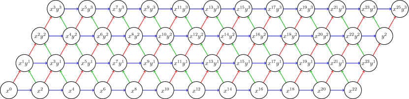
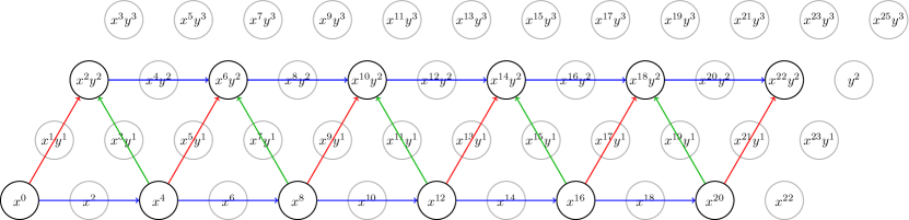
Figure 3: Signal model of a directed hexagonal lattice for $N=4$. The boundary conditions are omitted. Shifts of $X$ are blue, shifts of $Y$ are red, and shifts of $Z$ are green colored.

Figure 4: Sublattice of the hexagonal lattice corresponding to the transversal element $1$.

From the structure of the submodule and the transversal it is obvious that the basis change to the induced module is a permutation matrix, hence is sparse.

None of the elements of $\mathsf{V}(\langle\;y^{N}-1,x^{3N}-y^{N/2}{\;}\rangle)$ gets mapped to zero by an element of the transversal. The preimage of each point of $V(\langle\;y^{N/2}-1,x^{3N/2}-y^{N/4}{\;}\rangle)$ consists at most of four points of $V(\langle\;y^{N}-1,x^{3N}-y^{N/2}{\;}\rangle)$. Hence each row of $M$ has at most $4$ non-zero entries, thus $M$ has $O(n)$ entries and is sparse. Thus by Prop. 3 we have a fast algorithm.

Remark 3

In Pueschel.Roetteler:2005a a signal model for the directed quincunx lattice was introduced. This signal model used a basis similar to the one we used in Example 2. These examples show that the algebra action on the module is indeed crucial for the signal model.

3 Orthogonal polynomials and orthogonal transforms

Orthogonal polynomials are at the heart of numerical mathematics. In this section we recall some properties of them, focusing on the multivariate case. Especially interesting for their usage in algebraic signal processing are the three-term recurrence relations and the Christoffel-Darboux formula. Since the theory of multivariate orthogonal polynomials relies on a formulation not in special bases but spaces of polynomials of the same degree, we introduce a notion of equivalence of signal models to capture that ambiguity. Then the multivariate Christoffel-Darboux formula is used to derive a multivariate version of the Gauß-Jacobi procedure for finding orthogonal Fourier transforms.

We then recall the notion of Gaussian cubature. Whilst in the univariate case Gaussian cubature formulae always exist, this is not the case in the multivariate setting. Indeed there are few domains known for which such a formula can be stated. We show that the existence of a orthogonal Fourier transform for a signal model with orthogonal polynomials as basis is implied by the existence of a Gaussian cubature.

In this section we denote by $x=(x_{1},\dots,x_{d})$. Denote by $\Pi_{n}^{d}$ the space of polynomials in $d$ variables of degree at most $n$. Let $\langle\,\cdot\,,\,\cdot\,\rangle$ be an inner product on $\Pi^{d}$. The space of orthogonal polynomials of degree $n$ is denoted by

$$\mathcal{V}_{n}^{d}=\{p\in\Pi_{n}^{d}\;|\;\langle p,q\rangle=0\text{ for all }q\in\Pi_{n-1}^{d}\}.$$ (29)

If the inner product is given by $\langle f,g\rangle=\int_{\mathbb{R}^{d}}f(x)g(x)\mathop{}\!\mathrm{d}\mu(x)$ such that the measure $\mu$ has support with non-empty interior, then

$$\dim\mathcal{V}_{n}^{d}=\binom{n+d-1}{n}=r_{n}^{d}.$$ (30)

Let $\mathbb{P}_{n}=(P_{\alpha}^{n})_{|\alpha|=n}$, with $\alpha\in\mathbb{N}_{0}^{d}$ a multi-index, denote a basis of $\mathcal{V}_{n}^{d}$ and let $\mathbb{P}_{-1}(x)=0$. There exist unique matrices $A_{n,i}$ of size $r_{n}^{d}\times r_{n+1}^{d}$, $B_{n,i}$ of size $r_{d}^{d}\times r_{n}^{d}$, and $C_{n,i}$ of size $r_{n}^{d}\times r_{n-1}^{d}$ such that one has the three-term recurrence relation

$$x_{i}\mathbb{P}_{n}(x)=A_{n,i}\mathbb{P}_{n+1}(x)+B_{n,i}\mathbb{P}_{n}(x)+C_{n,i}\mathbb{P}_{n-1}.$$ (31)

The matrices $A_{n,i}$ and $C_{n,i}$ are of full rank. If the $\mathbb{P}_{n}$ are even orthonormal one has $C_{n,i}=A_{n-1,i}^{\top}$.

From this three-term recurrence relation Xu deduced a multivariate Christoffel-Darboux formula Xu:1993a , which reads

$$\begin{split}&\sum_{k=0}^{n}\mathbb{P}_{k}^{\top}(x)H_{k}^{-1}\mathbb{P}_{k}(y)\\ &=\begin{cases}\frac{(A_{n,i}\mathbb{P}_{n+1}(x))^{\top}H_{n}^{-1}\mathbb{P}_{n}(y)-\mathbb{P}_{n}^{\top}(x)H_{n}^{-1}A_{n,i}\mathbb{P}_{n+1}(y)}{x_{i}-y_{i}}&\text{if }x\not=y\\ \mathbb{P}_{n}^{\top}(x)H_{n}^{-1}A_{n,i}\frac{\partial}{\partial x_{i}}\mathbb{P}_{n+1}(x)-(A_{n,i}\mathbb{P}_{n+1}(x))^{\top}H_{n}^{-1}\frac{\partial}{\partial x_{i}}\mathbb{P}_{n}(x)&\text{if }x=y,\end{cases}\end{split}$$ (32)

where the $H_{k}$ are invertible, symmetric matrices such that $B_{k,i}H_{k}$ is symmetric and one has $A_{k,i}H_{k+1}=H_{k}C_{k+1,i}^{\top}$. The matrices $H_{k}$ are given as $H_{k}=\mathcal{L}(\mathbb{P}_{k}\mathbb{P}_{k}^{\top})$, with $\mathcal{L}(f)=\int_{\mathbb{R}^{d}}f(x)\mathop{}\!\mathrm{d}\mu(x)$. Note that the value of the sum $\sum_{k=0}^{n}\mathbb{P}_{k}^{\top}(x)H_{k}^{-1}\mathbb{P}_{k}(y)$ is independent on the actual choice of the bases $\mathbb{P}_{k}$ in the $\mathcal{V}_{k}^{d}$. This follows from the equality $\mathbb{P}^{\top}\mathcal{L}(\mathbb{P}_{k}\mathbb{P}_{k}^{\top})\mathbb{P}=\mathbb{Q}^{\top}\mathcal{L}(\mathbb{Q}_{k}\mathbb{Q}_{k}^{\top})\mathbb{Q}$ for any choice of bases $\mathbb{P},\mathbb{Q}$ in $\mathcal{V}_{k}^{d}$, cf. Xu:1993a . Note that even though it appears from the right-hand side of the formula that it depends on the choice of index $i$, the left-hand side shows that its value actually is independent of $i$.

Another nice property of orthogonal polynomials is that their common zeros are particular well-behaved. Recall that a common zero of $\mathbb{P}_{n}$ is a zero of all the $P_{\alpha}^{n}$ in $\mathbb{P}_{n}$. All common zeros of $\mathbb{P}_{n}$ are real, distinct and simple, i.e. at least one $\tfrac{\partial}{\partial x_{i}}\mathbb{P}_{n}$ does not vanish and the set $\mathbb{P}_{n}$ has at most $\dim\Pi_{n-1}^{d}$ common zeros, cf. Xu:2017a .

We now adopt the point of view, that orthogonality does not hold in terms of particular bases of $\mathcal{V}_{n}^{d}$ but in terms of the subspaces $\mathcal{V}_{n}^{d}$, to algebraic signal models.

Definition 1

Two signal models $(\mathscr{A},M,\Phi_{1})$ and $(\mathscr{A},M,\Phi_{2})$, with bases of the modules given by sets of orthogonal polynomials $\mathbb{P}_{1}$ and $\mathbb{P}_{2}$, are called insignificantly different if $\mathbb{P}_{1}$ and $\mathbb{P}_{2}$ are orthogonal with respect to the same positive definite linear functional.

From a signal processing perspective it is interesting when one can obtain an orthogonal transform. In the univariate case the Gauß-Jacobi procedure Yemini.Pearl:1979a shows that one can always obtain an orthogonal transform if the basis of the signal module consists of orthogonal polynomials. In the multivariate case one has to assume an additional condition on the number of common zeros of the orthogonal polynomials.

Theorem 3.1

Consider a signal model with underlying variety $V=\mathsf{V}(\langle\;\mathbb{P}_{n}{\;}\rangle)$ with $|V|=\dim\Pi_{n-1}^{d}$ and let the basis of the module be given by $(\mathbb{P}_{i})_{i=0}^{n-1}$. Then there exists an insignificantly different signal model with orthogonal Fourier transform.

Proof

If the variety of the signal model consists of the nodes of such a Gaussian cubature formula, the underlying variety $\mathsf{V}$ consists of common zeros of all $\mathbb{P}_{n}$. We can assume that all the $(\mathbb{P}_{i})_{i=0}^{n-1}$ are orthonormal since this choice only leads to an insignificantly different signal model. Then the product of the Fourier transform matrices for this signal model $\mathcal{F}^{\top}\cdot\mathcal{F}$ has entries of the form $\sum_{k=0}^{n-1}\mathbb{P}_{k}(\alpha)^{\top}\mathbb{P}_{k}(\beta)$ for $\alpha,\beta\in\mathsf{V}$. Now by the Christoffel-Darboux formula (32) the entries not on the diagonal are zero since $\mathbb{P}_{n}(\alpha)=0$ for each $\alpha\in\mathsf{V}$. On the other hand the diagonal entries have the form

$$\mathbb{P}_{n-1}^{\top}(\alpha)A_{n-1,i}\tfrac{\partial}{\partial x_{i}}\mathbb{P}_{n}(\alpha).$$

Since the common zeros of $\mathbb{P}_{n}$ are simple, i.e. at least one partial derivative of $\mathbb{P}_{n}$ is not zero, cf. (Xu:2017a, , Thm. 2.13), we can invert the diagonal entries, which do not depend on $i$. If we now choose in the one-dimensional, irreducible component belonging to $\alpha$ the basis $\Big{(}\sqrt{\mathbb{P}_{n-1}^{\top}(\alpha)A_{n-1,i}\tfrac{\partial}{\partial x_{i}}\mathbb{P}_{n}(\alpha)}\Big{)}$ we obtain an orthogonal Fourier transform $\mathcal{F}^{\mathsf{orth}}$. This can be seen as follows. Consider the diagonal matrix

$$\sqrt{D}=\mathsf{diag}\left(1\Big{/}\sqrt{\mathbb{P}_{n-1}^{\top}(\alpha)A_{n-1,i}\tfrac{\partial}{\partial x_{i}}\mathbb{P}_{n}(\alpha)}\;\bigg{|}\;\alpha\in\mathsf{V}\right).$$

Then $\mathcal{F}^{\mathsf{orth}}=\sqrt{D}\mathcal{F}$, hence we obtain from the above discussion

$$\mathcal{F}^{\mathsf{orth},\top}\cdot\mathcal{F}^{\mathsf{orth}}=\mathcal{F}^{\top}\sqrt{D}\sqrt{D}\mathcal{F}=D\mathcal{F}^{\top}\mathcal{F}=\mathbbm{1},$$

since diagonal matrices commute with all matrices. The theorem is proven. ∎

Now the condition that one has $|\mathsf{V}(\langle\;\mathbb{P}_{n}{\;}\rangle)|=\dim\Pi_{n-1}^{d}$ is very restrictive. Indeed it is the same condition as for the existence of a Gaussian cubature formula and there are few multi-dimensional regions known for which Gaussian cubature formulas exist.

Recall that a cubature formula for the measure $\mu$ is a finite sum that approximates integrals $\int_{\mathbb{R}^{d}}\,\cdot\,\mathop{}\!\mathrm{d}\mu$. If one has

$$\int_{\mathbb{R}^{d}}f(x)\mathop{}\!\mathrm{d}\mu=\sum_{k=1}^{N}w_{k}f(x_{k}),$$ (33)

with weights $w_{k}\in\mathbb{R}$ and nodes $x_{k}\in\mathbb{R}^{d}$, for all $f\in\Pi_{2n-1}^{d}$ and this does not hold for at least one element of $\Pi_{2n}^{d}$, the cubature is said to be of degree $2n-1$. For the number of nodes $N$ one has

$$N\geq\dim\Pi_{n-1}^{d}$$ (34)

and if the bound is reached the cubature formula is called Gaussian. A Gaussian cubature formula exists if and only if $\mathbb{P}_{n}$ has $\dim\Pi_{n-1}^{d}$ common zeros Mysovskikh:1976a . The nodes of the cubature formula are then precisely the common zeros of $\mathbb{P}_{n}$. Hence if there exists a Gaussian cubature formula one can ensure the existence of an orthogonal transform for a corresponding signal model. Now the existence of Gaussian cubature formulas is rare, the first class of examples in any dimension has been described in Berens.Schmid.Xu:1995a and other examples have been discussed in Li.Sun.Xu:2008 ; Moody.Patera:2011 ; Hrivnak.Motlochova.Patera:2016 . Thus the applicabilty of the multivariate Gauss-Jacobi procedure is restricted to certain special cases. One of these special cases will be investigated in the next section.

4 FFT for weight lattices

While directed signals are of interest in the analysis of time-dependent data like time-series, undirected signals are considered in the analysis of space-dependent data like images.

In the one-dimensional case the undirected counterparts to the directed discrete Fourier transform are the discrete sine and cosine transforms. In Pueschel.Moura:2008c the signal models and fast transforms for all 16 discrete sine and cosine transforms were deduced in algebraic signal processing. In this section undirected signal models and their fast transforms for a special class of lattices, the weight lattices of semi-simple Lie groups, are derived. The approach mimics the ansatz of Pueschel.Moura:2008c for the DCT-3. This ansatz relies on Chebyshev polynomials of the first kind. This family of polynomials is one of the only two in one variable obeying the decomposition property.

We start by recalling the ansatz for DCT-3. Consider the Chebyshev polynomials of the first kind $T_{n}(\cos\theta)=\cos n\theta$. They obey the shift property

$$xT_{n}(x)=\tfrac{1}{2}(T_{n-1}(x)+T_{n+1}(x)).$$ (35)

Consider the signal model with filter algebra $\mathscr{A}=\mathbb{C}[x]\big{/}\langle\;T_{n}{\;}\rangle$,the regular module $M=\mathscr{A}$ as signals and $\Phi\colon s\mapsto\sum_{i}s_{i}T_{i}$ determining the Chebyshev polynomials as basis. By (35) the visualization of the signal model is an undirected lattice as illustrated in Fig. 5.

Figure 5: The visualization of the discrete cosine transform signal model.

The choice of the basis $\{T_{0},T_{1},\ldots,T_{n}\}$ leads to the discrete cosine transform of type 3. The other types of discrete cosine and sine transforms can be obtained by a combination of different choices of kinds of Chebyshev polynomials and roots of them, cf. Pueschel.Moura:2003a .

One particular nice property of the Chebyshev polynomials is the decomposition property

$$T_{k\cdot n}(x)=T_{n}(T_{k}(x)).$$ (36)

Up to similarity the Chebyshev polynomials and the monomials $x^{n}$ are the only polynomials in one variable subject to the decomposition property.

By the above considerations it is natural to search for several variable analogues of the Chebyshev polynomials. Fortunately there is a rather mature theory of multivariate Chebyshev polynomials available Hoffman.Withers:1988a which has an intimate connection to Lie theory. This generalization is based on the stretching and folding property, a geometric interpretation of the decomposition, of the one-dimensional Chebyshev polynomials, i.e. the map

$$\cos^{-1}\circ T_{n}\circ\cos$$ (37)

stretches the interval $[0,1]$ $n$-times and folds it back at the integers. In Hoffman.Withers:1988a it was shown that the foldable figures in higher dimensions are in one-to-one correspondence to the Weyl groups of root systems.

For the correct generalisation of the appearing components we need to recall some definitions and tools from Lie theory. This will include an explanation of the domain of $\theta$ and the index set, aswell.

The first definition we need is that of a root system and its dual, the coroot system. Root systems were introduced by Killing for the classification of the complex, simple Lie algebras Killing:1888a .

Definition 2

A crystallographic root system in a finite-dimensional euclidean space $(\mathbb{R}^{d},\langle\,\cdot\,,\,\cdot\,\rangle)$ is a finite set $R$ of non-zero vectors, the so-called roots, which span $\mathbb{R}^{d}$ subject to the conditions

1. $r\cdot a\in R$ then $r=\pm 1$ for all $\alpha\in R$,

2. closedness under reflections through the hyperplanes perpendicular to the roots, i.e.

   $$\sigma_{\alpha}(\beta)=\beta-2\frac{\langle\alpha,\beta\rangle}{\langle\alpha,\alpha\rangle}\alpha\in R$$ (38)

   for all $\alpha,\beta\in R$,

3. for any $\alpha,\beta\in R$ we have $2\tfrac{\langle\alpha,\beta\rangle}{\langle\alpha,\alpha\rangle}\in\mathbb{Z}$.

The set of integer linear combinations of the roots is termed root lattice

$$Q=\operatorname{\mathrm{span}}_{\mathbb{Z}}\{\alpha\in R\}\subseteq\mathbb{R}^{d}.$$ (39)

The coroot of a root $\alpha\in R$ is

$$\alpha^{\vee}=\frac{2}{\langle\alpha,\alpha\rangle}\alpha.$$ (40)

The coroots form a root system which is denoted by $R^{\vee}$. The coroot lattice $Q^{\vee}$ is the $\mathbb{Z}$-span of the coroots

There are at most two different root lengths for an irreducible root system, i.e. one which is not a combination of root systems with mutually orthogonal spaces. The irreducible root systems can be classified using Coxeter-Dynkin diagrams. There are four infinite series $A_{n},B_{n},C_{n},D_{n}$ and five exceptional root systems $E_{6},E_{7},E_{8},F_{4},G_{2}$, cf. Fig. 6.

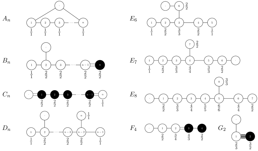
Figure 6: Affine Coxeter-Dynkin diagrams for the reduced, crystallographic root systems. The dotted node corresponds to the lowest root $-\alpha_{0}$, the numbered nodes to the simple roots $\alpha_{i}$. Open circles are long roots, while filled nodes indicate short roots. The marks and comarks are shown below the nodes as $\tfrac{m_{i}}{m_{i}^{\vee}}$. The angle between two roots depends on the multiplicity $k$ of the edge between them and is given as $4\cos^{2}\theta=k$ and $\cos\theta\leq 0$, i.e. $\tfrac{\pi}{2},\tfrac{2\pi}{3},\tfrac{3\pi}{4},\tfrac{5\pi}{6}$ with length ratio being arbitrary, $1,\sqrt{2},\sqrt{3}$ for $k=0,1,2,3$, respectively.

One can choose a basis $\Delta=\{\alpha_{1},\dots,\alpha_{d}\}\subseteq R$ of the root system such that one has $\alpha=\sum_{i=1}^{d}c_{j}\alpha_{j}$ with all $c_{j}\in\mathbb{Z}$ of the same sign. The $\alpha_{i}$ are called simple roots. The simple roots divide the root system into positive roots $R^{+}$ and negative roots $R^{-}$. The simple roots introduces a partial order on the roots, aswell. The partial order is defined by $\lambda\succeq\mu$ if the expansion of $\lambda-\mu$ in simple roots has non-negative coefficients only. Then $\lambda$ is called higher than $\mu$. The highest root is

$$\alpha_{0}=m_{1}\alpha_{1}+\dots+m_{d}\alpha_{d},$$ (41)

with positive integers $m_{i}$. The $m_{i}$ are called the marks of the root system. The marks of the coroot system are called the comarks of the initial root system and denoted by $m_{1}^{\vee},\dots,m_{d}^{\vee}$.

The Weyl group of a root system $R$ is the group generated by the reflections

$$W=\langle\;\sigma_{\alpha}\;|\;\alpha\in R{\;}\rangle.$$ (42)

The $\mathbb{Z}$-dual of $Q$ is the coweight lattice $P^{\vee}$, while the $\mathbb{Z}$-dual of $Q^{\vee}$ is the weight lattice $P$. The generators of $P$ are the fundamental weights $\omega_{j}$ and the generators of $P^{\vee}$ are the fundamental coweights $\omega_{j}^{\vee}$.

The coroot lattice acts on $\mathbb{R}^{d}$ by translation and the affine Weyl group is the semi-direct product

$$W_{\text{aff}}=W\ltimes Q^{\vee}.$$ (43)

The simplex $F=\mathbb{R}^{d}\big{/}Q^{\vee}$ tiles $\mathbb{R}^{d}$ under the action of the affine Weyl group and is called the fundamental Weyl chamber. One can use the fundamental coweights to describe the fundamental Weyl chamber as convex hull

$$F=\mathsf{conv}\left\{0,\frac{\omega_{1}^{\vee}}{m_{1}},\dots,\frac{\omega_{d}^{\vee}}{m_{d}}\right\}.$$ (44)

This fundamental region replaces the interval $[0,1]$ as stretching and folding region for multivariate Chebyshev polynomials. In Fig. 7 the root systems of type $A_{2}$ and $C_{2}$ are shown together with the simple scaled coweights and the fundamental domains.

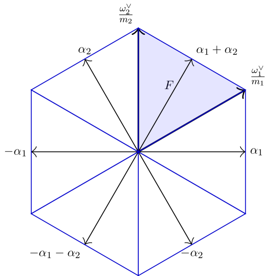
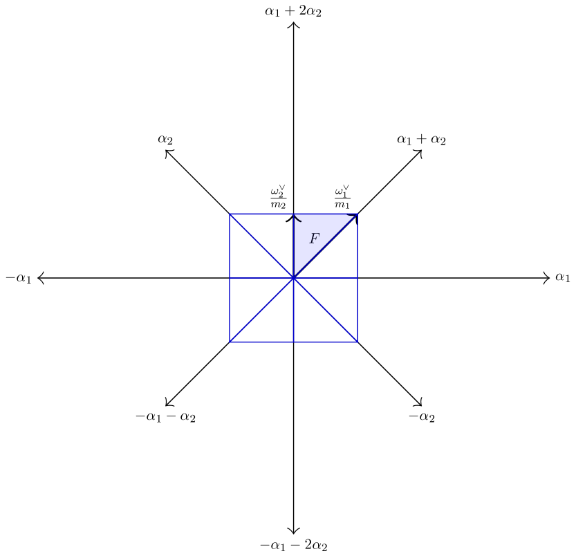
Figure 7: The root systems of type $A_{2}$ (upper) and $C_{2}$ (lower) together with the fundamental region $F$ (shaded region) and the image of $F$ under the action of the Weyl group.

The dual pairing $(\,\cdot\,,\,\cdot\,)\colon P\times\mathbb{R}^{d}\big{/}Q^{\vee}\longrightarrow\mathbb{C}$ is given by

$$(\lambda,\theta)=\exp(2\pi\mathrm{i}\langle\lambda,\theta\rangle).$$ (45)

The Weyl group, which is isomorphic to a group of integer matrices, acts on $P$ and $\mathbb{R}^{d}\big{/}Q^{\vee}$. Symmetrization of the dual pairing with respect to the corresponding Weyl group now leads to the definition of multivariate Chebyshev polynomials.

Definition 3

Let $W$ be a Weyl group of a root system $R$ with weight lattice $P$ and coroot lattice $Q^{\vee}$. The multivariate Chebyshev polynomials of the first kind of weight $\lambda\in P$ is

$$T_{\lambda}(x_{1},\dots,x_{d})=\frac{1}{|W|}\sum_{w\in W}(\lambda,w\theta),$$ (46)

for $\theta\in F$. The multivariate Chebyshev polynomials are polynomials in the variables

$$x_{k}=(\omega_{k},\theta),$$ (47)

with $\theta\in F$.

Indeed, for the Weyl group $W(A_{1})$ of type $A_{1}$ one gets back the original definition of Chebyshev polynomials, as the root system is then $R_{A_{1}}=\{1,-1\}$ and is equal to the coroot lattice, the only simple root is $\{1\}$, the Weyl group is $W(A_{1})=\{1,-1\}$, the root and coroot lattice is $\mathbb{Z}$, the weight lattice is $P=\mathbb{Z}$. This leads to $F=[0,1]$ and $T_{n}(x)=(n,\theta)=\tfrac{1}{2}(\exp(2\pi\mathrm{i}n\theta)+\exp(-2\pi\mathrm{i}n\theta)=\cos(n\theta)$.

The simplex $F$ gets transformed under the variable change $x_{k}=(\omega_{k},\theta)$ to a cusped region. For example in case of the root system $A_{2}$ the fundamental region $F$ is an equilateral triangle which gets transformed to a deltoid under $(x_{1},x_{2})$. In Fig. 8 the cusped regions for the irreducible two-dimensional root systems are shown.

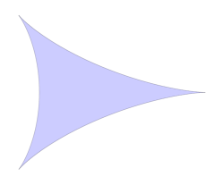
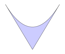
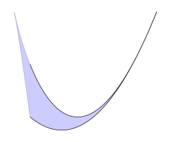
Figure 8: The image of the fundamental region $F$ under the variable change in case of $A_{2}$, $C_{2}$, and $G_{2}$, respectively.

The multivariate Chebyshev polynomials share many of the nice properties the univariate ones posess. We list the properties used in the sequel.

Proposition 6

The multivariate Chebyshev polynomials associated to a Weyl group $W$ are subject to

1. invariance with respect to the action of the Weyl group on the weight indices

   $$T_{w\lambda}=T_{\lambda}$$ (48)

   and invariance with respect to the affine Weyl group on the argument in the fundamental domain

   $$T_{\lambda}((\omega_{1},w\theta),\dots,(\omega_{d},w\theta))=T_{\lambda}((\omega_{1},\theta),\dots,(\omega_{d},\theta)),$$ (49)

2. the shift property

   $$T_{\lambda_{1}}T_{\lambda_{2}}=\tfrac{1}{|W|}\sum_{w\in W}T_{\lambda_{1}+w\lambda_{2}},$$ (50)

3. the decomposition property

   $$T_{k\lambda}=T_{\lambda}(T_{k\omega_{1}},\dots,T_{k\omega_{d}})$$ (51)

   for $\lambda\in P$ and $k\in\mathbb{Z}$.

The properties i.) and ii.) of Prop. 6 yield a recursion relation if one uses the shift relation with the $x_{k}=(\omega_{k},\theta)$.

The standard grading on the Chebyshev polynomials is insufficient for our purposes as then, except for the case $A_{n}$, we do not obtain the Gröbner basis property for $T_{n\omega_{1}},\dots,T_{n\omega_{d}}$. Replacing the standard degree with the m-degree introduced in Moody.Patera:2011 solves this issue. The m-degree weights the weights with the comarks.

Definition 4

Let $\lambda\in P$ then its m-degree is

$$\operatorname{{\mathrm{deg}}_{m}}(\lambda)=\langle\lambda,\alpha_{0}^{\vee}\rangle.$$ (52)

A monomial $x_{1}^{\lambda_{1}}\dots x_{d}^{\lambda_{d}}$ is then of m-degree $\operatorname{{\mathrm{deg}}_{m}}(\lambda)=\operatorname{{\mathrm{deg}}_{m}}((\lambda_{1},\dots,\lambda_{d}))$.

The $\mathrm{m}$-graded lexicographical ordering on the monomials is defined by ordering the monomials with respect to $\operatorname{{\mathrm{deg}}_{m}}$ and then breaking ties by the lexicographical order on the variables.

In case of type $A_{n}$ all marks are equal to $1$, so in these cases the m-degree coincides with the standard degree. The leading monomial of the Chebyshev polynomial $T_{\lambda}$ with respect to the m-graded lexicographical ordering is $x_{1}^{\lambda_{1}}\dots x_{d}^{\lambda_{d}}$. By the recursion relations obtained from the shift relation the leading monomials with respect to m-graded lexicographical ordering of the polynomials $T_{n\omega_{1}},\dots,T_{n\omega_{d}}$ are disjoint. Hence they form a Gröbner basis for the ideal they generate.

Example 3

The proposed algorithm for $A_{2}$, based on Theorem 2.1, is an alternative to the one proposed in Pueschel.Roetteler:2008 , which relied on a version of Theorem 2.2. The shift relation reads in this case

$$\begin{split}x_{1}T_{\lambda_{1},\lambda_{2}}&=\tfrac{1}{3}\left(T_{\lambda_{1}+1,\lambda_{2}}+T_{\lambda_{1},\lambda_{2}-1}+T_{\lambda_{1}-1,\lambda_{2}+1}\right)\\ x_{2}T_{\lambda_{1},\lambda_{2}}&=\tfrac{1}{3}\left(T_{\lambda_{1},\lambda_{2}+1}+T_{\lambda_{1}-1,\lambda_{2}}+T_{\lambda_{1}+1,\lambda_{2}-1}\right).\end{split}$$ (53)

A set of sufficient starting conditions for running the recursion is

$$\begin{split}T_{0,0}&=1,\\ T_{1,0}&=x,\\ T_{0,1}&=y,\\ T_{1,1}&=\tfrac{3}{2}xy-\tfrac{1}{2}.\end{split}$$ (54)

We consider the signal model consisting of

$$\begin{split}\mathscr{A}&=\mathbb{C}[x,y]\big{/}\langle\;T_{0,n},T_{n,0}{\;}\rangle,\\ M&=\mathscr{A}\text{ (as regular module)},\\ \end{split}$$ (55)

and

$$\begin{split}\Phi\colon\mathbb{C}^{n^{2}}&\longrightarrow M,\\ \Phi(s)&=\sum_{k,\ell=0}^{n}s_{k,\ell}T_{k,\ell}.\end{split}$$ (56)

The visualization unveils the hexagonal lattice underlying this signal model, cf. Fig. 9, obtained from the shift relations (53).

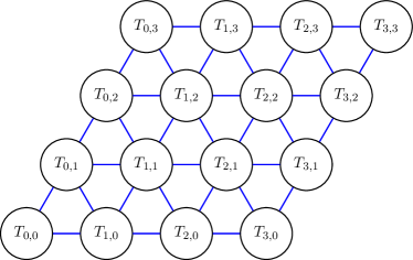
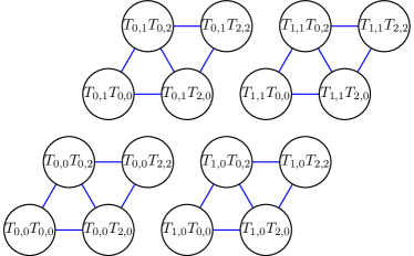
Figure 9: Visualization of the signal model for Chebyshev polynomials of type $A_{2}$, a directed hexagonal lattice (left), and after representing the module as induction (right).

In Pueschel.Roetteler:2008 the $n^{2}$ common zeros of $T_{n,0}$ an $T_{0,n}$ were described elementary. We propose a geometric description of the common zeros, as this shows the geometric mechanisms underlying the decomposition more clearly. The preimage of $0$ in the $x-y$-Domain is $\frac{1}{3}\omega_{1}^{\vee}+\frac{1}{3}\omega_{2}^{\vee}$. Through the stretching-and-folding property and the condition that the common zeros be in the fundamental domain $F$ one obtains

$$\begin{split}\mathsf{V}(\langle\;T_{n,0},T_{0,n}{\;}\rangle)&=\{\frac{1+3j}{3n}\omega_{1}^{\vee}+\frac{1+3k}{3n}\omega_{2}^{\vee}\;|\;2+3(j+k)<3n\}\\ &\quad\cup\{\frac{2+3j}{3n}\omega_{1}^{\vee}+\frac{2+3k}{3n}\omega_{2}^{\vee}\;|\;4+3(j+k)<3n\},\end{split}$$ (57)

with $j,k=0,\dots,n-1$. For each $\alpha\in\mathsf{V}(\langle\;T_{r,0},T_{0,r}{\;}\rangle)$ one has $|\mathsf{V}(\langle\;T_{m,0}-\alpha_{1},T_{0,m}-\alpha_{2}{\;}\rangle)|=m^{2}$. The geometric mechanism of the distribution of the common zeros is illustrated in Fig. 10.

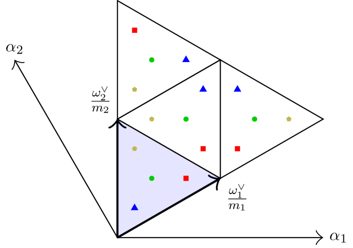
Figure 10: The four classes of common zeros of for the skew transforms in case $n=2\cdot 2$. The common zeros of $\langle\;T_{4,0},T_{0,4}{\;}\rangle$ are shown after being stretched by a factor of $2$. The action of the affine Weyl group, folding the stretched triangle back to the fundamental domain, is indicated. The different colors indicate which common zeros of $\langle\;T_{4,0},T_{0,4}{\;}\rangle$ are common zeros of which $\langle\;T_{2,0}-\alpha_{1},T_{0,2}-\alpha_{2}{\;}\rangle$.

Since for $n=r\cdot m$ one thus has $|\mathsf{V}(\langle\;T_{n,0},T_{0,n}{\;}\rangle)|=|\mathsf{V}(\langle\;T_{r,0},T_{0,r}{\;}\rangle)|\cdot|\mathsf{V}(\langle\;T_{m,0},T_{0,m}{\;}\rangle)|$ and all the subalgebras $\mathbb{C}[x,y]\big{/}\langle\;T_{m,0}-\alpha_{1},T_{0,m}-\alpha_{2}{\;}\rangle$ are of equal dimension, by Prop. 5 any basis of $\mathbb{C}[x,y]\big{/}\langle\;T_{r,0},T_{0,r}{\;}\rangle$ is a transversal of $\mathbb{C}[x,y]\big{/}\langle\;T_{m,0},T_{0,m}{\;}\rangle$. Since the basis change between the basis $(T_{0,0},\dots,T_{n,n})$ and the induction basis is sparse, see App. A.1 for the concrete form, by Prop. 3 the Theorem 2.1 yields a $O(n^{2}\log(n))$ algorithm. This is substantially faster than the naive $O(n^{4})$-approach.

Example 4

In case $C_{2}$ the shift relation is

$$\begin{split}x_{1}\cdot T_{k,\ell}&=\tfrac{1}{4}\left(T_{k+1,\ell}+T_{k-1,\ell}+T_{k-1,\ell+2}+T_{k+1,\ell-2}\right),\\ x_{2}\cdot T_{k,\ell}&=\tfrac{1}{4}\left(T_{k,\ell+1}+T_{k,\ell-1}+T_{k-1,\ell+1}+T_{k+1,\ell-1}\right).\end{split}$$ (58)

A set of sufficient starting conditions for running the recurrence relation is

$$\begin{split}T_{0,0}&=1,\\ T_{1,0}&=x_{1},\\ T_{0,1}&=x_{2},\\ T_{1,1}&=2x_{1}x_{2}-x_{1}.\end{split}$$ (59)

The weight vector for the total $m$-degree lexicographical ordering of the monomials is $(1,2)$. That is $\operatorname{{\mathrm{deg}}_{m}}(x_{1})=1$ and $\operatorname{{\mathrm{deg}}_{m}}(x_{2})=2$.

Denote by $\mathbb{T}_{n}=\{T_{k,\ell}\;|\;k+\ell=n\}$. Then one has a three-term recurrence of the form

$$x_{i}\mathbb{T}_{k}=A_{k,i}\mathbb{T}_{k+1}+B_{k,i}\mathbb{T}_{k}+C_{k,i}\mathbb{T}_{k-1},$$ (60)

were the matrices $A_{k,i},B_{k,i},$ and $C_{k,i}$ can be deduced from the shift relations (58). For example for the $x_{1}$ shift one obtains

$$A_{k,1}=\begin{bmatrix}0&1/2&0&\dots&&0\\ 1/4&0&1/4&0&\dots&0\\ 0&\ddots&\ddots&\ddots&&\vdots\\ \dots&0&1/4&0&1/4&0\\ 0&\dots&0&1/2&0&1/4\end{bmatrix},$$ (61)

$$B_{k,1}=\begin{bmatrix}0&\dots&&0\\ \vdots&\ddots&&\vdots\\ 0&\dots&0&0\\ 0&\dots&1/4&0\\ 0&\dots&0&0\end{bmatrix},$$ (62)

and

$$C_{k,1}=\begin{bmatrix}0&1/2&0&\dots&0\\ 1/4&0&1/4&\ddots&\vdots\\ 0&\ddots&\ddots&\ddots&0\\ &&1/4&0&1/4\\ \vdots&&0&1/4&0\\ 0&\dots&&0&1/4\end{bmatrix},$$ (63)

with special case $B_{1,1}=\begin{bmatrix}1/2&0\\ 0&0\end{bmatrix}$. The Christoffel-Darboux formula (32) can be realized using the matrices $H_{0}=\tfrac{1}{2}$ and $H_{k}=\mathsf{diag}(\tfrac{1}{8},\tfrac{1}{16},\dots,\tfrac{1}{16},\tfrac{1}{8})$.

We consider the signal model consisting of

$$\begin{split}\mathscr{A}&=\mathbb{R}[x_{1},x_{2}]\big{/}\langle\;\mathbb{T}_{n}{\;}\rangle,\\ M&=\mathscr{A}\text{ (as regular module)},\\ \end{split}$$ (64)

and

$$\begin{split}\Phi\colon\mathbb{R}^{\frac{n(n+1)}{2}}&\longrightarrow M,\\ \Phi(s)&=\sum_{k+\ell<\frac{n(n+1)}{2}}s_{k,\ell}T_{k,\ell}.\end{split}$$ (65)

The signal model has a visualization, which resembles a triangle, cf. Fig. 11.

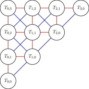
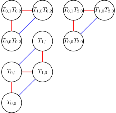
Figure 11: Visualization of the signal model for Chebyshev polynomials of type $C_{2}$ on the left. The shifts of $x_{1}$ are blue and the shifts of $x_{2}$ are red colored. On the right the decomposed lattice after the basis change is shown.

In Seifert.Hueper:2018b we used an elementary description of the common zeros of $\mathbb{T}_{n}$. Here we present again a more geometric point of view, using the coweights. That is the common zeros are given as

$$\mathsf{V}(\langle\;\mathbb{T}_{n}{\;}\rangle)=\Big{\{}\tfrac{2j+1}{2n}\omega_{1}^{\vee}+\tfrac{k}{2n}\omega_{2}^{\vee}\;\Big{|}\;j,k=0,\dots,n-1,\;j+k<n\}.$$ (66)

This results in $\frac{n(n+1)}{2}$ common zeros.

We derive a fast algorithm in case $n=2\cdot m$. Since for $n=2\cdot m$ it is $\frac{n(n+1)}{2}\not=\frac{2(2+1)}{2}\cdot\frac{m(m+1)}{2}$ one does not get an induction via the decomposition.

Due to the decomposition property 6, iii.), the map

$$(x_{1},x_{2})\mapsto(T_{2,0}(x_{1},x_{2}),T_{0,2}(x_{1},x_{2}))$$ (67)

maps the variety $\mathsf{V}(\mathbb{T}_{n})$ to the variety $\mathsf{V}(\mathbb{T}_{m})$. The map

$$(x_{1},x_{2})\mapsto(T_{m,0}(x_{1},x_{2}),T_{0,m}(x_{1},x_{2})$$ (68)

stretches the fundamental region $F$ by a factor of $m$ and folds it back under the affine Weyl group. After the stretching operation one obtains $m^{2}$ copies of the fundamental region. Thus if $\left(\frac{k}{2n},\frac{j}{4n}\right)$ is in the interior of $F$ one obtains $m^{2}$ common zeros. If $\left(\frac{k}{2n},\frac{j}{4n}\right)$ is on the boundary of $F$, that is $k=0$, always two of the copies of $F$ in the interior of the stretched region share these common zeros. Hence in this case one only obtains $\frac{m(m+1)}{2}$ common zeros. Of the common zeros of $\mathbb{T}_{2}$ there is one in the interior and two on the boundary. Since these are the images under the stretching and folding operation one obtains two subalgebras with $\frac{m(m+1)}{2}$ common zeros and one subalgebra with $m^{2}$ common zeros.

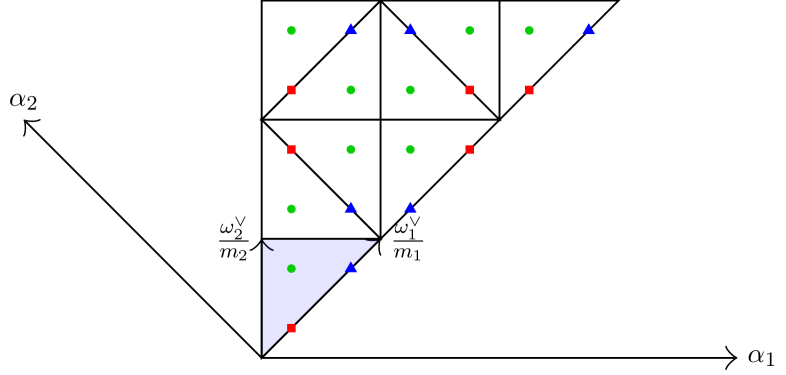
Figure 12: The three classes of common zeros of for the skew transforms in case $n=2\cdot 3$. The common zeros of $\mathbb{T}_{6}$ are shown after being stretched by a factor of $3$.The action of the affine Weyl group, folding the stretched triangle back to the fundamental domain, is indicated. The different colors indicate which common zeros of $\langle\;T_{6,0},T_{0,6}{\;}\rangle$ are common zeros of which $\langle\;T_{3,0}-\alpha_{1},T_{0,3}-\alpha_{2}{\;}\rangle$.

Since the basis change obtained in App. A.2 is sparse, we obtain a fast $O(n^{2}\log n)$ algorithm by Theorem 2.2.

Since the number of common zeros of $\mathbb{T}_{n}$ equals $\dim\Pi_{2}^{n-1}$ Theorem 3.1 implies the existence of an orthogonal transform. Denote the diagonal matrix with inverted entries by

$$D_{n}=\mathsf{diag}\left(1\Big{/}\left(\mathbb{T}_{n-1}^{\top}(x)H_{n-1}^{-1}A_{n-1,1}\tfrac{\partial}{\partial x_{1}}\mathbb{T}_{n}(x)\right)\right),$$ (69)

and by

$$H_{n}^{\oplus}=\bigoplus_{k=0}^{n-1}H_{k}^{-1}$$ (70)

the direct sum of the $H_{k}^{-1}$ matrices. Reasoning analogously to the proof of Theorem 3.1 an orthogonal version of the transform is given by

$$\mathcal{F}^{\mathsf{orth}}=\sqrt{H_{n}^{\oplus}}\cdot\mathcal{F}\cdot\sqrt{D_{n}}.$$ (71)

The matrix $H_{n}^{\oplus}$ is needed here since we do not have orthonormal but only orthogonal polynomials.

Appendix A Basis changes

This appendix contains the basis changes for the examples 3 and 4 of fast Chebyshev transforms with $n=2m$. The Mathematica notebooks available at https://github.com/bseifert-HSA/basis-change-Chebyshev-transforms, which were used to calculate these basis changes, can be modified to $n=rm$ for any integer $r$ but then the case analysis becomes even longer. Hence we decided to put only the case $r=2$ into writing.

Note that $T_{k\cdot me_{i}}=T_{ke_{i}}(T_{m,0},T_{0,m})$ and in this way is a sum of basis elements of the new basis and some parts which reduce to a polynomial in the skew zeros.

A.1 $A_{2}$ transform

The basis change is from $(T_{0,0},\dots,T_{n,n})$ to $(T_{0,0}T_{0,0}(T_{m,0},T_{0,m}),\dots,\allowbreak T_{m-1,m-1}T_{1,1}(T_{m,0},T_{0,m})$. For this one as to distinguish between four regions of the indices: $(0,0)--(m,m)$, $(m+1,0)--(2m,m)$, $(0,m+1)--(m,2m)$, and $(m+1,m+1)--(2m,2m)$. Let $k,\ell<m$.

The orbit of $(k,\ell)$ under the Weyl group $W(A_{2})$ is

$$\{(-k-\ell,,k),(-k,k+\ell),(-\ell,-k),(\ell,-k-\ell),(k,\ell),(k+\ell,-\ell)\}.$$

Hence one has to distinguish between the cases were $k=0$, $\ell=0$, $k+\ell<m$, $k+\ell=m$, and $k+\ell>m$.

Region I:

$$T_{k,\ell}=T_{k,\ell}$$

Region II:

$$T_{m+k,\ell}=\begin{dcases}T_{m,0}&k,\ell=0\\ -2T_{m-k,k}+3T_{k,0}T_{m,0}&\ell=0\\ -\tfrac{1}{2}T_{m-\ell,0}+\tfrac{3}{2}T_{0,\ell}T_{m,0}&k=0\\ -T_{m-k,k+\ell}-T_{m-k-\ell,k}+3T_{k,\ell}T_{m,0}&k+\ell<m\\ -T_{0,k}+\tfrac{1}{2}T_{0,m-\ell}-\tfrac{3}{2}T_{\ell,0}T_{0,m}+3T_{k,\ell}T_{m,0}&k+\ell=m\\ T_{\ell,2m-k-\ell}-3T_{m-k,k+\ell-m}T_{0,m}+3T_{k,\ell}T_{m,0}&k+\ell>m\end{dcases}$$

Region III:

$$T_{k,m+\ell}=\begin{dcases}T_{0,m}&k,\ell=0\\ -\tfrac{1}{2}T_{0,m-k}+\tfrac{3}{2}T_{k,0}T_{0,m}&\ell=0\\ 2T_{\ell,m-\ell}+3T_{0,\ell}T_{0,m}&k=0\\ -T_{\ell,m-k-\ell}-T_{k+\ell,m-\ell}+3T_{k,\ell}T_{0,m}&k+l<m\\ -\tfrac{1}{2}T_{\ell,0}-\tfrac{3}{2}T_{0,-m-\ell}T_{m,0}+3T_{k,\ell}T_{0,m}&k+\ell=m\\ T_{2m-k-\ell,k}-3T_{k+\ell-m,m-\ell}T_{m,0}+3T_{k,\ell}T_{0,m}&k+\ell>m\end{dcases}$$

Region IV:

$$T_{m+k,m+\ell}=\begin{dcases}T_{m,m}&k,\ell=0\\ T_{k,0}-3T_{m-k,k}T_{0,m}+3T_{k,0}T_{m,m}&\ell=0\\ T_{0,\ell}-3T_{\ell,m-\ell}T_{m,0}+3T_{0,\ell}T_{m,m}&k=0\\ \begin{split}&2T_{k,\ell}-T_{m-\ell,m-k}-3T_{m-k,k+\ell}T_{0,m}\ldots\\ &-3T_{k+\ell,m-\ell}T_{m,0}+6T_{k,\ell}T_{m,m}\end{split}&k+\ell<m\\ \begin{split}&T_{k,\ell}-\tfrac{3}{2}T_{0,k}T_{0,m}-\tfrac{3}{2}T_{\ell,0}T_{0,2m}\ldots\\ &-\tfrac{3}{2}T_{\ell,0}T_{m,0}-\tfrac{3}{2}T_{0,m-\ell}T_{2m,0}+6T_{k,\ell}T_{m,m}\end{split}&k+\ell=m\\ \begin{split}&-T_{m-\ell,m-k}+2T_{k,\ell}-3T_{m-k,k+\ell-m}T_{m,0}\ldots\\ &+3T_{\ell,2m-k-\ell}T_{0,m}-3T_{m-k,k+\ell-m}T_{0,2m}\ldots\\ &+3T_{2m-k-\ell,k}T_{m,0}-3T_{k+\ell-m,m-\ell}T_{2m,0}\ldots\\ &-3T_{k+\ell-m,m-\ell}T_{0,m}+6T_{k,\ell}T_{m,m}\end{split}&k+\ell>m\end{dcases}$$

A.2 $C_{2}$ transform

The basis change is from $(T_{k,\ell}\;|\;k+\ell<n)$ to $(T_{k,\ell}T_{t,p}(T_{m,0},T_{0,m})\;|\;k+\ell<m,t+p<2)$. For this one as to distinguish between three regions of the indices: $(0,0)--(m,m)$, $(m+1,0)--(2m,m)$, and $(0,m+1)--(m,2m)$. Let $k,\ell<m$.

The orbit of $(k,\ell)$ under the Weyl group $W(C_{2})$ is

$$\{(-k-2\ell,\ell),(-k-2\ell,k+\ell),(-k,-\ell),(-k,k+\ell),(k,-k-\ell),{k,\ell},(k+2\ell,-k-\ell),(k+2\ell,-\ell)\}$$

Hence one has to distinguish the cases $\ell=0$, $k=0\wedge 2\ell<m$, $k=0\wedge 2\ell=m$, $k=0\wedge 2\ell>m$, $k+2\ell<m$, $k+2\ell=m$, $k+2\ell>m$. Note that since for any basis elements index $(t,p)$ one has $t+p<n=2m$ one always has $k+\ell<m$ in the sequel.

Region I:

$$T_{k,\ell}=T_{k,\ell}$$

Region II:

$$T_{m+k,\ell}=\begin{dcases}T_{m,0}&k,\ell=0\\ -2T_{-k+m,k}-T_{-k+m,0}+4T_{k,0}\cdot T_{m,0}&\ell=0\\ -\tfrac{1}{2}T_{-2\cdot\ell+m,\ell}+2T_{0,\ell}\cdot T_{m,0}&k=0,2\ell<m\\ -\tfrac{1}{2}T_{0,\ell}+2T_{0,\ell}\cdot T_{m,0}&k=0,2\ell=m\\ -\tfrac{1}{2}T_{2\cdot\ell-m,-\ell+m}+2T_{0,\ell}\cdot T_{m,0}&k=0,2\ell>m\\ \begin{split}&-T_{-k+m,k+\ell}-T_{-k-2\cdot\ell+m,\ell}\ldots\\ &-T_{-k-2\cdot\ell+m,k+\ell}+4T_{k,\ell}\cdot T_{m,0}\end{split}&k+2\ell<m\\ -T_{0,\ell}-T_{0,k+\ell}-T_{2\cdot\ell,k+\ell}+4T_{k,\ell}\cdot T_{m,0}&k+2\ell=m\\ \begin{split}&-T_{k+2\cdot\ell-m,-\ell+m}-T_{k+2\cdot\ell-m,-k-\ell+m}\ldots\\ &-T_{-k+m,k+\ell}+4T_{k,\ell}\cdot T_{m,0}\end{split}&k+2\ell>m\end{dcases}$$

Region III:

$$T_{k,m+\ell}=\begin{dcases}T_{0,m}&k,\ell=0\\ -T_{k,-k+m}+2T_{k,0}\cdot T_{0,m}&\ell=0\\ -T_{0,-\ell+m}-T_{2\cdot\ell,-\ell+m}+4T_{0,\ell}\cdot T_{0,m}&k=0,2\ell<m\\ -\frac{1}{2}T_{0,\ell}-T_{0,\ell}T_{m,0}+4T_{0,\ell}\cdot T_{0,m}&k=0,2\ell=m\\ +T_{0,\ell}+T_{-2\cdot\ell+2\cdot m,\ell}-4T_{2\cdot\ell-m,-\ell+m}\cdot T_{m,0}+4T_{0,\ell}\cdot T_{0,m}&k=0,2\ell>m\\ -T_{k,-k-\ell+m}-T_{k+2\cdot\ell,-\ell+m}-T_{k+2\cdot\ell,-k-\ell+m}+4T_{k,\ell}\cdot T_{0,m}&k+2\ell<m\\ -2T_{0,\ell}\cdot T_{m,0}-2T_{0,-\ell+m}\cdot T_{m,0}+4T_{k,\ell}\cdot T_{0,m}&k+2\ell=m\\ \begin{split}&+T_{k,-k-\ell+m}+2T_{k,\ell}+T_{-k-2\cdot\ell+2\cdot m,k+\ell}\ldots\\ &-4T_{k+2\cdot\ell-m,-\ell+m}\cdot T_{m,0}+T_{-k-2\cdot\ell+2\cdot m,\ell}\ldots\\ &-4T_{k+2\cdot\ell-m,-k-\ell+m}\cdot T_{m,0}+4T_{k,\ell}\cdot T_{0,m}\end{split}&k+2\ell>m\end{dcases}$$

References

- (1) Akra, M., Bazzi, L.: On the solution of linear recurrence equations. Computational Optimization and Applications 10(2), 195–210 (1998)
- (2) Atoyan, A., Patera, J.: The discrete transform and its continuous extension for triangular lattices. J. Geometry Phys. 57, 745–764 (2007)
- (3) Bentley, J.L., Haken, D., Saxe, J.B.: A general method for solving divide-and-conquer recurrences. ACM SIGACT News 12(3), 36–44 (1980)
- (4) Berens, H., Schmid, H., Xu, Y.: Multivariate Gaussian cubature formula. Arch. Math. 64, 26–32 (1995)
- (5) Beth, T.: Verfahren der schnellen Fouriertransformationen. Teubner Verlag (1984)
- (6) Britanak, V., Rao, K.R.: The fast generalized discrete Fourier transforms: A unified approach to the discrete sinusoidal transforms computation. Signal Processing 79, 135–150 (1999)
- (7) Conway, J., Sloane, N.: Sphere Packings, Lattices and Groups, third edn. Springer (1999)
- (8) Cooley, J.W., Tukey, J.W.: An algorithm for the machine calculation of complex Fourier series. Math. Comput. 19, 297–301 (1965)
- (9) Cox, D.A., Little, J., O’Shea, D.: Ideals, Varieties, and Algorithms, fourth edn. Springer (2015)
- (10) Diaconis, P., Rockmore, D.: Efficient computation of the Fourier transfrom on finite groups. Amer. Math. Soc. 3(2), 297–332 (1990)
- (11) Eier, R., Lidl, R.: A Class of Orthogonal Polynomials in Variables. Math. Ann. 260, 93–99 (1982)
- (12) Heideman, M.T., Burrus, C.S.: On the number of multiplications necessary to compute a length- DFT. IEEE Trans. Acoust., Speech, Signal Proc. 34(1), 91–95 (1986)
- (13) Hoffman, M.E., Withers, W.D.: Generalized Chebyshev Polynomials associated with affine Weyl groups. Trans. Amer. Math. Soc. 308, 91–104 (1988)
- (14) Hrivnák, J., Motlochová, L.: Discrete Transforms and Orthogonal Polynomials of (Anti)Symmetric Multivariate Cosine Functions. SIAM J. Numer. Anal. 52, 3012–3055 (2014)
- (15) Hrivnák, J., Motlochová, L.: Discrete cosine and sine transforms generalized to honeycomb lattice. J. Math. Phys. 59, 063,503 (2018)
- (16) Hrivnák, J., Motlochová, L., Patera, J.: Cubature Formulas of Multivariate Polynomials Arising from Symmetric Orbit Functions. Symmetry 8, 63 (2016)
- (17) Johnson, H.W., Burrus, C.S.: On the structure of efficient DFT algorithms. IEEE Trans. Acoust., Speech, Signal Proc. 34(1), 248–254 (1985)
- (18) Killing, W.: Die Zusammensetzung der stetigen endlichen Transformationsgruppen, I. Math. Ann. 31, 252–290 (1888)
- (19) Künsch, H.R., Agrell, E., Hamprecht, F.: Optimal lattices for sampling. IEEE Transactions on Information Theory 51(2), 634–647 (2005)
- (20) Koornwinder, T.H.: Orthogonal polynomials in two variables which are eigenfunctions of two algebraically independent partial differential operators. I - IV. Indagationes Mathematicae (Proceedings) 77 (1974)
- (21) Lang, S.: Algebra. Springer, New York (2002)
- (22) Li, H., Sun, J., Xu, Y.: Discrete Fourier Analysis, Cubature, and Interpolation on a Hexagon and a Triangle. SIAM J. Numer. Anal. 46(4), 1653–1681 (2008)
- (23) Li, H., Xu, Y.: Discrete Fourier Analysis on Fundamental Domain and Simplex of Lattice in -Variables. J Fourier Anal Appl 16, 383–433 (2010)
- (24) Lidl, R.: Tschebyscheffpolynome in mehreren Variablen. J. Reine Angew. Math. 273, 178–198 (1975)
- (25) Lima, J.B., Campello de Souza, R.M.: Finite filed trigonometric transforms. Applicable Algebra in Engineering, Communication and Computing 23, 393–411 (2011)
- (26) Maslen, D., Rockmore, D.N., Wolff, S.: The efficient computation of Fourier transforms of semisimple algebras. J Fourier Anal Appl (2017)
- (27) Mersereau, R.M.: The processing of hexagonally sampled two-dimensional signals. Proc. IEEE 67, 930–949 (1979)
- (28) Mersereau, R.M., Speake, T.C.: A Unified Treatment of Cooley-Tukey Algorithms for the Evaluation of the Multidimensional DFT. IEEE Trans. Acoustics, Speech, and Signal Processing ASSP-29(5), 1011–1018 (1981)
- (29) Moody, R.V., Patera, J.: Cubature formulae for orthogonal polynomials in terms of elements of finite order of compact simple Lie groups. Adv. Appl. Math. 47, 509–535 (2011)
- (30) Morye, A.: Note on the Serre-Swan theorem. Mathematische Nachrichten 286, 272–278 (2013). DOI 10.1002/mana.200810263
- (31) Munthe-Kaas, H.: On group Fourier analysis and symmetry preserving discretizations of PDEs. J. Phys. A: Math. Gen. 39, 5563–5584 (2006)
- (32) Munthe-Kaas, H., Nome, M., Ryland, B.N.: Through the Kaleidoscope: Symmetries, Groups and Chebyshev-Approximations from a Computational Point of View. In: F. Cucker, T. Krick, A. Pinkus, A. Szanto (eds.) Foundations of Computational Mathematics, Budapest 2011, pp. 188–229. Cambridge Universtiy Press (2012)
- (33) Mysovskikh, I.P.: Numerical characteristics of orthogonal polynomials in two variables. Vestnik Leningrad Univ. Math. 3, 323–332 (1976)
- (34) Nicholson, P.J.: Algebraic theory of finite Fourier transforms. Journal of Computer and System Sciences 5, 524–547 (1971)
- (35) Nussbaumer, H.J.: Fast Fourier Transformation and Convolution Algorithms. Springer (1982)
- (36) Peterson, D.P., Middleton, D.: Sampling and reconstruction of wae-number-limited functions in N-dimensional Euclidean spaces. Information and Control 5(4), 279–323 (1962)
- (37) Püschel, M., Moura, J.: The algebraic approach to the discrete cosine and sine transforms and their fast algorithms. SIAM J. Comput. 32(5), 1280–1316 (2003)
- (38) Püschel, M., Moura, J.: Algebraic Signal Processing Theory (2006). ArXiv:cs/0612077v1 [cs.IT]
- (39) Püschel, M., Moura, J.: Algebraic Signal Processing Theory: 1-D Space. Signal Processing, IEEE Trans. 56(8), 3586–3599 (2008)
- (40) Püschel, M., Moura, J.: Algebraic signal processing theory: Cooley-Tukey type algorithms for DCTs and DSTs. Signal Processing, IEEE Trans. 56(4), 1502–1521 (2008)
- (41) Püschel, M., Moura, J.: Algebraic Signal Processing Theory: Foundation and 1-D Time. Signal Processing, IEEE Trans. 56(8), 3572–3585 (2008)
- (42) Püschel, M., Rötteler, M.: Fourier transform for the directed quincunx lattice. In: Proc. ICASSP, vol. 4, pp. 401–404 (2005)
- (43) Püschel, M., Rötteler, M.: Algebraic signal processing theory: Cooley-Tukey type algorithms on the 2-D hexagonal spatial lattice. Applicable Algebra in Engineering, Communication and Computing 19(3), 259–292 (2008)
- (44) Ricci, P.E.: Una proprietà iterativa dei polinomi di Chebyshev di prima specie in più variabili. Rendiconti di matematica e delle sue applicazioni 6, 555–563 (1986)
- (45) Rivlin, T.J.: The Chebyshev Polynomials. Wiley Interscience (1974)
- (46) Ryland, B.N., Munthe-Kaas, H.: On Multivariate Chebyshev Polynomials and Spectral Approximations on Triangles. In: J.S. Hesthaven, E.M. Ronquist (eds.) Spectral and High Order Methods for Partial Differential Equations, pp. 19–41. Springer (2011)
- (47) Sandryhaila, A., Kovacevic, J., Püschel, M.: Algebraic Signal Processing Theory: Cooley-Tukey-Type Algorithms for Polynomial Transforms Based on Induction. SIAM. J. Matrix Anal. & Appl. 32(2), 364–384 (2011)
- (48) Sandryhaila, A., Moura, J.M.F.: Discrete signal processing on graphs. Signal Processing, IEEE Trans. 61(7), 1644–1656 (2013)
- (49) Seifert, B., Hüper, K.: The discrete cosine transform on triangles (2018). Submitted
- (50) Seifert, B., Hüper, K., Uhl, C.: Fast cosine transform for FCC lattices. In: 2018 13th APCA International Conference on Control and Soft Computing (CONTROLO), pp. 207–212 (2018). DOI 10.1109/CONTROLO.2018.8514300
- (51) Vesolov, A.P.: What Is an Integrable Mapping? In: V.E. Zakharov (ed.) What Is Integrability?, pp. 251–272. Springer-Verlag, Berlin Heidelberg New York London Paris Tokyo Hong Kong Barcelona (1991)
- (52) Wang, Z.: Fast algorithms for the discrete W transform and for the discrete Fourier transform. IEEE Trans. Acoust., Speech, Signal Proc. 32(4), 803–816 (1984)
- (53) Winograd, S.: On the multiplicative complexity of the discrete Fourier transform. Advances in Mathematics 32, 83–117 (1979)
- (54) Xu, Y.: On multivariate orthogonal polynomials. SIAM J. Math. Anal. 24(3), 783–794 (1993)
- (55) Xu, Y.: Orthogonal polynomials of several variables (2017). ArXiv:1701.02709
- (56) Yemini, Y., Pearl, J.: Asymptotic properties of discrete unitary transforms. IEEE Trans. on Pattern Analysis and Machine Intelligence PAMI-1(4), 366–371 (1979)
- (57) Zheng, X., Gu, F.: Fast Fourier Transform on FCC and BCC Lattices with Outputs on FCC and BCC Lattices Respectively. J Math Imaging Vis 49(3), 530–550 (2014)