Whiskered KAM tori of conformally symplectic systems

Abstract.

We investigate the existence of whiskered tori in some dissipative systems, called conformally symplectic systems, having the property that they transform the symplectic form into a multiple of itself. We consider a family $f_{\mu}$ of conformally symplectic maps which depend on a drift parameter $\mu$.

We fix a Diophantine frequency of the torus and we assume to have a drift $\mu_{0}$ and an embedding of the torus $K_{0}$, which satisfy approximately the invariance equation $f_{\mu_{0}}\circ K_{0}-K_{0}\circ T_{\omega}$ (where $T_{\omega}$ denotes the shift by $\omega$). We also assume to have a splitting of the tangent space at the range of $K_{0}$ into three bundles. We assume that the bundles are approximately invariant under $Df_{\mu_{0}}$ and that the derivative satisfies some “rate conditions”.

Under suitable non-degeneracy conditions, we prove that there exists $\mu_{\infty}$, $K_{\infty}$ and splittings, close to the original ones, invariant under $f_{\mu_{\infty}}$. The proof provides an efficient algorithm to construct whiskered tori. Full details of the statements and proofs are given in [CCdlL18].

Renato C. Calleja^∗

Department of Mathematics and Mechanics, IIMAS

National Autonomous University of Mexico (UNAM), Apdo. Postal 20-72

C.P. 01000, Mexico D.F. (Mexico)

Alessandra Celletti

Department of Mathematics, University of Rome Tor Vergata

Via della Ricerca Scientifica 1

00133 Rome (Italy)

Rafael de la Llave

School of Mathematics, Georgia Institute of Technology

686 Cherry St.

Atlanta GA. 30332-1160 (USA)

(Communicated by the associate editor name)

1. Introduction

Whiskered tori for a dynamical system are invariant tori such that the motion on the torus is conjugated to a rotation and have hyperbolic directions, exponentially contracting in the future or in the past under the linearized evolution ([Arn64, Arn63]). Whiskered tori and their invariant manifolds are the key ingredients proposed in [Arn64] of the so-called Arnold’s diffusion in which solutions of a nearly integrable system may drift far from their initial values.

Whiskered tori have been widely studied mainly for symplectic systems (see, e.g., [dlLS18], [FdlLS09], [FdlLS15]); in this paper we go over the results of [CCdlL18] and we consider their existence for conformally symplectic systems ([Ban02, CCdlL13, DM96, WL98]), which are characterized by the fact that the symplectic structure is transformed into a multiple of itself. Conformally symplectic systems are a very special case of dissipative systems and occur in several physical examples, e.g. the spin-orbit problem in Celestial Mechanics, Gaussian thermostats, Euler-Lagrange equations of exponentially discounted systems ([Cel10], [WL98], [DFIZ16a, DFIZ16b]).

The existence of invariant tori in conformally symplectic systems needs an adjustment of parameters. This leads to consider a family $f_{\mu}$ of conformally symplectic maps depending parametrically on $\mu$. Our main result (Theorem 4.2) establishes the existence of whiskered tori with frequency $\omega$ for $f_{\mu}$ for some $\mu$; the Theorem is based on the formulation of an invariance equation for the parameterization of the torus, say $K=K(\theta)$, for the parameter $\mu$ and for the splittings of the space. The invariance equation expresses that the parameterization and the splittings are invariant for the map $f_{\mu}$. The main assumption of Theorem 4.2 is that we are given a sufficiently approximate solution of (2) with an approximately invariant splitting. We also need to assume that the frequency $\omega$ is Diophantine and that some non-degeneracy conditions are met. We note that the non-degeneracy conditions we need to assume are algebraic expressions depending only on the approximate solution and its derivatives. We do not need to assume any global properties (such as twist) for the whole system. We also note that the theorem does not make any assumption that the system considered is close to integrable. Theorems where the main hypothesis is that there is an approximate solution that have some condition numbers are called “a-posteriori” theorems in the numerical analysis literature.

The proof of Theorem 4.2 is based in showing that a Newton-like method started on the approximate solution converges. At each step of the Newton’s method, the linearized equation is projected on the hyperbolic and center subspaces. The equations on the hyperbolic subspaces are solved using a contraction method (see, e.g., [CCCdlL17]). The invariance equation projected on the center subspace is solved using the so-called automatic reducibility: taking advantage from the geometry of a conformally symplectic system, one can introduce a change of coordinates in which the linearized equation along the center directions can be solved by Fourier methods.

A remarkable result is that we show that the center bundles of whiskered tori are trivial in the sense of bundle theory, i.e. that they are homeomorphic to product bundles. On the other hand, we allow that the stable and unstable bundles are trivial and there are examples of this situation. Note that non-trivial bundles do not seem to be incorporated in some of the proofs based in normal form theory.

We remark that we do not use transformation theory as in the pioneering works [Mos67], [BHTB90], [BHS96], that is we do not perform subsequent changes of variables that transform the system into a form which admits an invariant torus.

Whiskered tori were studied with a similar approach in [FdlLS09], [FdlLS15]; the results in an a-posteriori format were proved in [FdlLS09] for the case of finite-dimensional Hamiltonian systems, while generalizations to Hamiltonian lattice systems are presented in [FdlLS15] and to PDEs in [dlLS18].

The method introduced in [dlLGJV05] (see also [dlL01], [CCdlL13], and [CH17] for an application to quasi-periodic normally hyperbolic invariant tori) has several advantages: it leads to efficient algorithms, it does not need to work in action-angle variables and it does not assume that the system is close to integrable. Hence, the approach is suitable to study systems close to breakdown and in the limit of small dissipation. This allows us to study the analyticity domain of $K$ and $\mu$ as a function of a parameter $\varepsilon$, such that the limit of $\varepsilon$ tending to zero represents the symplectic case. Note that the limit of dissipation going to zero is a singular limit. Full dimensional KAM tori in conformally symplectic systems have also been considered in [SL12, LS15]. The first paper is based on transformation theory and the second includes also numerical implementations comparing the methods based on transformation theory and those based on studying (2).

Our second main result, Theorem 7.2, shows that, if we introduce an extra perturbative parameter $\varepsilon$ so that $f_{\varepsilon}$ is a symplectic map with a solution $K_{0},\mu_{0}$ of (2), it can be be continued to $K_{\varepsilon}$, $\mu_{\varepsilon}$ which are analytic in a domain obtained by removing from a ball centered at the origin a sequence of smaller balls, whose centers lie on a curve and whose radii decrease very fast with their distance from the origin (see also [CCdlL17], [BC18]). The proof is based on the construction of Lindstedt series, whose finite order truncation provides an approximate solution which is used as the approximate solution of the a-posteriori theorem. We conjecture that such domain is essentially optimal.

The rest of this paper is organized as follows. In Section 2 we provide some preliminary notions; Section 3 presents some properties of cocycles and invariant bundles; the main result, Theorem 4.2, is stated in Section 4; a sketch of the proof of Theorem 4.2 is given in Section 5; an algorithm allowing to construct the new approximation is given in Section 6; the analyticity domains of whiskered tori are presented in Section 7.

2. Preliminary notions

This section is devoted to introducing the notion of conformally symplectic systems, the definition of Diophantine vectors, that of invariant rotational tori, and the introduction of function spaces.

We denote by ${\mathcal{M}}={\mathbb{T}}^{n}\times B$ a symplectic manifold of dimension $2n$ with $B\subseteq{\mathbb{R}}^{n}$ an open, simply connected domain with smooth boundary. We endow ${\mathcal{M}}$ with the standard scalar product and a symplectic form $\Omega$, which does not have necessarily the standard form. In the small dissipation limit (see Section 7), we assume that $\Omega$ is exact.

Definition 2.1.

A diffeomorphism $f:{\mathcal{M}}\rightarrow{\mathcal{M}}$ is conformally symplectic, if there exists a function $\lambda$ such that

$$f^{*}\Omega=\lambda\,\Omega\ .$$ (1)

We will consider $\lambda$ constant, which is always the case for $n\geq 2$ ([Ban02]), since whiskered tori exist only for $n\geq 2$.

Denoting by $\langle\cdot,\cdot\rangle$ the inner product on ${\mathbb{R}}^{2n}$, let $J_{x}$ be the matrix representing $\Omega$ at $x$:

$$\Omega_{x}(u,v)=\langle u,J_{x}v\rangle$$

with $J^{T}_{x}=-J_{x}$.

Frequency vectors of whiskered tori are assumed to be Diophantine.

Definition 2.2.

For $\lambda\in{\mathbb{C}}$, let $\nu(\lambda;\omega,\tau)$ be defined as

$$\nu(\lambda;\omega,\tau)\equiv\sup_{k\in{\mathbb{Z}}^{d}\setminus\{0\}}\Big{(}|e^{2\pi ik\cdot\omega}-\lambda|^{-1}\ |k|^{-\tau}\Big{)}\ .$$

We say that $\lambda$ is $\omega$-Diophantine of class $\tau$ and constant $\nu(\lambda;\omega,\tau)$, if

$$\nu(\lambda;\omega,\tau)<\infty\ .$$

A particular case of the above is when $\lambda=1$, which corresponds to the classical definition of $\omega$. In our theorems, we will assume that $\omega$ is Diophantine and we will consider $\lambda$’s which are Diophantine with respect to it.

We remark that in Theorem 4.2 we will take only $\lambda\in{\mathbb{R}}$, while in Theorem 7.2 we will take $\lambda\in{\mathbb{C}}$.

To find an invariant torus in a conformally symplectic system, we need to adjust some parameters ([CCdlL13]); hence, we consider a family $f_{\mu}$ of conformally symplectic maps depending on a drift parameter $\mu$.

Definition 2.3.

Let $f_{\mu}:{\mathcal{M}}\rightarrow{\mathcal{M}}$ be a family of differentiable diffeomorphisms and let $K:{\mathbb{T}}^{d}\rightarrow{\mathcal{M}}$ be a differentiable embedding. Denoting by $T_{\omega}$ the shift by $\omega\in{\mathbb{R}}^{d}$, we say that $K$ parameterizes an invariant torus for the parameter $\mu$, if the following invariance equation is satisfied:

$$f_{\mu}\circ K=K\circ T_{\omega}\ .$$ (2)

Equation (2), which will be the centerpiece of our study, contains $K$ and $\mu$ as unknowns; its linearization will be analyzed using a quasi-Newton method that takes advantage of the geometric properties of conformally symplectic systems. We remark that if $(K,\mu)$ is a solution, then also $(K\circ T_{\alpha},\mu)$ is a solution. We also show that local uniqueness is obtained by choosing a suitable normalization that fixes $\alpha$.

The analytic function space and a norm is introduced as follows to make estimates on the quantities involved in the proof.

Definition 2.4.

Let $\rho>0$ and let ${\mathbb{T}}_{\rho}^{d}$ be the set

$${\mathbb{T}}^{d}_{\rho}=\{z\in{\mathbb{C}}^{d}/{\mathbb{Z}}^{d}\,:\ {\rm Re}(z_{j})\in{\mathbb{T}}\ ,\quad|\operatorname{Im}(z_{j})|\leq\rho\ ,\quad j=1,...,d\}\ .$$

Given a Banach space $X$, let ${\mathcal{A}}_{\rho}(X)$ be the set of functions from ${\mathbb{T}}^{d}_{\rho}$ to $X$, analytic in ${\rm Int}({\mathbb{T}}_{\rho}^{d})$ and extending continuously to the boundary of ${\mathbb{T}}^{d}_{\rho}$. We endow ${\mathcal{A}}_{\rho}$ with the following norm, which makes ${\mathcal{A}}_{\rho}$ a Banach space:

$$\|f\|_{{\mathcal{A}}_{\rho}}=\sup_{z\in{\mathbb{T}}_{\rho}^{d}}\ |f(z)|\ .$$

The norm of a vector valued function $g=(g_{1},\ldots,g_{n})$ is defined as $\|g\|_{{\mathcal{A}}_{\rho}}=\sqrt{\|g_{1}\|^{2}_{{\mathcal{A}}_{\rho}}+\ldots+\|g_{n}\|^{2}_{{\mathcal{A}}_{\rho}}}$, while the norm of an $n_{1}\times n_{2}$ matrix valued function $G$ is defined as $\|G\|_{{\mathcal{A}}_{\rho}}=\sup_{\chi\in{\mathbb{R}}^{n_{2}}_{+},|\chi|=1}\sqrt{\sum_{i=1}^{n_{1}}(\sum_{j=1}^{n_{2}}\|G_{ij}\|_{{\mathcal{A}}_{\rho}}\,\chi_{j})^{2}}$.

3. Cocycles and invariant bundles

Given an approximate solution of (2), we will be led to reduce the error and hence to study products of the form

$$\Gamma^{j}\equiv f_{\mu}\circ K\circ T_{(j-1)\omega}\times\cdots\times Df_{\mu}\circ K\ ,$$ (3)

which are quasi-periodic cocycles of the form

$$\Gamma^{j}=\gamma_{\theta}\circ T_{(j-1)\omega}\times\cdots\times\gamma_{\theta}\$$ (4)

with $\gamma_{\theta}=Df_{\mu}\circ K(\theta)$. The cocycle (4) satisfies the property: $\Gamma^{j+m}=\Gamma^{j}\circ T_{m\omega}\ \Gamma^{m}$. The study of the invariance equation strongly depends on the asymptotic growth of the cocycle (3), which leads to the following definition ([SS74, Cop78]).

Definition 3.1.

The cocycle (3) admits an exponential trichotomy if there exists a decomposition

$${\mathbb{R}}^{n}=E_{\theta}^{s}\oplus E_{\theta}^{c}\oplus E_{\theta}^{u}\ ,\qquad\theta\in{\mathbb{T}}^{d}\ ,$$ (5)

rates of decay $\lambda_{-}<\lambda_{c}^{-}\leq\lambda_{c}^{+}<\lambda_{+}$, $\lambda_{-}<1<\lambda_{+}$ and a constant $C_{0}>0$, such that

$$\begin{split}&v\in E_{\theta}^{s}\ \iff|\Gamma^{j}(\theta)v|\leq C_{0}\lambda_{-}^{j}|v|,\quad j\geq 0\\ &v\in E_{\theta}^{u}\ \iff|\Gamma^{j}(\theta)v|\leq C_{0}\lambda_{+}^{j}|v|,\quad j\leq 0\\ &v\in E_{\theta}^{c}\ \iff\begin{matrix}|\Gamma^{j}(\theta)v|\leq C_{0}(\lambda_{c}^{-})^{j}|v|,\quad j\geq 0\\ \ \ |\Gamma^{j}(\theta)v|\leq C_{0}(\lambda_{c}^{+})^{j}|v|,\quad j\leq 0\ .\\ \end{matrix}\end{split}$$ (6)

Given a splitting as in (5), we denote by $\Pi^{s}(\theta),\Pi^{c}(\theta),\Pi^{u}(\theta)$ the projections, depending on the whole splitting, on $E_{\theta}^{s}$, $E_{\theta}^{c}$, $E_{\theta}^{u}$. Let us now consider two nearby splittings, $E$, ${\tilde{E}}$; then, for each space in ${\tilde{E}}$, we can find a linear function $A^{\sigma}_{\theta}:E^{\sigma}_{\theta}\rightarrow E^{\hat{\sigma}}_{\theta}$ (where $E^{\hat{\sigma}}_{\theta}$ is the sum of the spaces in the splitting not indexed by $\sigma$), such that

$${\tilde{E}}^{\sigma}_{\theta}=\{v\in{\mathbb{R}}^{n},v=x+A^{\sigma}_{\theta}x\,|\,x\in E^{\sigma}_{\theta}\}\ .$$ (7)

Denoting by $P^{\perp}_{E_{\theta}}$ the orthogonal projections, the distance between $E$ and ${\tilde{E}}$ is defined as

$${\rm dist}_{\rho}(E,{\tilde{E}})=\|P^{\perp}_{E_{\theta}}-P^{\perp}_{{\tilde{E}}_{\theta}}\|_{{\mathcal{A}}_{\rho}}\ .$$

From (6) it is possible to show ([HPS77]) that the splittings depend continuously (Hölder) on $\theta$; bootstrapping the regularity, the splittings are analytic. Therefore, the projections $\Pi^{\sigma}$, $\sigma=s,u,c$, are uniformly bounded ([SS74]). Also, we remark that the bundles characterized by (6) are invariant: $\gamma_{\theta}E^{\sigma}_{\theta}=E^{\sigma}_{\theta+\omega}$ ([CCdlL18]).

3.1. Approximately invariant splittings

For a splitting $E^{s}_{\theta}\oplus E^{u}_{\theta}\oplus E^{c}_{\theta}$ and a cocycle $\gamma_{\theta}$, let $\gamma^{\sigma,\sigma^{\prime}}_{\theta}$ be

$$\gamma^{\sigma,\sigma^{\prime}}_{\theta}=\Pi^{\sigma}_{\theta+\omega}\gamma_{\theta}\Pi^{\sigma^{\prime}}_{\theta}\ ;$$ (8)

hence, the splitting is invariant under the cocycle if and only if

$$\gamma_{\theta}^{\sigma,\sigma^{\prime}}\equiv 0\ ,\qquad\sigma\neq\sigma^{\prime}\ .$$

The lack of invariance of the splitting under the cocyle $\gamma$ is measured by the quantity

$${\mathcal{I}}_{\rho}(\gamma,E)\equiv\max_{\sigma,\sigma^{\prime}\in\{s,c,u\}\atop\sigma\neq\sigma^{\prime}}\sup_{{\mathbb{T}}^{d}_{\rho}}\|\gamma_{\theta}^{\sigma,\sigma^{\prime}}\|_{\rho}\ .$$

Now, we introduce a notion of hyperbolicity for approximately invariant splittings.

Definition 3.2.

Let $\gamma$ be a cocycle and $E$ an approximately invariant splitting. Then, $\gamma$ is approximately hyperbolic w.r.t. $E$, if the cocycle

$$\tilde{\gamma}_{\theta}=\begin{pmatrix}&\gamma^{s,s}_{\theta}&0&0\\ &0&\gamma^{c,c}_{\theta}&0\\ &0&0&\gamma^{u,u}_{\theta}\end{pmatrix}$$

satisfies (6) with $\gamma^{\sigma,\sigma}$ as in (8).

The following Lemma 3.3 shows that if we have an approximately invariant splitting for an approximately hyperbolic cocycle, then there exists a true invariant splitting.

Lemma 3.3.

Fix an analytic reference splitting on ${\mathbb{T}}^{d}_{\rho}$ and let ${\mathcal{U}}$ be a sufficiently small neighborhood of this splitting, so that all the splittings can be parameterized as graphs of linear maps $A^{\sigma}_{\theta}$ as in (7) with $\|A^{\sigma}_{\theta}\|_{\rho}<M_{1}$.

Let $E$ be an analytic splitting in the neighborhood ${\mathcal{U}}$.

Let $\gamma$ be an analytic cocycle over a rotation defined on ${\mathbb{T}}^{d}_{\rho}$ with $\|\gamma\|_{\rho}<M_{2}$ for $M_{2}\in{\mathbb{R}}_{+}$.

Assume that $E$ is approximately invariant under $\gamma$:

$${\mathcal{I}}_{\rho}(\gamma,E)\leq\eta$$

and that $\gamma$ is approximately hyperbolic for the reference splitting as in Definition 3.2.

Then, there is a locally unique splitting $\tilde{E}$ close to $E$, invariant under $\gamma$, which satisfies the trichotomy of Definition 3.1, and such that

$$\operatorname{dist}_{\rho}(E,\tilde{E})\leq C\eta\ ,$$

where $C$, $\eta$ can be chosen uniformly and depending only on $M_{1}$, $M_{2}$.

We refer to [CCdlL18] for the proof of the closing Lemma 3.3, which is based on the standard method of writing the new spaces as the graphs of linear maps $A_{x}^{\sigma}:E^{\sigma}\rightarrow E_{x}^{\hat{\sigma}}$ (were $E^{\hat{\sigma}}_{x}$ denotes the sum of the spaces in the splitting that are different from $E^{\sigma}_{x}$). The fact that these spaces are invariant can be transformed into fixed point equations that can be solved by the contraction mapping principle. We refer to [CCdlL18] for details.

4. Existence of whiskered tori

Whiskered tori are defined as follows.

Definition 4.1.

Let $f_{\mu}:{\mathcal{M}}\rightarrow{\mathcal{M}}$ be a family of conformally symplectic maps with conformal factor $\lambda$. We say that $K:{\mathbb{T}}^{d}\rightarrow{\mathcal{M}}$ represents a whiskered torus when for some $\omega\in{\mathbb{R}}^{d}$:

1. $K$ is the embedding of a rotational torus: $f_{\mu}\circ K=K\circ T_{\omega}$.

2. The cocycle $Df_{\mu}\circ K$ over the rotation $T_{\omega}$ admits a trichotomy as in (6) with rates $\lambda_{-},\lambda_{c}^{-},\lambda_{c}^{+},\lambda_{+}$.

3. The rates satisfy $\lambda_{c}^{-}\leq\lambda\leq\lambda_{c}^{+}$.

4. The spaces $E^{c}_{\theta}$ in (5) have dimension $2d$.

Theorem 4.2 below states the existence of whiskered tori by solving the invariance equation (2).

Let $K$, $\mu$ be an approximate solution of (2) with a small error term $e$: $f_{\mu}\circ K-K\circ T_{\omega}=e$. Let $\Delta$, $\beta$ be some corrections, so that $K^{\prime}=K+\Delta$, $\mu^{\prime}=\mu+\beta$ satisfy the invariance equation with an error quadratically smaller. This is obtained, provided $\Delta$, $\beta$ satisfy

$$(Df_{\mu}\circ K)\ \Delta-\Delta\circ T_{\omega}+(D_{\mu}f_{\mu})\circ K\beta=-e\ .$$

Theorem 4.2.

Let $\omega\in{\mathcal{D}}_{d}(\nu,\tau)$, $d\leq n$, be as in (2.2), let $f_{\mu}:{\mathcal{M}}\rightarrow{\mathcal{M}}$, $\mu\in{\mathbb{R}}^{d}$, be a family of real analytic, conformally symplectic mappings as in (1) with $0<\lambda<1$. We make the following assumptions.

$(H1)$ Appproximate solution:

Let $(K_{0},\mu_{0})$ with $K_{0}:{\mathbb{T}}^{d}\to{\mathcal{M}}$, $K_{0}\in{\mathcal{A}}_{\rho}$, and $\mu_{0}\in{\mathbb{R}}^{d}$ represent an approximate whiskered torus for $f_{\mu_{0}}$ with frequency $\omega$:

$$\|f_{\mu_{0}}\circ K_{0}-K_{0}\circ T_{\omega}\|_{{\mathcal{A}}_{\rho}}\leq{\mathcal{E}}\ ,\qquad{\mathcal{E}}>0\ .$$

To ensure that the composition $f_{\mu}\circ K$ can be defined, we assume that there exists a domain ${\mathcal{U}}\subset{\mathbb{C}}^{n}/{\mathbb{Z}}^{n}\times{\mathbb{C}}^{n}$ such that for all $\mu$ with $|\mu-\mu_{0}|\leq\eta$, $f_{\mu}$ has domain ${\mathcal{U}}$ and

$$\operatorname{dist}(K_{0}({\mathbb{T}}^{d}_{\rho}),{\mathbb{C}}^{n}/{\mathbb{Z}}^{n}\times{\mathbb{C}}^{n}\setminus{\mathcal{U}})\geq\eta.$$ (9)

$(H2)$ Approximate splitting:

For all $\theta\in{\mathbb{T}}^{d}_{\rho}$, there exists a splitting of the tangent space of the phase space, depending analytically on the angle $\theta\in{\mathbb{T}}^{d}_{\rho}$; the bundles are approximately invariant under the cocycle $\gamma_{\theta}=Df_{\mu_{0}}\circ K_{0}(\theta)$, i.e. ${\mathcal{I}}_{\rho}(\gamma,E)\leq{\mathcal{E}}_{h}$, ${\mathcal{E}}_{h}>0$.

$(H3)$ Spectral condition for the bundles (exponential trichotomy):

For all $\theta\in{\mathbb{T}}_{\rho}^{d}$ the spaces in $(H2)$ are approximately hyperbolic for the cocycle $\gamma_{\theta}$.

$(H3^{\prime})$ Since we are dealing with conformally symplectic systems, we assume:

$$\lambda_{-}<\lambda\lambda_{+}<\lambda_{c}^{-}\ ,\qquad\lambda_{c}^{-}\leq\lambda\leq\lambda_{c}^{+}\ .$$

$(H4)$ The dimension of the center subspace is $2d$.

$(H5)$ Non–degeneracy:

Let $N(\theta)=(DK(\theta)^{T}DK(\theta))^{-1}$, $P(\theta)=DK(\theta)N(\theta)$, $\chi(\theta)=DK(\theta)^{T}(J_{c})^{-1}\circ K(\theta)DK(\theta)$, and let

$$S(\theta)=P(\theta+\omega)^{T}Df_{\mu}\circ K(\theta)(J^{c})^{-1}\circ K(\theta)P(\theta)-N(\theta+\omega)^{T}\chi(\theta+\omega)N(\theta+\omega)\ \lambda\,\operatorname{Id}_{d}\ .$$ (10)

Let $M$ be defined as

$$M(\theta)=[DK(\theta)\ |\ (J^{c})^{-1}\circ K(\theta)\ DK(\theta)N(\theta)]\ .$$ (11)

We assume that an explicit $d\times d$ matrix ${\mathcal{S}}$, formed by algebraic operations (and solving cohomology equations) from the derivatives of the approximate solution, is invertible.

Let $\alpha=\alpha(\tau)$ be an explicit number and assume that for some $0<\delta<\rho$, we have ${\mathcal{E}}\leq\delta^{2\alpha}{\mathcal{E}}^{*}$, ${\mathcal{E}}_{h}\leq{\mathcal{E}}^{*}_{h}$, where ${\mathcal{E}}$, ${\mathcal{E}}^{*}$ depend on $\nu$, $\tau$, $C_{0}$, $\lambda_{+}$, $\lambda_{-}$, $\lambda_{c}^{+}$, $\lambda_{c}^{-}$, $\|\Pi^{s/u/c}_{\theta}\|_{{\mathcal{A}}_{\rho}}$, $\|DK_{0}\|_{{\mathcal{A}}_{\rho}}$, $\|(DK_{0}^{T}DK_{0})^{-1}\|_{{\mathcal{A}}_{\rho}}$

Then, there exists an exact solution $(K_{e},\mu_{e})$, which satisfies

$$f_{\mu_{e}}\circ K_{e}-K_{e}\circ T_{\omega}=0$$

with

$$\|K_{e}-K_{0}\|_{{\mathcal{A}}_{\rho-2\delta}}\leq C{\mathcal{E}}\delta^{-\tau},\qquad|\mu_{e}-\mu_{0}|\leq C{\mathcal{E}}\ .$$

Moreover, the invariant torus $K_{e}$ is hyperbolic, namely there exists an invariant splitting

$${\mathcal{T}}_{K_{e}(\theta)}{\mathcal{M}}=E_{\theta}^{s}\oplus E_{\theta}^{c}\oplus E_{\theta}^{u}\ ,$$

satisfying Definition 3.1 and which is close to the original one:

$$\|\Pi^{s/u/c}_{K_{e}(\theta)}-\Pi^{s/u/c}_{K_{0}(\theta)}\|_{{\mathcal{A}}_{\rho-2\delta}}\leq C({\mathcal{E}}\delta^{-\tau}+{\mathcal{E}}_{h})\ .$$

Finally, the hyperbolicity constants associated to the invariant splitting of the invariant torus (denoted by a tilde) are close to those of the approximately invariant splitting of the approximately invariant torus (see (H1), (H2)):

$$|\lambda_{\pm}-\widetilde{\lambda}_{\pm}|\leq C({\mathcal{E}}\delta^{-\tau}+{\mathcal{E}}_{h})\ ,\quad|\lambda^{\pm}_{c}-\widetilde{\lambda}^{\pm}_{c}|\leq C({\mathcal{E}}\delta^{-\tau}+{\mathcal{E}}_{h})\ .$$

Remark 1.

Some consequences of the geometry are the following (see [CCdlL18]).

$\bullet$ The stable/unstable exponential rates given by the set of Lyapunov multipliers $\{\lambda_{i}\}_{i=1}^{2d}$ satisfy the pairing rule

$$\lambda_{i}\ \lambda_{i+d}=\lambda\ .$$

$\bullet$ Invariant tori satisfy the isotropic property: the symplectic form restricted to the invariant torus is zero.

$\bullet$ Because of the conformally symplectic structure, the symplectic form is non-degenerate when restricted to the center bundle $E^{c}_{K(\theta)}$.

An important result is that the bundle $E_{K(\theta)}^{c}$ near a rotational invariant torus satisfying our hypotheses (notably that the dimension of the fibers of the bundle is $2d$) is trivial, that is, the bundle is isomorphic to a product bundle. Precisely, we can show that if $K$ is an approximate solution of (2), we can find a linear operator ${\mathcal{B}}_{\theta}:Range(DK(\theta))\rightarrow E_{K(\theta)}^{c}$, such that $E_{K(\theta)}^{c}$ is the range under $\operatorname{Id}+{\mathcal{B}}_{\theta}$ of the tangent bundle of the torus.

5. A sketch of the proof of Theorem 4.2

We now proceed to sketch the proof of Theorem 4.2 (see Section 5.2), which uses the so-called automatic reducibility presented in Section 5.1. The proof leads to the algorithm described in Section 6. We refer to [CCdlL18] for full details.

5.1. Automatic reducibility

We assume that there exists an invariant splitting of the tangent space of ${\mathcal{M}}$ at $K(\theta)$, ${\mathcal{T}}_{K(\theta)}{\mathcal{M}}$ with $\theta\in{\mathbb{T}}^{d}$:

$${\mathcal{T}}_{K(\theta)}{\mathcal{M}}=E_{K(\theta)}^{s}\oplus E_{K(\theta)}^{c}\oplus E_{K(\theta)}^{u}\ .$$

Taking the derivative of (2) we get

$$Df_{\mu}\circ K(\theta)\,DK(\theta)-DK\circ T_{\omega}(\theta)=0\ ,$$ (12)

which shows that $Range(DK(\theta))\subset E_{K(\theta)}^{c}$ and hence:

$$DK^{T}(\theta)J^{c}\circ K(\theta)DK(\theta)=0\ ,$$ (13)

where $J^{c}$ is the $2n\times 2n$ matrix of the embeddings of the center space into the ambient space. Due to (13), the dimension of the range of $M$ in (11) is $2d$ and, from $(H4)$, we have:

$$\operatorname{Range}(M(\theta))=E^{c}_{K(\theta)}\ .$$ (14)

Hence, there exists a matrix ${\mathcal{B}}(\theta)$ such that

$$Df_{\mu}\circ K(\theta)M(\theta)=M(\theta+\omega)\ {\mathcal{B}}(\theta)\ ,$$ (15)

where ${\mathcal{B}}(\theta)$ is upper triangular with constant matrices on the diagonal. From (12), the first columm of ${\mathcal{B}}$ is $\begin{pmatrix}\operatorname{Id}_{d}\\ 0\end{pmatrix}$. From (14), setting $v(\theta)=(J^{c})^{-1}\circ K(\theta)\ DK(\theta)N(\theta)$, we have

$$Df_{\mu}\circ K(\theta)\,v(\theta)=DK(\theta+\omega)S(\theta)+v(\theta+\omega)U(\theta)\ ,$$ (16)

where $U=U(\theta)$ is obtained multiplying (16) on the right by $DK^{T}(\theta+\omega)J^{c}\circ K(\theta)$ and using (13):

$$U(\theta)=DK^{T}(\theta+\omega)J^{c}\circ K(\theta+\omega)Df_{\mu}\circ K(\theta)\,v(\theta)\ .$$ (17)

From the conformally symplectic and invariance properties of the center foliation, we obtain:

$$Df^{T}_{\mu}(x)J_{f(x)}^{c}Df_{\mu}(x)=\lambda J_{f(x)}^{c}\ ,$$

from which $J_{f(x)}^{c}Df_{\mu}(x)(J_{x}^{c})^{-1}=\lambda Df_{\mu}^{-T}(x)$.

Hence, we see that the the left hand side of (17) is equal to $\lambda$, thus showing that

$$U(\theta)=\lambda\ .$$

Defining $S$ as in (10), we can write (15) as

$$Df_{\mu}\circ K(\theta)M(\theta)=M(\theta+\omega)\begin{pmatrix}\operatorname{Id}_{d}&S(\theta)\\ 0&\lambda\operatorname{Id}_{d}\end{pmatrix}\ .$$ (18)

5.2. Sketch of the proof

Once the automatic reducibility leading to (18) is established, we can proceed to sketch the proof of Theorem 4.2.

We start with an approximate solution of the invariance equation which is approximately hyperbolic and look for a correction to $K$ and $\mu$, such that the error of the invariance of the new embedding and the new parameter is, roughly, the square of the original error in a smaller domain; this is the content of the following Proposition.

Proposition 1.

Let $f_{\mu}:{\mathcal{M}}\rightarrow{\mathcal{M}}$, $\mu\in{\mathbb{R}}^{d}$, $d\leq n$, be a family of real-analytic, conformally symplectic maps as in Theorem 4.2 with $0<\lambda<1$. Let $\omega\in D_{d}(\nu,\tau)$.

Let $(K,\mu)$, $K:{\mathbb{T}}^{d}\to{\mathcal{M}}$, $K\in{\mathcal{A}}_{\rho}$, be an approximate solution, such that

$$f_{\mu}\circ K(\theta)-K\circ T_{\omega}(\theta)=e(\theta)$$ (19)

and let ${\mathcal{E}}=\|e\|_{{\mathcal{A}}_{\rho}}$.

Let $E^{s/c/u}_{K(\theta)}$ be an approximately invariant hyperbolic splitting based on $K$, such that ${\mathcal{I}}_{\rho}(\gamma,E^{s/c/u}_{K(\theta)})<{\mathcal{E}}_{h}$. Assume that $(K,\mu)$ satisfy assumptions $(H2)$-$(H3)$-$(H3^{\prime})$-$(H4)$-$(H5)$ of Theorem 4.2 and that ${\mathcal{E}}$, ${\mathcal{E}}_{h}$ are sufficiently small.

Then, there exists an exact invariant splitting $\widetilde{E}^{s/c/u}_{K(\theta)}$ with associated cocycle $\widetilde{\gamma}_{\theta}^{\sigma,\sigma}$, such that

$$dist_{\rho}(E^{s/c/u}_{K(\theta)},\widetilde{E}^{s/c/u}_{K(\theta)})\leq C{\mathcal{E}}_{h}\ ,\qquad\|\gamma_{\theta}^{\sigma,\sigma}-\widetilde{\gamma}_{\theta}^{\sigma,\sigma}\|_{{\mathcal{A}}_{\rho}}\leq C{\mathcal{E}}_{h}\ .$$

Furthermore, we can find corrections $\Delta$, $\beta$, such that $K^{\prime}=K+\Delta$, $\mu^{\prime}=\mu+\beta$ satisfy

$$f_{\mu^{\prime}}\circ K^{\prime}(\theta)-K^{\prime}\circ T_{\omega}(\theta)=e^{\prime}(\theta)$$

with

$$\|e^{\prime}\|_{{\mathcal{A}}_{\rho-\delta}}\leq C\ \delta^{-2\tau}\ {\mathcal{E}}^{2}\ ,\qquad\|\Delta\|_{{\mathcal{A}}_{\rho-\delta}}\leq C\ \delta^{-\tau}\ {\mathcal{E}}\ ,\qquad|\beta|\leq C{\mathcal{E}}\ .$$

Moreover, the splitting $\widetilde{E}^{s/c/u}_{K(\theta)}$ is approximately invariant for $Df_{\mu^{\prime}}\circ K^{\prime}$.

The proof of Proposition 1 is based on the following ideas. Expanding in Taylor series the invariance equation for $K^{\prime}$, $\mu^{\prime}$, we have:

$$f_{\mu^{\prime}}\circ K^{\prime}(\theta)-K^{\prime}(\theta+\omega) = f_{\mu}\circ K(\theta)+Df_{\mu}\circ K(\theta)\,\Delta(\theta)+D_{\mu}f_{\mu}\circ K(\theta)\,\beta$$

$$- K(\theta+\omega)-\Delta(\theta+\omega)+O(\|\Delta\|^{2})+O(|\beta|^{2})\ .$$

Using (19), the new error is quadratically smaller if the corrections $\Delta$, $\beta$ satisfy

$$Df_{\mu}\circ K(\theta)\ \Delta(\theta)+D_{\mu}f_{\mu}\circ K(\theta)\ \beta-\Delta(\theta+\omega)=-e(\theta)\ .$$ (20)

The solution of (20) is obtained by projecting it on the hyperbolic and center spaces, and using the invariant splitting (5). Let $K_{e}$ be the exact solution of (19); we assume that the cocycle $Df_{\mu}\circ K_{e}$ admits an invariant splitting as in (5). For the initial step, this follows from $(H2)$ and the closing Lemma 3.3, while in subsequent steps, we observe that the exactly invariant splitting for one step will be approximately invariant for the corrected one, so that we can apply again Lemma 3.3 to restore the invariance.

Denoting by $\Delta^{\xi}(\theta)\equiv\Pi_{K(\theta+\omega)}^{\xi}\Delta(\theta)$, $e^{\xi}(\theta)\equiv\Pi_{K(\theta+\omega)}^{\xi}e(\theta)$ with $\xi=s,c,u$, we have

$$Df_{\mu}\circ K(\theta)\ \Delta^{\xi}(\theta)+\Pi^{\xi}_{K(\theta+\omega)}D_{\mu}f_{\mu}\circ K(\theta)\beta-\Delta^{\xi}(\theta+\omega)=-e^{\xi}(\theta)\ ,$$ (21)

which contains $\Delta^{s}$, $\Delta^{c}$, $\Delta^{u}$, $\beta$ as unknowns. The equation for $\Delta^{c}$ allows to determine $\Delta^{c}$ and $\beta$. In fact, from

$$\Delta^{c}=M\ W^{c}\ ,$$

recalling (15), the approximate solution satisfies (18) up to an error term, say $R=R(\theta)$:

$$Df_{\mu}\circ K(\theta)\ M(\theta)=M(\theta+\omega){\mathcal{B}}(\theta)+R(\theta)$$ (22)

with

$$\|R\|_{{\mathcal{A}}_{\rho-\delta}}\leq C\delta^{-1}\ \|e\|_{{\mathcal{A}}_{\rho}}\ .$$

Using (21) and (22), one obtains:

$$\left(\begin{array}[]{cc}\operatorname{Id}_{d}&S(\theta)\\ 0&\lambda\operatorname{Id}_{d}\\ \end{array}\right)W^{c}(\theta)-W^{c}\circ T_{\omega}(\theta)=-\widetilde{e}^{c}(\theta)-\widetilde{A}^{c}(\theta)\beta\ ,$$ (23)

where $\widetilde{e}^{c}(\theta)\equiv M^{-1}\circ T_{\omega}(\theta)e^{c}(\theta)$, $\widetilde{A}^{c}(\theta)\equiv M^{-1}\circ T_{\omega}(\theta)\ \Pi_{K(\theta+\omega)}^{c}D_{\mu}f_{\mu}\circ K(\theta)$. Next, we define $\widetilde{A}^{c}\equiv[\widetilde{A}^{c}_{1}|\widetilde{A}^{c}_{2}]$, $\overline{W^{c}}$ is the average of $W^{c}$, $(W^{c})^{0}\equiv W^{c}-\overline{W^{c}}$ and, being $({W_{2}^{c}})^{0}$ an affine function of $\beta$, we let $({W_{2}^{c}})^{0}=({W_{a}^{c}})^{0}+\beta({W_{b}^{c}})^{0}$ for some functions $W_{a}^{c}$, $W_{b}^{c}$. With this setting, (23) becomes

$$({W_{1}^{c}})^{0}(\theta)-({W_{1}^{c}})^{0}\circ T_{\omega}(\theta) = -({SW_{2}^{c}})^{0}(\theta)-({\widetilde{e}_{1}^{c}})^{0}(\theta)-({\widetilde{A}_{1}^{c}})^{0}(\theta)\beta$$

$$\lambda({W_{a}^{c}})^{0}(\theta)-({W_{a}^{c}})^{0}\circ T_{\omega}(\theta) = -({\widetilde{e}_{2}^{c}})^{0}(\theta)$$

$$\lambda({W_{b}^{c}})^{0}(\theta)-({W_{b}^{c}})^{0}\circ T_{\omega}(\theta) = -({\widetilde{A}_{2}^{c}})^{0}(\theta)\ ,$$ (24)

whose solution for $({W_{1}^{c}})^{0}$, $({W_{a}^{c}})^{0}$, $({W_{b}^{c}})^{0}$ is found by using standard results (see, e.g., [CCdlL13]).

Taking the average of (5.2), recollecting the last two equations in a single equation for $({W_{2}^{c}})^{0}$, leads to solve the following system

$$\left(\begin{array}[]{cc}\overline{S}&\overline{S(W_{b}^{c})^{0}}+\overline{\widetilde{A}_{1}^{c}}\\ (\lambda-1)\operatorname{Id}_{d}&\overline{\widetilde{A}_{2}^{c}}\\ \end{array}\right)\left(\begin{array}[]{c}\overline{W_{2}^{c}}\\ \beta\\ \end{array}\right)=\left(\begin{array}[]{c}-\overline{S(W_{a}^{c})^{0}}-\overline{\widetilde{e}_{1}^{c}}\\ -\overline{\widetilde{e_{2}^{c}}}\\ \end{array}\right)\ .$$ (25)

Using the non-degeneracy condition (H5),allows to find a solution of (25) and, hence, to determine $\overline{W_{2}^{c}}$, $\beta$.

Next, we solve (21) for the stable subspace. Denoting by $\theta^{\prime}=T_{\omega}(\theta)$, $\widetilde{e}^{s}(\theta^{\prime})\equiv\Pi_{K(\theta^{\prime})}^{s}e\circ T_{-\omega}(\theta^{\prime})$, equation (21) becomes

$$Df_{\mu}(K\circ T_{-\omega}(\theta^{\prime}))\ \Delta^{s}(T_{-\omega}(\theta^{\prime}))+\Pi_{K(\theta+\omega)}^{s}D_{\mu}f_{\mu}(K\circ T_{-\omega}(\theta^{\prime}))\beta-\Delta^{s}(\theta^{\prime})=-\widetilde{e}^{s}(\theta^{\prime})\ ,$$

which can be solved for $\Delta^{s}$ in the form

$$\Delta^{s}(\theta^{\prime})=\widetilde{e}^{s}(\theta^{\prime})+\sum_{k=1}^{\infty}\Big{(}Df_{\mu}(K\circ T_{-\omega}(\theta^{\prime}))\times\cdots\times Df_{\mu}(K\circ T_{-k\omega}(\theta^{\prime}))\Big{)}\ \widetilde{e}^{s}(T_{-k\omega}(\theta^{\prime}))$$

$$+ \Pi_{K(\theta+\omega)}^{s}D_{\mu}f_{\mu}(K\circ T_{-\omega}(\theta^{\prime}))\beta$$

$$+ \sum_{k=1}^{\infty}\Big{(}Df_{\mu}(K\circ T_{-\omega}(\theta^{\prime}))\times...\times Df_{\mu}(K\circ T_{-k\omega}(\theta^{\prime}))\ \Pi_{K(\theta+\omega)}^{s}D_{\mu}f_{\mu}(K\circ T_{-(k+1)\omega}(\theta^{\prime})\Big{)}\ \beta\ ,$$

where the series in the last term converges in ${\mathcal{A}}_{\rho}$, due to the growth rates (6).

In a similar way, one can solve the equation for the unstable subspace, thus obtaining

$$\Delta^{u}(\theta)=-\sum_{k=0}^{\infty}\Big{(}(Df_{\mu})^{-1}(K(\theta))\times...\times(Df_{\mu})^{-1}(K\circ T_{k\omega}(\theta))\Big{)}\ e^{u}(T_{k\omega}(\theta))$$

$$- \sum_{k=0}^{\infty}\Big{(}(Df_{\mu})^{-1}(K(\theta))\times...\times(Df_{\mu})^{-1}(K\circ T_{k\omega}(\theta))\ \Pi_{K(\theta+\omega)}^{u}D_{\mu}f_{\mu}(K\circ T_{k\omega}(\theta)\Big{)}\beta\ .$$

Simple estimates lead to state that ${\mathcal{S}}$ is (H5), the norm of the projections, the change in the rates and the constant $C_{0}$ in (6) slightly change after one iterative step; denoting by $\widehat{\gamma}^{\sigma,\sigma}_{\theta}$ the cocycle associated to $K^{\prime}$, $\mu^{\prime}$, one has:

$$\|{\mathcal{S}}^{\prime}\|_{{\mathcal{A}}_{\rho-\delta}} \leq \|{\mathcal{S}}\|_{{\mathcal{A}}_{\rho}}+C\delta^{-\tau}\|e\|_{{\mathcal{A}}_{\rho}}$$

$$\|\Pi^{s/c/u}_{K^{\prime}(\theta)}-\Pi^{s/c/u}_{K(\theta)}\|_{{\mathcal{A}}_{\rho}} \leq C\|K^{\prime}-K\|_{{\mathcal{A}}_{\rho}}\leq C\delta^{-\tau}\|e\|_{{\mathcal{A}}_{\rho}}$$

$$\|\widehat{\gamma}^{\sigma,\sigma}_{\theta}-\widetilde{\gamma}^{\sigma,\sigma}_{\theta}\|_{{\mathcal{A}}_{\rho-\delta}} \leq C(\delta^{-\tau}{\mathcal{E}}+{\mathcal{E}}_{h})\ .$$

The last issue to prove Theorem 4.2 is to show that the inductive step can be iterated infinitely many times and that it converges to the true solution, provided the initial error is sufficiently small. This is a standard KAM argument, which is proved by introducing a sequence $\{K_{h},\mu_{h}\}$ of approximate solutions on shrinking domains and imposing a smallness condition on the size of the initial error $\|e\|_{{\mathcal{A}}_{\rho}}$.

6. The algorithm for the new approximation

The proof of Theorem 4.2 leads to the following algorithm, which allows to construct the improved approximation, given $f_{\mu}$, $\omega$, $K_{0}$, $\mu_{0}$. We fix an integer $L_{0}$, which denotes the maximum number of terms which are computed in the infinite series defining $\Delta^{s}$ and $\Delta^{u}$. Each step is denoted as $a\leftarrow b$, meaning that the quantity $a$ is determined from $b$. Note that the number of steps is less than 40 and that all the steps involve just calling a standard function, so that the coding is sort of straightforward.

Algorithm 6.1.

Let $f_{\mu}$, $\omega$, $K_{0}$, $\mu_{0}$ be as in the previous sections and let $L_{0}\in{\mathbb{Z}}$:

$\bullet$ $\chi_{1}$ $\leftarrow$ $f_{\mu_{0}}\circ K_{0}$

$\bullet$ $\chi_{2}$ $\leftarrow$ $K_{0}\circ T_{\omega}$

$\bullet$ $e$ $\leftarrow$ $\chi_{1}-\chi_{2}$

$\bullet$ $e^{s/c/u}$ $\leftarrow$ $\Pi_{\theta+\omega}^{s/c/u}e$

$\bullet$ $\gamma$ $\leftarrow$ $Df_{\mu_{0}}\circ K_{0}$

$\bullet$ $\widetilde{\gamma}$ $\leftarrow$ $D_{\mu}f_{\mu_{0}}\circ K_{0}$

$\bullet$ $\alpha$ $\leftarrow$ $DK_{0}$

$\bullet$ $N$ $\leftarrow$ $[\alpha^{T}\alpha]^{-1}$

$\bullet$ $\widetilde{J}$ $\leftarrow$ $(J^{c})^{-1}\circ K$

$\bullet$ $M$ $\leftarrow$ $[\alpha|\widetilde{J}\ \alpha\ N]$

$\bullet$ $\widetilde{M}$ $\leftarrow$ $M^{-1}\circ T_{\omega}$

$\bullet$ $\widetilde{e}^{c}$ $\leftarrow$ $\widetilde{M}\ e^{c}$

$\bullet$ $P$ $\leftarrow$ $\alpha N$

$\bullet$ $\chi$ $\leftarrow$ $\alpha^{T}\ \widetilde{J}\ \alpha$

$\bullet$ $\Lambda$ $\leftarrow$ $\lambda\ \operatorname{Id}_{d}$

$\bullet$ $S$ $\leftarrow$ $(P\circ T_{\omega})^{T}\gamma\widetilde{J}\ P-(N\circ T_{\omega})^{T}(\chi\circ T_{\omega})^{T}\ N\circ T_{\omega}\ \Lambda$

$\bullet$ $\widetilde{A}^{c}$ $\leftarrow$ $\widetilde{M}\ \Pi_{\theta+\omega}^{c}\ \widetilde{\gamma}$

$\bullet$ $(W_{a}^{c})^{o}$ solves $\lambda(W_{a}^{c})^{o}-(W_{a}^{c})^{o}\circ T_{\omega}=-(\widetilde{e}_{2}^{c})^{o}$

$\bullet$ $(W_{b}^{c})^{o}$ solves $\lambda(W_{b}^{c})^{o}-(W_{b}^{c})^{o}\circ T_{\omega}=-(\widetilde{A}_{2}^{c})^{o}$

$\bullet$ Find $\overline{W_{2}^{c}}$, $\beta$ solving

$$\overline{S}\ \overline{W_{2}^{c}}+(\overline{S(W_{b}^{c})^{o}}+\overline{\widetilde{A}_{1}^{c}})\beta = -\overline{S(W_{a}^{c})^{o}}-\overline{\widetilde{e}_{1}^{c}}$$

$$(\lambda-1)\overline{W_{2}^{c}}+\overline{\widetilde{A}_{2}^{c}}\beta = -\overline{\widetilde{e}_{2}^{c}}$$

$\bullet$ $(W_{2}^{c})^{o}$ $\leftarrow$ $(W_{a}^{c})^{o}+\beta(W_{b}^{c})^{o}$

$\bullet$ $W_{2}^{c}$ $\leftarrow$ $(W_{2}^{c})^{o}+\overline{W_{2}^{c}}$

$\bullet$ $(W_{1}^{c})^{o}$ solves $(W_{1}^{c})^{o}-(W_{1}^{c})^{o}\circ T_{\omega}=-(S\ W_{2}^{c})^{o}-(\widetilde{e}_{1}^{c})^{o}-(\widetilde{A}_{1}^{c})^{o}\beta$

$\bullet$ $\Delta^{c}$ $\leftarrow$ $M^{c}\ W^{c}$

$\bullet$ $\mu_{1}$ $\leftarrow$ $\mu_{0}+\beta$

$\bullet$ Compute $\widetilde{\Gamma}_{k}=\gamma^{-1}\times...\times\gamma^{-1}\circ T_{k\omega}$ for $k=0,...,L_{0}$

$\bullet$ Compute $e_{k}^{u}=e^{u}\circ T_{k\omega}$ for $k=0,...,L_{0}$

$\bullet$ Compute $\widetilde{\gamma}_{k}=\Pi_{\theta+\omega}^{u}\widetilde{\gamma}\circ T_{k\omega}$ for $k=0,...,L_{0}$

$\bullet$ $\Delta^{u}$ $\leftarrow$ $-\sum_{k=0}^{L_{0}}(\widetilde{\Gamma}_{k}e_{k}^{u}+\widetilde{\Gamma}_{k}\widetilde{\gamma}_{k}\beta)$

$\bullet$ $\theta^{\prime}$ $\leftarrow$ $T_{\omega}(\theta)$

$\bullet$ Compute $\Gamma_{k}=\gamma\circ T_{-\omega}(\theta^{\prime})\times...\times\gamma\circ T_{-k\omega}(\theta^{\prime})$ for $k=1,...,L_{0}$

$\bullet$ Compute $\widetilde{e}_{k}^{s}=\widetilde{e}^{s}\circ T_{-k\omega}(\theta^{\prime})$ for $k=1,...,L_{0}$

$\bullet$ Compute $\widetilde{\gamma}^{\prime}=\Pi_{\theta^{\prime}}^{s}\widetilde{\gamma}\circ T_{-\omega}(\theta^{\prime})$ for $k=1,...,L_{0}$

$\bullet$ Compute $\widehat{\gamma}_{k}^{\prime}=\Pi_{\theta^{\prime}}^{s}\widetilde{\gamma}\circ T_{-(k+1)\omega}(\theta^{\prime})$ for $k=1,...,L_{0}$

$\bullet$ $\Delta^{s^{\prime}}$ $\leftarrow$ $\widetilde{e}^{s}(\theta^{\prime})+\sum_{k=1}^{L_{0}}\Gamma_{k}\widetilde{e}_{k}^{s}+\widetilde{\gamma}^{\prime}\beta+\sum_{k=1}^{L_{0}}\Gamma_{k}\widehat{\gamma}_{k}^{\prime}\beta$

$\bullet$ $\Delta^{s}$ $\leftarrow$ $\Delta^{s^{\prime}}\circ T_{-\omega}$

$\bullet$ $K_{1}^{\prime}$ $\leftarrow$ $K_{0}+\Delta^{c}+\Delta^{u}+\Delta^{s}$.

7. Domains of analyticity and Lindstedt expansions of whiskered tori

The study of domains of analyticity of whiskered tori of conformally symplectic systems in the limit of small dissipation is similar to that developed in [CCdlL17], but adding the hyperbolicity. The main idea is to compute an asymptotic expansion (Lindstedt series), which can be used as starting point for the application of Theorem 4.2.

The Lindstedt series expansions to order $N$ of $K$, $\mu$, $A^{\sigma}$ satisfy the invariance equation up to an error bounded by $C_{N}|\varepsilon|^{N+1}$. Then, we apply Theorem 4.2 for $\varepsilon$ belonging to a domain with good Diophantine properties of $\lambda$. Hence, we are able to prove that there exists a true solution $K$, $\mu$ and that

$$\|K^{[\leq N]}-K\|,|\mu^{[\leq N]}-\mu|\leq\tilde{C}_{N}|\varepsilon|^{N+1}$$

in the domain, thus showing that the Lindstedt series are asymptotic expansions of the true solution. The quantities $K^{[\leq N]}$, $\mu^{[\leq N]}$ denote the truncations to order $N$ in $\varepsilon$ (see (26) below) of the Lindstedt series expansions.

Let $f_{\mu_{\varepsilon},\varepsilon}:{\mathcal{M}}\rightarrow{\mathcal{M}}$ be a family of maps, such that

$$f_{\mu_{\varepsilon},\varepsilon}^{*}\,\Omega=\lambda(\varepsilon)\Omega\ ,$$

where the conformal factor $\lambda$ is taken as

$$\lambda(\varepsilon)=1+\alpha\varepsilon^{a}+O(|\varepsilon|^{a+1})$$ (26)

for some $a>0$ integer and $\alpha\in{\mathbb{C}}\setminus\{0\}$.

Recalling Definition 2.2, we introduce the following sets, where the Diophantine constants allow to start an iterative convergent procedure (see [CCdlL17]).

Definition 7.1.

For $A>0$, $N\in{\mathbb{Z}}_{+}$, $\omega\in{\mathbb{R}}^{d}$, let the set ${\mathcal{G}}={\mathcal{G}}(A;\omega,\tau,N)$ be defined as

$${\mathcal{G}}(A;\omega,\tau,N)\equiv\{\varepsilon\in{\mathbb{C}}:\ \nu(\lambda(\varepsilon);\omega,\tau)\ |\lambda(\varepsilon)-1|^{N+1}\leq A\}\ .$$

For $r_{0}\in{\mathbb{R}}$, let

$${\mathcal{G}}_{r_{0}}(A;\omega,\tau,N)={\mathcal{G}}\cap\{\varepsilon\in{\mathbb{C}}:\ |\varepsilon|\leq r_{0}\}\ .$$ (27)

We prove that $K$ and $\mu$ are analytic in a domain ${\mathcal{G}}_{r_{0}}$ as in (27) for a sufficiently small $r_{0}$. This domain is obtained by removing from a ball centered at zero a sequence of smaller balls whose centers lie along smooth lines going through the origin (see Figure 1). The removed balls have radii decreasing faster than any power of the distance of their center from the origin. Like in [CCdlL17], we conjecture that this domain is essentially optimal.

Theorem 7.2.

Let $f_{\mu,\varepsilon}:{\mathcal{M}}\rightarrow{\mathcal{M}}$ with $\mu\in\Gamma$ with $\Gamma\subseteq{\mathbb{C}}^{d}$ open, $d\leq n$, $\varepsilon\in{\mathbb{C}}$, be a family of conformally symplectic maps with conformal factor satisfying (26) with $\alpha\in{\mathbb{R}}$, $\alpha\neq 0$, $a\in{\mathbb{N}}$. Let $\omega\in{\mathcal{D}}_{d}(\nu,\tau)$.

(A1) Assume that for $\mu=\mu_{0},\varepsilon=0$ the map $f_{\mu_{0},0}$ admits a whiskered invariant torus, namely

(A1.1) there exists an embedding $K_{0}:{\mathbb{T}}^{d}\rightarrow{\mathcal{M}}$, $K_{0}\in{\mathcal{A}}_{\rho}$ for some $\rho>0$, such that

$$f_{\mu_{0},0}\circ K_{0}=K_{0}\circ T_{\omega}\ ;$$

(A1.2) there exists a splitting $T_{K}(\theta){\mathcal{M}}=E^{s}_{K(\theta)}\oplus E^{c}_{K(\theta)}\oplus E^{u}_{K(\theta)}$, which is invariant under the cocycle $\gamma^{0}_{\theta}=Df_{\mu_{0},0}\circ K_{0}(\theta)$ and satisfies Definition 3.1. The ratings of the splitting satisfy the assumptions (H3), (H3’) and (H4) of Theorem 4.2.

(A.2) The function $f_{\mu,\varepsilon}(x)$ is analytic in all of its arguments and that the analyticity domains are large enough, namely:

(A2.1) both $K_{0}(\theta)$ and the splittings $E^{s,c,u}_{K(\theta)}$ considered as a function of $\theta$ are in ${\mathcal{A}}_{\rho_{0}}$ for some $\rho_{0}>0$;

(A2.2) there is a domain ${\mathcal{U}}\subset{\mathbb{C}}^{n}/{\mathbb{Z}}^{n}\times{\mathbb{C}}^{n}$ such that for $|\varepsilon|\leq\varepsilon^{*}$ and all $\mu$ with $|\mu-\mu_{0}|\leq\mu^{*}$ the function $f_{\mu,\varepsilon}$ is defined in ${\mathcal{U}}$ and we also have (9).

(A3) The non-degeneracy condition (H5) of Theorem 4.2 is satisfied by the invariant torus.

Then:

B.1) We can compute formal power series expansions

$$K_{\varepsilon}^{[\infty]}=\sum_{j=0}^{\infty}\varepsilon^{j}K_{j}\qquad\mu_{\varepsilon}^{\infty}=\sum_{j=0}^{\infty}\varepsilon^{j}\mu_{j}$$

satisfying (2) and such that for any $0<\rho^{\prime}\leq\rho$ and $N\in{\mathbb{N}}$, we have

$$||f_{\mu_{\varepsilon}^{[\leq N]},\varepsilon}\circ K^{[\leq N]}_{\varepsilon}-K^{[\leq N]}_{\varepsilon}\circ T_{\omega}||_{\rho^{\prime}}\leq C_{N}|\varepsilon|^{N+1}\ .$$

B.2) We can compute the formal power series expansions

$$A^{\sigma,\infty}_{\varepsilon}=\sum_{j=0}^{\infty}\varepsilon^{j}A_{j}^{\sigma}\ ,\qquad A^{\sigma}_{j}(\theta):E^{\sigma}_{0}(\theta)\rightarrow{\mathcal{E}}^{\hat{\sigma}}_{0}(\theta)\ ,\qquad\sigma=s,\hat{s},u,\hat{u}$$

with $A^{\sigma}_{j}\in{\mathcal{A}}_{\rho}$ satisfying the equations for invariant dichotomies in the sense of power series.

B.3) For the set ${\mathcal{G}}_{r_{0}}$ as in (27) with $r_{0}$ sufficiently small and for $0<\rho^{\prime}<\rho$, there exists $K_{\varepsilon}:{\mathcal{G}}_{r_{0}}\rightarrow{\mathcal{A}}_{\rho^{\prime}}$, $\mu_{\varepsilon}:{\mathcal{G}}_{r_{0}}\rightarrow{\mathbb{C}}^{d}$, analytic in the interior of ${\mathcal{G}}_{r_{0}}$ taking values in ${\mathcal{A}}_{\rho^{\prime}}$, extending continuously to the boundary of ${\mathcal{G}}_{r_{0}}$ and such that for $\varepsilon\in{\mathcal{G}}_{r_{0}}$ the invariance equation is satisfied exactly:

$$f_{\mu_{\varepsilon},\varepsilon}\circ K_{\varepsilon}-K_{\varepsilon}\circ T_{\omega}=0\ .$$

Furthermore, the exact solution admits the formal series in A) as an asymptotic expansion, namely for $0<\rho^{\prime}<\rho$, $N\in{\mathbb{N}}$, one has:

$$||K^{[\leq N]}_{\varepsilon}-K_{\varepsilon}||_{\rho^{\prime}}\leq C_{N}|\varepsilon|^{N+1}\ ,\qquad|\mu^{[\leq N]}_{\varepsilon}-\mu_{\varepsilon}|\leq C_{N}|\varepsilon|^{N+1}\ .$$

We refer to [CCdlL18] for the proof of Theorem 7.2. Here we limit to give a graphical description as in Figure 1 of the set ${\mathcal{G}}$, which is the complement of the black circles with centers along smooth lines going through the origin and with radii decreasing very fast as the centers go to zero.

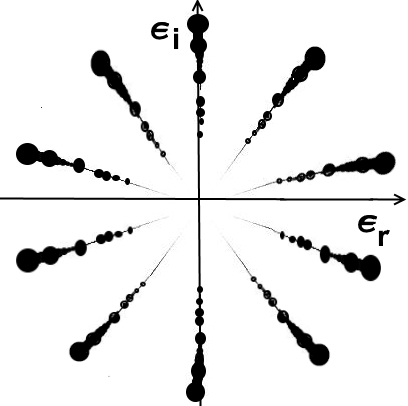
Figure 1. A representation of the set ${\mathcal{G}}$ given by the complement of the black circles, whose radii have been rescaled for graphical reasons. We took $d=1$, $\tau=1$, $a=5$.

References

- [Arn63] V. I. Arnol’d. Proof of a theorem of A. N. Kolmogorov on the invariance of quasi-periodic motions under small perturbations. Russian Math. Surveys, 18(5):9–36, 1963.
- [Arn64] V.I. Arnold. Instability of dynamical systems with several degrees of freedom. Sov. Math. Doklady, 5:581–585, 1964.
- [Ban02] A. Banyaga. Some properties of locally conformal symplectic structures. Comment. Math. Helv., 77(2):383–398, 2002.
- [BC18] A. P. Bustamante and R. Calleja. Computation of domains of analyticity for the dissipative standard map in the limit of small dissipation. Preprint, 2018.
- [BHS96] H. W. Broer, G. B. Huitema, and M. B. Sevryuk. Quasi-Periodic Motions in Families of Dynamical Systems. Order Amidst Chaos. Springer-Verlag, Berlin, 1996.
- [BHTB90] H. W. Broer, G. B. Huitema, F. Takens, and B. L. J. Braaksma. Unfoldings and bifurcations of quasi-periodic tori. Mem. Amer. Math. Soc., 83(421):viii+175, 1990.
- [CCCdlL17] Renato C. Calleja, Alessandra Celletti, Livia Corsi, and Rafael de la Llave. Response solutions for quasi-periodically forced, dissipative wave equations. SIAM J. Math. Anal., 49(4):3161–3207, 2017.
- [CCdlL13] Renato C. Calleja, Alessandra Celletti, and Rafael de la Llave. A KAM theory for conformally symplectic systems: efficient algorithms and their validation. J. Differential Equations, 255(5):978–1049, 2013.
- [CCdlL17] Renato C Calleja, Alessandra Celletti, and Rafael de la Llave. Domains of analyticity and Lindstedt expansions of KAM tori in some dissipative perturbations of Hamiltonian systems. Nonlinearity, 30(8):3151, 2017.
- [CCdlL18] Renato C. Calleja, Alessandra Celletti, and Rafael de la Llave. Existence of whiskered KAM tori of conformally symplectic systems. Preprint, https://arxiv.org/abs/1901.07483, 2019.
- [Cel10] Alessandra Celletti. Stability and Chaos in Celestial Mechanics. Springer-Verlag, Berlin; published in association with Praxis Publishing Ltd., Chichester, 2010.
- [CH17] Marta Canadell and Àlex Haro. Computation of quasiperiodic normally hyperbolic invariant tori: rigorous results. J. Nonlinear Sci., 27(6):1869–1904, 2017.
- [Cop78] W. A. Coppel. Dichotomies in stability theory. Lecture Notes in Mathematics, Vol. 629. Springer-Verlag, Berlin-New York, 1978.
- [DFIZ16a] Andrea Davini, Albert Fathi, Renato Iturriaga, and Maxime Zavidovique. Convergence of the solutions of the discounted equation: the discrete case. Math. Z., 284(3-4):1021–1034, 2016.
- [DFIZ16b] Andrea Davini, Albert Fathi, Renato Iturriaga, and Maxime Zavidovique. Convergence of the solutions of the discounted Hamilton-Jacobi equation: convergence of the discounted solutions. Invent. Math., 206(1):29–55, 2016.
- [dlL01] R. de la Llave. A tutorial on KAM theory. In Smooth ergodic theory and its applications (Seattle, WA, 1999), volume 69 of Proc. Sympos. Pure Math., pages 175–292. Amer. Math. Soc., Providence, RI, 2001.
- [dlLGJV05] R. de la Llave, A. González, À. Jorba, and J. Villanueva. KAM theory without action-angle variables. Nonlinearity, 18(2):855–895, 2005.
- [dlLS18] R. de la Llave and Y. Sire. An a posteriori KAM theorem for whiskered tori in Hamiltonian partial differential equations with applications to some ill-posed equations. Arch. Rational. Mech. Anal., https://doi.org/10.1007/s00205-018-1293-6, 2018.
- [DM96] C. P. Dettmann and G. P. Morriss. Proof of Lyapunov exponent pairing for systems at constant kinetic energy. Phys. Rev. E, 53(6):R5545–R5548, 1996.
- [FdlLS09] Ernest Fontich, Rafael de la Llave, and Yannick Sire. Construction of invariant whiskered tori by a parameterization method. Part I: maps and flows in finite dimensions. J. Differential Equations,, 246:3136–3213, 2009.
- [FdlLS15] Ernest Fontich, Rafael de la Llave, and Yannick Sire. Construction of invariant whiskered tori by a parameterization method. Part II: Quasi-periodic and almost periodic breathers in coupled map lattices. J. Differential Equations, 259(6):2180–2279, 2015.
- [HPS77] M.W. Hirsch, C.C. Pugh, and M. Shub. Invariant manifolds. Springer-Verlag, Berlin, 1977. Lecture Notes in Mathematics, Vol. 583.
- [LS15] Ugo Locatelli and Letizia Stefanelli. Quasi-periodic motions in a special class of dynamical equations with dissipative effects: a pair of detection methods. Discrete Contin. Dyn. Syst. Ser. B, 20(4):1155–1187, 2015.
- [Mos67] J. Moser. Convergent series expansions for quasi-periodic motions. Math. Ann., 169:136–176, 1967.
- [SL12] Letizia Stefanelli and Ugo Locatelli. Kolmogorov’s normal form for equations of motion with dissipative effects. Discrete Contin. Dynam. Systems, 17(7):2561–2593, 2012.
- [SS74] Robert J. Sacker and George R. Sell. Existence of dichotomies and invariant splittings for linear differential systems. I. J. Differential Equations, 15:429–458, 1974.
- [WL98] M. P. Wojtkowski and C. Liverani. Conformally symplectic dynamics and symmetry of the Lyapunov spectrum. Comm. Math. Phys., 194(1):47–60, 1998.