Dissipation of traffic congestion using agent-based car-following model with modified optimal velocity

Abstract

We investigate dynamical properties of traffic flow using the stochastic car-following model with modified optimal velocity on circular road. The safety distance following the two-second rule and autonomous vehicles, acting as agents, obeying simple requirements are incorporated into the model. The dynamic safety distance increases in a light traffic condition where the average driving velocity is high, while decreases in a dense traffic condition in anticipation of slower traffic motion. The results show that the presence of the agents can enhance overall velocity and traffic current of the system, and postpone the traffic congestion. In a particular phase region, imposing a speed limit enables the system to leave the congested flow phase. The density-dependent speed limit in agent-free condition is obtained to achieve the optimal traffic flow.

I Introduction

The collective motion of many-particle systems continues to be one of the most prominent topics studied in non-equilibrium processes Helbing (2001); Nagatani (2002); Chowdhury et al. (2005). Asymmetric interactions between particles are studied in transport systems because of their rich phenomena, such as phase transition, self-organization, and scaling behaviour Biham et al. (1992); Tajima and Nagatani (2001). Generally, mathematical modeling with regard to transport systems can be classified into one of the following three categories. i) Microscopic models are used to describe collective motion of individual particles that follow predefined transport rules. The cellular automata and car-following models are examples of this class of models Newell (1961); Kai Nagel and Michael Schreckenberg (1992). Others serve as pedagogical models that can be solved exactly for some processes, e.g., asymmetric simple exclusion process with open boundaries Derrida et al. (1992). ii) Mesoscopic models, also known as gas-kinetic models, are based on the Maxwell-Boltzmann transport theory of gases Prigogine and Andrews (1960). Lastly iii) macroscopic models where cars are coarse-grained and perceived as continuous fluid flow. Shock wave arising from discontinuity of the compressible fluid is viewed as traffic jam travelling backward with respect to the main flow Lighthill and Whitham (1955); Flynn et al. (2009). Micro-macroscopic links can be found following simple theoretical assumptions Lee et al. (2001). For many decades, the transport models have been successfully applied to many systems in seemingly different disciplines including ant movement John et al. (2009), pedestrian flow Helbing et al. (2000); Tajima and Nagatani (2001), and motions of molecular motors Klumpp and Lipowsky (2003).

In the area of vehicular transport, traffic congestion is one of the most pertinent issues that has been widely studied. Traffic signal optimization Arita et al. (2017), density and delay-feedback control Woelki (2013); Konishi et al. (2000), real-time information provision Yokoya (2004), and autonomous vehicles Stern et al. (2018) are examples of proposed methods to solve the problem. In this work, we use the stochastic car-following model with continuous spatial-temporal evolution to investigate the system on a circular road. According to the previous work, the safety distance in the optimal velocity function is independent of time and is the same for all drivers Nagatani (2002); Konishi et al. (2000); Bando et al. (1995a). However, the predefined safety distance is not practical for the drivers because it should depend on the average velocity of the car in the front. Normally, the advised safety distance for a driver follows what is known as the “two-second rule”. Our goal is to propose dynamic safety distance based on the two-second rule and autonomous driving agents to dissipate the traffic jam. The dynamic distance accounts for more realistic individual’s response that is not the same for every driver, is not fixed during the motion, and also depends on the driving velocity. As autonomous vehicles become gradually more available, they will increasingly play more central a role in reducing the traffic issues. The proposed agents, accounting for autonomous control units, require only basic information that is accessible with the current technology. We will show that the decrease in the traffic congestion can be achieved by increasing the number of such agents.

Our work is organized as follows. In Sec. II, the car-following model based on stochastic differential equations is presented. Modified optimal velocity, agents, model parameters, and computer simulation methods are described. Simulation results consisting of spatial-temporal traffic profiles, the average velocity as well as the traffic current, and the traffic phase diagram in steady states are shown in Sec. III. Finally, we discuss and conclude our work in Sec. IV.

II Car-Following Model

To simulate the dynamics of traffic phenomena, we adopt the stochastic car-following model with optimal velocity (OV) Bando et al. (1995b, a); Tadaki et al. (1998),

$$\mathrm{d}{X}_{i} = V_{i}\,\mathrm{d}{T},$$ (1)

$$\mathrm{d}{V}_{i} = \frac{1}{\tau}\left[V_{\text{opt}}\left(\Delta X_{i}\right)\mathrm{d}{T}-V_{i}\,\mathrm{d}{T}+\sqrt{2D}\,\mathrm{d}{W}_{i}\right],$$ (2)

where $X_{i}$ and $V_{i}$ are the position and velocity of car $i$, $\tau$ is the driver’s response time, $\Delta X_{i}=X_{i-1}-X_{i}$ is a headway distance of car $i$ measured from the center of car $i$ to the center of the preceding car $i-1$, $V_{\text{opt}}(\Delta X_{i})$ is an optimal velocity depending completely on the headway distance, $D$ is the diffusion constant relating to the strength of velocity variations, and the noise term $\mathrm{d}{W}_{i}\propto\sqrt{\mathrm{d}{T}}$ is a Wiener process. Each driver tries to adjust his or her velocity to reach the optimal velocity according to the headway distance. The change in the velocity is compensated by the response time and noise term characterizing individual’s behavior. Macroscopically, factor $\sqrt{D/\tau}$ is regarded as the velocity deviation or the velocity at which small perturbations of traffic flow travel Flynn et al. (2009). Let us introduce two system’s parameters: i) car’s length $X_{\text{car}}$ and ii) $V_{0}=X_{\text{car}}/\tau$, and define dimensionless parameters: $t=T/\tau$, $x_{i}=X_{i}/X_{\text{car}}$, $v_{i}=V_{i}/V_{0}$, $\sigma_{0}=(\sqrt{2D/\tau})/V_{0}$, and $\mathrm{d}{w}_{i}=\mathrm{d}{W}_{i}/\sqrt{\tau}$. Equations (1) and (2) become

$$\mathrm{d}{x}_{i} = v_{i}\mathrm{d}{t},$$ (3)

$$\mathrm{d}{v}_{i} = \left[v_{\text{opt}}\left(\Delta x_{i}\right)-v_{i}\right]\mathrm{d}{t}+\sigma_{0}\mathrm{d}{w}_{i}.$$ (4)

Eq. (4) is also known as Itô drift-diffusion process, where the first term on the right hand side is the drift term and the second term is the diffusion term. The optimal velocity is an increasing function of $\Delta x_{i}$ with conditions: (1) $v_{\text{opt}}\left(\Delta x_{i}\right)=u_{0}$ (the maximum velocity) when $\Delta x_{i}\rightarrow\infty$ and (2) $v_{\text{opt}}\left(\Delta x_{i}\right)=0$ when $\Delta x_{i}\leq\Delta x_{\text{min}}$ (some minimum distance). The first condition is to ensure the maximum velocity on an empty road, while the second condition is to avoid collision with other cars. A sigmoid function Bando et al. (1995b); Tadaki et al. (1998) is normally employed in this case:

$$v_{\text{opt}}\left(\Delta x_{i}\right)=u_{0}\left\{\frac{\tanh\left[a\left(\Delta x_{i}-\Delta x_{\text{safe}}-\Delta x_{\text{min}}\right)\right]+\tanh\left[a\left(\Delta x_{\text{safe}}\right)\right]}{1+\tanh\left[a\left(\Delta x_{\text{safe}}\right)\right]}\right\}$$ (5)

where safety distance $\Delta x_{\text{safe}}$ and $a$ are model parameters. Minimum distance $\Delta x_{\text{min}}$ is set to be $1$ (corresponding to the distance of one car), thus $\Delta x_{i}-\Delta x_{\text{min}}$ equals a distance from the front bumper of car $i$ to the rear bumper of car $i-1$.

II.1 Modified optimal velocity

In this work, safety distance $\Delta x_{\text{safe}}$ is replaced by a method of ensuring a safe headway, commonly known as the “two-second rule”

$$\Delta x_{\text{safe},i}=\bar{v}_{i-1}\Delta t_{\text{c}},$$ (6)

where $\Delta t_{\text{c}}=2~{}\text{seconds}/\tau$ is the recommended time for a driver to stay behind the car in the front to ensure that he or she receives enough time to respond and $\bar{v}_{i-1}$ is the temporal average velocity that the driver of car $i$ perceives of the preceding car. Note that we model the system on a circular road, so $\bar{v}_{N+1}=\bar{v}_{1}$. The remaining parameter to be specified is $a$. The sensitivity of the OV function with respect to small change $\Delta x_{i}$, i.e. $\mathrm{d}{v}_{\text{opt}}/\mathrm{d}{\Delta x_{i}}$, has the maximum value at $\Delta x_{i}=\Delta x_{\text{safe},i}+\Delta x_{\text{min}}$. We set the shape, or more precisely the full width at half maximum (FWHM), of the sensitivity to be scaled with its corresponding safety distance $\Delta x_{\text{safe},i}$. This means that optimal velocity ${v}_{\text{opt}}$ becomes less sensitive to headway distance $\Delta x_{i}$ when the safety distance increases. Parameter $a$ can then be determined from $\text{FWHM}=2\cosh^{-1}\left(\sqrt{2}\right)/a=\alpha\Delta x_{\text{safe},i}$, where $\alpha$ is a dimensionless scaling constant.

II.2 Agents

In this section, we introduce an autonomous car or an agent and implement a feasible method for agents to damp traffic congestion. An agent is a self-driving car equipped with a control unit. The Cognitive and Autonomous Test (CAT) vehicle Stern et al. (2018) is one example of such an agent. To differentiate agent with (normal) car driving behavior, a few simple rules are required for the agents. First, when a car in the front changes its velocity, the agent can react instantaneously and reaches its desired optimal velocity without any delay . Second, there are no fluctuations in the changing velocity, i.e. the noise term in Eq. (4) is zero. Small fluctuations resulting from human driving behavior are known to cause ‘stop-and-go’ wave to occur even from initially homogeneous motion Sugiyama et al. (2008); Stern et al. (2018). Finally, since autonomous driving is safer than manual driving, the agent can cruise at a shorter safety distance. Here we set $\Delta t_{\text{a}}$ to half that of the normal vehicles. For simplicity, the agents do not communicate with each other and have the same information as the normal drivers. There is no information, for example, about an incoming traffic wave, sharing among the agents.

II.3 Parameters and simulations

Here, we describe model parameters and simulation methods. We investigate the car-following model on a periodic road with the total distance of $l=100$ (equal to 100 cars). The normal car and agent densities are given by $\rho_{\text{c}}=n_{\text{c}}/l$ and $\rho_{\text{a}}=n_{\text{a}}/l$, where $n_{\text{c}}$ and $n_{\text{a}}$ are the numbers of normal cars and agents, respectively. The total number of vehicles on the road is $n=n_{\text{c}}+n_{\text{a}}\leq l$ corresponding to the total vehicle density of $\rho_{\text{t}}=n/l=\rho_{\text{c}}+\rho_{\text{a}}\leq 1$. Agents are placed randomly on the circular track. Imposed condition $\Delta x_{i}$ (or $\Delta x_{\text{safe},i}$) $=\Delta x_{\text{min}}$ is used whenever $\Delta x_{i}$ (or $\Delta x_{\text{safe},i}$) $<\Delta x_{\text{min}}$ so that $v_{\text{opt}}\left(\Delta x_{i}\right)=0$. The changes in velocity and position at time $t$ in Eqs. (3) and (4) are updated with fixed small time step $\mathrm{d}{t}=0.1$, corresponding to the physical time of about $50$ ms. At time $t^{\prime}=t+\mathrm{d}{t}$, velocity $v_{i}(t^{\prime})=v_{i}(t)+\mathrm{d}{v}_{i}(t)$ is modified for each vehicle within the range, $0\leq v_{i}(t^{\prime})\leq u_{0}$. Then spatial position $x_{i}(t^{\prime})=x_{i}(t)+\mathrm{d}{x}_{i}(t)$ is updated sequentially such that each car moves on the road without interfering with the car in the front.

The position and velocity of each car are tracked and measured. The average velocity at time $t$ is given by

$$v_{\text{av}}(t)=\frac{1}{n}\sum_{i=1}^{n}v_{i}(t).$$ (7)

We use the standard deviation $\sigma_{v}(t)$ of all car velocities to determine whether or not small initial perturbation $\sigma_{0}$ will be amplified during the motion. If $\sigma_{v}$ is greater than predetermined value, $\sigma_{\text{max}}=c\sigma_{0}$, the motion is considered to be congested. Constant $c=\sqrt{2}$ corresponds to $\sigma_{\text{max}}V_{0}=3.0~{}$m/s, which is close to the threshold of $2.5~{}$m/s used in the field experiments by Stern et al. Stern et al. (2018) to identify the onset of traffic wave. If congestion occurs, jamming state $J$ is said to be $1$, otherwise it is zero. Both $v_{\text{av}}$ and $J$ are averaged over the course of 1,000 and 500 trials, respectively. Finally if more than $50\%$ of the trials belong to state $J=1$, we justify the traffic condition to be in the congestion region. Some model constants are listed in Table 1.

Table 1: Constants used in this work.

parameter	value	units	Refs.
$\tau$	0.5	second (s)	Tadaki et al. (1998); Bando et al. (1995a)
$X_{\text{car}}$	5.0	meter (m)	Bando et al. (1995a)
$\sqrt{D/\tau}$	1.5	m/s
$\Delta x_{\text{min}}$	1.0	-
$\alpha$	0.5	-
$\Delta t_{\text{c}}$	4.0	-
$\Delta t_{\text{a}}$	2.0	-

III Simulation Results

III.1 Traffic profiles

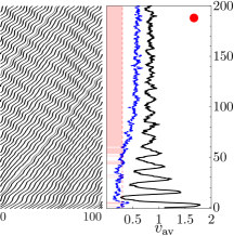
(a) $\rho_{\text{a}}=0.01$.

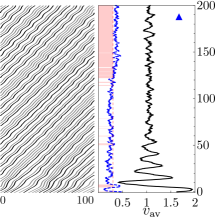
(b) $\rho_{\text{a}}=0.15$.

(c) $\rho_{\text{a}}=0.24$.

Figure 1: Trajectory profiles at total density $\rho_{\text{t}}=0.25$ with different agent densities: (a) $\rho_{\text{a}}=0.01$, (b) $\rho_{\text{a}}=0.15$, and (c) $\rho_{\text{a}}=0.24$. The normal car (agent) trajectory, moving from the left to the right, is indicated by the black (gray) line. Time direction increases from the bottom to the top. Corresponding average velocity $v_{\text{av}}$ (thick solid line) and standard deviation $\sigma_{v}$ (thick dashed line) are shown on the right hand side of each profile. Areas under the congestion threshold $\sigma_{\text{max}}$ (thin dashed line) are highlighted if $\sigma_{v}>\sigma_{\text{max}}$. The filled circle, up-triangle, and square symbols are used to mark traffic conditions of the profiles in different phase regions.

We first show simulation results with maximum velocity of $u_{0}=2.0$ (or about $72$ km/hr), unless otherwise stated. Fig. 1 shows three space-time profiles of car trajectories. The horizontal axis indicates car positions moving from left to right. The vertical axis shows the direction of time increasing from bottom to top. Each black (gray) line represents a car’s (an agent’s) trajectory. On the right hand side of each profile, average velocity $v_{\text{av}}$ (solid line) and standard deviation $\sigma_{v}$ (dashed line) are shown. The thin dashed line indicates congestion threshold $\sigma_{\text{max}}$. Highlighted areas denote when congestion occurs ($\sigma_{v}>\sigma_{\text{max}}$). The filled circle, up triangle, and square, shown at the upper right corner, represent particular conditions corresponding to the profiles that illustrate traffic motions in different phase regions which will be described in detail later in the next section. The total number of vehicles is kept at $\rho_{t}=0.25$. At the initial time, the car velocity is set closely to the optimal velocity.

The transient oscillations of $v_{\text{av}}$ are clearly seen before the traffic flow reaches non-equilibrium steady states. For $\rho_{\text{a}}\leq 0.15$ (Figs. 1(a) and (b)), initial noises are enhanced such that $\sigma_{v}$ exceeds threshold $\sigma_{\text{max}}$. At the steady state, the onset of permanent traffic congestion occurs. The characteristic shock wave traveling backward is clearly visible. For $\rho_{\text{a}}=0.24$ (Fig. 1(c)), on the other hand, initial perturbations are suppressed. Average velocity $v_{\text{av}}$ increases substantially at the steady state. For a small (large) number of agents, the traffic flow belongs to the jamming $J=1$ (free $J=0$) state. At a moderate agent density, e.g. $\rho_{\text{a}}=0.15$ the flow lies close to the boundary region with state $J$ being either $0$ or $1$. Compared to the results where the agents are absent, $v_{\text{av}}$ increases by 2%, 26%, and 57% for $\rho_{\text{a}}=0.01$, $0.15$, and $0.24$, respectively. It is noted that for $\rho_{\text{a}}=0.24$ even a few drivers may reduce the traffic flow overall.

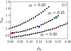
Figure 2: (a) Average velocity $v_{\text{av}}$ versus total density $\rho_{\text{t}}$ for $\rho_{\text{a}}=0$ (empty and filled circles) and $\rho_{\text{c}}=0$ (filled diamonds). The empty circle data corresponds to OV with fixed $\Delta x_{\text{safe},i}=20~{}\text{meters}/X_{\text{car}}=4$. (b) The traffic current, $q=\rho v_{\text{av}}$, versus car density $\rho_{\text{c}}$ of those results with $\rho_{\text{a}}=0$ in Fig. 2(a). (c) Average velocity $v_{\text{av}}$ versus agent density $\rho_{\text{a}}$ for $\rho_{\text{t}}=0.20$, $0.25$, and $0.30$. The filled circle, up-triangle, and square symbols at $\rho_{\text{t}}=0.25$ correspond to the profiles in Fig. 1.

To study the traffic flow at the steady states, velocities of individual vehicles are averaged after simulation time $t=50$ for various values of traffic density. Fig. 2(a) shows $v_{\text{av}}$ versus $\rho_{\text{t}}$ plot of the limiting cases where only normal drivers are present on the road, i.e., $\rho_{\text{a}}=0$ (empty and filled circles) with total density $\rho_{\text{t}}$ being $\rho_{\text{t}}=\rho_{\text{c}}$ and only agents on the road, $\rho_{\text{c}}=0$ (filled diamonds) with $\rho_{\text{t}}=\rho_{\text{a}}$. For the former case with $\rho_{\text{a}}=0$, filled circles are the simulation results with modified OV, while empty circles are those with static safety distance $\Delta x_{\text{safe},i}$ being set to 4.0 corresponding to physical safety distance of 20 meters Bando et al. (1995a). With modified OV, the average velocity is maintained at $v_{\text{av}}\simeq 1.9$ up to $\rho_{\text{t}}$ of about $8\%$ before $v_{\text{av}}$ drops continuously at a higher density. It is noted that at the low traffic region, each driver does not always cruise at the maximum velocity of $u_{0}=2.0$ because of small fluctuations introduced in the system, thus $v_{\text{av}}<u_{0}$. Although $v_{\text{av}}$ decreases sooner than that with fixed $\Delta x_{\text{safe},i}$, the rate at which it decreases is lower.

Average velocity $v_{\text{av}}$ reaches the maximum velocity $u_{0}$ when there are only agents on the road in the low traffic region due to the absence of noises in the system. The average velocity then slowly decreases at a higher car density to compensate for the smaller headway distance. The traffic flow is improved for all traffic conditions, particularly in the heavy traffic. Compared with the results without any agents ($\rho_{\text{a}}=0$), systems with agents show moderate (5% increase in average speed at $\rho_{\text{t}}=0.01$, for example) to remarkable speed boost (64% increase at $\rho_{\text{t}}=0.22$). The results suggest the obvious benefits of the agents in diminishing the traffic congestion.

Fig. 2(b) shows traffic current $q\equiv\rho v_{\text{av}}$ of the results with the absence of agents. For OV with static $\Delta x_{\text{safe},i}=4$ (empty circle data), the sharp change with a possible discontinuity Bando et al. (1995a) connecting free flow and congested flow phases is visible. Current $q$ in the heavy traffic is not zero and is again due to the effect of the diffusion term. Although the modified OV model with the two-second rule (filled circle data) does not improve the traffic current much at low $\rho_{\text{c}}$; it is even worse at the boundary, the model enhances the traffic current considerably when the traffic becomes congested at high $\rho_{\text{c}}$. Note that a sharp change in $q$ is not visible in this result.

Traffic flow can be improved further by turning the cars to the agents as illustrated in Fig. 2(c). The trend is similar for all conditions of total density $\rho_{\text{t}}$. For each line, the result is bounded between its minimum at $\rho_{\text{a}}=0$ and its maximum at $\rho_{\text{c}}=0$ as shown in Fig. 2(a) for a given $\rho_{\text{t}}$. The symbols: filled circle, up-triangle, and square represent those conditions whose traffic profiles are shown in Fig. 1.

III.2 Phase diagram

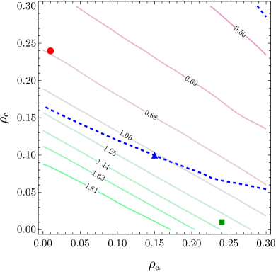
Figure 3: Contour plot of $v_{\text{av}}$ as a function of normal car density $\rho_{\text{c}}$ and agent density $\rho_{\text{a}}$ with limit velocity $u_{0}=$ 2.0. The dashed line indicates a traffic congestion boundary between free flow and congested flow. The filled squares and circles are some of those conditions belonging to free flow and congested flow, while the filled triangle indicates a condition lying close to the boundary.

We turn our attention to a phase diagram between the free flow and congested flow phases. Fig. 3 shows a contour plot of average velocity $v_{\text{av}}$ versus normal car density $\rho_{\text{c}}$ and agent density $\rho_{\text{a}}$. As described earlier, $v_{\text{av}}$ is improved considerably when all cars are agents for a given total density $\rho_{\text{t}}$. The information of $v_{\text{av}}$ alone, however, does not completely specified the traffic situation. Smooth and stable motion relating to fuel consumption, braking event, and car collision are also important parameters of interest, which are hinted by the traffic phase diagram.

If more than half of the trials belong to jamming state $J=1$, the traffic condition more likely leads to a congestion. We therefore categorize this condition as belonging to the congested flow phase, otherwise it is in the free flow phase. The boundary separating these two phases are indicated by the dashed line in Fig. 3. It is obvious that the traffic phase depends strongly on the number of normal cars on the tracks. At $\rho_{\text{c}}=0.05$, for example, the traffic is in the free flow phase, regardless of the number of agents. Moreover, for a given total density $\rho_{\text{t}}$ (e.g. $\rho_{\text{t}}=0.25$), increasing the number of agents will postpone the traffic jam—from congested flow (filled circle data) to the boundary (filled triangle data), and to the free flow (filled square data). It should be noted that at high density, e.g., $\rho_{\text{t}}=0.6$, the system belongs to the free flow phase. This is because short wavelength perturbations are suppressed by the narrow headway distance such that very little velocity variation takes place ($\sigma_{v}$ does not exceed the congestion threshold). Even though the traffic is not congested, the average velocity in the region is not very high. This suggests that $v_{\text{av}}$ and traffic phase should be considered together if we want to limit the number of normal cars or to increase the number of agents before the traffic enters the congested flow phase.

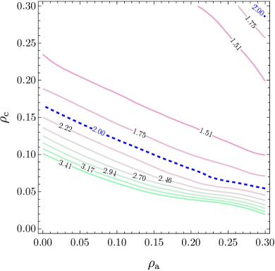
Figure 4: Maximum velocity $u_{0}$ in a free flow phase as functions of normal car density $\rho_{\text{c}}$ and agent density $\rho_{\text{a}}$. The dashed line represents the maximum velocity of $u_{0}=2.0$.

In practice, restricting the number of cars and/or agents is often not practical. It is however still possible to regulate the free flow by limiting speed limit $u_{0}$. A natural question arises: given a traffic condition, what is the speed limit beyond which the traffic becomes congested? Fig. 4 shows the contour plot of the speed limit versus normal car density $\rho_{\text{c}}$ and agent density $\rho_{\text{a}}$ in the free flow phase. The dashed line marks the maximum velocity of $u_{0}=2.0$. Below the dashed line is an area that $u_{0}$ can be set higher than $u_{0}=2.0$. At $\rho_{\text{a}}=0.30$ with a few normal cars, for example, the maximum velocity can be up to $u_{0}=3.41$ corresponding to the physical velocity of about $120$ km/hr, which exceeds the speed limit allowed in many countries. Above the dashed line is the area where we have to lower the speed limit.

Figure 5: Maximum velocity $u_{0}$ in a free flow phase with $\rho_{a}=0$ versus normal car density $\rho_{c}$.

Fig. 5 shows, for instant, variable speed limit as a function of car density in the absence of agents. As expected, the limit decreases continuously as the car density increases. The result can be adapted directly as a new traffic control strategy.

IV Discussion and Conclusion

We study the dynamics of the stochastic car-following model with the optimal velocity function on a circular road. Two strategies are employed in this work. First, we incorporate the two-second rule to determine the safety distance to ensure a more realistic driver’s response. When we apply the rule to the normal drivers (see Fig. 2(a) for $\rho_{\text{a}}=0$), average velocity $v_{\text{av}}$ is less than that of the OV with fixed $\Delta x_{\text{safe},i}=4.0$ in light traffic condition, while it becomes greater at a particular traffic density. The crossover of the behavior is due to the fact that at low $\rho_{\text{t}}$, a driver following the two-second rule tends to leave a wider safety distance, hence slower optimal velocity. At a crossover $\rho_{\text{t}}$ where the traffic becomes heavier, each driver lowers his or her safety distance to compensate for the flow such that all cars can continue to move collectively on the crowded road. We intend to modify the optimal velocity in this way because when there are several cars on the road, it is generally not safe to drive the car at high speed while keeping the safety distance too small. At dense traffic, in contrast, it is not necessary to leave a wide safety distance because of the slow, congested traffic. In fact, the cars are nearly bumper-to-bumper. It turns out that the modification of the safety distance improves the traffic condition noticeably in a heavy traffic condition.

Second, we add to the model autonomous vehicles, acting as agents, with a few simple rules. As expected, agents increase the average velocity of the system for all traffic conditions. The presence of the agents not only reduces fluctuations in the system but also provides more available road space since the agents cruise at a shorter safety distance. Moreover, if the headway distance is large enough that it looks as if the cars move on the road with low density traffic, uniform motion will be stable against small fluctuations. Under such conditions, agents can definitely dissipate the traffic congestion and increase overall traffic current, particularly in the heavy traffic region as suggested by the results in Fig. 2(a). The strategies show promising results, which may additionally save more fuel consumption, reduce braking events, and car collisions due to the uniform motion of the vehicles Stern et al. (2018).

To promote the traffic flow with normal cars and agents all together, there are two possible solutions. The first one is to restrict the number of normal cars or increase the number of agents to postpone the traffic jam (see Fig. 3). We note that maximizing either average velocity or traffic current alone is not adequate, since the traffic may encounter the congested state according to the results in Fig. 2(b). The other one is to adjust the maximum velocity for a given traffic density such that the traffic is still in the free flow phase. The imposing limit is suggested by the results in Fig. 4. The latter strategy can be implemented immediately in practice, given the ubiquity of traffic cameras from which the car density can be calculated.