Continuous Hierarchical Representations with
Poincaré Variational Auto-Encoders

Abstract

The variational auto-encoder (vae) is a popular method for learning a generative model and embeddings of the data. Many real datasets are hierarchically structured. However, traditional vaes map data in a Euclidean latent space which cannot efficiently embed tree-like structures. Hyperbolic spaces with negative curvature can. We therefore endow vaes with a Poincaré ball model of hyperbolic geometry as a latent space and rigorously derive the necessary methods to work with two main Gaussian generalisations on that space. We empirically show better generalisation to unseen data than the Euclidean counterpart, and can qualitatively and quantitatively better recover hierarchical structures.

1 Introduction

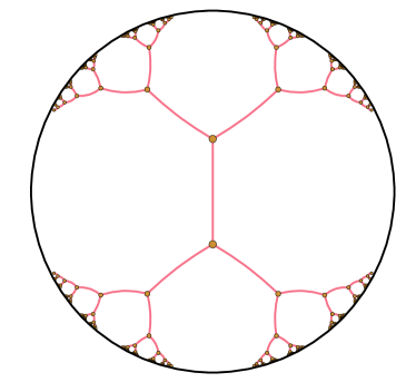
Figure 1: A regular tree isometrically embedded in the Poincaré disc. Red curves are same length geodesics, i.e. "straight lines".

Learning useful representations from unlabelled raw sensory observations, which are often high-dimensional, is a problem of significant importance in machine learning. Variational auto-encoders (vaes)(Kingma and Welling,, 2014; Rezende et al.,, 2014) are a popular approach to this: they are probabilistic generative models composed of an encoder stochastically embedding observations in a low dimensional latent space $\mathcal{Z}$, and a decoder generating observations $\bm{x}\in\mathcal{X}$ from encodings $\bm{z}\in\mathcal{Z}$. After training, the encodings constitute a low-dimensional representation of the original raw observations, which can be used as features for a downstream task (e.g. Huang and LeCun,, 2006; Coates et al.,, 2011) or be interpretable for their own sake. Vaes are therefore of interest for representation learning (Bengio et al.,, 2013), a field which aims to learn good representations, e.g. interpretable representations, ones yielding better generalisation, or ones useful for downstream tasks.

It can be argued that in many domains data should be represented hierarchically. For example, in cognitive science, it is widely accepted that human beings use a hierarchy to organise object categories (e.g. Roy et al.,, 2006; Collins and Quillian,, 1969; Keil,, 1979). In biology, the theory of evolution (Darwin,, 1859) implies that features of living organisms are related in a hierarchical manner given by the evolutionary tree. Explicitly incorporating hierarchical structure in probabilistic models has unsurprisingly been a long-running research topic (e.g. Duda et al.,, 2000; Heller and Ghahramani,, 2005).

Earlier work in this direction tended to use trees as data structures to represent hierarchies. Recently, hyperbolic spaces have been proposed as an alternative continuous approach to learn hierarchical representations from textual and graph-structured data (Nickel and Kiela,, 2017; Tifrea et al.,, 2019). Hyperbolic spaces can be thought of as continuous versions of trees, and vice versa, as illustrated in Figure 1. Trees can be embedded with arbitrarily low error into the Poincaré disc model of hyperbolic geometry (Sarkar,, 2012). The exponential growth of the Poincaré surface area with respect to its radius is analogous to the exponential growth of the number of leaves in a tree with respect to its depth. Further, these spaces are smooth, enabling the use of deep learning approaches which rely on differentiability.

We show that replacing vaes latent space components, which traditionally assume a Euclidean metric over the latent space, by their hyperbolic generalisation helps to represent and discover hierarchies. Our goals are twofold: (a) learn a latent representation that is interpretable in terms of hierarchical relationships among the observations, (b) learn a more efficient representation which generalises better to unseen data that is hierarchically structured. Our main contributions are as follows:

1. We propose efficient and reparametrisable sampling schemes, and calculate the probability density functions, for two canonical Gaussian generalisations defined on the Poincaré ball, namely the maximum-entropy and wrapped normal distributions. These are the ingredients required to train our vaes.

2. We introduce a decoder architecture that explicitly takes into account the hyperbolic geometry, which we empirically show to be crucial.

3. We empirically demonstrate that endowing a vae with a Poincaré ball latent space can be beneficial in terms of model generalisation and can yield more interpretable representations.

Our work fits well with a surge of interest in combining hyperbolic geometry and vaes. Of these, it relates most strongly to the concurrent works of Ovinnikov, (2018); Grattarola et al., (2019); Nagano et al., (2019). In contrast to these approaches, we introduce a decoder that takes into account the geometry of the hyperbolic latent space. Along with the wrapped normal generalisation used in the latter two articles, we give a thorough treatment of the maximum entropy normal generalisation and a rigorous analysis of the difference between the two. Additionally, we train our model by maximising a lower bound on the marginal likelihood, as opposed to Ovinnikov, (2018); Grattarola et al., (2019) which consider a Wasserstein and an adversarial auto-encoder setting, respectively. We discuss these works in more detail in Section 4.

2 The Poincaré Ball model of hyperbolic geometry

2.1 Review of Riemannian geometry

Throughout the paper we denote the Euclidean norm and inner product by $\left\|\cdot\right\|$ and $\langle\cdot,\cdot\rangle$ respectively. A real, smooth manifold $\mathcal{M}$ is a set of points $\bm{z}$, which is "locally similar" to a linear space. For every point $\bm{z}$ of the manifold $\mathcal{M}$ is attached a real vector space of the same dimensionality as $\mathcal{M}$ called the tangent space $\mathcal{T}_{\bm{z}}\mathcal{M}$. Intuitively, it contains all the possible directions in which one can tangentially pass through $\bm{z}$. For each point $\bm{z}$ of the manifold, the metric tensor $\mathfrak{g}(\bm{z})$ defines an inner product on the associated tangent space : $\mathfrak{g}(\bm{z})=\langle\cdot,\cdot\rangle_{\bm{z}}:\mathcal{T}_{\bm{z}}\mathcal{M}\times\mathcal{T}_{\bm{z}}\mathcal{M}\rightarrow\mathbb{R}$. The matrix representation of the Riemannian metric $G(\bm{z})$, is defined such that $\forall\bm{u},\bm{v}\in\mathcal{T}_{\bm{z}}\mathcal{M}\times\mathcal{T}_{\bm{z}}\mathcal{M},\ \langle\bm{u},\bm{v}\rangle_{\bm{z}}=\mathfrak{g}(\bm{z})(\bm{u},\bm{v})=\bm{u}^{T}G(\bm{z})\bm{v}$. A Riemannian manifold is then defined as a tuple $(\mathcal{M},\mathfrak{g})$ (Petersen,, 2006). The metric tensor gives a local notion of angle, length of curves, surface area and volume, from which global quantities can be derived by integrating local contributions. A norm is induced by the inner product on $\mathcal{T}_{\bm{z}}\mathcal{M}$: $\left\|\cdot\right\|_{\bm{z}}=\sqrt{\langle\cdot,\cdot\rangle_{\bm{z}}}$. An infinitesimal volume element is induced on each tangent space $\mathcal{T}_{\bm{z}}\mathcal{M}$, and thus a measure $d\mathcal{M}(\bm{z})=\sqrt{|G(\bm{z})|}d\bm{z}$ on the manifold, with $d\bm{z}$ being the Lebesgue measure. The length of a curve $\gamma:t\mapsto\gamma(t)\in\mathcal{M}$ is given by $L(\gamma)=\int_{0}^{1}{\|\gamma^{\prime}(t)\|_{\gamma(t)}^{1/2}dt}$. The concept of straight lines can then be generalised to geodesics, which are constant speed curves giving the shortest path between pairs of points $\bm{z},\bm{y}$ of the manifold: $\gamma^{*}=\operatorname*{arg\,min}L(\gamma)$ with $\gamma(0)=\bm{z}$, $\gamma(1)=\bm{y}$ and $\left\|\gamma^{\prime}(t)\right\|_{\gamma(t)}=1$. A global distance is thus induced on $\mathcal{M}$ given by $d_{\mathcal{M}}(\bm{z},\bm{y})=\inf L(\gamma)$. Endowing $\mathcal{M}$ with that distance consequently defines a metric space $(\mathcal{M},d_{\mathcal{M}})$. The concept of moving along a "straight" curve with constant velocity is given by the exponential map. In particular, there is a unique unit speed geodesic $\gamma$ satisfying $\gamma(0)=\bm{z}$ with initial tangent vector $\gamma^{\prime}(0)=\bm{v}$. The corresponding exponential map is then defined by $\exp_{\bm{z}}(\bm{v})=\gamma(1)$, as illustrated on Figure 2. The logarithm map is the inverse $\log_{\bm{z}}=\exp_{\bm{z}}^{-1}:\mathcal{M}\rightarrow\mathcal{T}_{\bm{z}}\mathcal{M}$. For geodesically complete manifolds, such as the Poincaré ball, $\exp_{\bm{z}}$ is well-defined on the full tangent space $\mathcal{T}_{\bm{z}}\mathcal{M}$ for all $z\in\mathcal{M}$.

2.2 The Poincaré ball model of hyperbolic geometry

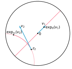
Figure 2: Geodesics and exponential maps in the Poincaré disc.

A $d$-dimensional hyperbolic space, denoted $\mathbb{H}^{d}$, is a complete, simply connected, $d$-dimensional Riemannian manifold with constant negative curvature $c$. In contrast with the Euclidean space $\mathbb{R}^{d}$, $\mathbb{H}^{d}$ can be constructed using various isomorphic models (none of which is prevalent), including the hyperboloid model, the Beltrami-Klein model, the Poincaré half-plane model and the Poincaré ball $\mathcal{B}_{c}^{d}$ (Beltrami,, 1868). The Poincaré ball model is formally defined as the Riemannian manifold $\mathbb{B}_{c}^{d}=(\mathcal{B}_{c}^{d},\mathfrak{g}_{p}^{c})$, where $\mathcal{B}_{c}^{d}$ is the open ball of radius $1/\sqrt{c}$, and $\mathfrak{g}_{p}^{c}$ its metric tensor, which along with its induced distance are given by

$$\mathfrak{g}_{p}^{c}(\bm{z})=({\lambda_{\bm{z}}^{c})}^{2}~{}\mathfrak{g}_{e}(\bm{z}),\ \ d^{c}_{p}(\bm{z},\bm{y})=\frac{1}{\sqrt{c}}\cosh^{-1}\left(1+2c\frac{||\bm{z}-\bm{y}||^{2}}{(1-c\left\|\bm{z}\right\|^{2})(1-c\left\|\bm{y}\right\|^{2})}\right),$$

where $\lambda_{\bm{z}}^{c}=\frac{2}{1-c\left\|\bm{z}\right\|^{2}}$ and $\mathfrak{g}_{e}$ denotes the Euclidean metric tensor, i.e. the usual dot product.

The Möbius addition (Ungar,, 2008) of $\bm{z}$ and $\bm{y}$ in $\mathbb{B}^{d}_{c}$ is defined as

$$\bm{z}\oplus_{c}\bm{y}=\frac{(1+2c\left\langle\bm{z},\bm{y}\right\rangle+c\|\bm{y}\|^{2})\bm{z}+(1-c\|\bm{z}\|^{2})\bm{y}}{1+2c\left\langle\bm{z},\bm{y}\right\rangle+c^{2}\|\bm{z}\|^{2}\|\bm{y}\|^{2}}.$$

One recovers the Euclidean addition of two vectors in $\mathbb{R}^{d}$ as $c\rightarrow 0$. Building on that framework, Ganea et al., (2018) derived closed-form formulations for the exponential map (illustrated in Figure 2)

$$\exp^{c}_{\bm{z}}(\bm{v})=\bm{z}\oplus_{c}\left(\tanh\left(\sqrt{c}\frac{\lambda^{c}_{\bm{z}}\|\bm{v}\|}{2}\right)\frac{\bm{v}}{\sqrt{c}\|\bm{v}\|}\right)$$

and its inverse, the logarithm map

$$\log^{c}_{\bm{z}}(\bm{y})=\frac{2}{\sqrt{c}\lambda^{c}_{\bm{z}}}\tanh^{-1}\left(\sqrt{c}\|-\bm{z}\oplus_{c}\bm{y}\|\right)\frac{-\bm{z}\oplus_{c}\bm{y}}{\|-\bm{z}\oplus_{c}\bm{y}\|}.$$

3 The Poincaré VAE

We consider the problem of mapping an empirical distribution of observations to a lower dimensional Poincaré ball $\mathbb{B}_{c}^{d}$, as well as learning a map from this latent space $\mathcal{Z}=\mathbb{B}_{c}^{d}$ to the observation space $\mathcal{X}$. Building on the vae framework, this Poincaré-vae model, or $\mathcal{P}^{c}$-VAE for short, differs by the choice of prior and posterior distributions being defined on $\mathbb{B}_{c}^{d}$, and by the encoder $g_{\bm{\phi}}$ and decoder $f_{\bm{\theta}}$ maps which take into account the latent space geometry. Their parameters $\{\bm{\theta},\bm{\phi}\}$ are learned by maximising the evidence lower bound (elbo). Our model can be seen as a generalisation of a classical Euclidean vae (Kingma and Welling,, 2014; Rezende et al.,, 2014) that we denote by $\mathcal{N}$-VAE, i.e. $\mathcal{P}^{c}$-VAE $\xrightarrow[c\rightarrow 0]{}\mathcal{N}$-VAE.

3.1 Prior and variational posterior distributions

In order to parametrise distributions on the Poincaré ball, we consider two canonical generalisations of normal distributions on that space. A more detailed review of Gaussian generalisations on manifolds can be found in Appendix B.1.

Riemannian normal

One generalisation is the distribution maximising entropy given an expectation and variance (Said et al.,, 2014; Pennec,, 2006; Hauberg,, 2018), often called the Riemannian normal distribution, which has a density w.r.t. the metric induced measure $d\mathcal{M}$ given by

$$\mathcal{N}^{\text{R}}_{\mathbb{B}_{c}^{d}}(\bm{z}|\bm{\mu},\sigma^{2})=\frac{d\nu^{\text{R}}(\bm{z}|\bm{\mu},\sigma^{2})}{d\mathcal{M}(\bm{z})}=\frac{1}{Z^{\text{R}}}\exp\left(-\frac{d_{p}^{c}(\bm{\mu},\bm{z})^{2}}{2\sigma^{2}}\right),$$ (1)

where $\sigma>0$ is a dispersion parameter, $\bm{\mu}\in\mathbb{B}_{c}^{d}$ is the Fréchet mean , and $Z^{\text{R}}$ is the normalising constant derived in Appendix B.4.3.

Figure 3: Hyperbolic normal probability density for different Fréchet mean, same standard deviation and $c=10$. The Riemannian hyperbolic radius has a slightly larger mode.

Wrapped normal

An alternative is to consider the pushforward measure obtained by mapping a normal distribution along the exponential map $\exp_{\bm{\mu}}$. That probability measure is often referred to as the wrapped normal distribution, and has been used in auto-encoder frameworks with other manifolds (Grattarola et al.,, 2019; Nagano et al.,, 2019; Falorsi et al.,, 2018). Samples $\bm{z}\in\mathbb{B}_{c}^{d}$ are obtained as $\bm{z}=\exp^{c}_{\bm{\mu}}\left({\bm{\bm{v}}}/{\lambda^{c}_{\bm{\mu}}}\right)$ with $\bm{\bm{v}}\sim\mathcal{N}(\cdot|\bm{0},\Sigma)$ and its density is given by (details given in Appendix B.3)

$$\mathcal{N}^{\text{W}}_{\mathbb{B}_{c}^{d}}(\bm{z}|\bm{\mu},\Sigma)=\frac{d\nu^{\text{W}}(\bm{z}|\bm{\mu},\Sigma)}{d\mathcal{M}(\bm{z})}$$ (2)

$$=\mathcal{N}\left(\lambda^{c}_{\bm{\mu}}\log_{\bm{\mu}}(\bm{z})\middle|\bm{0},\Sigma\right)\left(\frac{\sqrt{c}~{}d_{p}^{c}(\bm{\mu},\bm{z})}{\sinh(\sqrt{c}~{}d_{p}^{c}(\bm{\mu},\bm{z}))}\right)^{d-1}.$$

The (usual) normal distribution is recovered for both generalisations as $c\rightarrow 0$. We discuss the benefits and drawbacks of those two distributions in Appendix B.1. We refer to both as hyperbolic normal distributions with pdf $\mathcal{N}_{\mathbb{B}_{c}^{d}}(\bm{z}|\bm{\mu},\sigma^{2})$. Figure 8 shows several probability densities for both distributions.

The prior distribution defined on $\mathcal{Z}$ is chosen to be a hyperbolic normal distribution with mean zero, $p(\bm{z})=\mathcal{N}_{\mathbb{B}^{d}_{c}}(\cdot|\bm{0},\sigma_{0}^{2})$, and the variational family is chosen to be parametrised as $\mathcal{Q}=\{\mathcal{N}_{\mathbb{B}_{c}^{d}}(\cdot|\bm{\mu},\sigma^{2})~{}|~{}\bm{\mu}\in\mathbb{B}_{c}^{d},\sigma\in\mathbb{R}^{+}_{*}\}$.

3.2 Encoder and decoder

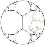
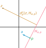
Figure 4: Illustration of an orthogonal projection on a hyperplane in a Poincaré disc (Left) and an Euclidean plane (Right).

We make use of two neural networks, a decoder $f_{\bm{\theta}}$ and an encoder $g_{\bm{\phi}}$, to parametrise the likelihood $p(\cdot|f_{\bm{\theta}}(\bm{z}))$ and the variational posterior $q(\cdot|g_{\bm{\phi}}(\bm{x}))$ respectively. The input of $f_{\bm{\theta}}$ and the output of $g_{\bm{\phi}}$ need to respect the hyperbolic geometry of $\mathcal{Z}$. In the following we describe appropriate choices for the first layer of the decoder and the last layer of the encoder.

Decoder

In the Euclidean case, an affine transformation can be written in the form $f_{\bm{a},\bm{p}}(\bm{z})=\left\langle\bm{a},\bm{z}-\bm{p}\right\rangle$, with orientation and offset parameters $\bm{a},\bm{p}\in\mathbb{R}^{d}$. This can be rewritten in the form

$$f_{\bm{a},\bm{p}}(\bm{z})=\text{sign}(\left\langle\bm{a},\bm{z}-\bm{p}\right\rangle)\left\|\bm{a}\right\|d_{E}(\bm{z},H^{c}_{\bm{a},\bm{p}})$$

where $H_{\bm{a},\bm{p}}=\{\bm{z}\in\mathbb{R}^{p}~{}|~{}\left\langle\bm{a},\bm{z}-\bm{p}\right\rangle=0\}=\bm{p}+\{\bm{a}\}^{\perp}$ is the decision hyperplane. The third term is the distance between $\bm{z}$ and the decision hyperplane $H^{c}_{\bm{a},\bm{p}}$ and the first term refers to the side of $H^{c}_{\bm{a},\bm{p}}$ where $\bm{z}$ lies. Ganea et al., (2018) analogously introduced an operator $f^{c}_{\bm{a},\bm{p}}:\mathbb{B}_{c}^{d}\rightarrow\mathbb{R}^{p}$ on the Poincaré ball,

$$f^{c}_{\bm{a},\bm{p}}(\bm{z})=\text{sign}(\left\langle\bm{a},\log^{c}_{\bm{p}}(\bm{z})\right\rangle_{\bm{p}})\left\|\bm{a}\right\|_{\bm{p}}d^{c}_{p}(\bm{z},H^{c}_{\bm{a},\bm{p}})$$

with $H^{c}_{\bm{a},\bm{p}}=\{\bm{z}\in\mathbb{B}_{c}^{d}~{}|~{}\left\langle\bm{a},\log^{c}_{\bm{p}}(\bm{z})\right\rangle=0\}=\exp^{c}_{\bm{p}}(\{\bm{a}\}^{\perp})$. A closed-formed expression for the distance $d^{c}_{p}(\bm{z},H^{c}_{\bm{a},\bm{p}})$ was also derived, $d^{c}_{p}(\bm{z},H^{c}_{\bm{a},\bm{p}})=\frac{1}{\sqrt{c}}\sinh^{-1}\left(\frac{2\sqrt{c}|\left\langle-\bm{p}\oplus_{c}\bm{z},a\right\rangle|}{(1-c\|-\bm{p}\oplus_{c}\bm{z}\|^{2})\|\bm{a}\|}\right)$. The hyperplane decision boundary $H^{c}_{\bm{a},\bm{p}}$ is called gyroplane and is a semi-hypersphere orthogonal to the Poincaré ball’s boundary as illustrated on Figure 4. The decoder’s first layer, called gyroplane layer, is chosen to be a concatenation of such operators, which are then composed with a standard feed-forward neural network.

Encoder

The encoder $g_{\bm{\phi}}$ outputs a Fréchet mean $\bm{\mu}\in\mathbb{B}_{c}^{d}$ and a distortion $\sigma\in\mathbb{R}^{+}_{*}$ which parametrise the hyperbolic variational posterior. The Fréchet mean $\bm{\mu}$ is obtained as the image of the exponential map $\exp^{c}_{\bm{0}}$, and the distortion $\sigma$ through a softplus function.

3.3 Training

We follow a standard variational approach by deriving a lower bound on the marginal likelihood. The elbo is optimised via an unbiased Monte Carlo (mc) estimator thanks to the reparametrisable sampling schemes that we introduce for both hyperbolic normal distributions.

Objective

The evidence lower bound (elbo)can readily be extended to Riemannian latent spaces by applying Jensen’s inequality w.r.t. $d\mathcal{M}$ (see Appendix A)

$$\log p(\bm{x})\geq\mathcal{L}_{\mathcal{M}}(\bm{x};\theta,\phi)\triangleq\int_{\mathcal{M}}\ln\left(\frac{p_{\theta}(\bm{x}|\bm{z})p(\bm{z})}{q_{\phi}(\bm{z}|\bm{x})}\right)\ q_{\phi}(\bm{z}|\bm{x})\ d\mathcal{M}(\bm{z}).$$

Densities have been introduced earlier in Equations 1 and 2.

Reparametrisation

Algorithm 1 Hyperbolic normal sampling scheme

$\bm{\mu}$, $\sigma^{2}$, dimension $d$, curvature $c$

if Wrapped normal then $\bm{v}\sim\mathcal{N}(\bm{0}_{d},\sigma^{2})$

else if Riemannian normal then

     Let $g$ be a piecewise exponential proposal

     while sample $r$ not accepted do

         Propose $r\sim g(\cdot)$, $u\sim\mathcal{U}([0,1])$

         if $u<\frac{\rho^{\text{R}}(r)}{g(r)}$ then Accept sample $r$               

     Sample direction $\bm{\alpha}\sim\mathcal{U}(\mathbb{S}^{d-1})$

     $\bm{v}\leftarrow r\bm{\alpha}$

Return $\bm{z}=\exp^{c}_{\bm{\mu}}\left({\bm{v}}/{\lambda^{c}_{\bm{\mu}}}\right)$

In the Euclidean setting, by working in polar coordinates, an isotropic normal distribution centred at $\bm{\mu}$ can be described by a directional vector $\bm{\alpha}$ uniformly distributed on the hypersphere and a univariate radius $r=d_{E}(\bm{\mu},\bm{z})$ following a ${\chi}$-distribution. In the Poincaré ball we can rely on a similar representation, through a hyperbolic polar change of coordinates, given by

$$\bm{z}=\exp^{c}_{\bm{\mu}}\left(G(\bm{\mu})^{-\frac{1}{2}}~{}\bm{v}\right)=\exp^{c}_{\bm{\mu}}\left(\frac{r}{\lambda^{c}_{\bm{\mu}}}\bm{\alpha}\right)$$ (3)

with $\bm{v}=r\bm{\alpha}$ and $r=d_{p}^{c}(\bm{\mu},\bm{z})$. The direction $\bm{\alpha}$ is still uniformly distributed on the hypersphere and for the wrapped normal, the radius $r$ is still ${\chi}$-distributed, while for the Riemannian normal its density $\rho^{\text{R}}(r)$ is given by (derived in Appendix B.4.1)

$$\rho^{\text{W}}(r)\propto{\mathbb{1}_{\mathbb{R}_{+}}(r)}~{}e^{-\frac{r^{2}}{2\sigma^{2}}}r^{d-1},\quad\rho^{\text{R}}(r)\propto{\mathbb{1}_{\mathbb{R}_{+}}(r)}e^{-\frac{r^{2}}{2\sigma^{2}}}\left(\frac{\sinh(\sqrt{c}r)}{\sqrt{c}}\right)^{d-1}.$$

The latter density $\rho^{\text{R}}(r)$ can efficiently be sampled via rejection sampling with a piecewise exponential distribution proposal. This makes use of its log-concavity. The Riemannian normal sampling scheme is not directly affected by dimensionality since the radius is a one-dimensional random variable. Full sampling schemes are described in Algorithm 1, and in Appendices B.4.1 and B.4.2.

Gradients

Gradients $\nabla_{\bm{\mu}}\bm{z}$ can straightforwardly be computed thanks to the exponential map reparametrisation (Eq 3), and gradients w.r.t. the dispersion $\nabla_{\sigma}\bm{z}$ are readily available for the wrapped normal. For the Riemannian normal, we additionally rely on an implicit reparametrisation (Figurnov et al.,, 2018) of $\rho^{\text{R}}$ via its cdf $F^{\text{R}}(r;\sigma)$.

Optimisation

Parameters of the model living in the Poincaré ball are parametrised via the exponential mapping: $\bm{\phi}_{i}=\exp^{c}_{\bm{0}}(\bm{\phi}^{0}_{i})$ with $\bm{\phi}^{0}_{i}\in\mathbb{R}^{m}$, so we can make use of usual optimisation schemes. Alternatively, one could directly optimise such manifold parameters with manifold gradient descent schemes (Bonnabel,, 2013).

4 Related work

Hierarchical models

The Bayesian Nonparametric literature has a rich history of explicitly modelling the hierarchical structure of data (Teh et al.,, 2008; Heller and Ghahramani,, 2005; Griffiths et al.,, 2004; Ghahramani et al.,, 2010; Larsen et al.,, 2001; Salakhutdinov et al.,, 2011). The discrete nature of trees used in such models makes learning difficult, whereas performing optimisation in a continuous hyperbolic space is an attractive alternative. Such an approach has been empirically and theoretically shown to be useful for graphs and word embeddings (Nickel and Kiela,, 2017, 2018; Chamberlain et al.,, 2017; Sala et al.,, 2018; Tifrea et al.,, 2019).

Distributions on manifold

Probability measures defined on manifolds are of interest to model uncertainty of data living (either intrinsically or assumed to) on such spaces, e.g. directional statistics (Ley and Verdebout,, 2017; Mardia and Jupp,, 2009). Pennec, (2006) introduced a maximum entropy generalisation of the normal distribution, often referred to as Riemannian normal, which has been used for maximum likelihood estimation in the Poincaré half-plane (Said et al.,, 2014) and on the hypersphere (Hauberg,, 2018). Another class of manifold probability measures are wrapped distributions, i.e. push-forward of distributions defined on a tangent space, often along the exponential map. They have recently been used in auto-encoder frameworks on the hyperboloid model (of hyperbolic geometry) (Grattarola et al.,, 2019; Nagano et al.,, 2019) and on Lie groups (Falorsi et al.,, 2018). Rey et al., (2019); Li et al., (2019) proposed to parametrise a variational family through a Brownian motion on manifolds such as spheres, tori, projective spaces and $SO(3)$.

Vaes with Riemannian latent manifold

Vaes with non Euclidean latent space have been recently introduced, such as Davidson et al., (2018) making use of hyperspherical geometry and Falorsi et al., (2018) endowing the latent space with a $\text{SO}(3)$ group structure. Concurrent work considers endowing auto-encoders (aes) with a hyperbolic latent space. Grattarola et al., (2019) introduces a constant curvature manifold (ccm) (i.e. hyperspherical, Euclidean and hyperboloid) latent space within an adversarial auto-encoder framework. However, the encoder and decoder are not designed to explicitly take into account the latent space geometry. Ovinnikov, (2018) recently proposed to endow a vae latent space with a Poincaré ball model. They choose a Wasserstein Auto-Encoder framework (Tolstikhin et al.,, 2018) because they could not derive a closed-form solution of the elbo’s entropy term. We instead rely on a mc estimate of the elbo by introducing a novel reparametrisation of the Riemannian normal. They discuss the Riemannian normal distribution, yet they make a number of heuristic approximations for sampling and reparametrisation. Also, Nagano et al., (2019) propose using a wrapped normal distribution to model uncertainty on the hyperboloid model of hyperbolic space. They derive its density and a reparametrisable sampling scheme, allowing such a distribution to be used in a variational learning framework. They apply this wrapped normal distribution to stochastically embed graphs and to parametrise the variational family in vaes. Ovinnikov, (2018) and Nagano et al., (2019) rely on a standard feed-forward decoder architecture, which does not take into account the hyperbolic geometry.

5 Experiments

We implemented our model and ran our experiments within the automatic differentiation framework PyTorch (Paszke et al.,, 2017). We open-source our code for reproducibility and to benefit the community . Experimental details are fully described in Appendix C.

5.1 Branching diffusion process

We assess our modelling assumption on data generated from a branching diffusion process which explicitly incorporate hierarchical structure. Nodes $\bm{y}_{i}\in\mathbb{R}^{n}$ are normally distributed with mean given by their parent and with unit variance. Models are trained on a noisy vector representations $(\bm{x}_{1},\dots,\bm{x}_{N})$, hence do not have access to the true hierarchical representation.

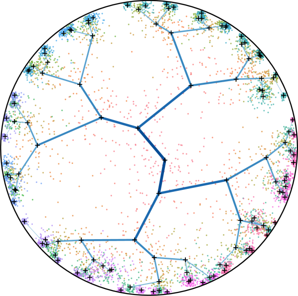
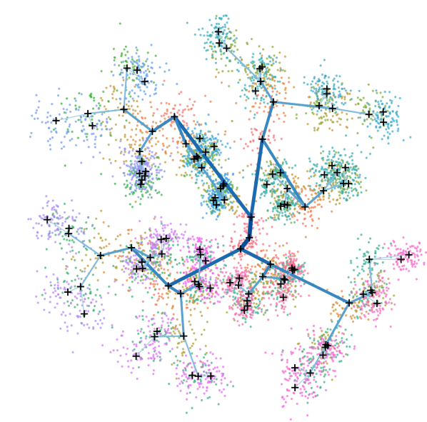
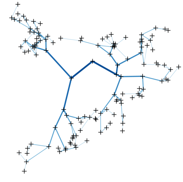
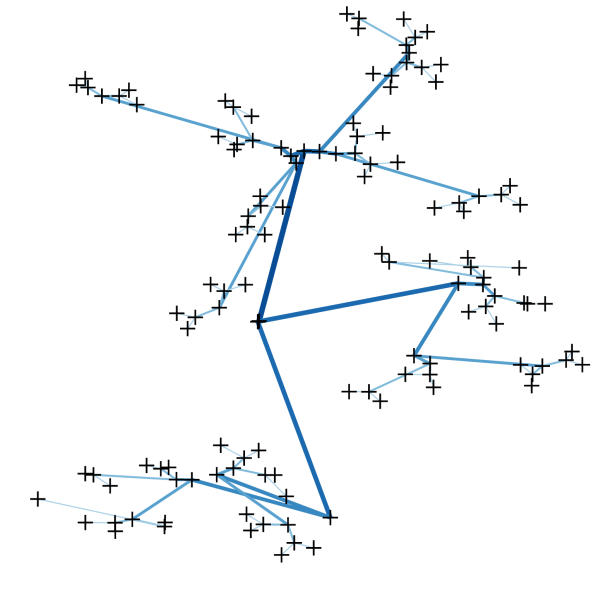
Figure 5: Latent representations learned by – $\mathcal{P}^{1}$-VAE (Leftmost), $\mathcal{N}$-VAE (Center-Left), pca (Center-Right) and gplvm (Rightmost) trained on synthetic dataset. Embeddings are represented by black crosses, and colour dots are posterior samples. Blue lines represent true hierarchy.

We train several $\mathcal{P}^{c}$-VAEs with increasing curvatures, along with a vanilla $\mathcal{N}$-VAE as a baseline. Table 1 shows that the $\mathcal{P}^{c}$-VAE outperforms its Euclidean counterpart in terms of test marginal likelihood. As expected, we observe that the performance of the $\mathcal{N}$-VAE is recovered as the curvature $c$ tends to zero. Also, we notice that increasing the prior distribution distortion $\sigma_{0}$ helps embeddings lie closer to the border, and as a consequence improved generalisation performance. Figure 5 represents latent embeddings for $\mathcal{P}^{1}$-VAE and $\mathcal{N}$-VAE, along with two embedding baselines: principal component analysis (pca) and a Gaussian process latent variable model (gplvm). A hierarchical structure is somewhat learned by all models, yet $\mathcal{P}^{c}$-VAE’s latent representation is the least distorted.

Table 1: Negative test marginal likelihood estimates $\mathcal{L}_{\lx@glossaries@gls@link{acronym}{IWAE}{\leavevmode\textsc{iwae}}}$ (Burda et al.,, 2015) (computed with $5000$ samples) on the synthetic dataset. 95% confidence intervals are computed over 20 trainings.

		Models
	$\sigma_{0}$	$\mathcal{N}$-VAE	$\mathcal{P}^{0.1}$-VAE	$\mathcal{P}^{0.3}$-VAE	$\mathcal{P}^{0.8}$-VAE	$\mathcal{P}^{1.0}$-VAE	$\mathcal{P}^{1.2}$-VAE
$\mathcal{L}_{\lx@glossaries@gls@link{acronym}{IWAE}{\leavevmode\textsc{iwae}}}$	$1$	$57.1_{\pm 0.2}$	$57.1_{\pm 0.2}$	$57.2_{\pm 0.2}$	$56.9_{\pm 0.2}$	$56.7_{\pm 0.2}$	$56.6_{\pm 0.2}$
$\mathcal{L}_{\lx@glossaries@gls@link{acronym}{IWAE}{\leavevmode\textsc{iwae}}}$	$1.7$	$57.0_{\pm 0.2}$	$56.8_{\pm 0.2}$	$56.6_{\pm 0.2}$	$55.9_{\pm 0.2}$	$55.7_{\pm 0.2}$	$\bm{55.6}_{\pm 0.2}$

5.2 Mnist digits

The MNIST (LeCun and Cortes,, 2010) dataset has been used in the literature for hierarchical modelling (Salakhutdinov et al.,, 2011; Saha et al.,, 2018). One can view the natural clustering in MNIST images as a hierarchy with each of the 10 classes being internal nodes of the hierarchy. We empirically assess whether our model can take advantage of such simple underlying hierarchical structure, first by measuring its generalisation capacity via the test marginal log-likelihood. Table 2 shows that our model outperforms its Euclidean counterpart, especially for low latent dimension. This can be interpreted through an information bottleneck perspective; as the latent dimensionality increases, the pressure on the embeddings quality decreases, hence the gain from the hyperbolic geometry is reduced (as observed by Nickel and Kiela, (2017)). Also, by using the Riemannian normal distribution, we achieve slightly better results than with the wrapped normal.

Table 2: Negative test marginal likelihood estimates computed with 5000 samples. 95% confidence intervals are computed over 10 runs. * indicates numerically unstable settings.

		Dimensionality
	c	2	5	10	20
$\mathcal{N}$-VAE	(0)	$144.5_{\pm 0.4}$	$114.7_{\pm 0.1}$	$100.2_{\pm 0.1}$	$97.6_{\pm 0.1}$
$\mathcal{P}$-VAE (Wrapped)	$0.1$	$143.9_{\pm 0.5}$	$115.5_{\pm 0.3}$	$100.2_{\pm 0.1}$	$97.2_{\pm 0.1}$
	$0.2$	$144.2_{\pm 0.5}$	$115.3_{\pm 0.3}$	$100.0_{\pm 0.1}$	$97.1_{\pm 0.1}$
	$0.7$	$143.8_{\pm 0.6}$	$115.1_{\pm 0.3}$	$100.2_{\pm 0.1}$	$97.5_{\pm 0.1}$
	$1.4$	$144.0_{\pm 0.6}$	$114.7_{\pm 0.1}$	$100.7_{\pm 0.1}$	$98.0_{\pm 0.1}$
$\mathcal{P}$-VAE (Riemannian)	$0.1$	$143.7_{\pm 0.6}$	$115.2_{\pm 0.2}$	$99.9_{\pm 0.1}$	$\bm{97.0}_{\pm 0.1}$
	$0.2$	$143.8_{\pm 0.4}$	$114.7_{\pm 0.3}$	$\bm{99.7}_{\pm 0.1}$	$97.4_{\pm 0.1}$
	$0.7$	$143.1_{\pm 0.4}$	$\bm{114.1}_{\pm 0.2}$	$101.2_{\pm 0.2}$	*
	$1.4$	$\bm{142.5}_{\pm 0.4}$	$115.5_{\pm 0.3}$	*	*

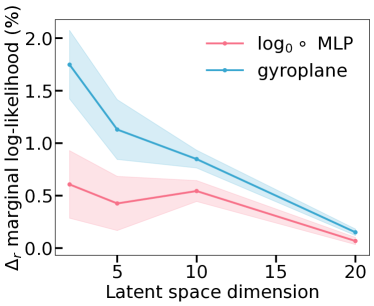
Figure 6: Decoder ablation study on MNIST with wrapped normal $\mathcal{P}^{1}$-VAE. Baseline decoder is a MLP.

We conduct an ablation study to assess the usefulness of the gyroplane layer introduced in Section 3.2. To do so we estimate the test marginal log-likelihood for different choices of decoder. We select a multilayer perceptron (mlp) to be the baseline decoder. We additionally compare to a mlp pre-composed by $\log_{\bm{0}}$, which can be seen as a linearisation of the space around the centre of the ball. Figure 6 shows the relative performance improvement of decoders over the mlp baseline w.r.t. the latent space dimension. We observe that linearising the input of a mlp through the logarithm map slightly improves generalisation, and that using a gyroplane layer as the first layer of the decoder additionally improves generalisation. Yet, these performance gains appear to decrease as the latent dimensionality increases.

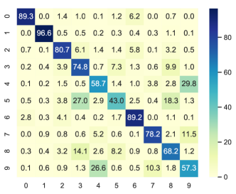
Figure 12: MNIST average confusion matrices of the classifiers trained on embeddings from the $\mathcal{P}^{1.4}$-VAE (Left) and $\mathcal{N}$-VAE (Right) models.

Second, we explore the learned latent representations of the trained $\mathcal{P}$-VAE and $\mathcal{N}$-VAE models shown in Figure 7. Qualitatively our $\mathcal{P}$-VAE produces a clearer partitioning of the digits, in groupings of $\{4,7,9\}$, $\{0,6\}$, $\{2,3,5,8\}$ and $\{1\}$, with right-slanting $\{5,8\}$ being placed separately from the non-slanting ones. Recall that distances increase towards the edge of the Poincaré ball. We quantitatively assess the quality of the embeddings by training a classifier predicting labels. Table 3 shows that the embeddings learned by our $\mathcal{P}$-VAE model yield on average an $2\%$ increase in accuracy over the digits. The full confusion matrices are shown in Figure 12 in Appendix.

Table 3: Per digit accuracy of a classifier trained on the learned latent $2$-d embeddings. Results are averaged over 10 sets of embeddings and 5 classifier trainings.

Digits	0	1	2	3	4	5	6	7	8	9	Avg
$\mathcal{N}$-VAE	89	97	81	75	59	43	89	$\bm{78}$	68	$\bm{57}$	73.6
$\mathcal{P}^{1.4}$-VAE	$\bm{94}$	97	$\bm{82}$	$\bm{79}$	$\bm{69}$	$\bm{47}$	$\bm{90}$	77	68	53	$\bm{75.6}$

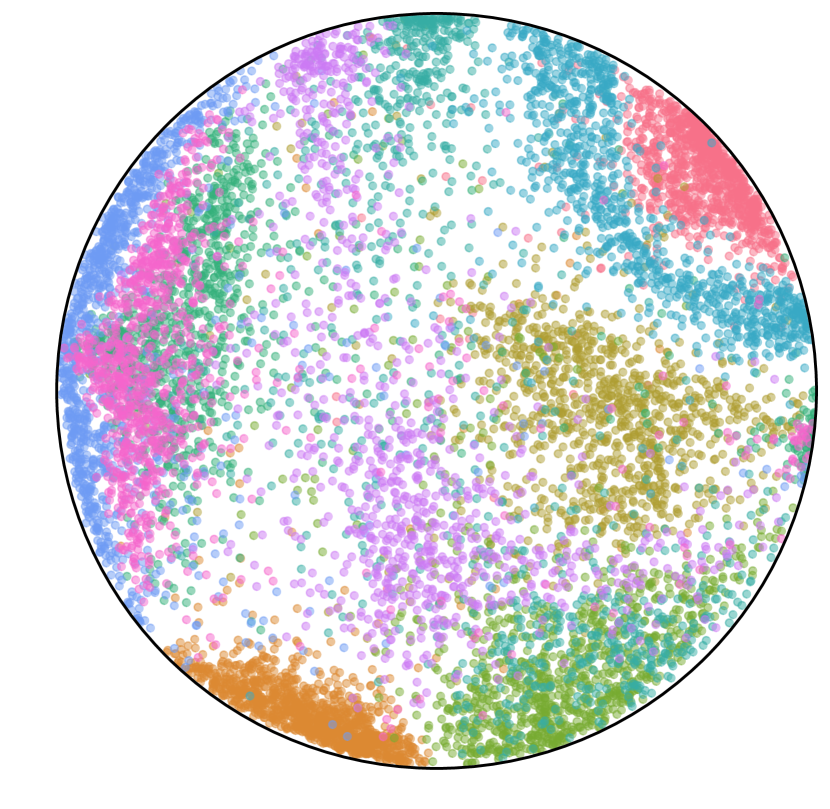
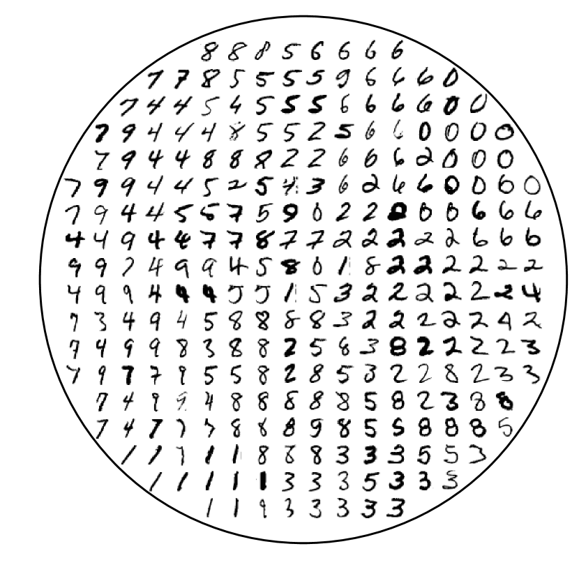
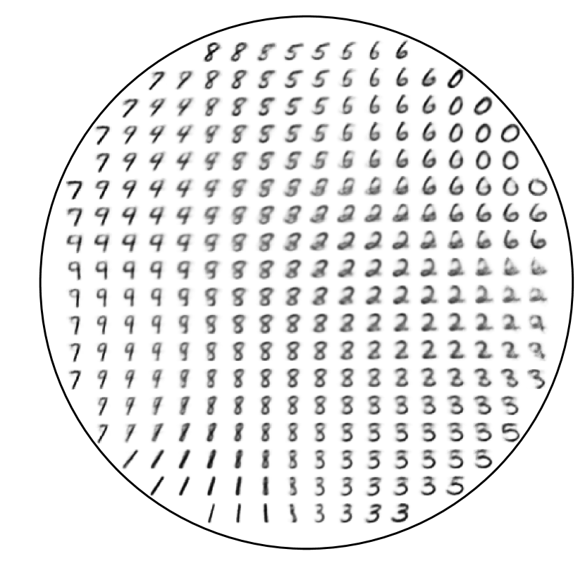
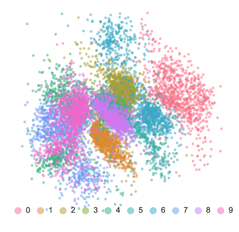
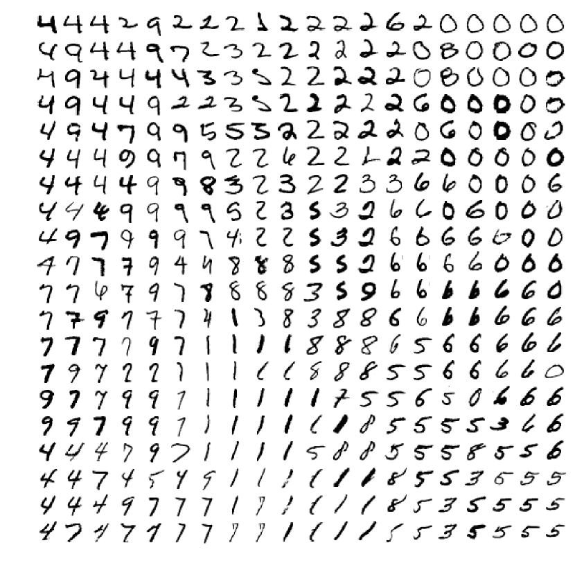
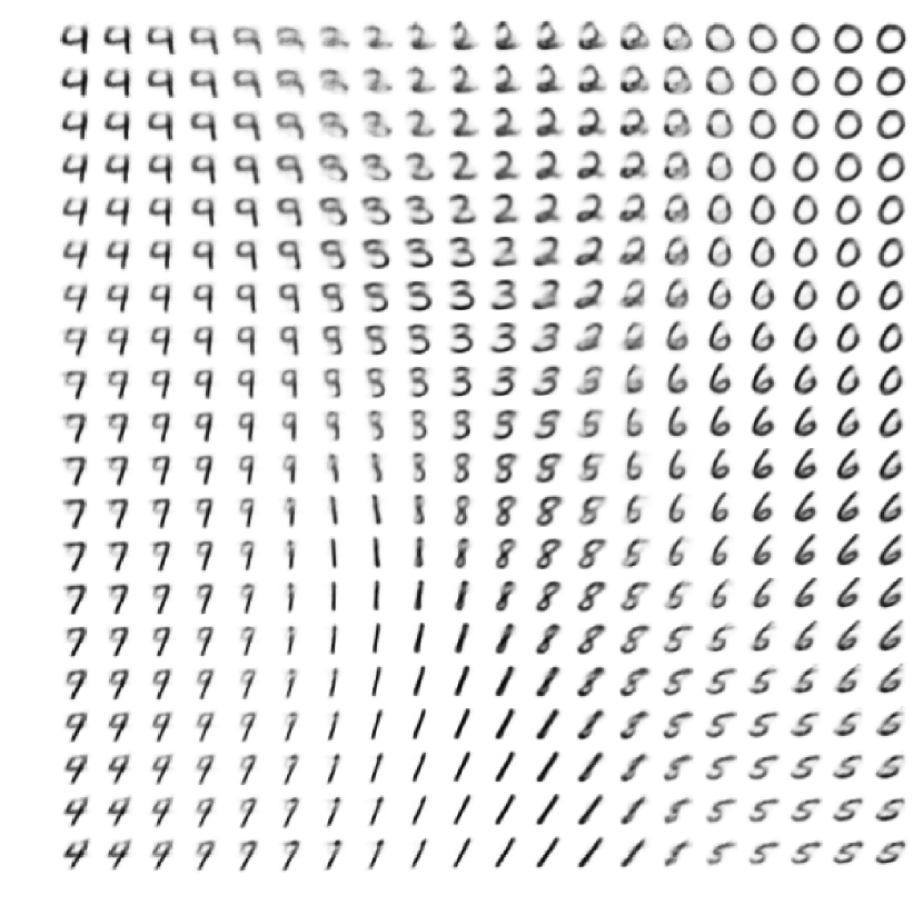
Figure 7: MNIST Posteriors mean (Left) sub-sample of digit images associated with posteriors mean (Middle) Model samples (Right) – for $\mathcal{P}^{1.4}$-VAE (Top) and $\mathcal{N}$-VAE (Bottom).

5.3 Graph embeddings

We evaluate the performance of a variational graph auto-encoder (vgae) (Kipf and Welling,, 2016) with Poincaré ball latent space for link prediction in networks. Edges in complex networks can typically be explained by a latent hierarchy over the nodes (Clauset et al.,, 2008). We believe the Poincaré ball latent space should help in terms of generalisation. We demonstrate these capabilities on three network datasets: a graph of Ph.D. advisor-advisee relationships (Nooy et al.,, 2011), a phylogenetic tree expressing genetic heritage (Hofbauer et al.,, 2016; Sanderson and Eriksson,, 1994) and a biological set representing disease relationships (Goh et al.,, 2007; Rossi and Ahmed,, 2015).

We follow the vgae model, which maps the adjacency matrix $\bm{A}$ to node embeddings $\bm{Z}$ through a graph convolutional network (gcn), and reconstructs $\bm{A}$ by predicting edge probabilities from the node embeddings. In order to take into account the latent space geometry, we parametrise the probability of an edge by $p(\bm{A}_{ij}=1|\bm{z}_{i},\bm{z}_{j})=1-\tanh(d_{\mathcal{M}}(\bm{z}_{i},\bm{z}_{j}))\in(0,1]$ with $d_{\mathcal{M}}$ the latent geodsic metric.

We set the latent dimension to $5$. We follow the training and evaluation procedures introduced in Kipf and Welling, (2016). Models are trained on an incomplete adjacency matrix where some of the edges have randomly been removed. A test set is formed from previously removed edges and an equal number of randomly sampled pairs of unconnected nodes. We report in Table 4 the area under the ROC curve (AUC) and average precision (AP) evaluated on the test set. It can be observed that the $\mathcal{P}$-VAE performs better than its Euclidean counterpart in terms of generalisation to unseen edges.

Table 4: Results on network link prediction. 95% confidence intervals are computed over 40 runs.

	Phylogenetic		CS PhDs		Diseases
	AUC	AP	AUC	AP	AUC	AP
$\mathcal{N}$-VAE	$54.2_{\pm 2.2}$	$54.0_{\pm 2.1}$	$56.5_{\pm 1.1}$	$56.4_{\pm 1.1}$	$89.8_{\pm 0.7}$	$91.8_{\pm 0.7}$
$\mathcal{P}$-VAE	$\bm{59.0_{\pm 1.9}}$	$55.5_{\pm 1.6}$	$\bm{59.8}_{\pm 1.2}$	$56.7_{\pm 1.2}$	$\bm{92.3}_{\pm 0.7}$	$\bm{93.6}_{\pm 0.5}$

6 Conclusion

In this paper we have explored vae s with a Poincaré ball latent space. We gave a thorough treatment of two canonical – wrapped and maximum entropy – normal generalisations on that space, and a rigorous analysis of the difference between the two. We derived the necessary ingredients for training such vae s, namely efficient and reparametrisable sampling schemes, along with probability density functions for these two distributions. We introduced a decoder architecture explicitly taking into account the hyperbolic geometry, and empirically showed that it is crucial for the hyperbolic latent space to be useful. We empirically demonstrated that endowing a vae with a Poincaré ball latent space can be beneficial in terms of model generalisation and can yield more interpretable representations if the data has hierarchical structure.

There are a number of interesting future directions. There are many models of hyperbolic geometry, and several have been considered in a gradient-based setting. Yet, it is still unclear which models should be preferred and which of their properties matter. Also, it would be useful to consider principled ways of assessing whether a given dataset has an underlying hierarchical structure, in the same way that topological data analysis (Pascucci et al.,, 2011) attempts to discover the topologies that underlie datasets.

Acknowledgments

We are extremely grateful to Adam Foster, Phillipe Gagnon and Emmanuel Chevallier for their help. EM, YWT’s research leading to these results received funding from the European Research Council under the European Union’s Seventh Framework Programme (FP7/2007- 2013) ERC grant agreement no. 617071 and they acknowledge Microsoft Research and EPSRC for funding EM’s studentship, and EPSRC grant agreement no. EP/N509711/1 for funding CL’s studentship.

Appendix A Evidence Lower Bound

The elbo can readily be extended for Riemannian latent spaces by applying Jensen’s inequality w.r.t. the metric induced measure $d\mathcal{M}$ which yield

$$\ln p(\bm{x}) =\ln\int_{\mathcal{Z=\mathcal{M}}}p_{\theta}(\bm{x},\bm{z})d\mathcal{M}(\bm{z})=\ln\int_{\mathcal{M}}p_{\theta}(\bm{x}|\bm{z})p(\bm{z})d\mathcal{M}(\bm{z})$$

$$=\ln\int_{\mathcal{M}}\frac{p_{\theta}(\bm{x}|\bm{z})p(\bm{z})}{q_{\phi}(\bm{z}|\bm{x})}q_{\phi}(\bm{z}|\bm{x})d\mathcal{M}(\bm{z})$$

$$\geq\int_{\mathcal{M}}\ln\cfrac{p_{\theta}(\bm{x}|\bm{z})p(\bm{z})}{q_{\phi}(\bm{z}|\bm{x})}\ q_{\phi}(\bm{z}|\bm{x})d\mathcal{M}(\bm{z})$$

$$=\int_{\mathcal{M}}[\ln p_{\theta}(\bm{x}|\bm{z})-\ln p(\bm{z})-\ln q_{\phi}(\bm{z}|\bm{x})]\ q_{\phi}(\bm{z}|\bm{x})\ d\mathcal{M}(\bm{z})$$

$$=\mathbb{E}_{\bm{z}\sim q_{\phi}(\cdot|\bm{x})\mathcal{M}(\cdot)}\left[\ln p_{\theta}(\bm{x}|\bm{z})+\ln p(\bm{z})-\ln q_{\phi}(\bm{z}|\bm{x})\right]$$

$$\triangleq\mathcal{L}_{\mathcal{M}}(\bm{x};\theta,\phi)$$

$$\approx\sum_{k}{\ln p_{\theta}(\bm{x}|\bm{z}^{k})+\ln p(\bm{z}^{k})-\ln q_{\phi}(\bm{z}^{k}|\bm{x})},\quad\bm{z}^{k}\sim q_{\phi}(\cdot|\bm{x})\sqrt{|G(\cdot)|}$$

Appendix B Hyperbolic normal distributions

In this section, we first review some canonical generalisation of the normal distributions to Riemannian manifolds, and then introduce in more details the Riemannian and wrapped normal distributions on the Poincaré ball. Finally, we give architecture and training details about the conducted experiments.

B.1 Probability measures on Riemannian manifolds

Probability measures and random vectors can intrinsically be defined on Riemannian manifolds so as to model uncertainty on non-flat spaces (Pennec,, 2006). The Riemannian metric $G(\bm{z})$ induces an infinitesimal volume element on each tangent space $\mathcal{T}_{\bm{z}}\mathcal{M}$, and thus a measure on the manifold,

$$d\mathcal{M}(\bm{z})=\sqrt{|G(\bm{z})|}d\bm{z},$$ (4)

with $d\bm{z}$ being the Lebesgue measure. Random variables $\bm{z}\in\mathcal{M}$ would naturally be characterised by the Radon-Nikodym derivative of a measure $\nu$ w.r.t. the Riemannian measure $d\mathcal{M}(\cdot)$ (assuming absolute continuity)

$$f(\bm{z})=\frac{d\nu(\bm{z})}{d\mathcal{M}(\bm{z})}.$$

Since the normal distribution plays such a canonical role in statistics, generalising it to manifold is of interest. Given a Fréchet expectation $\bm{\mu}\in\mathcal{M}$ – defined as minimisers of $\int_{\mathcal{M}}d_{\mathcal{M}}(\bm{\mu},\bm{z})^{2}p(\bm{z})d\mathcal{M}(\bm{z})$ – and a dispersion parameter $\sigma>0$ (generally not equal to the standard deviation), several properties ought to be verified by such generalised normal distributions. Such a distribution should tend towards a delta function at $\bm{\mu}$ when $\sigma\rightarrow 0$ and to an (improper for non-compact) uniform distribution when $\sigma\rightarrow\infty$. Also, as the curvature tends to $0$, one should recover the vanilla normal distribution. Hereby, we review canonical generalisations of the normal distribution, which have different theoretical and computational advantages.

Maximum entropy normal

The property that Pennec, (2006) takes for granted is the maximization of the entropy given a mean and a covariance matrix, yielding in the isotropic setting

$$\frac{d\nu^{\text{R}}(\bm{z}|\bm{\mu},\sigma^{2})}{d\mathcal{M}(\bm{z})} =\mathcal{N}^{\text{R}}_{\mathcal{M}}(\bm{z}|\bm{\mu},\sigma^{2})=\frac{1}{Z^{\text{R}}}\exp\left(-\frac{d_{\mathcal{M}}(\bm{\mu},\bm{z})^{2}}{2\sigma^{2}}\right),$$ (5)

with $d_{\mathcal{M}}$ being the Riemannian distance on the manifold induced by the tensor metric. Such a formulation – sometimes referred as Riemannian Normal distribution – is used by Said et al., (2014) in the Poincaré half-plane, or by Hauberg, (2018) in the hypersphere $\mathbb{S}^{d}$. Sampling from such distributions and computing the normalising constant – especially in the anisotropic setting – is usually challenging.

Wrapped normal

Another generalisation is defined by taking the image by the exponential map of a Gaussian distribution on the tangent space centered at the mean value. Such a distribution has been referred in literature as wrapped, push-forward, exp-map or tangential normal distribution. Sampling is therefore straightforward. The pdf is then readily available through the change of variable formula if one can compute the Jacobian of the exponential map (or its inverse). Hence such a distribution is attractive from a computational perspective. Grattarola et al., (2019) and Nagano et al., (2019) rely on such a distribution defined on the hyperboloid model. Wrapped distributions are often encountered in the directional statistics (Ley and Verdebout,, 2017; Hauberg,, 2018).

Restricted normal

What is more, for sub-manifolds of $\mathbb{R}^{n}$, one can consider the restriction of a normal distribution pdf to the manifold. This yields the Von Mises distribution on $\mathbb{S}^{1}$ and the Von Mises-Fisher distribution on $\mathbb{S}^{d}$ (Hauberg,, 2018) and the Stiefel manifold. It is the maximum entropy distribution but with respect to the ambient euclidean metric (Mardia,, 1975).

Diffusion normal

Yet another generalisation arises by defining the normal pdf through the heat kernel, or fundamental solution of the heat equation, $K:\mathbb{R}^{+}\times\mathcal{M}\times\mathcal{M}\rightarrow\mathcal{M}$,

$$\mathcal{N}^{\Delta}_{\mathcal{M}}(\bm{z}|\bm{\mu},\sigma^{2})=K(\sigma^{2}/2,\bm{\mu},\bm{z}).$$ (6)

See for instance Hsu, (2008) for an introduction of Brownian motion on Riemannian manifolds and Paeng, (2011) for conditions on existence and uniqueness of the kernel. Sampling amounts to simulating a Brownian motion, which may be challenging for non sub-manifolds of $\mathbb{R}^{n}$. Closed form solutions of the heat kernel is available for some manifolds such as spheres or flat tori, otherwise numerical approximations can be used. Such a distribution has been used in a vae setting (Rey et al.,, 2019; Li et al.,, 2019).

Other than normal distributions

Of course one needs not to restrict itself to generalisations of the normal distribution. For instance, one could consider a wrapped spherical Student-t as $\bm{z}\sim\exp_{\bm{\mu}\#}S_{t}(0,\nu)$ or a Riemannian Student-t with density proportional to $\left(1+d_{\mathcal{M}}(\bm{z},\bm{\mu})^{2}/\nu\right)^{(-\nu+1)/2}$ (by making sure that this density is $d\mathcal{M}$-integrable).

B.2 Hyperbolic polar coordinates

In this subsection, we review the hyperbolic polar change of coordinates allowing us to reparametrise hyperbolic normal distributions in a similar fashion than the Box–Muller transform (Box and Muller,, 1958).

Polar coordinates

Euclidean polar coordinates, express points $\bm{z}\in\mathbb{R}^{d}$ through a radius $r\geq 0$ and a direction $\bm{\alpha}\in\mathbb{S}^{d-1}$ such that $\bm{z}=r\bm{\alpha}$. Yet, one could choose another pole (or reference point) $\bm{\mu}\neq\bm{0}$ such that $\bm{z}=\bm{\mu}+r\bm{\alpha}$. Consequently, $r=d_{E}(\bm{\mu},\bm{z})$. An analogous change of variables can also be constructed in Riemannian manifolds relying on the exponential map instead of the addition operator. Given a pole $\bm{\mu}\in\mathbb{B}_{c}^{d}$, the point of hyperbolic polar coordinates $\bm{z}=(r,\bm{\alpha})$ is defined as $\bm{z}=\gamma(r)$, with $r=d^{c}_{p}(\bm{\mu},\bm{z})$ and $\gamma:\mathbb{R}^{+}\rightarrow\mathbb{B}_{c}^{d}$ a curve such that $\gamma^{\prime}(0)=\bm{\alpha}\in\mathbb{S}^{d-1}$. Hence $\bm{z}=\exp^{c}_{\bm{\mu}}\left(\frac{r}{\lambda^{c}_{\bm{\mu}}}\bm{\alpha}\right)$ since $d^{c}_{p}(\bm{\mu},\bm{z})=\|\ln^{c}_{\bm{\mu}}(x)\|_{\bm{\mu}}=\|\frac{r}{\lambda^{c}_{\bm{\mu}}}\bm{\alpha}\|_{\bm{\mu}}=r$.

Tensor metric

We derive below the expression of the Poincaré ball metric in such hyperbolic polar coordinate, for the specific setting where $\bm{\mu}=\bm{0}$: $\bm{z}=\exp^{c}_{\bm{0}}(\frac{r}{2}\bm{\alpha})$. Switching to Euclidean polar coordinate we get

$$ds^{2}_{\mathbb{B}_{c}^{d}} =(\lambda^{c}_{\bm{z}})^{2}(dz_{1}^{2}+\dots+dz_{d}^{2})=\frac{4}{\left(1-c\|x\|^{2}\right)^{2}}d\bm{z}^{2}$$

$$=\frac{4}{(1-c\rho^{2})^{2}}(d\rho^{2}+\rho^{2}ds^{2}_{\mathbb{S}^{d-1}}).$$ (7)

Let’s define $r=d^{c}_{p}(\bm{0},\bm{z})=L(\gamma)$, with $\gamma$ being the geodesic joining $\bm{0}$ and $\bm{z}$. Since such a geodesic is the segment $[\bm{0},\bm{z}]$, we have

$$r=\int_{0}^{\rho}\lambda_{t}^{c}dt=\int_{0}^{\rho}\frac{2}{1-ct^{2}}dt=\int_{0}^{\sqrt{c}\rho}\frac{2}{1-t^{2}}\frac{dt}{\sqrt{c}}=\frac{2}{\sqrt{c}}\tanh^{-1}(\sqrt{c}\rho).$$

Plugging $\rho=\frac{1}{\sqrt{c}}\tanh(\sqrt{c}\frac{r}{2})$ (and $d\rho=(1-c\rho^{2})/2dr$) into Eq 7 yields

$$ds^{2}_{\mathbb{B}_{c}^{d}} =\frac{4}{(1-c\rho^{2})^{2}}\frac{1}{4}(1-c\rho^{2})^{2}dr^{2}+\left(2\frac{\rho}{1-c\rho^{2}}\right)^{2}ds^{2}_{\mathbb{S}^{d-1}}$$

$$=dr^{2}+\left(2\frac{\frac{1}{\sqrt{c}}\tanh(\sqrt{c}\frac{r}{2})}{1-c\left(\frac{1}{\sqrt{c}}\tanh(\sqrt{c}\frac{r}{2}\right)^{2}}\right)^{2}ds^{2}_{\mathbb{S}^{d-1}}$$

$$=dr^{2}+\left(\frac{1}{\sqrt{c}}\sinh(\sqrt{c}r)\right)^{2}ds^{2}_{\mathbb{S}^{d-1}}.$$ (8)

The Euclidean line element is recovered when $c\rightarrow 0$

$$ds^{2}_{\mathbb{R}^{d}}=dr^{2}+r^{2}ds^{2}_{\mathbb{S}^{d-1}}.$$ (9)

In an appropriate orthonormal basis of $\mathcal{T}_{\bm{\mu}}\mathbb{B}_{c}^{d}$, the hyperbolic polar coordinate leads to the following expression of the matrix of the metric

$$G(\bm{z})=\begin{pmatrix}1&0\\ 0&\left(\frac{\sinh(\sqrt{c}r)}{\sqrt{c}r}\right)^{2}\bm{I}_{d-1}\end{pmatrix}.$$ (10)

Hence, the density of the Riemannian measure with respect to the image of the Lebesgue measure of $\mathcal{T}_{\bm{\mu}}\mathbb{B}_{c}^{d}$ by $\exp^{c}_{\bm{\mu}}$ is given by

$$\sqrt{|G(\bm{z})|}=\left(\frac{\sinh(\sqrt{c}r)}{\sqrt{c}r}\right)^{d-1}.$$ (11)

This result holds for any reference point $\bm{\mu}\in\mathbb{B}_{c}^{d}$, with $r=d^{c}_{p}(\bm{\mu},\bm{z})$, since the metric induced measure is invariant under the isometries of the manifold (i.e. Möbius transformations). This result can also be found in Chevallier et al., (2015); Said et al., (2014). Also, the fact that the line element $ds^{2}_{\mathbb{B}_{c}^{d}}$ and equivalently the metric $G$ only depends on the radius in hyperbolic polar coordinate, is a consequence of the hyperbolic space’s isotropy.

Integration

We now make use of the aforementioned hyperbolic polar coordinates to integrate functions following Said et al., (2014). The integral of a function $f:\mathbb{B}_{c}^{d}\rightarrow\mathbb{R}$ can be computed by using polar coordinates,

$$\int_{\mathbb{B}_{c}^{d}}f(\bm{z})d\mathcal{M}(\bm{z}) =\int_{\mathbb{B}_{c}^{d}}f(\bm{z})\sqrt{|G(\bm{z})|}\ d\bm{z}$$

$$=\int_{\mathcal{T}_{\bm{\mu}}\mathbb{B}_{c}^{d}\cong\mathbb{R}^{d}}f(\bm{v})\sqrt{|G(\bm{v})|}\ d\bm{v}$$ (12)

$$=\int_{\mathbb{R}_{+}}\int_{\mathbb{S}^{d-1}}f(r)\sqrt{|G(r)|}dr~{}r^{d-1}~{}ds_{\mathbb{S}^{d-1}}$$

$$=\int_{\mathbb{R}_{+}}\int_{\mathbb{S}^{d-1}}f(r)\left(\frac{\sinh(\sqrt{c}r)}{\sqrt{c}r}\right)^{d-1}dr~{}r^{d-1}~{}ds_{\mathbb{S}^{d-1}}$$

$$=\int_{\mathbb{R}_{+}}\int_{\mathbb{S}^{d-1}}f(r)\left(\frac{\sinh(\sqrt{c}r)}{\sqrt{c}}\right)^{d-1}dr~{}ds_{\mathbb{S}^{d-1}}.$$ (13)

B.3 Wrapped hyperbolic normal distribution on $\mathbb{B}_{c}^{d}$

Anisotropic

The wrapped normal distribution considers a normal distribution in the tangent space $\mathcal{T}_{\bm{\mu}}\mathbb{B}_{c}^{d}$ being pushed-forward along the exponential map. One can obtain sampled as follow

$$\bm{z}=\exp^{c}_{\bm{\mu}}\left(G(\bm{\mu})^{-\frac{1}{2}}~{}\bm{v}\right)=\exp^{c}_{\bm{\mu}}\left(\frac{\bm{v}}{\lambda^{c}_{\bm{\mu}}}\right),\ \text{with}\ \bm{\bm{v}}\sim\mathcal{N}(\cdot|\bm{0},\Sigma).$$ (14)

Then, its density is given by

$$\mathcal{N}^{\text{W}}_{\mathbb{B}_{c}^{d}}(\bm{z}|\bm{\mu},\Sigma) =\mathcal{N}\left(G(\bm{\mu})^{1/2}\log_{\bm{\mu}}(\bm{z})~{}\middle|~{}\bm{0},\Sigma\right)\bigg{(}\frac{\sqrt{c}~{}d_{p}^{c}(\bm{\mu},\bm{z})}{\sinh(\sqrt{c}~{}d_{p}^{c}(\bm{\mu},\bm{z}))}\bigg{)}^{d-1}$$

$$=\mathcal{N}\left(\lambda^{c}_{\bm{\mu}}~{}\log_{\bm{\mu}}(\bm{z})~{}\middle|~{}\bm{0},\Sigma\right)\bigg{(}\frac{\sqrt{c}~{}d_{p}^{c}(\bm{\mu},\bm{z})}{\sinh(\sqrt{c}~{}d_{p}^{c}(\bm{\mu},\bm{z}))}\bigg{)}^{d-1}$$ (15)

with $G(\bm{\mu})^{1/2}$ the unique square-root matrix of $G(\bm{\mu})$ (thanks to the positive definiteness of the metric tensor). This can be shown by plugging this density as $f$ in Equation (12) with $\bm{v}=r\bm{\alpha}=\lambda^{c}_{\bm{\mu}}\log_{\bm{\mu}}(\bm{z})$, we get

$$\int_{\mathbb{B}_{c}^{d}}\mathcal{N}^{\text{W}}_{\mathbb{B}_{c}^{d}}(\bm{z}|\bm{\mu},\Sigma)~{}d\mathcal{M}(\bm{z}) =\int_{\mathcal{T}_{\bm{\mu}}\mathbb{B}_{c}^{d}\cong\mathbb{R}^{d}}\mathcal{N}\left(\bm{v}~{}\middle|~{}\bm{0},\Sigma\right)\bigg{(}\frac{\sqrt{c}~{}\left\|\bm{v}\right\|_{2}}{\sinh(\sqrt{c}~{}\left\|\bm{v}\right\|_{2})}\bigg{)}^{d-1}\sqrt{|G(\bm{v})|}~{}d\bm{v}$$

$$=\int_{\mathbb{R}^{d}}\mathcal{N}\left(\bm{v}~{}\middle|~{}\bm{0},\Sigma\right)\bigg{(}\frac{\sqrt{c}~{}\left\|\bm{v}\right\|_{2}}{\sinh(\sqrt{c}~{}\left\|\bm{v}\right\|_{2})}\bigg{)}^{d-1}\left(\frac{\sinh(\sqrt{c}\left\|\bm{v}\right\|_{2})}{\sqrt{c}\left\|\bm{v}\right\|_{2}}\right)^{d-1}~{}d\bm{v}$$

$$=\int_{\mathbb{R}^{d}}\mathcal{N}\left(\bm{v}~{}\middle|~{}\bm{0},\Sigma\right)~{}d\bm{v}.$$

Figure 8: Anisotropic wrapped normal probability measures for Fréchet means $\bm{\mu}$ (red +), concentrations $\Sigma=\text{diag}(\bm{\sigma})$ and $c=1$.

Isotropic

In the isotropic setting, we therefore get

$$\int_{\mathbb{B}_{c}^{d}}\mathcal{N}^{\text{W}}_{\mathbb{B}_{c}^{d}}(\bm{z}|\bm{\mu},\sigma^{2})~{}d\mathcal{M}(\bm{z}) =\int_{\mathbb{R}_{+}}\int_{\mathbb{S}^{d-1}}\frac{1}{Z^{\text{R}}}e^{-\frac{r^{2}}{2\sigma^{2}}}r^{d-1}dr~{}ds_{\mathbb{S}^{d-1}}.$$ (16)

The hyperbolic radius $r=d_{p}^{c}(\bm{\mu},\bm{z})$ consequently follows the usual $\chi$ distribution with density

$$\rho^{\text{W}}(r)\propto\mathbb{1}_{\mathbb{R}_{+}}(r)~{}e^{-\frac{r^{2}}{2\sigma^{2}}}r^{d-1},$$ (17)

and the density of the wrapped normal given by

$$\mathcal{N}^{\text{W}}_{\mathbb{B}_{c}^{d}}(\bm{z}|\bm{\mu},\sigma^{2})=\frac{d\nu^{\text{W}}(\bm{z}|\bm{\mu},\sigma^{2})}{d\mathcal{M}(\bm{z})} =(2\pi\sigma^{2})^{-d/2}\exp\left(-\frac{d_{p}^{c}(\bm{\mu},\bm{z})^{2}}{2\sigma^{2}}\right)\bigg{(}\frac{\sqrt{c}~{}d_{p}^{c}(\bm{\mu},\bm{z})}{\sinh(\sqrt{c}~{}d_{p}^{c}(\bm{\mu},\bm{z}))}\bigg{)}^{d-1}.$$

B.4 Maximum entropy hyperbolic normal distribution on $\mathbb{B}_{c}^{d}$

Alternatively, by considering the maximum entropy generalisation of the normal distribution one gets (Pennec,, 2006)

$$\mathcal{N}^{\text{R}}_{\mathbb{B}_{c}^{d}}(\bm{z}|\bm{\mu},\sigma^{2})=\frac{d\nu^{\text{R}}(\bm{z}|\bm{\mu},\sigma^{2})}{d\mathcal{M}(\bm{z})}=\frac{1}{Z^{\text{R}}}\exp\left(-\frac{d_{p}^{c}(\bm{\mu},\bm{z})^{2}}{2\sigma^{2}}\right).$$ (18)

Such a pdf can be computed pointwise once $Z^{\text{R}}$ is known, which we derive in Appendix B.4.3. Also, we observe that as $c$ and $\sigma$ get smaller (resp. bigger), the Riemannian normal pdf gets closer (resp. further) to the wrapped normal pdf.

B.4.1 Reparametrisation

Plugging the Riemannian normal density as $f$ in Equation (13), with $r=d^{c}_{p}(\bm{\mu},\bm{z})$, we have

$$\int_{\mathbb{B}_{c}^{d}}\mathcal{N}^{\text{R}}_{\mathbb{B}_{c}^{d}}(\bm{z}|\bm{\mu},\sigma^{2})~{}d\mathcal{M}(\bm{z}) =\int_{\mathbb{R}_{+}}\int_{\mathbb{S}^{d-1}}\frac{1}{Z^{\text{R}}}e^{-\frac{r^{2}}{2\sigma^{2}}}\left(\frac{\sinh(\sqrt{c}r)}{\sqrt{c}}\right)^{d-1}dr~{}ds_{\mathbb{S}^{d-1}}$$

$$=\frac{1}{Z^{\text{R}}}\left(\int_{\mathbb{R}_{+}}e^{-\frac{r^{2}}{2\sigma^{2}}}\left(\frac{\sinh(\sqrt{c}r)}{\sqrt{c}}\right)^{d-1}dr\right)\left(\int_{\mathbb{S}^{d-1}}ds_{\mathbb{S}^{d-1}}\right)$$ (19)

Hence, samples $\bm{z}\sim\mathcal{N}^{\text{R}}_{\mathcal{M}}(\bm{z}|\bm{\mu},\sigma^{2})d\mathcal{M}(\bm{z})$ can be reparametrised as

$$\bm{z}=\exp^{c}_{\bm{\mu}}\left(\frac{r}{\lambda^{c}_{\bm{\mu}}}\bm{\alpha}\right)$$ (20)

with the direction $\bm{\alpha}$ being uniformly distributed on the hypersphere $\mathbb{S}^{d-1}$, i.e.

$$\bm{\alpha}\sim\mathcal{U}(\mathbb{S}^{d-1})$$

and the hyperbolic radius $r=d^{c}_{p}(\bm{\mu},\bm{z})$ distributed according to the following density (w.r.t the Lebesgue measure)

$$\rho^{\text{R}}(r)=\frac{\mathbb{1}_{\mathbb{R}_{+}}(r)}{Z^{\text{R}}_{r}}e^{-\frac{r^{2}}{2\sigma^{2}}}\left(\frac{\sinh(\sqrt{c}r)}{\sqrt{c}}\right)^{d-1}.$$ (21)

Developed expression

By expanding the $\sinh$ term using the binomial formula, we get

$$\rho^{\text{R}}(r) =\frac{\mathbb{1}_{\mathbb{R}_{+}}(r)}{Z^{\text{R}}_{r}}e^{-\frac{r^{2}}{2\sigma^{2}}}\left(\frac{\sinh(\sqrt{c}r)}{\sqrt{c}}\right)^{d-1}$$

$$=\frac{\mathbb{1}_{\mathbb{R}_{+}}(r)}{Z^{\text{R}}_{r}}e^{-\frac{r^{2}}{2\sigma^{2}}}\left(\frac{e^{\sqrt{c}r}-e^{-\sqrt{c}r}}{2\sqrt{c}}\right)^{d-1}$$

$$=\frac{\mathbb{1}_{\mathbb{R}_{+}}(r)}{Z^{\text{R}}_{r}}e^{-\frac{r^{2}}{2\sigma^{2}}}\frac{1}{(2\sqrt{c})^{d-1}}\sum_{k=0}^{d-1}{d-1\choose k}\left(e^{\sqrt{c}r}\right)^{d-1-k}\left(-e^{-\sqrt{c}r}\right)^{k}$$

$$=\frac{\mathbb{1}_{\mathbb{R}_{+}}(r)}{Z^{\text{R}}_{r}}\frac{1}{(2\sqrt{c})^{d-1}}e^{-\frac{r^{2}}{2\sigma^{2}}}\sum_{k=0}^{d-1}\left(-1\right)^{k}{d-1\choose k}e^{(d-1-2k)\sqrt{c}r}$$

$$=\frac{\mathbb{1}_{\mathbb{R}_{+}}(r)}{Z^{\text{R}}_{r}}\frac{1}{(2\sqrt{c})^{d-1}}\sum_{k=0}^{d-1}\left(-1\right)^{k}{d-1\choose k}e^{-\frac{r^{2}}{2\sigma^{2}}+(d-1-2k)\sqrt{c}r}$$

$$=\frac{\mathbb{1}_{\mathbb{R}_{+}}(r)}{Z^{\text{R}}_{r}}\frac{1}{(2\sqrt{c})^{d-1}}\sum_{k=0}^{d-1}\left(-1\right)^{k}{d-1\choose k}e^{\frac{(d-1-2k)^{2}}{2}c\sigma^{2}}e^{-\frac{1}{2\sigma^{2}}\left[r-(d-1-2k)\sqrt{c}\sigma^{2}\right]^{2}}.$$ (22)

B.4.2 Sampling

In this section we detail the sampling scheme that we use for the Riemannian normal distribution $\mathcal{N}^{\text{R}}_{\mathbb{B}_{c}^{d}}(\cdot|\bm{\mu},\sigma^{2})$, along with a reparametrisation which allows to compute gradients with respect to the parameters $\bm{\mu}$ and $\sigma$.

Sampling challenges due to the hyperbolic geometry

Several properties of the Euclidean space do not generalise to the hyperbolic setting, unfortunately hardening the task of obtaining samples from Riemannian normal distributions. First, one can factorise a normal density through the space’s dimensions – thanks to to the Pythagorean theorem – hence allowing to divide the task on several subspaces and then concatenate the samples. Such a property does not extend to the hyperbolic geometry, thus seemingly preventing us from focusing on $2$-dimensional samples. Second, in Euclidean geometry, the polar radius $r$ is distributed according to $\rho^{\text{W}}(r)=\frac{\mathbb{1}_{\mathbb{R}_{+}}(r)}{Z_{r}}e^{-\frac{r^{2}}{2\sigma^{2}}}r^{d-1}$, making it easy by a linear change of variable to take into account different scaling values. The non-linearity of $\sinh$ prevent us from using such a simple change of variable.

Computing gradients with respect to parameters

So as to compute gradients of samples $\bm{z}$ with respect to the parameters $\bm{\mu}$ and $\sigma$ of samples of a hyperbolic distributions, we respectively rely on the reparametrisation given by Eq 20 for $\nabla_{\bm{\mu}}\bm{z}$, and on an implicit reparametrisation (Figurnov et al.,, 2018) of $r$ for $\nabla_{\sigma}\bm{z}$. We have $\bm{z}=\exp^{c}_{\bm{\mu}}\left(\frac{r}{\lambda^{c}_{\bm{\mu}}}\bm{\alpha}\right)$ with $\bm{\alpha}\sim\mathcal{U}(\mathbb{S}^{d-1})$ and $r\sim\rho^{\text{R}}(\cdot)$. Hence,

$$\nabla_{\bm{\mu}}\bm{z}=\nabla_{\bm{\mu}}\exp^{c}_{\bm{\mu}}(\bm{u}),$$ (23)

with $\bm{u}=\frac{r}{\lambda^{c}_{\bm{\mu}}}\bm{\alpha}$ (actually) independent of $\bm{\mu}$, and

$$\nabla_{\sigma}\bm{z}=\nabla_{\sigma}\exp^{c}_{\bm{\mu}}(\bm{u})=\nabla_{\bm{u}}\exp^{c}_{\bm{\mu}}(\bm{u})\frac{\bm{\alpha}}{\lambda^{c}_{\bm{\mu}}}\nabla_{\sigma}r,$$ (24)

with $\nabla_{\sigma}(r)$ computed via the implicit reparametrisation given by

$$\nabla_{\sigma}(r) =-\left(\nabla_{r}F^{\text{R}}(r,\sigma)\right)^{-1}\nabla_{\sigma}F^{\text{R}}(r,\sigma)$$

$$=-\left(\rho^{\text{R}}(r;\sigma)\right)^{-1}\nabla_{\sigma}F^{\text{R}}(r,\sigma).$$ (25)

Sampling hyperbolic radii

Unfortunately the density of the hyperbolic radius $\rho^{\text{R}}(r)$ is not a well-known distribution and its cumulative density function does not seem analytically invertible. We therefore rely on rejection sampling methods.

Adaptive Rejection Sampling

By making use of the log-concavity of $\rho^{\text{R}}$, we can rely on a piecewise exponential distribution proposal from adaptive rejection sampling (ars) (R. Gilks and Wild,, 1992). Such a proposal automatically adapt itself with respect to the parameters $\sigma$, $c$ and $d$. Even though $\mathcal{N}_{\mathbb{B}_{c}^{d}}$ is defined on a d-dimensional manifold, $\rho^{\text{R}}$ is a univariate distribution hence the sampling scheme is not directly affected by dimensionality. The difficulty in ars is to choose the initial set of points to construct the piecewise exponential proposal. To do so, we first compute the mean $m=\mathbb{E}_{r\sim\rho^{\text{R}}}[r]$ and standard deviation $s=\mathbb{V}_{r\sim\rho^{\text{R}}}[r]^{1/2}$ of the targeted distribution. Then we choose a grid $\eta=(\eta_{1},\dots,\eta_{K})=\left(\text{linspace}(\eta_{max},\eta_{min},K/2),\ \text{linspace}(\eta_{min},\eta_{max},K/2)\right)$. Eventually, we set the initial points $(x_{1},\dots,x_{K})$ to $x_{k}=m+\eta_{k}*\min(s,0.95*m/\eta_{max})$. For our experiments we chose $\eta_{min}=.1,\eta_{max}=3,K=20$. We do not adapt the proposal within the rejection sampling since we empirically found it unnecessary.

Alternatively, we derived bellow two non-adaptive proposal distributions along with their rejection rate constants. Yet, we observe that these rates do not scale well the dimensionality $d$ and distortion $\sigma$, making them ill-suited for practical purposes.

Rejection Sampling with truncated Normal proposal

The developed expression of $\rho(r)^{\text{R}}$ from Eq (22) highlights the fact that the density can immediately be upper bounded by a truncated normal density:

$$\rho(r)^{\text{R}} =\frac{\mathbb{1}_{\mathbb{R}_{+}}(r)}{Z^{\text{R}}_{r}}\frac{1}{(2\sqrt{c})^{d-1}}\sum_{k=0}^{d-1}\left(-1\right)^{k}{d-1\choose k}e^{\frac{(d-1-2k)^{2}}{2}c\sigma^{2}}e^{-\frac{1}{2\sigma^{2}}\left[r-(d-1-2k)\sqrt{c}\sigma^{2}\right]^{2}}$$

$$\leq\frac{\mathbb{1}_{\mathbb{R}_{+}}(r)}{Z^{\text{R}}_{r}}\frac{1}{(2\sqrt{c})^{d-1}}\sum_{2k=0}^{d-1}{d-1\choose 2k}e^{\frac{(d-1-4k)^{2}}{2}c\sigma^{2}}e^{-\frac{1}{2\sigma^{2}}\left[r-(d-1-4k)\sqrt{c}\sigma^{2}\right]^{2}}.$$

Then we choose our proposal $g$ to be the truncated normal distribution associated with $k=0$, i.e. with mean $(d-1)\sqrt{c}\sigma^{2}$ and variance $\sigma^{2}$

$$g(r) =\frac{\mathbb{1}_{r>0}}{\sigma\left(1-\Phi\left(-\frac{(d-1)\sqrt{c}\sigma^{2}}{\sigma}\right)\right)}\frac{1}{\sqrt{2\pi}}e^{-\frac{1}{2\sigma^{2}}\left(r-(d-1)\sqrt{c}\sigma^{2}\right)^{2}}$$

$$=\frac{1}{\sqrt{2\pi}}\frac{\mathbb{1}_{r>0}}{\sigma\left(1-\frac{1}{2}-\frac{1}{2}\text{erf}\left(-(d-1)\sqrt{c}\frac{\sigma}{\sqrt{2}}\right)\right)}e^{-\frac{1}{2\sigma^{2}}\left(r-(d-1)\sqrt{c}\sigma^{2}\right)^{2}}$$

$$=\sqrt{\frac{2}{\pi}}\frac{\mathbb{1}_{r>0}}{\sigma\left(1+\text{erf}\left(\frac{(d-1)\sqrt{c}\sigma}{\sqrt{2}}\right)\right)}e^{-\frac{1}{2\sigma^{2}}\left(r-(d-1)\sqrt{c}\sigma^{2}\right)^{2}}$$

$$=\frac{\mathbb{1}_{r>0}}{Z_{g}(\sigma)}e^{-\frac{1}{2\sigma^{2}}\left(r-(d-1)\sqrt{c}\sigma^{2}\right)^{2}}$$ (26)

with

$$Z_{g}=\sqrt{\frac{\pi}{2}}\sigma\left(1+\text{erf}\left(\frac{(d-1)\sqrt{c}\sigma}{\sqrt{2}}\right)\right).$$ (27)

Computing the ratio of the densities yield

$$\frac{\rho(r)^{\text{R}}}{g(r)} =\frac{Z_{g}(\sigma)}{Z^{\text{R}}_{r}}\frac{1}{(2\sqrt{c})^{d-1}}\sum_{k=0}^{d-1}\left(-1\right)^{k}{d-1\choose k}e^{\frac{(d-1-2k)^{2}}{2}c\sigma^{2}}e^{-\frac{1}{2\sigma^{2}}\left[r-(d-1-2k)\sqrt{c}\sigma^{2}\right]^{2}}e^{+\frac{1}{2\sigma^{2}}\left[r-(d-1)\sqrt{c}\sigma^{2}\right]^{2}}$$

$$=\frac{Z_{g}(\sigma)}{Z^{\text{R}}_{r}}\frac{1}{(2\sqrt{c})^{d-1}}\sum_{k=0}^{d-1}\left(-1\right)^{k}{d-1\choose k}e^{\frac{(d-1-2k)^{2}}{2}c\sigma^{2}}e^{2k\sqrt{c}\left((d-1-k)\sqrt{c}\sigma^{2}-r\right)}.$$

Hence

$$\rho(r)^{\text{R}}/g(r)\leq M\triangleq\frac{Z_{g}(\sigma)}{Z^{\text{R}}_{r}}\frac{1}{(2\sqrt{c})^{d-1}}e^{\frac{(d-1)^{2}c\sigma^{2}}{2}}.$$ (28)

Rejection Sampling with Gamma proposal

Now let’s consider the following $\text{Gamma}(2,\sigma)$ density:

$$g(r) =\frac{\mathbb{1}_{r>0}}{Z_{g}(\sigma)}re^{-\frac{r}{\sigma}}$$

with

$$Z_{g}(\sigma) =\Gamma(2)\sigma^{2}.$$

Then log ratio of the densities can be upper bounded as following:

$$\ln\left(\frac{\rho(r)^{\text{R}}}{g(r)}\right) =\ln\frac{Z_{g}(\sigma)}{Z^{\text{R}}_{r}}-\frac{r^{2}}{2\sigma^{2}}+(d-1)\ln(e^{\sqrt{c}r}-e^{-\sqrt{c}r})-(d-1)\ln 2-\ln r+\frac{r}{\sigma}$$

$$=\ln\frac{Z_{g}(\sigma)}{Z^{\text{R}}_{r}}-(d-1)\ln 2\underbrace{-\frac{r^{2}}{2\sigma^{2}}+\left((d-1)\sqrt{c}+\frac{1}{\sigma}\right)r}_{\leq\frac{((d-1)\sqrt{c}\sigma+1)^{2}}{2}}+\underbrace{(d-1)\ln\left(\frac{1-e^{-2\sqrt{c}r}}{r}\right)}_{\leq(d-1)\ln(2\sqrt{c})}$$

$$\leq\ln\frac{Z_{g}(\sigma)}{Z^{\text{R}}_{r}}+\frac{((d-1)\sqrt{c}\sigma+1)^{2}}{2}+(d-1)\ln{\sqrt{c}}.$$

Hence

$$\rho(r)^{\text{R}}/g(r)\leq M\triangleq\frac{Z_{g}(\sigma)}{Z^{\text{R}}_{r}}c^{\frac{d-1}{2}}e^{\frac{((d-1)\sqrt{c}\sigma+1)^{2}}{2}}.$$ (29)

B.4.3 Normalisation constant

In order to evaluate the density of the Riemannian normal distribution, we need to compute the normalisation constant, which we derive in this subsection.

Cumulative density function

First let’s derive the cumulative density function of the hyperbolic radius. Integrating the expended density of Eq (22) yields

$$F^{\text{R}}_{r}(r) =\int_{-\infty}^{r}\rho^{\text{R}}(r)dr$$

$$=\frac{1}{Z^{\text{R}}_{r}}\frac{1}{(2\sqrt{c})^{d-1}}\sum_{k=0}^{d-1}\left(-1\right)^{k}{d-1\choose k}e^{\frac{(d-1-2k)^{2}}{2}c\sigma^{2}}$$

$$\hskip 20.00003pt\times\int_{0}^{r}e^{-\frac{1}{2\sigma^{2}}\left[r-(d-1-2k)\sqrt{c}\sigma^{2}\right]^{2}}dr\sum_{k=0}^{d-1}\left(-1\right)^{k}{d-1\choose k}e^{\frac{(d-1-2k)^{2}}{2}c\sigma^{2}}$$

$$\hskip 20.00003pt\times\left[\text{erf}\left(\frac{r-(d-1-2k)\sqrt{c}\sigma^{2}}{\sqrt{2}\sigma}\right)\right.\left.\text{erf}\left(\frac{(d-1-2k)\sqrt{c}\sigma}{\sqrt{2}}\right)\right]$$ (30)

with $\Phi:x\mapsto\frac{1}{2}\left(1+\text{erf}\left(\frac{x}{\sqrt{2}}\right)\right)$, the cumulative distribution function of a standard normal distribution.

Taking the limit

$F^{\text{R}}_{r}(r)\xrightarrow[r\to\infty]{}1$ in Eq (30) yield

$$Z_{r}^{\text{R}}=\sqrt{\frac{\pi}{2}}\sigma\frac{1}{(2\sqrt{c})^{d-1}}\sum_{k=0}^{d-1}\left(-1\right)^{k}{d-1\choose k}e^{\frac{(d-1-2k)^{2}}{2}c\sigma^{2}}\left[1+\text{erf}\left(\frac{(d-1-2k)\sqrt{c}\sigma}{\sqrt{2}}\right)\right].$$ (31)

Note that by the antisymmetry of erf, one can simplify Eq (31) with a sum over $\lceil d/2\rceil$ terms (as done in Hauberg, (2018)). Also, computing such a sum is much more stable by relying on the log sum exp trick. Integrating Equation (19) of Appendix B.2 gives

$$Z^{\text{R}}=Z_{r}^{\text{R}}Z_{\bm{\alpha}}$$ (32)

As a reminder, the surface area of the $d-1$-dimensional hypersphere with radius $1$ is given by

$$Z_{\alpha}=A_{\mathbb{S}^{d-1}}=\frac{2\pi^{d/2}}{\Gamma(d/2)}.$$

For the special case of $c=1$ and $d=2$ we recover the formula given in Said et al., (2014)

$$Z_{r}^{\text{R}}=\sqrt{\frac{\pi}{2}}\sigma e^{\frac{\sigma^{2}}{2}}\text{erf}\left(\frac{\sigma}{\sqrt{2}}\right).$$

B.4.4 Expectation of hyperbolic radii

Computing the expectation of the hyperbolic radius $r\sim\rho^{\text{R}}$ is of use to choose the initial set of points to construct the piecewise exponential proposal. By integrating the expended density of Eq (22), we get

$$\mathbb{E}[r] =\int_{-\infty}^{\infty}r\rho^{\text{R}}(r)dr$$

$$=\frac{1}{Z^{\text{R}}_{r}}\frac{1}{(2\sqrt{c})^{d-1}}\sum_{k=0}^{d-1}\left(-1\right)^{k}{d-1\choose k}e^{\frac{(d-1-2k)^{2}}{2}c\sigma^{2}}\int_{0}^{\infty}re^{-\frac{1}{2\sigma^{2}}\left[r-(d-1-2k)\sqrt{c}\sigma^{2}\right]^{2}}dr$$

$$=\frac{1}{Z^{\text{R}}_{r}}\frac{1}{(2\sqrt{c})^{d-1}}\sum_{k=0}^{d-1}\left(-1\right)^{k}{d-1\choose k}e^{\frac{(d-1-2k)^{2}}{2}c\sigma^{2}}$$

$$\hskip 20.00003pt\times\left[\sqrt{\frac{\pi}{2}}(d-1-2k)\sqrt{c}\sigma^{2}\sigma\left(1+\text{erf}\left(\frac{(d-1-2k)\sqrt{c}\sigma}{\sqrt{2}}\right)\right)+\sigma^{2}e^{-\frac{(d-1-2k)^{2}c\sigma^{2}}{2}}\right]$$

$$=\frac{1}{Z^{\text{R}}_{r}}\sqrt{\frac{\pi}{2}}\sigma\frac{1}{(2\sqrt{c})^{d-1}}\sum_{k=0}^{d-1}\left(-1\right)^{k}{d-1\choose k}$$

$$\hskip 20.00003pt\times\left[e^{\frac{(d-1-2k)^{2}}{2}c\sigma^{2}}(d-1-2k)\sqrt{c}\sigma^{2}\left(1+\text{erf}\left(\frac{(d-1-2k)\sqrt{c}\sigma}{\sqrt{2}}\right)\right)+\sigma\sqrt{\frac{2}{\pi}}\right]$$

Appendix C Experimental details

In this section we give more details on the datasets, architecture designs and optimisation schemes used for the experimental results given in Section 5.

C.1 Synthetic Branching Diffusion Process

Generation

Nodes $(\bm{y}_{1},\dots,\bm{y}_{N})\in\mathbb{R}^{n}$ of the branching diffusion process are sampled as follow

$$\bm{y}_{i}\sim\mathcal{N}\left(\cdot~{}|\bm{y}_{\pi(i)},\sigma_{0}^{2}\right)\quad\forall i\in 1,\dots,N$$

with $\pi(i)$ being the index of the $i$th node’s ancestor and $d(i)$ its depth. Then, noisy observations are sampled for each node $\bm{x}_{i}$,

$$\bm{x}_{i,j}=\bm{y}_{i}+\bm{\epsilon}_{i,j},\quad\bm{\epsilon}_{i,j}\sim\mathcal{N}\left(\cdot~{}|\bm{0},\sigma_{j}^{2}\right)\quad \forall i,j.$$

The root $x_{0}$ is set to $\bm{0}$ for simplicity. The observation dimension is set to $n=50$. The dataset $\left(\bm{x}_{i,j}\right)_{i,j}$ is centered and normalised to have unit variance. Thus, the choice of variance $\sigma_{0}^{2}$ does not matter and it is set to $\sigma_{0}=1$. The number of noisy observations is set to $J=5$, and its variance to $\sigma_{j}^{2}=\sigma_{0}^{2}/5=1/5$. The depth is set to $6$ and the branching factor to $2$.

Architectures

Both $\mathcal{N}$-VAE and $\mathcal{P}^{c}$-VAE decoders parametrise the mean of the unit variance Gaussian likelihood $\mathcal{N}(\cdot|f_{\bm{\theta}}(\bm{z}),1)$. Their encoders parametrise the mean and the log-variance of respectively an isotropic normal distribution $\mathcal{N}(\cdot|g_{\bm{\phi}}(\bm{z}))$ and an isotropic hyperbolic normal distribution $\mathcal{N}_{\mathbb{B}^{d}_{c}}(\cdot|g_{\bm{\phi}}(\bm{z}))$. The $\mathcal{N}$-VAE’s encoder and decoder are composed of $2$ Fully-Connected layers with a ReLU activation in between, as summed up in Tables 6 and 6. The $\mathcal{P}^{c}$-VAE’s design is similar, the differences being that the decoder’s output is mapped to manifold via the exponential map $\exp^{c}_{\bm{0}}$, and the decoder’s first layer is made of gyroplane units presented in Section 3.2, as summarised in Tables 8 and 8. Observations live in $\mathcal{X}=\mathbb{R}^{50}$ and the latent space dimensionality $d$ is set to $d=2$.

Table 5: Encoder network for $\mathcal{N}$-VAE

Layer	Output dim	Activation
Input	$50$	Identity
FC	$200$	ReLU
FC	$2,1$	Identity

Table 6: Decoder network for $\mathcal{N}$-VAE

Layer	Output dim	Activation
Input	$2$	Identity
FC	$200$	ReLU
FC	$50$	Identity

Table 7: Encoder network for $\mathcal{P}^{c}$-VAE

Layer	Output dim	Activation
Input	$50$	Identity
FC	$200$	ReLU
FC	$2,1$	$\exp^{c}_{\bm{0}}$, Identity

Table 8: Decoder network for $\mathcal{P}^{c}$-VAE

Layer	Output dim	Activation
Input	$2$	Identity
Gyroplane	200	ReLU
FC	$50$	Identity

The synthetic datasets are generated as described in Section 5, then centred and normalised to unit variance. There are then randomly split into training and testing datasets with a proportion $0.7$.

Optimisation

Gyroplane offset $\bm{p}\in\mathbb{B}^{d}_{c}$ are only implicitly parametrised to live in the manifold, by projecting a real vector $\bm{p}=\exp^{c}_{\bm{0}}(\bm{p}^{\prime})$. Hence, all parameters $\{\bm{\theta},\bm{\phi}\}$ of the model explicitly live in Euclidean spaces which means that usual optimisation schemes can be applied. We therefore rely on Adam optimiser (Kingma and Ba,, 2016) with parameters $\beta_{1}=0.9$, $\beta_{2}=0.999$ and a constant learning rate set to $1e-3$. Models are trained with mini-batches of size $64$ for $1000$ epochs. The elbo is approximated with a mc estimate with $K=1$.

Baselines

The principal component analysis (pca)embeddings are obtained via a singular-value decomposition (svd) by projecting the dataset on the basis associated with the two highest singular values. The Gaussian process latent variable model (gplvm)embeddings are obtained by maximising the marginal likelihood of a (non-Bayesian) gplvm with RBF kernel, and whose latent variables are initialised with pca.

C.2 MNIST digits

The MNIST dataset (LeCun and Cortes,, 2010) contains 60,000 training and 10,000 test images of ten handwritten digits (zero to nine), with 28x28 pixels.

Architectures

The architectures used for the encoder and the decoder for Mnist are similar to the ones used for the Synthetic Branching Diffusion Process. They differ by the dimensions of the observation space ($\mathcal{X}=\mathbb{R}^{28\times 28}$) and hidden space. The output of the first fully connected layer is here equal to $600$. The latent space dimensionality $d$ is set to $2$, $5$, $10$ and $20$ respectively. The bias of the decoder’s last layer is set to the average value of digits (for each pixel). The architectures used for the classifier are similar than the decoder architectures, the only difference being the output dimensionality (10 labels). We initialise the classifier’s first layer with decoder’s first layer weights. Then the classifier is trained to minimise the cross entropy for $5$ epochs, with mini-batches of size $64$ and a constant learning rate of $1e{-3}$.

Optimisation

We use $[0,1]$ normalised data as targets for the mean of a Bernoulli distribution, using negative cross-entropy for log $p(\bm{x}|\bm{z})$. We set the prior distribution’s distortion to $\sigma=1$. We rely on Adam optimiser with parameters $\beta_{1}=0.9$, $\beta_{2}=0.999$ and a constant learning rate of $5e^{-4}$. Models are trained with mini-batches of size $128$ for $80$ epochs.

C.3 Graph embeddings

The PhD advisor-advisee relationships graph (Nooy et al.,, 2011) contains $344$ nodes and $343$ edges. The phylogenetic tree expressing genetic heritage (Hofbauer et al.,, 2016; Sanderson and Eriksson,, 1994) contains $1025$ nodes and $1043$ edges. The biological set representing disease relationships (Goh et al.,, 2007; Rossi and Ahmed,, 2015) contains $516$ nodes and $1188$ edges. We follow the training and evaluation procedure introduced in Kipf and Welling, (2016).

Architectures

We also follow the featureless architecture introduced in Kipf and Welling, (2016), namely a two-layer gcn with $32$ hidden dimensions to parametrise the variational posteriors, and a likelihood which factorises along edges $p(\bm{A}|\bm{Z})=\prod_{i=1}^{N}\prod_{j=1}^{N}p({A}_{ij}|\bm{z}_{i},\bm{z}_{j})$, with $\bm{A}$ being the adjacency matrix. The probability of an edge is defined through the latent metric by $p(A_{ij}=1|\bm{z}_{i},\bm{z}_{j})=1-\tanh(d_{\mathcal{M}}(\bm{z}_{i},\bm{z}_{j}))$. For the Poincaré ball latent space, the encoder output is projected on the manifold: $\bm{\mu}=\exp_{\bm{0}}(\text{GCN}_{\bm{\mu}}({\bm{A}}))$. The latent dimension is set to $5$ for the experiments. We use a Wrapped Gaussian prior and variational posterior.

Optimisation

We use the adjacency matrix $\bm{A}$ as target for the mean of a Bernoulli distribution, using negative cross-entropy for log $p(\bm{A}|\bm{Z})$. We rely on Adam optimiser with parameters $\beta_{1}=0.9$, $\beta_{2}=0.999$ and a constant learning rate of $1e^{-2}$. We perform full-batch gradient descent for $800$ epochs and make use of the reparametrisation trick for training.

Appendix D More experimental qualitative results

Figure 9 shows latent representations of $\mathcal{P}^{c}$-VAEs with different curvatures. With "small" curvatures, we observe that embeddings lie close the center of the ball, where the geometry is close to be Euclidean. Similarly as Figure 9, Figure 10 illustrates the learned latent representations of $\mathcal{P}^{c}$-VAE with decreasing curvatures $c$, by highlighting the leaned gyroplanes of the decoder.

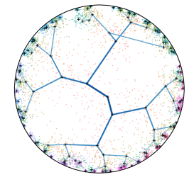
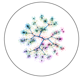
Figure 9: Branching diffusion process latent representations of $\mathcal{P}^{c}$-VAE with decreasing curvatures $c=1.2,0.3,0.1$ (Left to Right).

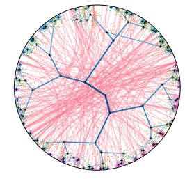
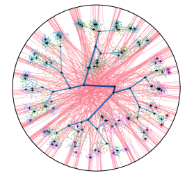
Figure 10: Branching diffusion process latent representations of $\mathcal{P}^{c}$-VAE with decreasing curvatures $c=1.2,0.3,0.1$ (Left to Right).

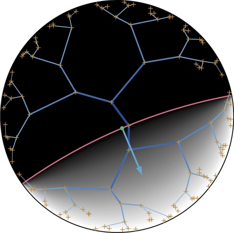
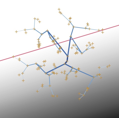
Figure 11: Branching diffusion process latent representation of $\mathcal{P}^{1}$-VAE (Left) and $\mathcal{N}$-VAE (Right) with heatmap of the log distance to the hyperplane (in pink).

References

- Beltrami, (1868) Beltrami, E. (1868). Teoria fondamentale degli spazii di curvatura costante: memoria. F. Zanetti.
- Bengio et al., (2013) Bengio, Y., Courville, A., and Vincent, P. (2013). Representation learning: A review and new perspectives. IEEE Trans. Pattern Anal. Mach. Intell., 35(8):1798–1828.
- Bonnabel, (2013) Bonnabel, S. (2013). Stochastic gradient descent on riemannian manifolds. IEEE Transactions on Automatic Control, 58(9):2217–2229.
- Box and Muller, (1958) Box, G. E. P. and Muller, M. E. (1958). A note on the generation of random normal deviates. Ann. Math. Statist., 29(2):610–611.
- Burda et al., (2015) Burda, Y., Grosse, R., and Salakhutdinov, R. (2015). Importance Weighted Autoencoders. arXiv.org.
- Chamberlain et al., (2017) Chamberlain, B. P., Clough, J., and Deisenroth, M. P. (2017). Neural Embeddings of Graphs in Hyperbolic Space. arXiv.org.
- Chevallier et al., (2015) Chevallier, E., Barbaresco, F., and Angulo, J. (2015). Probability density estimation on the hyperbolic space applied to radar processing. In Nielsen, F. and Barbaresco, F., editors, Geometric Science of Information, pages 753–761, Cham. Springer International Publishing.
- Clauset et al., (2008) Clauset, A., Moore, C., and Newman, M. E. J. (2008). Hierarchical structure and the prediction of missing links in networks. Nature, 453:98–101.
- Coates et al., (2011) Coates, A., Lee, H., and Ng, A. (2011). An analysis of single-layer networks in unsupervised feature learning. In Gordon, G., Dunson, D., and Dudík, M., editors, Proceedings of the Fourteenth International Conference on Artificial Intelligence and Statistics, volume 15 of JMLR Workshop and Conference Proceedings, pages 215–223. JMLR W&CP.
- Collins and Quillian, (1969) Collins, A. and Quillian, M. (1969). Retrieval time from semantic memory. Journal of Verbal Learning and Verbal Behavior, 8:240–248.
- Darwin, (1859) Darwin, C. (1859). On the Origin of Species by Means of Natural Selection. Murray, London. or the Preservation of Favored Races in the Struggle for Life.
- Davidson et al., (2018) Davidson, T. R., Falorsi, L., De Cao, N., Kipf, T., and Tomczak, J. M. (2018). Hyperspherical variational auto-encoders. 34th Conference on Uncertainty in Artificial Intelligence (UAI-18).
- Duda et al., (2000) Duda, R. O., Hart, P. E., and Stork, D. G. (2000). Pattern Classification (2Nd Edition). Wiley-Interscience, New York, NY, USA.
- Falorsi et al., (2018) Falorsi, L., de Haan, P., Davidson, T. R., De Cao, N., Weiler, M., Forré, P., and Cohen, T. S. (2018). Explorations in Homeomorphic Variational Auto-Encoding. arXiv e-prints, page arXiv:1807.04689.
- Figurnov et al., (2018) Figurnov, M., Mohamed, S., and Mnih, A. (2018). Implicit reparameterization gradients. In International Conference on Neural Information Processing Systems, pages 439–450.
- Ganea et al., (2018) Ganea, O.-E., Bécigneul, G., and Hofmann, T. (2018). Hyperbolic neural networks. In International Conference on Neural Information Processing Systems, pages 5350–5360.
- Ghahramani et al., (2010) Ghahramani, Z., Jordan, M. I., and Adams, R. P. (2010). Tree-structured stick breaking for hierarchical data. In Lafferty, J. D., Williams, C. K. I., Shawe-Taylor, J., Zemel, R. S., and Culotta, A., editors, Advances in Neural Information Processing Systems 23, pages 19–27. Curran Associates, Inc.
- Goh et al., (2007) Goh, K.-I., Cusick, M. E., Valle, D., Childs, B., Vidal, M., and Barabási, A.-L. (2007). The human disease network. Proceedings of the National Academy of Sciences, 104(21):8685–8690.
- Grattarola et al., (2019) Grattarola, D., Livi, L., and Alippi, C. (2019). Adversarial autoencoders with constant-curvature latent manifolds. Appl. Soft Comput., 81.
- Griffiths et al., (2004) Griffiths, T. L., Jordan, M. I., Tenenbaum, J. B., and Blei, D. M. (2004). Hierarchical topic models and the nested chinese restaurant process. In Thrun, S., Saul, L. K., and Schölkopf, B., editors, Advances in Neural Information Processing Systems 16, pages 17–24. MIT Press.
- Hauberg, (2018) Hauberg, S. (2018). Directional statistics with the spherical normal distribution. In Proceedings of 2018 21st International Conference on Information Fusion, FUSION 2018, pages 704–711. IEEE.
- Heller and Ghahramani, (2005) Heller, K. A. and Ghahramani, Z. (2005). Bayesian hierarchical clustering. In International Conference on Machine Learning, ICML ’05, pages 297–304, New York, NY, USA. ACM.
- Hofbauer et al., (2016) Hofbauer, W., Forrest, L., M. Hollingsworth, P., and Hart, M. (2016). Preliminary insights from dna barcoding into the diversity of mosses colonising modern building surfaces. Bryophyte Diversity and Evolution, 38:1.
- Hsu, (2008) Hsu, E. P. (2008). A brief introduction to brownian motion on a riemannian manifold.
- Huang and LeCun, (2006) Huang, F. J. and LeCun, Y. (2006). Large-scale learning with SVM and convolutional for generic object categorization. In CVPR (1), pages 284–291. IEEE Computer Society.
- Keil, (1979) Keil, F. (1979). Semantic and Conceptual Development: An Ontological Perspective. Cognitive science series. Harvard University Press.
- Kingma and Ba, (2016) Kingma, D. P. and Ba, J. (2016). Adam: A Method for Stochastic Optimization. In Proceedings of the International Conference on Learning Representations (ICLR).
- Kingma and Welling, (2014) Kingma, D. P. and Welling, M. (2014). Auto-encoding variational bayes. In Proceedings of the International Conference on Learning Representations (ICLR).
- Kipf and Welling, (2016) Kipf, T. N. and Welling, M. (2016). Variational graph auto-encoders. Workshop on Bayesian Deep Learning, NIPS.
- Larsen et al., (2001) Larsen, J., Szymkowiak, A., and Hansen, L. K. (2001). Probabilistic hierarchical clustering with labeled and unlabeled data.
- LeCun and Cortes, (2010) LeCun, Y. and Cortes, C. (2010). MNIST handwritten digit database.
- Ley and Verdebout, (2017) Ley, C. and Verdebout, T. (2017). Modern Directional Statistics. New York: Chapman and Hall/CRC.
- Li et al., (2019) Li, H., Lindenbaum, O., Cheng, X., and Cloninger, A. (2019). Variational Random Walk Autoencoders. arXiv.org.
- Mardia and Jupp, (2009) Mardia, K. and Jupp, P. (2009). Directional Statistics. Wiley Series in Probability and Statistics. Wiley.
- Mardia, (1975) Mardia, K. V. (1975). Statistics of directional data. Journal of the Royal Statistical Society: Series B (Methodological), 37(3):349–371.
- Nagano et al., (2019) Nagano, Y., Yamaguchi, S., Fujita, Y., and Koyama, M. (2019). A Differentiable Gaussian-like Distribution on Hyperbolic Space for Gradient-Based Learning. In International Conference on Machine Learning (ICML).
- Nickel and Kiela, (2017) Nickel, M. and Kiela, D. (2017). Poincaré embeddings for learning hierarchical representations. In Advances in Neural Information Processing Systems, pages 6341–6350.
- Nickel and Kiela, (2018) Nickel, M. and Kiela, D. (2018). Learning Continuous Hierarchies in the Lorentz Model of Hyperbolic Geometry. In International Conference on Machine Learning (ICML).
- Nooy et al., (2011) Nooy, W. D., Mrvar, A., and Batagelj, V. (2011). Exploratory Social Network Analysis with Pajek. Cambridge University Press, New York, NY, USA.
- Ovinnikov, (2018) Ovinnikov, I. (2018). Poincaré Wasserstein Autoencoder. NeurIPS Workshop on Bayesian Deep Learning, pages 1–8.
- Paeng, (2011) Paeng, S.-H. (2011). Brownian motion on manifolds with time-dependent metrics and stochastic completeness. Journal of Geometry and Physics, 61(5):940 – 946.
- Pascucci et al., (2011) Pascucci, V., Tricoche, X., Hagen, H., and Tierny, J. (2011). Topological Methods in Data Analysis and Visualization: Theory, Algorithms, and Applications. Springer Publishing Company, Incorporated, 1st edition.
- Paszke et al., (2017) Paszke, A., Gross, S., Chintala, S., Chanan, G., Yang, E., DeVito, Z., Lin, Z., Desmaison, A., Antiga, L., and Lerer, A. (2017). Automatic differentiation in pytorch. In NIPS-W.
- Pennec, (2006) Pennec, X. (2006). Intrinsic statistics on riemannian manifolds: Basic tools for geometric measurements. Journal of Mathematical Imaging and Vision, 25(1):127.
- Petersen, (2006) Petersen, P. (2006). Riemannian Geometry. Springer-Verlag New York.
- R. Gilks and Wild, (1992) R. Gilks, W. and Wild, P. (1992). Adaptive rejection sampling for gibbs sampling. 41:337–348.
- Rey et al., (2019) Rey, L. A. P., Menkovski, V., and Portegies, J. W. (2019). Diffusion Variational Autoencoders. CoRR.
- Rezende et al., (2014) Rezende, D. J., Mohamed, S., and Wierstra, D. (2014). Stochastic Backpropagation and Approximate Inference in Deep Generative Models. In International Conference on Machine Learning (ICML).
- Rossi and Ahmed, (2015) Rossi, R. A. and Ahmed, N. K. (2015). The network data repository with interactive graph analytics and visualization. In Proceedings of the Twenty-Ninth AAAI Conference on Artificial Intelligence, AAAI’15, pages 4292–4293. AAAI Press.
- Roy et al., (2006) Roy, D. M., Kemp, C., Mansinghka, V. K., and Tenenbaum, J. B. (2006). Learning annotated hierarchies from relational data. In NIPS, pages 1185–1192. MIT Press.
- Saha et al., (2018) Saha, S., Varma, G., and Jawahar, C. V. (2018). Class2str: End to end latent hierarchy learning. International Conference on Pattern Recognition (ICPR), pages 1000–1005.
- Said et al., (2014) Said, S., Bombrun, L., and Berthoumieu, Y. (2014). New riemannian priors on the univariate normal model. Entropy, 16(7):4015–4031.
- Sala et al., (2018) Sala, F., De Sa, C., Gu, A., and Re, C. (2018). Representation tradeoffs for hyperbolic embeddings. In Dy, J. and Krause, A., editors, Proceedings of the 35th International Conference on Machine Learning, volume 80 of Proceedings of Machine Learning Research, pages 4460–4469, Stockholmsmässan, Stockholm Sweden. PMLR.
- Salakhutdinov et al., (2011) Salakhutdinov, R. R., Tenenbaum, J. B., and Torralba, A. (2011). One-shot learning with a hierarchical nonparametric bayesian model. In ICML Unsupervised and Transfer Learning.
- Sanderson and Eriksson, (1994) Sanderson, M. J., M. J. D. W. P. and Eriksson, T. (1994). Treebase: a prototype database of phylogenetic analyses and an interactive tool for browsing the phylogeny of life. American Journal of Botany.
- Sarkar, (2012) Sarkar, R. (2012). Low distortion delaunay embedding of trees in hyperbolic plane. In van Kreveld, M. and Speckmann, B., editors, Graph Drawing, pages 355–366, Berlin, Heidelberg. Springer Berlin Heidelberg.
- Teh et al., (2008) Teh, Y. W., Daume III, H., and Roy, D. M. (2008). Bayesian agglomerative clustering with coalescents. In Platt, J. C., Koller, D., Singer, Y., and Roweis, S. T., editors, Advances in Neural Information Processing Systems 20, pages 1473–1480. Curran Associates, Inc.
- Tifrea et al., (2019) Tifrea, A., Becigneul, G., and Ganea, O.-E. (2019). Poincare glove: Hyperbolic word embeddings. In International Conference on Learning Representations (ICLR).
- Tolstikhin et al., (2018) Tolstikhin, I., Bousquet, O., Gelly, S., and Schoelkopf, B. (2018). Wasserstein auto-encoders. In International Conference on Learning Representations.
- Ungar, (2008) Ungar, A. A. (2008). A gyrovector space approach to hyperbolic geometry. Synthesis Lectures on Mathematics and Statistics, 1(1):1–194.