Quantum chaos transition in a two-site SYK model dual to an eternal traversable wormhole

Abstract

It has been recently proposed by Maldacena and Qi that an eternal traversable wormhole in a two dimensional Anti de Sitter space (${\rm AdS}_{2}$) is the gravity dual of the low temperature limit of two Sachdev-Ye-Kitaev (SYK) models coupled by a relevant interaction (which we will refer to as spin operator). In this paper, we study spectral and eigenstate properties of this coupled SYK model. We have found that level statistics in the tail of the spectrum, and for a sufficiently weak coupling, shows substantial deviations from random matrix theory which suggests that traversable wormholes are not quantum chaotic. By contrast, for sufficiently strong coupling, corresponding to the black hole phase, level statistics are well described by random matrix theory. This transition in level statistics coincides approximately with a previously reported Hawking-Page transition for weak coupling. We have shown explicitly that this thermodynamic transition turns into a sharp crossover as the coupling increases. Likewise, this critical coupling also corresponds with the one at which the overlap between the ground state and the thermofield double state (TFD) is smallest. In the range of sizes we can reach by exact diagonalization, the ground state is well approximated by the TFD state only in the strong coupling limit. This is due to the fact that the ground state is close to the eigenstate of the spin operator corresponding to the lowest eigenvalue which is an exact TFD state at infinite temperature. In this region, the spectral density is separated into blobs centered around the eigenvalues of the spin operator. For weaker couplings, the exponential decay of coefficients in a tensor product basis, typical of the TFD, becomes power law. Finally, we have also found that the total Hamiltonian has an additional discrete symmetry which has not been reported previously.

I Introduction

The dynamics of quantum many-body systems is very rich and, in general, highly dependent of the details of both initial conditions and the Hamiltonian that governs its time evolution. However there are situations where the time evolution has universal features. A paradigmatic example is that of a quantum system whose classical counterpart is chaotic for time scales of the order of the inverse of the mean level spacing, the so called Heisenberg time. In that region, where the discreteness of the spectrum is relevant, and therefore quantum effects are always strong, quantum chaotic systems, assuming localization effects are negligible, relax to a fully ergodic state that only depends on the global symmetries of the system. Level statistics are a powerful tool to detect and classify universal features in this region, because it is expected that the predictions of random matrix theory will apply in this case. Indeed, agreement with random matrix theory results has been found in a broad variety of systems: highly excited states of nuclei Wigner (1951), weakly disordered systems with Bertrand and García-García (2016) and without interactions Efetov (1983), deterministic quantum chaotic systems Bohigas et al. (1984) or the low energy limit of QCD in a box Verbaarschot and Zahed (1993); Shuryak and Verbaarschot (1993).

The field of quantum chaos received an important boost after it was claimed Maldacena et al. (2016a) that quantum black holes in the semiclassical limit are quantum chaotic. More specifically, it was proposed Maldacena et al. (2016a) that the growth of certain out-of-time-ordered correlation functions in the semiclassical limit, and for intermediate times of the order of the Ehrenfest time, is exponential as for quantum chaotic systems Larkin and Ovchinnikov (1969). Moreover, the growth rate, given by the Lyapunov exponent, obeys a universal bound which is saturated for field theories with a gravity dual. Later this feature was also observed Kitaev ; Maldacena and Stanford (2016) in the strong coupling limit of the Sachdev-Ye-Kitaev (SYK) model Bohigas and Flores (1971a, b); French and Wong (1970, 1971); Mon and French (1975); Benet and Weidenmüller (2003); Kota (2014); Sachdev and Ye (1993); Sachdev (2010); Kitaev ; Fu et al. (2017), a zero dimensional fermionic model with infinite-range random interactions. This simple quantum mechanical model has attracted a great deal of attention because, despite being quantum chaotic and strongly interacting, it can be tackled analytically Kitaev ; Maldacena and Stanford (2016); García-García and Verbaarschot (2017); Stanford and Witten (2017); Mertens et al. (2017); Belokurov and Shavgulidze (2017); Bagrets et al. (2016, 2017); Jevicki et al. (2016); Aref ’eva et al. (2018); Altland and Bagrets (2018) and has all the features expected for a system with a gravity dual Kitaev ; Maldacena and Stanford (2016); Jensen (2016); Jevicki et al. (2016): it does saturate the bound on chaos mentioned above, it also has a finite zero temperature entropy Sachdev and Ye (1993), a linear specific heat in the low temperature limit Kitaev ; Maldacena and Stanford (2016); García-García and Verbaarschot (2017); Cotler et al. (2017) and a density of low energy excitations Maldacena and Stanford (2016); Cotler et al. (2017); García-García and Verbaarschot (2017) that increases exponentially. Level statistics of the SYK model was shown to be well described by random matrix theory García-García and Verbaarschot (2016); Cotler et al. (2017); García-García and Verbaarschot (2017); Altland and Bagrets (2018); García-García et al. (2018) in the spectral region where the SYK model is expected to have a gravity dual which confirms that it is also quantum chaotic for long times. Based on the same pattern of conformal symmetry breaking, Maldacena et al. (2016b); Almheiri and Polchinski (2015), the gravity dual of the SYK model has been identified to be a Jackiw-Teitelboim Jackiw (1985); Teitelboim (1983); Förste and Golla (2017) background.

A natural question to ask, assuming that the holographic duality applies for sufficiently long times, is whether these quantum chaotic features are exclusive to quantum black holes geometries, such as the Jackiw-Teitelboim background, or also apply to other backgrounds. Recently, Maldacena and Qi Maldacena and Qi (2018), see also Bak et al. (2018); Kim et al. (2019), constructed a near ${\rm AdS}_{2}$ background representing an eternal traversable wormhole. The quantum feasibility of a traversable wormhole was previously suggested Gao et al. (2017) by showing that a double trace deformation could make the quantum matter stress tensor to have a negative average null energy without violating causality. An example of such construction for ${\rm AdS}_{2}$ geometries was worked out in Maldacena et al. (2017) and for higher dimensions, and other backgrounds, in Fu et al. (2018); Tumurtushaa and Yeom (2018); Maldacena et al. (2018); Anabalón and Oliva (2018) Out of equilibrium features for intermediate times were investigated in Ref. Gao and Liu (2018) and entanglement and other quantum information observables were studied in Ref. Bao et al. (2018).

Returning to eternal traversable wormholes, it was conjectured Maldacena and Qi (2018) that its ground state is well approximated by a thermofield double state (TFD) and that its field theory dual is a two-site SYK model coupled by a relevant interaction in the limit of weak coupling and low temperature. It was found that for sufficiently high temperatures, or stronger coupling, the system undergoes a thermodynamic Hawking-Page transition from the wormhole phase to a two black hole phase. By increasing the strength of the coupling, the transition takes place at higher temperatures and finally, after reaching the critical coupling, this first order transition terminates. Intriguingly, the wormhole phase is still controlled by a generalized Schwarzian action when the residual SL($2$) symmetry of the standard SYK model is broken Maldacena and Qi (2018). The associated Liouville quantum mechanics problem Bagrets et al. (2016) has graviton bound states which are interpreted as excited states of the quantum wormhole background. A non-random SYK model with the same large $N$ limit was investigated previously in Ref. Azeyanagi et al. (2018) with similar conclusions.

In this paper, we study different aspects of this coupled SYK model. Our motivation is twofold. First, we aim to investigate the long time dynamics of this two-site coupled SYK model by level statistics in order to clarify whether quantum chaos and random matrix theory are generic in quantum gravity backgrounds or are restricted to black holes. Second, we would like to gain a more detailed understanding of the phase diagram of the system. More specifically, we aim to determine the range of validity of the TFD as a ground state of the system and also the exact nature of the termination of the first order Hawking-Page transition at finite coupling. We have found that indeed these two main goals are closely related. We show that the first order transition suddenly becomes a sharp crossover above the critical coupling. Around the same coupling strength, the number of non-zero coefficients, in a tensor product basis of the two independent SYK’s, that contribute substantially to the ground state of the system increases sharply. This is typical of chaotic-integrable transitions. More specifically, except for strong coupling and in the range of sizes we can explore numerically, we have observed that the energy dependence of these coefficients is power law rather than the exponential decay typical of the TFD state.

Level statistics are also sensitive to the value of the coupling constant. In the tail of the spectrum, and couplings weaker than the critical one, corresponding to the wormhole phase, level statistics are not described by random matrix theory. However, well above the critical coupling, spectral correlations in the full spectrum are well described by random matrix theory.

The organization of the paper is as follows. First, we introduce the model with a special emphasis on the description of its symmetries and its ground state. In particular, we identify a global spin symmetry in the combined system that has an important effect on spectral statistics and thermodynamic properties. In Section III, we investigate the ground state of the system. For the number of Majoranas we can simulate by exact diagonalization, the ground state is well approximated by TFD only in the limit of strong coupling between the two SYK’s. Thermodynamic properties are investigated in Section IV. We have found that the first order transition at a finite coupling, reported in Ref. Maldacena and Qi (2018), is followed by a sharp crossover for stronger coupling. At the critical coupling the overlap between the ground state and TFD is smallest. In the strong coupling limit, the spectral density develops well separated blobs centered around the spin eigenvalues that control the free energy. Section V is devoted to the analysis of level statistics. For weak coupling, and in the infrared region of the spectrum, corresponding to the traversable wormhole phase, we did not find agreement with the random matrix theory, thus suggesting that the gravitational bound states in this phase are not quantum chaotic. However, for sufficiently large coupling, corresponding to the black hole phase, level statistics are well described by random matrix theory. Finally, in Section VI, devoted to outlook and conclusions, we speculate that the termination of the observed transition at strong coupling is reminiscent of a Gross-Witten transition Gross and Witten (1980a), induced by the gradual reduction of the effect of interactions by increasing the coupling between the two SYK models.

II The model and its symmetries

We study $N$ Majorana fermions in $(0+1)$ dimensions where the first $N/2$ fermions, $\psi_{L}$, are labeled by Left ($L$), and the remaining $N/2$, labeled by $R$, $\psi_{R}$, will be called the Right ($R$) fermions. In each of these two subspaces, the dynamics is governed by the SYK model,

$$H_{L}\, =\,\frac{1}{4!}\sum_{i,j,k,l=1}^{N/2}J_{ijkl}\,\psi_{L,i}\,\psi_{L,j}\,\psi_{L,k}\,\psi_{L,l}\,$$

$$H_{R}\, =\,\frac{1}{4!}\sum_{i,j,k,l=1}^{N/2}J_{ijkl}\,\psi_{R,i}\,\psi_{R,j}\,\psi_{R,k}\,\psi_{R,l}$$ (1)

where $\psi_{L,i},\psi_{R,i}$ are Majorana fermions $\{\psi_{A,i},\psi_{B,j}\}=\delta_{AB}\delta_{ij}$ $(A,B=L,R)$ and $J_{ijkl}$ are Gaussian distributed random variables with $\langle J_{ijkl}\rangle=0$ and standard deviation $\langle J_{ijkl}^{2}\rangle=4\sqrt{6}J/{N^{3/2}}$ Kitaev ; Maldacena and Stanford (2016).

The two SYK model are coupled by the following interaction:

$$H_{\rm int}=ik\sum_{j=1}^{N/2}\psi_{L,j}\psi_{R,j},$$ (2)

so that the total Hamiltonian is simply given by,

$$H_{\rm total}=H_{L}+\alpha H_{R}+H_{\rm int}$$ (3)

For the moment we set $\alpha=1$ in which case the Hamiltonian has an extra global spin symmetry that we will discuss in detail shortly. For the study of level statistics we will find it computationally advantageous to break this symmetry by setting $\alpha\neq 1$ to a slightly different value which does not affect qualitatively most of the key features of the model Maldacena and Qi (2018), like for example the observed gap between the ground state and the first excited state.

The anti-commutation relations of $\psi_{L,i},\psi_{R,i}$ can be realized by introducing $N$ Gamma matrices $\Gamma_{i}$ as

$$\psi_{L,i}=\frac{1}{\sqrt{2}}\Gamma_{i},\quad\psi_{R,i}=\frac{1}{\sqrt{2}}\Gamma_{{N}/{2}+i}.$$ (4)

Since each term in the full Hamiltonian is an even power of the Gamma matrices, the full Hamiltonian preserves chirality, defined as the eigenvalue of $\Gamma_{c}=\Gamma_{1}\Gamma_{2}\cdots\Gamma_{N}$. We have summarized the notation for the Gamma matrices and related symmetries in appendix A.

II.1 $S$ mod 4 symmetry

Let us define the spin operator $S$ as

$$S=i\sum_{j=1}^{{N}/{2}}\psi_{L,j}\psi_{R,j}=\frac{i}{2}\sum_{i=1}^{{N}/{2}}\Gamma_{j}\Gamma_{{N}/{2}+j},$$ (5)

that is, $H_{\rm int}=kS$. Below we show that $S$ has the discrete spectrum $S=-N/4,-N/4+1,\cdots,N/4$ and that, if $\alpha=1$, the full Hamiltonian (3) preserves $S$ mod 4 in addition to the chirality ($S$ mod 2). We shall call $S$ the spin operator.

First, let us deduce the spectrum of $S$. If we define $\Gamma^{\pm}_{i}$ as

$$\Gamma^{\pm}_{i}=\Gamma_{{N}/{2}+i}\pm i\Gamma_{i},$$ (6)

then $S$ can be written as

$$S=\frac{1}{4}\sum_{i=1}^{{N}/{2}}\Gamma^{+}_{i}\Gamma^{-}_{i}-\frac{N}{4}.$$ (7)

The operators $\Gamma^{\pm}_{i}$ also satisfy the following (anti)commutation relations

$$\{\Gamma^{\pm}_{i},\Gamma^{\pm^{\prime}}_{j}\} =0\quad(i\neq j),\quad\Gamma^{\pm}_{i}\Gamma^{\pm}_{i}=0\quad\text{(with no contraction)}$$

$$[S,\Gamma^{\pm}_{i}] =\pm\Gamma^{\pm}_{i},$$ (8)

from which we can derive the following spectrum:

(17)

where $|S=-N/4\rangle$ is the lowest spin state satisfying

$$\Gamma^{-}_{i}|S=-N/4\rangle=0.$$ (18)

Next we discuss the $S$ mod 4 symmetry. If we define

$$P_{ij} =2(\psi_{L,i}\psi_{L,j}+\psi_{R,i}\psi_{R,j})=\Gamma_{i}\Gamma_{j}+\Gamma_{N/2+i}\Gamma_{N/2+j},$$

$$Q_{ij} =2(\psi_{L,i}\psi_{L,j}-\psi_{R,i}\psi_{R,j})=\Gamma_{i}\Gamma_{j}-\Gamma_{N/2+i}\Gamma_{N/2+j},$$ (19)

the full Hamiltonian (3) with $\alpha=1$ can be written as

$$H=\frac{1}{8}\sum_{i<j<k<l}^{N/2}J_{ijkl}(P_{ij}P_{kl}+Q_{ij}Q_{kl})+kS.$$ (20)

The $P_{ij}$ and $Q_{ij}$ operators satisfy the following commutation relations with $S$

$$[S,P_{ij}]=0,\quad[S,[S,Q_{ij}]]-4Q_{ij}=0.$$ (21)

That is, $P_{ij}$ preserves the spin $S$. To interpret the commutation relation for $Q_{ij}$ it is convenient to act Eq. (21) on an eigenstate of $S$, with the spin eigenvalue $s$, which we shall call $|\phi\rangle$. One easily derives

$$(S^{2}-2sS+s^{2}-4)Q_{ij}|\phi\rangle=0.$$ (22)

This implies that an expansion of $Q_{ij}|\phi\rangle$ contains only spin eigenstates with $S=s\pm 2$. Hence $S$ mod 4 is a symmetry of $Q_{ij}Q_{k\ell}$. Putting the above computations together we find that the full Hamiltonian Eq. (3) preserves also the $S$ mod 4 symmetry.

It is instructive to express the exponent of the spin operator as a product

$$e^{i\theta S}=\prod_{i=1}^{N/2}\left(\cos\frac{\theta}{2}-\sin\frac{\theta}{2}\Gamma_{i}\Gamma_{N/2+i}\right).$$ (23)

For $\theta=\pi$ we recover the chirality operator, while $\theta=\pi/2$ gives the $S$ mod 4 symmetry,

$$[e^{\pi iS/2},H]=0.$$ (24)

This also shows that the chirality symmetry operator is the square of the $S$ mod 4 operator. In appendix B, we give an alternative proof of the $S$ mod 4 symmetry based on the product form Eq. (23).

This $S$ mod 4 symmetry plays an important role when we analyze the level correlations. For $\alpha=1$, the full Hamiltonian splits into four blocks labeled by $S$ mod 4, regardless of the value of the random coupling $J_{ijkl}$. When analyzing level correlations, unitary symmetries have to be taken into account exactly and we have to focus on a single block. We revisit this issue in section V. For $\alpha\neq 1$, the full Hamiltonian only preserves chirality and there is no $S$ mod 4 symmetry.

III Comparison of the TFD state with ground state

Here we consider the case with identical L and R systems, i.e. $\alpha=1$. For $k=0$ (and $N=0$ mod 4 so that $N/2$ is even), the system we are considering is $H=H_{SYK}\otimes 1+1\otimes H_{SYK}$. That is, the system consists of two decoupled SYK systems with $N/2$ fermions, the L and R systems, which are identical to each other. It was already pointed out in Maldacena and Qi (2018) that when the interaction between L-system and R-system is turned on the ground state has a large overlap with the Thermo Field Double (TFD) state of $H_{SYK}\otimes 1+1\otimes H_{SYK}$. In this section, we shall study this similarity in more detail.

Because the left and right systems are identical, the left and right $\Gamma$-matrices can be represented as

$$\Gamma_{k}^{L} = \gamma_{k}\otimes 1,$$

$$\Gamma^{R}_{k} = \gamma_{c}\otimes U\gamma_{k}U^{-1},$$ (25)

where $U$ is a unitary matrix (we use the notation that the lower case gamma matrices are of size $2^{N/4}\times 2^{N/4}$ and upper case gamma matrices are of size $2^{N/4}\times 2^{N/4}$).

The factor $\gamma_{c}$ ensures that the left $\Gamma$ matrices anti-commute with the right $\Gamma$ matrices. Below, we will call this basis the tensor basis. If the eigenvalues and eigenstates of $H_{L}$ are given by

$$H_{L}|n\rangle_{L}=E_{n}|n\rangle_{L},$$ (26)

then

$$H_{R}|n\rangle_{R}=E_{n}U|n\rangle_{R},\;\text{with}\;|n\rangle_{R}=U|n\rangle_{L}.$$ (27)

Let us define the TFD state,

$$|{\rm TFD}\rangle=\sum_{n}e^{-2\beta\,E_{n}+i\phi_{n}}|n\rangle_{L}e^{i\frac{\pi}{4}\gamma_{c}}CK|n\rangle_{R},$$ (28)

where we have included a phase factor, $\exp i\phi_{n}$ and $CK$ is the charge conjugation operator. We will next show that

$$|I\rangle\equiv|S=-N/4\rangle=\sum_{n}|n\rangle_{L}\otimes e^{i\frac{\pi}{4}\gamma_{c}}CK|n\rangle_{R}$$ (29)

is the ground state of the spin operator. To this end we calculate the expectation value

$$\langle I|S|I\rangle = 2^{-N/4}\sum_{n,m}\Bigl{(}\langle n|_{L}\otimes\langle e^{i\frac{\pi}{4}\gamma_{c}}CKn|_{R}\Bigr{)}S\Bigl{(}|m\rangle_{L}\otimes e^{i\frac{\pi}{4}\gamma_{c}}CK|m\rangle_{R}\Bigr{)}$$ (30)

$$= 2^{-N/4}\frac{i}{2}\sum_{n,m}\sum_{k}\langle n|_{L}\gamma_{k}\gamma_{c}|m\rangle_{L}\langle e^{i\frac{\pi}{4}\gamma_{c}}CKn|_{R}\gamma_{k}e^{i\frac{\pi}{4}\gamma_{c}}CK|m\rangle_{R}$$

$$= 2^{-N/4}i\sum_{n,m}\sum_{k}\chi_{m}\langle n|_{L}\gamma_{k}|m\rangle_{L}\frac{i}{2}\chi_{m}\langle m|_{R}\gamma_{k}|n\rangle_{R},$$

where $\chi_{m}$ is the chirality of the state $|m\rangle$,

$$\gamma_{c}|m\rangle=\chi_{m}|m\rangle.$$ (31)

Choosing $|m\rangle_{R}=|m\rangle_{L}$ (i.e. $U=1$ in Eq. (25)) the sum over $m$ can be eliminated by completeness.

r.h.s. of Eq. (30) $$= -2^{-N/4}\frac{1}{2}\sum_{n}\sum_{k}\langle n|_{R}\gamma_{k}^{2}|n\rangle_{R}$$ (32)

$$= -\frac{N}{4},$$

which is the desired result. Therefore $|I\rangle$ is the state with the lowest spin. A similar prove can be used to show that $\|\Gamma_{i}^{-}|S=-N/4\rangle\|^{2}=0$ (no sum over $i$). This shows that the state $|I\rangle$ is annihilated by all lowering operators ${\Gamma^{-}}_{i}$. The details of the ground state which depend on $N/2\mod 8$ are worked out in Appendix D for $N/2\mod 8=4$, in Appendix C for $N/2\mod 8=2$ and in Appendix E for $N/2\mod 8=0$.

At finite temperature, we define the TFD state $|\text{TFD}\rangle_{\beta}$ as

$$|TFD\rangle_{\beta}=\frac{1}{\sqrt{Z(N,\beta)}}e^{-\beta(H_{SYK}\otimes 1+1\otimes H_{SYK})}|S=-N/4\rangle,$$ (33)

where $Z(N,\beta)$ is a normalization factor such that $\langle\text{TFD}|_{\beta}\text{TFD}\rangle_{\beta}=1$. As confirmed by numerical calculations for $N$ up to 32, the complex phase factor of the $|n\rangle\otimes|n\rangle$ components of the ground state at finite coupling $k$, does not depend on $k$. This is a nontrivial result which we only understand perturbatively.

III.1 $|\text{TFD}\rangle_{\beta}$ versus ground state of coupled SYK

In Maldacena and Qi (2018) it has been argued that the ground state $|\text{gs}\rangle$ of the coupled system at finite coupling $k$ is close to the TFD state $|\text{TFD}\rangle_{\beta}$ by studying the overlap $\langle\text{TFD}|_{\beta}\text{gs}\rangle$. Here the inverse temperature $\beta$ is a function of $k$ determined by maximizing the overlap. However, it should be stressed that a large value of this overlap does not necessarily imply that the coefficients $(\langle n|\otimes\langle n|)|\text{gs}\rangle$, taken as a function of the energy levels of the single SYK system, behave like $e^{-2\beta E_{n}}$. The reason is that for small coupling most of the strength of the wave function can be localized in one or few components of the wave function. In this section we will show numerically that, at finite $N\leq 28$, this is actually the case and that for sufficiently small values of the coupling $k$ the coefficients display large deviations from the exponential behavior typical of the TFD state.

Before moving to a detailed analysis, let us first consider the results in some limiting cases. In the limit $k\rightarrow\infty$, since $H$ is dominated by $H_{int}=kS$, the ground state $|gs\rangle$ coincides with $|\text{TFD}\rangle_{\beta=0}$, see Eqs. (30), (32) and (33). In the limit $k\rightarrow 0$, on the other hand, the tensor product states $|m_{\pm}\rangle_{L}\otimes|n_{\pm^{\prime}}\rangle_{R}$ are the exact eigenstates of $H$ with the eigenvalues $E_{m}+E_{n}$, where the $E_{n}$ are the eigenvalues of a single SYK, $H_{SYK}|n_{\chi}\rangle_{L,R}=E_{n}|n_{\chi}\rangle_{L,R}$, and the index $\chi=\pm$ denotes the chirality of the state. The ground state is $|1_{\chi}\rangle_{L}\otimes|1_{\chi^{\prime}}\rangle_{R}$ which may be degenerate depending on the value of $N$. Hence the ground state in the $k\rightarrow 0$ limit is given by the $|\text{TFD}\rangle$ state for $\beta=\infty$. Note that this does not necessarily imply that the ground state is close to a TFD state for small but nonzero $k$.

Let us compare the ground state of the Hamiltonian Eq. (3) with the TFD state at finite temperature $|\text{TFD}\rangle_{\beta}$ for varying $k$. It can be expanded in the complete set $|m\rangle\otimes|n\rangle$

$$|{\rm gs}\rangle=\sum_{n}c_{n}|n\rangle\otimes|n\rangle+\sum_{m\neq n}b_{mn}|m\rangle\otimes|n\rangle.$$ (34)

Numerically, the phases of the $c_{n}$ do not depend on the coupling constant and are thus given by the phases of the ground state of $S$ (perturbed by a $\epsilon(H_{L}+H_{R})$ with $\epsilon$ a small constant). This is not the case for the phases of the coefficients $b_{mn}$. We can understand this fact to first order in perturbation theory in $1/k$ with $S$ as the zeroth order Hamiltonian,

$$|{\rm gs}\rangle=|I\rangle+\sum_{m}|S_{m}\rangle\frac{\langle S_{m}|(H_{L}+H_{R})|I\rangle}{S_{0}-S_{m}}$$ (35)

with $|S_{m}\rangle$ an eigenstate of $S$ with eigenvalue $S_{m}$ and $S_{0}$ the spin of the ground state. Inserting a complete set of eigenstates of $H_{L}+H_{R}$, $\sum_{m,n}|m\rangle\otimes|n\rangle\langle m|\otimes\langle n|$, and noticing that $\Bigl{(}\langle m|\otimes\langle n|\Bigr{)}(H_{L}+H_{R})|I\rangle=0$ for $m\neq n$, the matrix element can be written as

$$\langle S_{m}|(H_{L}+H_{R})|I\rangle=\sum_{n}\langle S_{m}|\Bigl{(}|n\rangle\otimes|n\rangle\Bigr{)}\Bigl{(}\langle n|\otimes\langle n|\Bigr{)}(H_{L}+H_{R})|I\rangle.$$ (36)

Only those states with the same $S$ mod 4 spin as the ground state contribute to the sum over $n$. It turns out that the complex phase of the matrix elements $\langle S_{m}|\Bigl{(}|n\rangle\otimes|n\rangle\Bigr{)}$ does not depend on $m$ apart from an overall phase which cancels with the contribution to the matrix element

$$\langle S_{m}|\Bigl{(}|n\rangle\otimes|n\rangle\Bigr{)}\Bigl{(}\langle n|\otimes\langle n|\Bigr{)}(H_{L}+H_{R})|I\rangle=2\langle S_{m}|\Bigl{(}|n\rangle\otimes|n\rangle\Bigr{)}E_{n}\Bigl{(}\langle n|\otimes\langle n|\Bigr{)}|I\rangle,$$ (37)

which is therefore real. The complex phase of the first order correction is therefore due to the phase of $\Bigl{(}\langle n|\otimes\langle n|\Big{)}|S_{m}\rangle$ which is the same as the phase of $\Bigl{(}\langle n|\otimes\langle n|\Bigr{)}|I\rangle$ (up to a minus sign). The same argument cannot be made for third and higher order perturbative corrections because off-diagonal states, $|m\rangle\otimes|n\rangle$ (with $m\neq n$) contribute to the intermediate state sums. We conclude that at first and second order in perturbation theory the complex phase of the ground state does not depend on $k$, up to a value of $k$ for which the perturbative contributions are larger than the $|n\rangle\otimes|n\rangle$ components of the ground state. At that point one or more components of the ground state change sign.

In the numerical studies below we will only consider the cases $N=20$ and $N=28$, where $|\text{TFD}\rangle_{\beta}$ is defined as, see Eq. (33),

$$|\text{TFD}\rangle_{\beta}=\frac{1}{\sqrt{Z(\beta)}}\sum_{n=1}^{2^{N/4-1}}e^{-2\beta E_{n}}(|n_{+}\rangle_{L}\otimes|n_{-}\rangle_{R}+|n_{-}\rangle_{L}\otimes|n_{+}\rangle_{R})\ ,$$ (38)

and $Z(\beta)=2\sum_{n=1}^{2^{N/4-1}}e^{-4\beta E_{n}}$ is the normalization factor.

Since $k$ is the parameter of the Hamiltonian that interpolates between a ground state $|\text{TFD}\rangle_{\beta=\infty}$ and $|\text{TFD}\rangle_{\beta=0}$ which also corresponds to the ground state of the spin operator, we expect that the effective inverse temperature $\beta(k)$ monotonically decreases as $k$ increases. Furthermore, we have computed $|\langle S=-N/4|gs\rangle|^{2}$ and found that this overlap is almost 1 already around $k\sim 1$ (see Fig. 1).

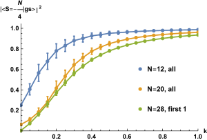
Figure 1: Overlap between the ground state of the spin operator and the ground state of the coupled SYK model as a function of the coupling $k$. Here the results for $N=12$ and $N=20$ are obtained by diagonalizing the full Hamiltonian and then extracting the eigenvector with the lowest energy eigenvalue, while for $N=28$ we have obtained only the ground state eigenvector by applying the so called Arnoldi method to the Hamiltonian shifted by a constant matrix $H-\text{diag}(100,100,\cdots,100)$. Here the shift is required technically so that the eigenvalue of the ground state has the largest absolute value among the full spectrum. Only for large $k$ is the ground state of the spin operator a good description of the ground state of the coupled SYK model.

Hence we expect the effective temperature changes substantially only in the regime $0<k<1$.

Below, to be self-contained, we first redo the comparison of the ground state and the TFD state by maximization of their overlap. This computation was already performed in Maldacena and Qi (2018). We have checked numerically, for $N=20$ and $N=28$, that the maximized overlap with respect to $\beta$, between the TFD state and the ground state, is close to $1$. For this purpose, we have considered the ansatz Eq. (38) for the ground state, in which the $E_{n}$ are the energy levels of a single SYK model and $\beta$ is the fitting parameter determined by maximizing the overlap. We normalize this state as $\langle\text{TFD}|_{\beta}\text{TFD}\rangle_{\beta}=1$ by choosing $Z(\beta)$ as

$$Z(\beta) =2\sum_{n=1}^{2^{N/4-1}}e^{-4\beta E_{n}}\ ,$$ (39)

which therefore has not been considered as an independent fitting parameter. We proceed as follows:

1. Generate an ensemble of $2^{N/4}\times 2^{N/4}$ matrices $H_{SYK}=\frac{1}{2}\sum_{i<j<k<\ell}J_{ijk\ell}\gamma_{i}\gamma_{j}\gamma_{k}\gamma_{\ell}$ with Gaussian random $J_{ijk\ell}$, and compute their eigenvalues $\{E_{n}\}$ and eigenvectors $\{|n_{\pm}\rangle\}$ through exact numerical diagonalization. Then construct the tensor product $|n_{\pm}\rangle_{L}\otimes|n_{\mp}\rangle_{R}$.

2. For the same ensemble of random couplings, generate $2^{N/2}\times 2^{N/2}$ matrices representing the Hamiltonian Eq. (3) with $\alpha=1$ using the tensor basis (25) and compute the ground state $|\text{gs}\rangle$ through the exact diagonalization.

3. Compute $c^{\pm}_{n}=(\langle n_{\pm}|_{L}\otimes\langle n_{\mp}|_{R})|{\rm gs}\rangle$. We have observed that $c^{+}_{n}=c^{-}_{n}$ and $c^{+}_{n}>0$ for all $n=1,2,\cdots 2^{N/4}/2$, up to an overall phase provided that we define the phase of $|n_{\pm}\rangle_{L,R}$ such that Eq. (38) holds without any extra phase (see appendix D for detail). Hence we shall denote $c^{+}_{n}=c^{-}_{n}$ simply by $c_{n}$.

4. For each ensemble realization determine $\beta$ by maximizing the overlap $\langle\text{TFD}|_{\beta}\text{gs}\rangle$.

   $$\langle\text{TFD}|_{\beta}\text{gs}\rangle=\frac{2}{\sqrt{Z(\beta)}}\sum_{n=1}^{2^{N/4-1}}c_{n}e^{-2\beta E_{n}}$$ (40)

5. Take average of both $\beta$ and $\langle\text{TFD}|_{\beta}\text{gs}\rangle$ over the ensemble.

Following this procedure we obtained both the effective inverse temperature $\beta(k)$ and the overlap $\langle\text{TFD}|_{\beta}\text{gs}\rangle$. The results are displayed in Fig. 2.

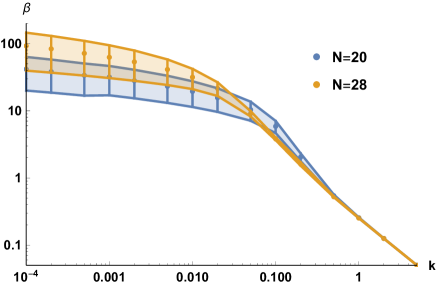
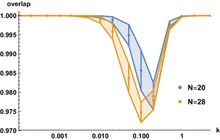
Figure 2: Left: inverse temperature $\beta$ as a function of the coupling $k$. Right: overlap $\langle\text{TFD}|_{\beta}\text{gs}\rangle$ as a function of $k$.

As we can see, the inverse temperature is indeed growing for small $k$ and it tends to zero at strong coupling as expected. In agreement with Maldacena and Qi (2018), we confirm that $\langle\text{TFD}|_{\beta}\text{gs}\rangle$ is pretty close to $1$ with relatively large deviations around $k\sim 0.1$. More quantitatively, for small $k$, the inverse effective temperature depends on $k$ roughly as $1/k^{1/6}$ while at $k\approx 0.1$, there is a transition to a $1/k$ dependence.

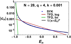
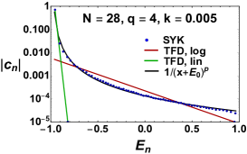
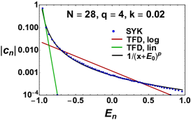
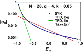
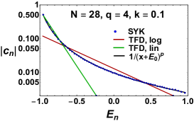
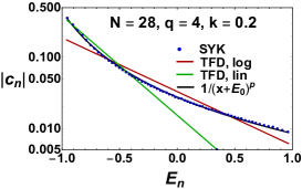
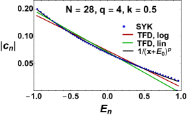
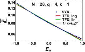
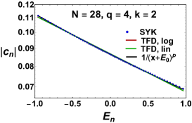
Figure 3: The agreement between the average ground state coefficients $c_{n}$ (black points) and the TFD obtained by fitting the $|c_{n}|$ configuration by configuration (green curve), or by fitting to the logarithm of the ensemble average of the $|c_{n}|$ (red and black curves). The power law ansatz (black curve) gives much better fit especially for small $k$. Note that the green curve has one fitting parameter ($\beta$), while the red (exponential) and black (power law) curves are two-paramter fits, $c$ and $\beta$ with $c$ the normalization constant, and $c$ and $e_{0}$, repectively. The value of the power in the latter case is $p=2.178$.

As was already mentioned, the large overlap between the ground state and the TFD, does not necessarily imply that the coefficients $c_{n}$ have an exponential behavior in energy. Indeed, it could be simply that one or a few coefficients in (34) are much larger than the others. In this case, the overlap $\langle\text{TFD}|_{\beta}\text{gs}\rangle$ would be very close to be $1$, even though all the other coefficients could behave in a completely different way.

Hence, to check whether the coefficients of the ground state have an exponential profile, we have studied their average on a logarithmic scale versus the ensemble average of each of the $E_{n}$ (for the case $N=28$ only). Results, depicted in Fig. 3, clearly show that an exponential form is not a good fit to the $|c_{n}|$ coefficients. For comparison, we have also included the coefficients of the TFD state with $\beta$ determined by maximizing the overlap (green curves) as described before, and fitting the logarithm of the ensemble average of $|c_{n}|$ to the TFD form also leaving the normalization constant as a free parameter (red curve). None of these fitting to the TFD state give good results. By contrast, a power law ansatz (black line),

$$c_{n}\sim\frac{c}{(E_{n}-e_{0})^{p}},$$ (41)

provides an excellent fitting. In order to compare the two parameter fits, we fix $p$ at $p=2.178$. The fitted value of $e_{0}$ is somewhat smaller than the ground state energy $E_{1}$ for small $k$ and decreasing for increasing values of $k$. The value of $c$ is in principle determined by the normalization, but leaving it as a free parameter gives a better fit. For small coupling $k<0.5$ the value of $c$ is quite different from the one obtained from the normalization. The reason is that most of the strength of the wave function is in $c_{1}$ which does not contribute much to the $\chi^{2}$ when you fit the logarithm of the $|c_{n}|$. One could also take $p$ as a $k$-dependent fitting parameter which gives slightly better fits. In any case, except in the regime of strong coupling, power law fits provide a much better description of the numerical results than exponential fits related to the TFD state. For $k\geq 1$ the TFD ansatz is a good description of the ground state though. This is consistent with the expectation that at large coupling the system is dominated by the spin operator and the TFD state (with $\beta\to 0$) is the ground state of the Hamiltonian Eq. (3).

For $k>0.2$ the energy dependence of the coefficients can also be described by the sum of two exponentials with a $\chi^{2}$ that is comparable to the power law fit, but it has one more parameter. A Gaussian dependence, $\exp(-\beta x-\alpha x^{2})$, first introduced in the context of a nuclear many body system Verbaarschot and Brussaard (1979), also gives a reasonable fit in this parameter region.

Once again, we stress that the deviation from the TFD form is not in contradiction with the good overlap between the TFD and the ground state, since the dominant coefficients are well reproduced by the TFD at least for small $k$, as it can be seen from Fig. 3.

These numerical results suggest that the coefficients of the ground state are not well approximated by the TFD ansatz, and that instead they are very close to a power law ansatz. However, we should note that $N=28$ may not be close to the large $N$ limit of this system where analytical arguments Maldacena and Qi (2018), show that the ground state is well approximated by a TFD state. This indicates that the convergence to the large $N$ limit is slow and most likely nonuniform. Interestingly, it has been observed in Cottrell et al. (2018), that the Hamiltonian Eq. (3) is just an approximation of a Hamiltonian whose exact ground state is the TFD.

In Fig. 4 we show the ratio $|c_{2}/c_{1}|$ (left) and the inverse participation ratio (IPR) (right) defined as

$${\rm IPR}=\frac{(\sum_{n}|c_{n}|^{2})^{2}}{\sum_{n}|c_{n}|^{4}}.$$ (42)

We observe a crossover at $k\approx 0.1$ where $\beta(k)\approx E_{2}-E_{1}$. Around the same value of $k$, the inverse participation ratio increases dramatically. This is a feature typical in metal-insulator and integrable-chaotic transitions.

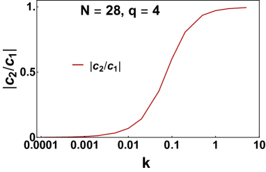
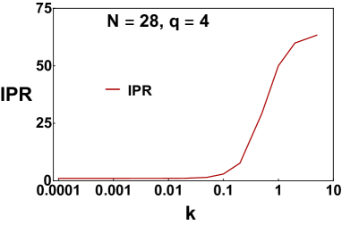
Figure 4: The ratio of $|c_{2}/c_{1}|$ (left) and the inverse participation ratio (right) versus $k$.

The results of this section suggest that the ground state of the model undergoes a qualitative change around $k\sim 0.1-0.2$. We shall see in next section that precisely in this region the first order transition mentioned in the introduction turns into a sharp crossover. We turn now to the study of low energy excitations by the analysis of thermodynamic properties and spectral correlations.

IV Thermodynamic properties

In the first subsection, we study thermodynamic properties of Hamiltonian Eq. (3) for $\alpha=1$ and $N\leq 34$ by exact diagonalization techniques. In the second subsection, we repeat this analysis in the large $N$ limit by solving the Schwinger-Dyson equations to study the Hawking-Page phase transition, first reported in Ref. Maldacena and Qi (2018), in more detail.

IV.1 Numerical Study

In order to investigate the thermodynamic properties of the Hamiltonian Eq. (3), we compute its spectrum by exact diagonalization techniques for up to $N=34$ Majoranas. We are mostly interested in the low temperature limit where, according to the results of Ref. Maldacena and Qi (2018), a first order Hawking-Page transition occurs at a finite value of the coupling $k$. The transition, according to Ref. Maldacena and Qi (2018), seems to terminate for $k\geq k_{c}$ though it is not clear whether it becomes second order or just a crossover.

We study the free energy as a function of $k$ and $N$. For any $N\gg 1$ we have found, see Fig. 5, that for sufficiently large $k$ and low temperature, the free energy, computed in the chiral sector containing the ground state, is constant which signals the existence of a gap in the spectrum, one of the distinctive features of the AdS graviton gas. Interestingly, unlike the standard SYK model, the chirality of the ground state depends on $N$, namely, for $N=26$ it is positive but for $N=28$ and $N=30$ it is negative. We do not have a clear understanding of this feature.

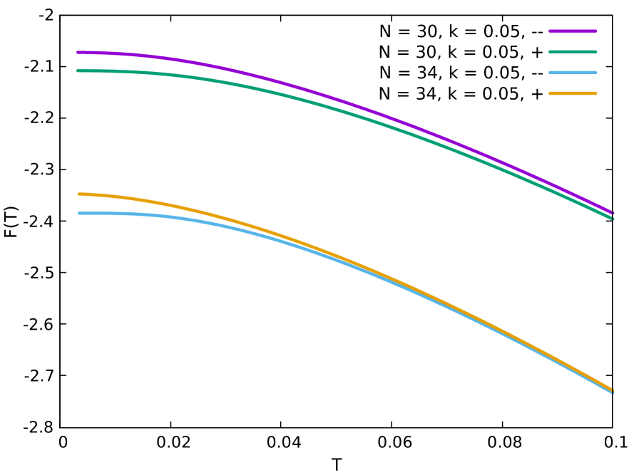
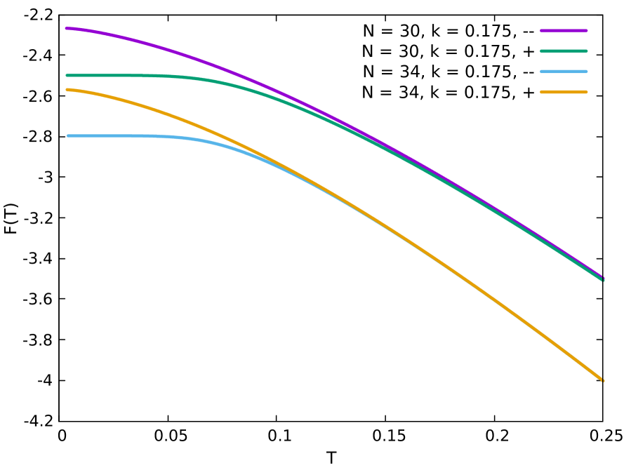
Figure 5: Free energy as a function of temperature for $N=30$ and $34$ Majoranas with positive and negative parity and different values of $k$. The observed temperature independent part of the free energy has its physical origin in the gap between the ground state and the first excited state.

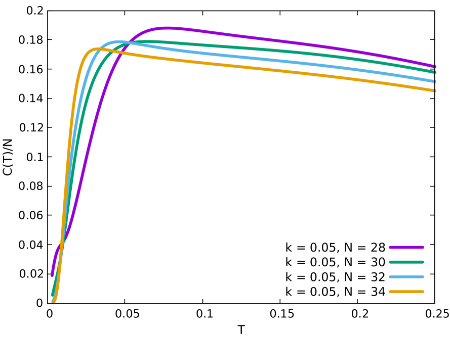
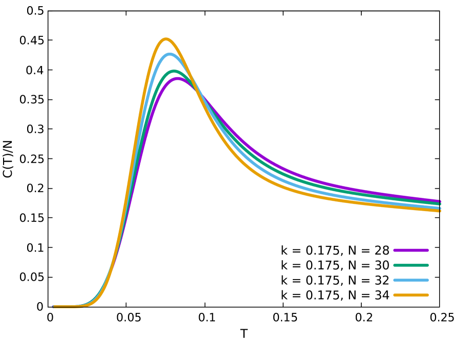
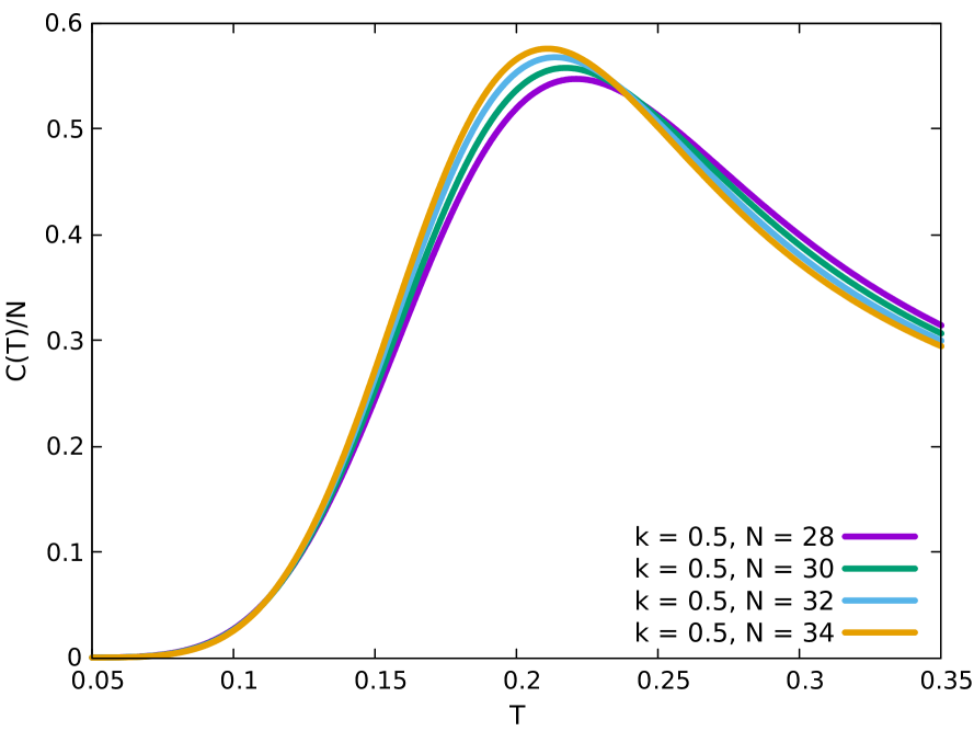
Figure 6: Specific heat as a function of temperature for different values of $N$. For $k_{c}=0.175$ (central) we observe that as $N$ increases, the observed peak becomes increasingly narrow which suggests the existence of the phase transition. For larger $k$ (right) the peak is broad which suggests a crossover. For small $k$ (left), finite size effects seems to be stronger and we cannot reach any firm conclusion.

At higher temperature, the free energy, corresponding to the chiral block that includes the ground state, starts to decrease and becomes increasingly close to the one corresponding to the other chiral block. The temperature at which the two becomes close gives a rough estimation of the critical temperature of the Hawking-Page transition from the graviton gas to the black hole background. A more accurate estimation of the critical temperature can be obtained from the specific heat. For a first order phase transition, the specific heat diverges at the transition, for a second order transition it shows a finite jump and for higher order phase transitions, the specific heat is smooth.

In Fig. 6, we show results for the size dependence of the specific heat for different values of $k$. We note that thermodynamic phase transitions only occur in the $N\to\infty$ limit so information about the size dependence is necessary for a correct understanding of the transition. For large couplings, the specific heat has a broad maximum around the value of the gap, with a weak size dependence. Although the range of sizes is rather limited, this is a strong indication of a crossover, not a transition. For very weak coupling $k=0.05$, the maximum is almost unnoticeable for $N=28$ which suggests that larger couplings or larger sizes are necessary for the wormhole phase to occur. Even for a larger $N=34$, there is only a slight indication of a gap in the spectrum and no clear signature of the transition. Larger values of $N$ are necessary to reach any firm conclusion. For a coupling strength of $k\approx 0.2$ around the one for which we have observed a qualitative change in the ground state, there is a sharp jump of the specific heat for temperatures of the order of the gap. The jump in the specific heat is noticeably sharper as $N$ increases which strongly suggests a phase transition takes place.

Figure 7: Free energy $F$ of the model Eq. (3) versus temperature $T$. The two free energies, computed by solving the Schwinger-Dyson equations by raising and lowering the temperature, with a temperature step of ${dT}=5\cdot 10^{-6}$, intersect at an angle. The full free energy then develops a kink, which signals a first order phase transition around the critical point $k_{c}=0.175$.

IV.2 Solution of Schwinger-Dyson Equations

The above analysis, though illustrative, is not conclusive because of the limited size we can study by exact diagonalization. In order to gain a more quantitative understanding, we have computed the free energy and specific heat in the large $N$ limit by solving the Schwinger-Dyson equations numerically. The details of this calculation have been already explained in great detail in Maldacena and Qi (2018), to which we refer. The purpose of this section is to perform a more precise analysis around the critical coupling $k_{c}$.

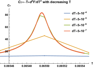
Figure 8: Specific heat of the Hamiltonian Eq. (3) versus temperature. The first order phase transition suddenly turns to a sharp but smooth crossover slightly above the critical value, $k_{c}=0.177$. By taking a very small temperature step to the very small value of $dT=510^{-7}$, the peak in the specific heat turns out to be finite and smooth.

We have found that up to $k=k_{c}\approx 0.175$ the system undergoes a first order phase transition. In order to reach this conclusion we have carried out a careful analysis of the dependence of the derivative of the free energy on the temperature step: the first order phase transition is clearly visible by noticing that, up to $k=k_{c}$, the free energy shows a hysteresis curve as function of the temperature, see Fig. 7.

The critical value of $k_{c}\sim 0.175$ is consistent with the one, obtained in the previous section, at which the ground state changes qualitatively. We have also observed, see Fig. 8, that for slightly larger values of $k\geq 0.177$, this first order phase transition turns out to be a sharp but smooth crossover, which becomes broader with increasing $k$. To reach this conclusion, it has been necessary to study how the peak in the specific heat behaves when decreasing the temperature step: as shown in Fig. 8, by further decreasing the temperature step to the very small value of $dT=5\cdot 10^{-7}$, the peak turns out to be a sharp, but smooth, crossover. We therefore conclude that the window for a hypothetical second order phase transition must be very narrow, $0.175\leq k\leq 0.177$. We note that our results are in perfect agreement with those of Azeyanagi et al. (2018), where a detailed analysis of the Schwinger-Dyson equations associated with a very similar model without disorder was carried out.

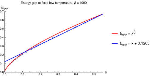
Figure 9: The energy gap, computed at fixed low temperature, as a function of the coupling $k$. We see a crossover from the power law dependence $E_{\text{gap}}\sim k^{2/3}$ to the linear dependence $E_{\text{gap}}\sim k$. This change of behavior was first reported in Ref. Maldacena and Qi (2018).

We have also computed, see Fig. 9, the energy gap $E_{g}$ between the ground state and the first excited state as function $k$ for a fixed low temperature by a careful fitting of the exponential decay of the relevant Green’s function. The same computation has been already performed and explained in Maldacena and Qi (2018). Here, we just reproduce the result for completeness. The dependence of the gap on the coupling $k$ is a further confirmation of the existence of a transition. Around $k\sim k_{c}$ we observe a change of behavior from $E_{g}\propto k^{2/3}$ for $k\ll k_{c}$ to $E_{g}\propto k$ for $k\gg k_{c}$. The latter linear behavior is expected if the gap is due to direct hopping induced by the coupling term in the Hamiltonian which is one-body (two Majoranas) and therefore non-interacting.

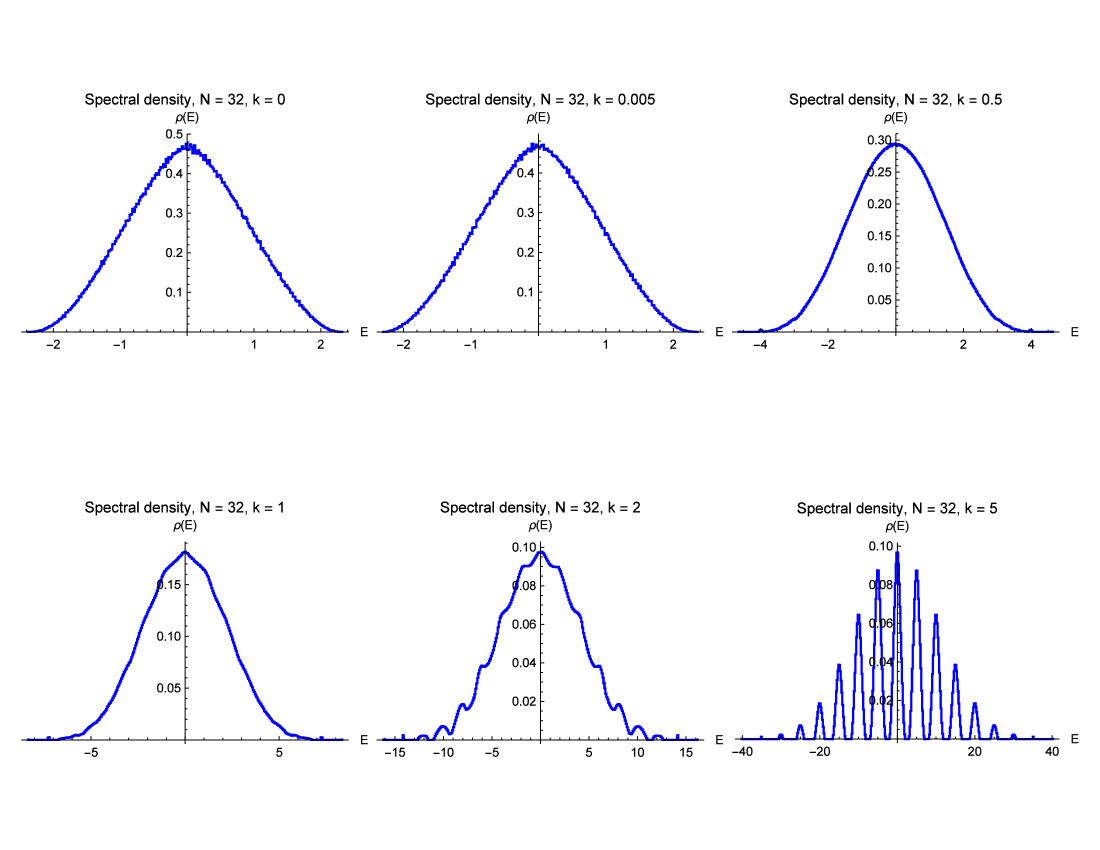
Figure 10: Density of states as a function of the coupling $k$. For sufficiently large $k$ the spectral density splits into separate blobs centered around the eigenvalues of the spin operator. In this region of parameters, no Hawking-Page transition occurs, and the interactions becomes increasingly weak with respect to the hopping between the left and right SYK model.

Physically, by increasing the coupling $k$, we are effectively reducing the many-body interaction inside each SYK model in favor of a direct coupling between the two SYK models which is a diagonalizable one-body (two Majoranas) interaction. This is vaguely reminiscent of a Gross-Witten transition Gross and Witten (1980b), or a BEC-BCS crossover Bourdel et al. (2004), where the reduction of the interaction strength induces a higher order transition or just a crossover.

For larger $k>1$, we have found, see Fig. 10, that the spectral density starts to split into different regions. There is a simple explanation of this phenomenon. The interaction term in the Hamiltonian, which becomes dominant in the large $k$ limit, is proportional to the spin operator which has a discrete spectrum with large degeneracies (see (17)). Therefore we expect that, in this region, the spectral properties are largely controlled by this coupling term and the interactions inside each of the SYK models spread out the degenerate states. Since the eigenvalues of the coupling term range from $-kN/4$ to $kN/4$, we expect the full spectrum of the model to cluster around these few eigenvalues which leads to the appearance of the above mentioned blobs in the spectral density. This is exactly what we observe in the large $k$ limit (see Fig. 10).

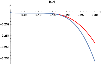
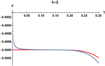
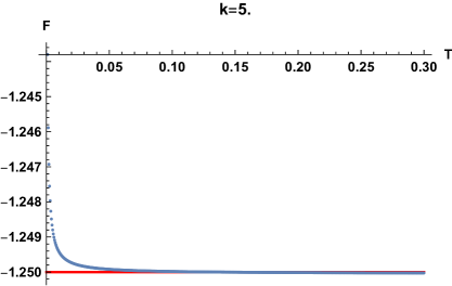
Figure 11: Comparison of the free energy, numerically obtained from the Schwinger-Dyson equation (light blue line), with the analytic expression Eq. (43) for large $k$ (red line). Here, the free energy is normalized such that the plateau value coincides with $-k/4$.

The free energy can be computed analytically in the limit $k\rightarrow\infty$ as follows. If we ignore the SYK terms, we are left with the discrete spectrum just given by Eq. (17), for which the free energy is given by

$$F=-\frac{1}{\beta}\log\sum_{p=0}^{N/2}{\frac{N}{2}\choose p}e^{-\beta k(-N/4+p)}=-\frac{k}{4}-\frac{1}{2\beta}\log(1+e^{-\beta k}).$$ (43)

In Fig. 11, we compare the numerical free energy for $k=1,\;2$ and $5$ with this analytical approximation and find that the agreement becomes excellent around $k\sim 5$.

All these results indicate that the physical reason for the termination of the Hawking-Page transition is just the gradual reduction of the interaction strength. This is a strong indication that a gravity interpretation is restricted to low temperatures and weak coupling where the first order transition takes place.

V Level statistics

We now turn to the study of level statistics, with the main aim to characterize the dynamics in the traversable wormhole phase observed in the low temperature limit of the free energy. For that purpose, we obtain the exact spectrum of the model by exact diagonalization techniques for up to $N=34$ Majoranas. We are especially interested in the spectral correlations of the smallest eigenvalues above the ground state, which are likely to be closely related to gravitational modes of the wormhole phase.

For a meaningful analysis of spectral correlations it is in general necessary to unfold the spectrum so that the mean level spacing is the same across the spectrum. For that purpose, we employ the splines method that fits locally consecutive subsets of many $(>10)$ eigenvalues with low order polynomials. Results are insensitive to the degree of the fitting polynomials.

We aim to study the evolution for long times, of the order of the Heisenberg time, in order to find the range of applicability of random matrix results, a feature of quantum chaotic systems, rather than finite size deviations from it. Hence, we will focus on short range spectral correlators, such as the level spacing distribution, $P(s)$, and the adjacent gap ratio. The former is defined as the probability to find two consecutive eigenvalues $E_{i},E_{i+1}$ at a distance $s=(E_{i+1}-E_{i})/\Delta$ (with $\Delta$ the average local level spacing). For a fully quantum chaotic system it is given by Wigner-Dyson statistics Mehta (2004) which is well approximated by the so called Wigner surmise which depends on the universality class Guhr et al. (1998). For the Gaussian Orthogonal Ensemble (GOE), corresponding to systems with time reversal invariance, it is given by: $P_{\mathrm{W,GOE}}(s)\approx\frac{\pi}{2}s\exp(-\pi s^{2}/4).$ For an insulator, or a generic integrable system, it is given by Poisson statistics, $P_{\mathrm{P}}(s)=e^{-s}$. The adjacent gap ratio is defined as Luitz et al. (2015); Oganesyan and Huse (2007); Bertrand and García-García (2016),

$$r_{i}=\frac{\min(\delta_{i},\delta_{i+1})}{\max(\delta_{i},\delta_{i+1})}$$ (44)

for the ordered spectrum $E_{i-1}<E_{i}<E_{i+1}$ where $\delta_{i}=E_{i}-E_{i-1}$. For a Poisson distribution it is equal to $\left\langle r\right\rangle_{\mathrm{P}}\approx 0.386$ while for a random matrix ensemble it depends on the symmetry class, with $\langle r\rangle\approx 0.530$ for the GOE Atas et al. (2013). The advantage of $\langle r\rangle$ over $P(s)$, is that it does not require to unfold the spectrum. The adjacent gap ratio was also studied in Numasawa (2019) for another model related to the traversable wormhole Kourkoulou and Maldacena (2017).

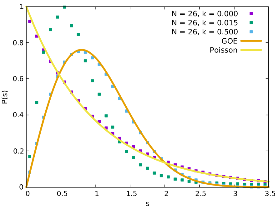
Figure 12: Nearest neighbor spacing distribution $P(s)$ for $N=26$ and different $k$’s in the bulk of the spectrum. As $k$ increases, we observe a crossover from Poisson statistics to the $GOE$ prediction typical of a quantum chaotic system.

We note that for a correct analysis of spectral correlations it is necessary to consider only eigenvalues with the same (good) quantum number. This means that we have to consider eigenvalues only of a given spin and parity sector. Due to the block structure of the Hamiltonian, it is straightforward to select eigenvalues of the same parity. For the spin symmetry, we could not find a numerically inexpensive method to go beyond comparatively small sizes $N=28$. We avoid this problem by introducing an asymmetry in the couplings ($\alpha=1.15$ in Eq. (3)) between left and right SYK models. It has been argued Maldacena and Qi (2018) that the main features of the model, including the existence of a gapped phase, though with a smaller gap, for low temperature which is a signature of the wormhole phase, are robust to a small interaction strength asymmetry which breaks the spin symmetry. We start our analysis of level correlations with the case of very small coupling.

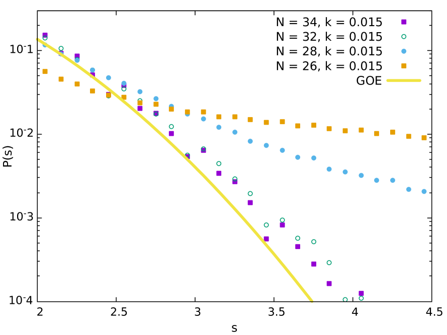
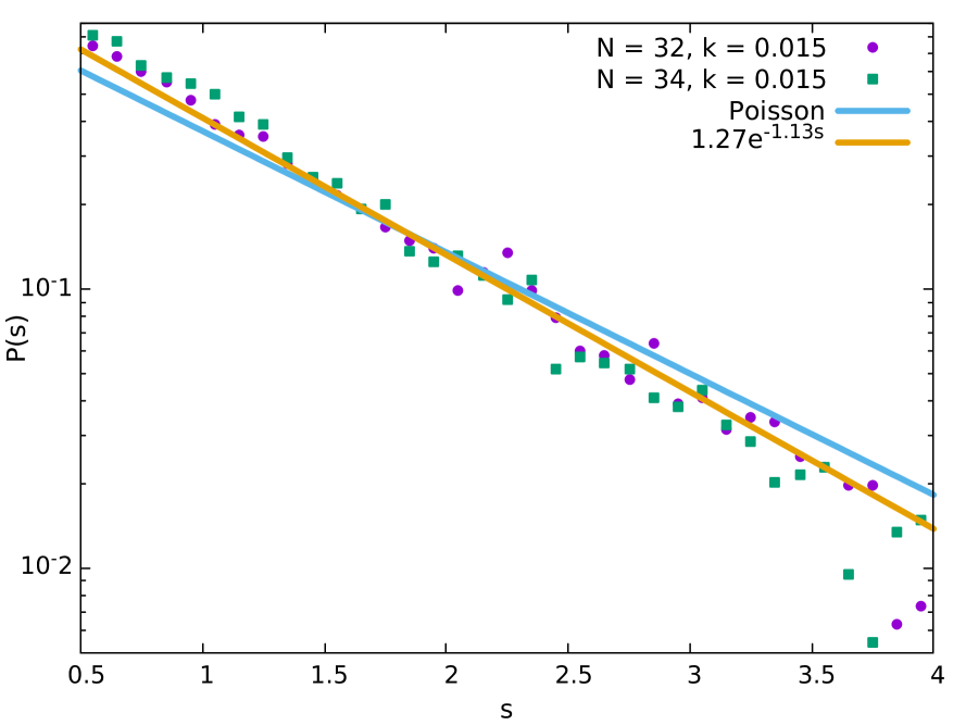
Figure 13: Left: The nearest neighbor spacing distribution, $P(s)$, for small $k$ and different values of $N$ in the bulk of the spectrum. The agreement with the random matrix prediction becomes better as $N$ increases. This is a strong indication that, in the bulk of the spectrum, Poisson statistics for $k=0$ is not robust to a small coupling between the left and right SYK models, namely, the system is always quantum chaotic in the high temperature limit. Right: The nearest spacing distribution, $P(s)$, for small $k$ and $N=32$ or $N=34$ for approximately the lowest $0.1\%$ of the eigenvalues. Agreement with Poisson statistics is very good. This is a strong indication that the infrared limit of the spectrum for sufficiently small $k$ is similar to that for $k=0$ corresponding to two black holes.

V.1 Small $k$

For $k=0$, the eigenvalues of the full Hamiltonian for a given chirality have degeneracies that depend on the value of $N$. For example, we find a two fold or four fold degeneracy $N=20$, and a two fold degeneracy for $N=24$ and $N=32$. Once the degeneracy is removed, we have found, see Fig. 12, spectral correlations in the bulk are well described by Poisson statistics. This is the expected behavior for a system which is defined as the tensor product of two many-body quantum chaotic systems whose spectral correlations are described by random matrix theory. For very small $k\ll 2^{-N/2}$, the spectral degeneracy is barely lifted. As a consequence, the distance between eigenvalues that were degenerate for $k=0$ is much smaller than that between neighboring eigenvalues which makes the analysis of level statistics difficult. For $k\lessapprox 2^{-N/4}$, the degeneracy is already lifted, so the statistical analysis does not require any artificial pruning of the spectrum. In this region, the level statistics in the tail and in the bulk of the spectrum are qualitatively different.

In Fig. 13, we plot the nearest neigbor spacing distribution in the bulk of the spectrum for small $k$ and different values of $N$. Level repulsion is observed in all cases, but for $N=26$ and $N=28$ the decay for large distances is clearly exponential with an exponent close to the one corresponding to a Poisson distribution. However for $N=32$ and $N=34$ we find good agreement with random matrix correlations. Although a careful finite size scaling analysis would be necessary to reach a final conclusion, the latter is a strong suggestion that in the bulk of the spectrum, corresponding to high temperatures, even a small coupling $k$, makes the system quantum chaotic. However, see Fig. 13, it seems that the lowest eigenvalues in the same region of small $k$, for $N=32$ and $N=34$ are correlated to Poisson statistics like for $k=0$. Rather than a metal-insulator transition at a certain value of $k$, this behavior suggests that for sufficiently weak coupling the two SYK’s, each of them quantum chaotic, are effectively disconnected systems for low energies (tail) while for sufficiently high energies (bulk) the behavior is similar to a single quantum chaotic system whose levels are correlated according to random matrix theory. It is tempting to speculate that this indicates a transition from two black holes to one black hole for sufficiently high temperatures. However, the fact that we do not have a clear geometrical understanding on how this transition can occur, together with the limited range of $N$ values which we could study numerically, prevents us to reach any firm conclusion.

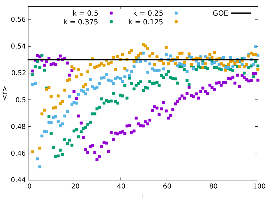
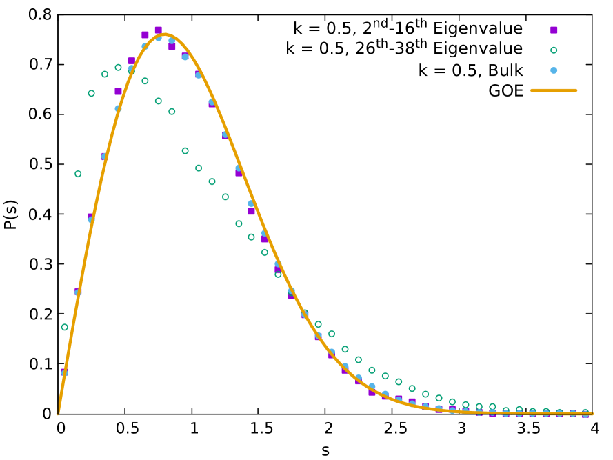
Figure 14: Left: Adjacent gap ratio $\langle r\rangle$, Eq. (44), for $N=26$ and different values of $k$ for the infrared part of the spectrum. We observe that, as $k$ increases, some of the lowest eigenvalues become correlated according to the random matrix theory. Except for $k\approx 0$, the bulk of the spectrum is correlated according to the random matrix prediction. Right: Results for the level spacing distribution $P(s)$ fully confirm the agreement with the Wigner surmise typical of random matrix spectral correlations.

Summarizing, our results show that, while in the bulk of the spectrum a very small value of $k$ is sufficient to induce the transition from Poisson statistics to random matrix theory spectral correlations, in the tail of the spectrum, Poisson statistics is robust, and a larger coupling is necessary to induce the transition to level statistics described by random matrix theory. We investigate this case next.

V.2 Critical $k$

As $k$ increases, the bulk of the spectrum is still correlated according to random matrix theory with no quantitative change from the region of small $k$ investigated previously. For this reason, we will focus exclusively on the spectral correlations in the tail of the spectrum.

In Fig. 14 we depict results for the average adjacent gap ratio $\langle r\rangle$ with different values of $k$ for the chiral block that includes the ground state. In the tail of the spectrum we do observe clear deviations from the GOE prediction that become gradually smaller as $k$ increases. Interestingly, for $k\approx 0.14$, the ratio for the lowest eigenvalues becomes suddenly very close to the GOE value while the subsequent eigenvalues still deviate substantially from it. A further increase of the coupling $k$ leads to more of the lowest eigenvalues becoming correlated according to the GOE while the subsequent ones still show deviations. Finally, for $k\sim 1$, all eigenvalues in the spectrum are GOE correlated. We stress that the value of $k$ for which the lowest eigenvalue becomes GOE correlated is very similar to the one at which the termination of the Hawking-Page transition, between the traversable wormhole and the black hole phase, takes place. This is a strong suggestion that deviations from random matrix theory in the tail, with values close to Poisson statistics, may be related to the wormhole phase and that the sudden appearance of the GOE correlated eigenvalues deep in the infrared may signal an instability of the wormhole phase. This instability might be expected close to the transition to a black hole phase.

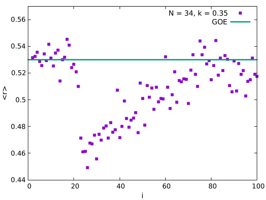
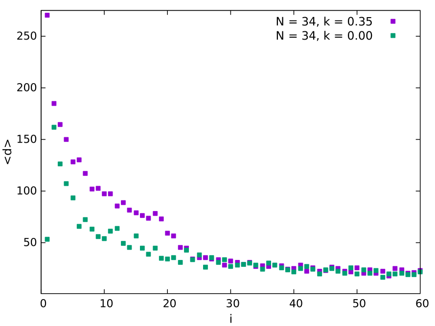
Figure 15: Left: Adjacent gap ratio $\langle r\rangle$, Eq. (44), for $N=34$ and $k=0.35$. More low-lying eigenvalues are correlated according to random matrix theory for increasing $N$. Right: Local average spacing $\langle d_{i}\rangle=\langle E_{i+1}-E_{i}\rangle$ for $N=34$, $k=0.35$ rescaled by the total average mean level spacing. Roughly speaking, only the local spacing involving the lowest $25$ eigenvalues is $k$ dependent. This is also the number of eigenvalues which are correlated according to random matrix figure in the left figure.

As a further check that random matrix theory describes the level statistics of the lowest eigenvalues for $k>0.14$, we compare the level spacing distribution $P(s)$ of these eigenvalues with the Wigner surmise. Results, depicted in Fig. 14 confirm that for $k\sim 0.5$, the level spacing distribution for the lowest eigenvalues is in excellent agreement with the Wigner surmise $P_{\mathrm{W,GOE}}(s)$.

The coupling between the left and right site is a relevant perturbation which we expect to become dominant in the tail of the spectrum. Interestingly, in Ref. Maldacena and Qi (2018) it was reported that, assuming $N$ fixed and $k$ sufficiently large, some of the lowest energy excitations of the effective Hamiltonian are of gravitational origin and not related to the breaking of conformal symmetry. Physically this corresponds to excited states of the wormhole geometry. It is tempting to speculate that there is a connection between these excitations of the wormhole geometry and the deviations from random matrix theory in the tail of the spectrum below the critical coupling. If this picture applies, these gravitational modes related to the wormhole phase are not quantum chaotic and the sudden transition to random matrix theory in level statistics is a dynamical aspect of the thermodynamic Hawking-Page transition. That would imply that random matrix theory, and therefore quantum ergodicity, is only a signature of quantum black holes but not of an AdS graviton gas. In other words, the Hawking-Page transition can be dynamically characterized as a chaotic-integrable transition.

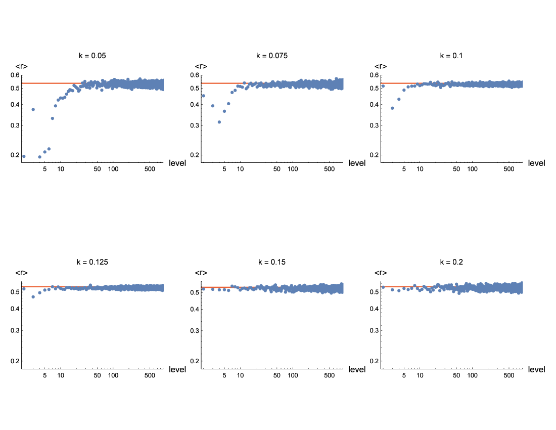
Figure 16: Adjacent gap ratio $\langle r\rangle$, Eq. (44) for $N=28$, ${\alpha}=1$ in Eq.( 3) and different values of the coupling parameter $k$. We employ only eigenvalues corresponding to the sector of lowest spin $S=-N/4$ that includes the ground state. Results are qualitatively similar to those of different couplings. Deviations from GOE random matrix results (orange line) are observed for small $k$ which gradually disappear as $k$ approaches the critical point $k_{c}\sim 0.17$ where the Hawking-Page transition terminates.

In order to test this hypothesis, we compare explicitly the number of eigenvalues with random matrix like correlations with the spectral density (one point function) in that region. For that purpose, we employ again the adjacent gap ratio $\langle r\rangle$, but with a larger $N=34$, so that more eigenvalues show the anticipated anomalous behavior. Regarding the spectral density, for which the prediction of gravitational excitations of Ref. Maldacena and Qi (2018) applies, we employ the local spectral density and $\langle d\rangle\equiv\langle E_{i+1}-E_{i}\rangle$. Results, depicted in Fig. 15, clearly show that the number of eigenvalues with random matrix correlations is in good agreement with the number of eigenvalues whose $\langle d\rangle$ shows a pronounced dependence on $k$ for sufficiently large $k$. Although further research is required to confirm this point, this quantitative agreement is encouraging. It strongly suggests that full quantum ergodicity is typical only of black holes, while other geometries like quantum wormholes may be closer to Poisson statistics typical of integrable dynamics. We now move to study level statistics for $\alpha=1$ in order to confirm that these findings are not particular to the value of $\alpha\sim 1$ used in previous sections.

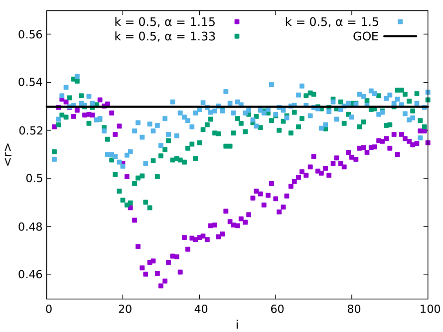
Figure 17: Adjacent gap ratio $\langle r\rangle$, Eq. (44), for $N=26$ and different values of the asymmetry parameter. We observe that as the asymmetry increases the separation between the low lying eigenvalues gradually disappears.

V.3 Dependence of Level correlations on $\alpha=1$

To study level correlations in this case, the additional global spin symmetry for equal couplings makes it necessary to only consider eigenvalues with the same spin mod $4$ eigenvalue, in this case the block containing $S=-N/4$ which includes the ground state. This requires an explicit calculation of eigenvectors which further limits the maximum $N$ which we can reach numerically to $N=28$ also taking into account that we need at least $500$ disorder realizations to have relatively good statistics. Results for $\langle r\rangle$, shown in Fig. 16, clearly show similar features as in the slightly asymmetric case: deviation from GOE for small $k$ followed by the sudden appearance of the lowest eigenvalues correlated according to random matrix theory at around the same value $k_{c}\sim 0.15$. However, for $N=28$, the crossover region is very narrow, only the two lowest eigenvalues become GOE correlated before the full spectrum becomes GOE correlated, and the distinction between the tail and the bulk of the spectrum becomes more difficult to identify.

The spin symmetry is broken by the coupling asymmetry. However, as mentioned previously, a small asymmetry does not change the physics of the model but makes it technically easier to study the level statistics. In order to confirm this point more explicitly, we investigate the dependence of level statistics on the asymmetry parameter $\alpha$ in Eq. (3). In Fig. 17, we depict results for the adjacent gap ratio and different values of ${\alpha}$. As $\alpha$ increases, the differences between the tail and bulk of the spectrum becomes increasingly small. Eventually, the full spectrum becomes correlated according to random matrix theory even with a comparatively weak coupling. Physically this is an indication that the wormhole phase related to the graviton gas disappears if the asymmetry between left and right is sufficiently strong. This is consistent with the results of Ref. Maldacena and Qi (2018) where it was found that both the ground state energy gap and the left-right correlation decreases as the asymmetry increases. However further research is required to determine whether there is a sharp maximum value of the asymmetry for the wormhole phase to occur.

VI Outlook and Conclusions

We have studied a coupled two-site SYK model whose gravity dual is conjectured to be Maldacena and Qi (2018) a traversable wormhole geometry in the low temperature, small coupling, limit and dual to a black hole geometry for sufficiently strong coupling or high temperature. We have analyzed the spectral and thermodynamic properties of this model and have found that it has a previously unknown discrete spin symmetry which among other things is important for the analysis of level correlations.

In Ref. Maldacena and Qi (2018), it was shown that the phase transition of this model is first order for weak coupling and seems to terminate for stronger coupling. An important point in the analysis of Maldacena and Qi (2018) is that the ground state in the wormhole phase is well approximated by a TFD state. In this paper we have found that except in the limit of strong coupling between the two SYK models, TFD is never a good approximation of the ground state for the number of Majoranas ($N\leq 34$) that we can investigate by exact diagonalization. For weaker coupling, coefficients of the expansion of the ground state in a tensor product of the two separate SYK models have a slower power law decay, in contrast to the fast exponential decay with the energy expected in a TFD state. Physically, this suggests a non-thermal state with entanglement properties qualitatively different from those of the TFD state. As the coupling $k$ increases, the overlap of the ground state with the TFD state decreases with a minimum at $k_{c}\sim 0.1$. For stronger coupling, the ground state becomes increasingly well approximated by the TFD state. In this large coupling limit, eigenstates of the associated spin operator with the lowest eigenvalues are both close to the ground state of the system and to a TFD state at infinite temperature. Note that the deviations from the TFD state at weak coupling mentioned above do not implicate that the overlap between the ground state and the TFD state is small. The reason is that for small coupling the strength of the wave function in a tensor basis of $H_{SYK}\otimes H_{SYK}$ is concentrated in only one or a few components of the eigenvectors which determine the overlap with the TFD state independently of the distribution in energy of the components.

We have also studied thermodynamic properties and level statistics that provide valuable information on the long time dynamics of the model. Regarding thermodynamic properties, we have fully confirmed Maldacena and Qi (2018) that the transition is of first order for weak coupling and it terminates abruptly at $k_{c}\sim 0.2$. A careful analysis of the free energy and specific heat shows that for stronger coupling, at fixed temperature, there is no second order transition but just a sharp crossover. To a good approximation, this is also the value of the coupling where the $k$ dependence of the energy gap changes from a power law to a linear dependence which is typical of a non-interacting system. In the strong coupling limit, the spectral density develops well separated blobs centered around the eigenvalues of the spin operator.

Level statistics are also affected by the coupling strength. For $k<k_{c}$, we observe in the tail of the spectrum important deviations from the random matrix prediction, that we speculate, is an indication that gravitational bound states related to the wormhole geometry are not quantum chaotic. Around the transition we have observed that, suddenly, the lowest eigenvalues become correlated according to random matrix theory. This quantum chaotic behavior is an expected feature García-García and Verbaarschot (2016) of quantum black hole backgrounds. For larger $k$, the number of eigenvalues in the tail of the spectrum, that is well described by random matrix theory, increases. Eventually, for $k\sim 1$, the full spectrum is correlated according to the random matrix theory prediction. Physically, random matrix spectral correlations are an indication of quantum chaotic features and full quantum ergodicity which is believed to be a distinctive feature of quantum black holes. Therefore, the sudden appearance of random matrix correlations deep in the infrared may be an indication of the instability of the wormhole phase towards the black hole phase. On the (quantum) gravity side, the exact meaning of a sharp crossover between the two geometries is unclear.

In the opposite limit of very small $k$, well below the transition $k=k_{c}$, we observe Poisson statistics for very small coupling strength $k_{c}\lessapprox 0.03$ (once the degeneracies are removed) which suggests that, at least in the range of finite $N$ we can explore, a minimum coupling is necessary to access the wormhole phase. For larger coupling, the bulk of the spectrum becomes quickly correlated according to random matrix theory while deviations in the tail, very likely related to the wormhole phase, are still present until the transition occurs. We did not manage to quantitatively understand these deviations. The limited range of sizes we can explore numerically prevent us to perform a finite size scaling analysis. Additional research is required to clarify whether this limit of very small $k$ or the region of sudden appearance of random matrix correlations mentioned above broadens the phase diagram of the system.

We note that the coupling term is one-body and therefore integrable. This leads us to speculate that for a fixed temperature, the effective interactions among left and right Majoranas decrease as the coupling $k$ increases. It is tempting to speculate that the full phenomenology of the model is consistent with a strong-weak coupling transition as $k$ increases such as the Gross-Witten transition Gross and Witten (1980b) or the BEC-BCS crossover Bourdel et al. (2004) observed in cold atom physics.

Interesting problems for further research include, the universality of these results for non-minimal couplings between the two sites or to clarify whether similar physics is observed in supersymmetric analogues of this problem. Another still unresolved problem is the gravity dual interpretation, if any, of the sharp crossover that we observed around the transition. More specifically, it would be interesting to clarify whether both geometries can somehow coexist in this region or simply the system ceases to have a gravity dual interpretation. Another point which would be nice to investigate further is the study of the level statistics for the case of equal couplings: in particular, it would be important to push the numerical studies to larger $N$ to see if the distinction between the bulk and the tail of the spectrum becomes more prominent. To reach this goal, we believe that the method of Gur-Ari et al. (2018) could be useful. The non TFD nature of the ground state for weak coupling, characterized by a power law decay of the coefficients in a tensor product basis, such as entanglement properties, deserves further investigation as well. Does this power law dependence have a gravity dual interpretation? We plan to address some of these problems in the near future.

Appendix A Notations for Gamma matrices

The Gamma matrices in (4) are defined as usual

$$\{\Gamma_{i},\Gamma_{j}\}=2\delta_{ij}$$ (45)

For each SYK we have a chiral operator

$$\Gamma_{5}^{R}=i^{-N/4}\prod_{k=1}^{N/2}\Gamma_{k},\qquad\Gamma_{5}^{L}=i^{-N/4}\prod_{k=1}^{N/2}\Gamma_{k+N/2},$$ (46)

the charge conjugation symmetry operators are defined as

$$C^{R}=\prod_{k=1}^{N/4}\Gamma_{2k}K,\qquad C^{L}=\prod_{k=1}^{N/4}\Gamma_{2k+N/2}K,$$ (47)

with $K$ the complex conjugation operator. They satisfy the commutation relations

$$[H_{R},\Gamma_{5}^{R}] = 0,\qquad[H_{L},\Gamma_{5}^{L}]=0,$$ (48)

$${[H_{R},\Gamma_{5}^{L}]} = 0,\qquad[H_{L},\Gamma_{5}^{R}]=0,$$ (49)

$$\{S,\Gamma_{5}^{L}\} = 0,\qquad\{S,\Gamma_{5}^{R}\}=0,$$ (50)

$${[H_{R},C^{R}]} = 0,\qquad[H_{L},C^{L}]=0,$$ (51)

We also define

$$\Gamma_{5}=\Gamma_{5}^{R}\Gamma_{5}^{L},$$ (52)

which is a symmetry of the total Hamiltonian. The chiral projectors are given by

$$P^{R}=\frac{1}{2}(1+\Gamma_{5}^{R}),\qquad P^{L}=\frac{1}{2}(1+\Gamma_{5}^{L}),\qquad$$ (53)

If $N/4$ is even, the charge conjugation operator commutes with the corresponding projection operator, but this is not the case when $N/4$ is odd. Then $\{\Gamma_{5}^{R},C^{R}\}=0$ and if we have an eigenstate of $H_{R}$,

$$H_{R}|n\rangle=\lambda|n\rangle,\quad{\rm with}\quad\Gamma_{5}|n\rangle=g_{5}|n\rangle$$ (54)

then also

$$H_{R}C_{R}|n\rangle=\lambda C_{R}|n\rangle,$$ (55)

but now

$$\Gamma_{5}^{R}C^{R}|n\rangle=-g_{5}C^{R}|n\rangle.$$ (56)

Appendix B Alternative derivation of $S$ mod 4 symmetry

The coupled model has an additional spin symmetry

$$[e^{i\frac{\pi}{2}S},H_{R}+H_{L}+kS]=0,$$ (57)

with

$$e^{\frac{\pi i}{2}S}=\prod_{k=1}^{N/2}\frac{1}{\sqrt{2}}(1+\Gamma_{k+N/2}\Gamma_{k}).$$ (58)

To see that a product of the four factors

$$1+\Gamma_{k+N/2}\Gamma_{k}$$ (59)

also commutes with terms from the Hamiltonian that contain the index $k$, i.e. terms of the from

$$\Gamma_{k+N/2}\Gamma_{l+N/2}\Gamma_{m+N/2}\Gamma_{n+N2}+\Gamma_{k}\Gamma_{l}\Gamma_{m}\Gamma_{n}$$ (60)

it is simplest to use the decomposition

$$\Gamma_{k+N/2}\Gamma_{l+N/2}\Gamma_{m+N/2}\Gamma_{n+N/2}+\Gamma_{k}\Gamma_{l}\Gamma_{m}\Gamma_{n}=\frac{1}{2}(P_{kl}P_{mn}+Q_{kl}Q_{mn})$$ (61)

with

$$P_{kl} = \Gamma_{k}\Gamma_{l}+\Gamma_{k+N/2}\Gamma_{l+N/2},$$ (62)

$$Q_{kl} = \Gamma_{k}\Gamma_{l}-\Gamma_{k+N/2}\Gamma_{l+N/2}.$$ (63)

It is clear that each of the factors in (59) commutes with the $P_{kl}$. They do not commute separately or even pairwise with the $Q_{kl}$ term. The commutator can be rewritten as

$$[F_{kl}F_{mn},Q_{kl}Q_{mn}]=[Q_{kl},F_{kl}]F_{mn}Q_{mn}+Q_{kl}F_{kl}[Q_{mn},F_{mn}]$$ (64)

with $F_{kl}=-(1+\Gamma_{k+N/2}\Gamma_{k})(1+\Gamma_{l+N/2}\Gamma_{l})/2$. We have that

$$[Q_{kl},F_{kl}] = 2(\Gamma_{k}\Gamma_{l+\frac{N}{2}}-\Gamma_{l}\Gamma_{k+\frac{N}{2}}),$$

$$F_{kl}Q_{kl} = \Gamma_{l}\Gamma_{k+\frac{N}{2}}-\Gamma_{k}\Gamma_{l+\frac{N}{2}},$$

$$Q_{kl}F_{kl} = \Gamma_{k}\Gamma_{l+\frac{N}{2}}-\Gamma_{l}\Gamma_{k+\frac{N}{2}},$$

so that the commutator vanishes. This proves the $S$ mod 4 symmetry.

Appendix C Ground state of the spin operator for $N/2\mod 8=2$

In this appendix we derive that the ground state of the spin operator $N/2\mod 8=2$ is given by

$$|S=-N/4\rangle=\frac{1}{\sqrt{L(N/2)}}\sum_{n,\pm}|n_{\pm}\rangle_{L}\otimes|n_{\mp}\rangle_{R}$$ (66)

for an appropriate choice of the phases of the states $|n_{\pm}\rangle_{L,R}$.

Let us consider the case $N=20,28,\cdots$ ($N/2\mod 8=2$). In this case the charge conjugation matrix anti-commutes with the chiral $\gamma$ matrix

$$\{\gamma_{c},C\}$$ (67)

with $\gamma_{c}=i^{-\frac{N}{4}}\gamma_{1}\gamma_{2}\cdots\gamma_{{N}/{2}}$. Both $\gamma_{c}$ and $CK$ commute with the Hamiltonion of a single SYK system ($K$ is the complex conjugation operator)

$$[H_{\rm SYK},\gamma_{c}]=0,\qquad[H_{\rm SYK},CK]=0$$ (68)

In a chiral basis with eigenvectors ${\widetilde{v}}_{n,\pm}$ of $H_{\rm SYK}$ we thus have that $CK{\widetilde{v}}_{n,\pm}$ is also an eigenvector of $H_{\rm SYK}$ but with opposite chirality because of the anti-commutation relations (67).

We now define the left/right states above as

$$|n_{+}\rangle_{L}={\widetilde{v}}_{n,+},\quad|n_{-}\rangle_{L}=C({\widetilde{v}}_{n,+})^{*},\quad|n_{+}\rangle_{R}=e^{-\frac{\pi i}{4}}{\widetilde{v}}_{n,+},\quad|n_{-}\rangle_{R}=e^{\frac{\pi i}{4}}C({\widetilde{v}}_{n,+})^{*}.$$ (69)

With this convention we obtain

$$\langle m_{\pm}|_{R}\gamma_{i}|n_{\mp}\rangle_{R}=\pm i\langle m_{\pm}|_{L}\gamma_{i}|n_{\mp}\rangle_{L},\quad\langle n_{\mp}|_{L}\gamma_{i}|m_{\pm}\rangle_{L}=(\langle n_{\pm}|_{L}\gamma_{i}|m_{\mp}\rangle_{L})^{*},$$ (70)

where the first equation holds due to the prefactor $\exp{\mp\frac{\pi i}{4}}$ in $|n_{\pm}\rangle_{R}$, and the second equation is a consequence of the relation ${\widetilde{v}}_{n,-}=C({\widetilde{v}}_{n,+})^{*}$. Combining these two equations we find

$$\langle m_{\pm}|_{R}\gamma_{i}|n_{\mp}\rangle_{R}=\pm i\langle n_{\pm}|_{L}\gamma_{i}|m_{\mp}\rangle_{L}.$$ (71)

To show that the state (77) is the ground state of the spin operator we calculate the expectation value

$$\langle S=-N/4|S|S=-N/4\rangle = \frac{i}{2^{N/4+1}}\sum_{i=1}^{N/2}\sum_{m,n,\pm,\pm^{\prime}}\langle m_{\pm}|_{L}\otimes\langle m_{\mp}|_{R}\Gamma_{i}\Gamma_{{N}/{2}+i}|n_{\pm^{\prime}}\rangle_{L}\otimes|n_{\mp^{\prime}}\rangle_{R}$$ (72)

$$= \frac{i}{2^{N/4+1}}\sum_{i=1}^{N/2}\sum_{m,n,\pm,\pm^{\prime}}\langle m_{\pm}|_{L}\gamma_{i}\gamma_{c}|n_{\pm^{\prime}}\rangle_{L}\langle m_{\mp}|_{R}\gamma_{i}|n_{\mp^{\prime}}\rangle_{R}.$$

Since $\gamma_{i}$ flips the chirality, only terms with $\pm^{\prime}=\mp$ contributes:

$$\langle S=-N/4|S|S=-N/4\rangle = \frac{i}{2^{N/4+1}}\sum_{i=1}^{N/2}\sum_{m,n,\pm}(\langle m_{\pm}|_{L}\gamma_{i}\gamma_{c}|n_{\mp}\rangle_{L})(\langle m_{\mp}|_{R}\gamma_{i}|n_{\pm}\rangle_{R})$$ (73)

$$= -\frac{1}{2^{N/4+1}}\sum_{i=1}^{N/2}\sum_{m,n,\pm}(\langle m_{\pm}|_{L}\gamma_{i}|n_{\mp}\rangle_{L})(\langle n_{\mp}|_{L}\gamma_{i}|m_{\pm}\rangle_{L}),$$

where we have used $\gamma_{c}|n_{\pm}\rangle=\pm|n_{\pm}\rangle$ and (71). Now again noticing the fact that $\gamma_{i}$ flips chirality, we can safely replace $\sum_{n}|n_{\mp}\rangle_{L}\langle n_{\mp}|_{L}\rightarrow\sum_{n}(|n_{+}\rangle_{L}\langle n_{+}|_{L}+|n_{-}\rangle_{L}\langle n_{+}|_{L})=1$ in the last line

$$\langle S=-N/4|S|S=-N/4\rangle = -\frac{1}{2^{N/4+1}}\sum_{i=1}^{N/2}\sum_{m,\pm}\langle m_{\pm}|_{L}\gamma_{i}\gamma_{i}|m_{\pm}\rangle_{L}$$ (74)

$$= -\frac{N}{4},$$

which is the lowest eigenvalue of the spin operator.

From Eq. (69) we can derive

$$|n_{-}\rangle_{R} = e^{\frac{\pi i}{4}\gamma_{c}}CK|n_{+}\rangle_{L},$$ (75)

$$|n_{+}\rangle_{R} = e^{\frac{\pi i}{4}\gamma_{c}}CK|n_{-}\rangle_{L},$$ (76)

which allows us to rewrite the TFD state as

$$|S=-N/4\rangle=\frac{1}{\sqrt{L(N/2)}}\sum_{n,\pm}|n_{\pm}\rangle_{L}\otimes e^{\frac{\pi i}{4}\gamma_{c}}CK|n_{\mp}\rangle_{L}.$$ (77)

This is exactly the structure that was used in the general proof (28).

Appendix D Lowest spin state and $|\text{TFD}\rangle_{\beta=0}$ for $N/2\mod 8=4$

We now construct explicitly the lowest eigenstate of the spin operator for $N/2\mod 8=4$. In this case, the spectrum of $H_{SYK}$ with $N/2$ fermions is two-fold degenerate in both blocks, while there are no degeneracies between the upper block and the lower block.

In this case, $H_{\rm SYK}$, the charge conjugation operator $CK$ and the chiral matrix $\gamma_{c}$ are a set of commuting operators that can be diagonalized simultaneously. However, we have that

$$(CK)^{2}=-1,$$ (78)

so that a state $\phi$ and a state $C\phi$ are linearly independent, which explains the two-fold degeneracy of the states (which is the Kramers degeneracy). Let us introduce an extra index $a=1,2$ for this degeneracy and denote the eigenvectors of $H_{\rm SYK}$ as ${\widetilde{v}}_{n,\pm,a}$. They satisfy the orthogonality relations

$$({\widetilde{v}}_{m,\pm,a})^{\dagger}{\widetilde{v}}_{n,\pm^{\prime},b}=\delta_{mn}\delta_{\pm,\pm^{\prime}}\delta_{ab}.$$ (79)

To define the TFD state we choose the left/right states $|n_{\pm,a}\rangle_{L}$, $|n_{\pm,a}\rangle_{R}$ as

$$|n_{\pm,1}\rangle_{L} = {\widetilde{v}}_{n,\pm,1},$$ (80)

$$|n_{\pm,2}\rangle_{L} = C({\widetilde{v}}_{n,\pm,1})^{*},$$ (81)

$$|n_{\pm,1}\rangle_{R} = e^{\pm\frac{\pi i}{4}}|n_{\pm,1}\rangle_{L}=-e^{\frac{\pi i}{4}\gamma_{c}}CK|n_{\pm,2}\rangle_{L},$$ (82)

$$|n_{\pm,2}\rangle_{R} = -e^{\pm\frac{\pi i}{4}}|n_{\pm,2}\rangle_{L}=-e^{\frac{\pi i}{4}\gamma_{c}}CK|n_{\pm,1}\rangle_{L}.$$ (83)

Then we can show

$$\phi=\frac{1}{\sqrt{L(N/2)}}\sum_{n,\pm}(|n_{\pm,1}\rangle_{L}\otimes|n_{\pm,2}\rangle_{R}+|n_{\pm,2}\rangle_{L}\otimes|n_{\pm,1}\rangle_{R})$$ (84)

is the ground state of the spin operator. This follows by using the Eqs. (82) and (83) to rewrite $\phi$ as

$$\phi=-\frac{1}{\sqrt{L(N/2)}}\sum_{n,\pm,a}(|n_{\pm,a}\rangle_{L}\otimes e^{\frac{\pi i}{4}\gamma_{c}}CK|n_{\pm,a}\rangle_{L}.$$ (85)

This is exactly the structure of the state (28), so that the proof applies that it is the ground state of the spin operator.

Appendix E Ground state of spin operator for $N/2\mod 8=0$

In this case $(KC)^{2}=1$ and it is always possible to choose a basis for which

$$CK|n\rangle_{R.L}=|n\rangle_{R,L}.$$ (86)

The phases of the right states will be chosen as

$$|n_{\pm}\rangle_{R}=e^{\frac{\pi i}{4}\gamma_{c}}|n_{\pm}\rangle_{L}.$$ (87)

Then the TFD state is given by

$$|\phi\rangle=\sum_{n,\pm}|n_{\pm}\rangle_{L}e^{\frac{\pi i}{4}\gamma_{c}}|n_{\pm}\rangle_{L}.$$ (88)

The expectation values of the spin operator is given by

$$\langle\phi|S|\phi\rangle = \frac{i}{2}2^{-N/4}\sum_{k=1}^{N/2}\sum_{mn\pm\pm^{\prime}}\langle n_{\pm}|_{L}\gamma_{k}\gamma_{c}|m_{\pm^{\prime}}\rangle_{L}\langle n_{\pm}|_{R}\gamma_{k}|m_{\pm^{\prime}}\rangle_{R}$$ (89)

$$= \frac{i}{2}2^{-N/4}\sum_{k=1}^{N/2}\sum_{mn\pm}\langle n_{\pm}|_{L}\gamma_{k}\gamma_{c}|m_{\mp}\rangle_{L}\langle n_{\pm}|_{L}e^{-\frac{\pi i}{4}\gamma_{c}}\gamma_{k}e^{\frac{\pi i}{4}\gamma_{c}}|m_{\mp}\rangle_{L}$$

$$= \frac{i}{2}2^{-N/4}\sum_{k=1}^{N/2}\sum_{mn\pm}e^{\mp\frac{\pi i}{2}}(\mp)\langle n_{\pm}|_{L}\gamma_{k}|m_{\mp}\rangle_{L}\langle n_{\pm}|_{L}\gamma_{k}|m_{\mp}\rangle_{L}$$

$$= -\frac{1}{2}2^{-N/4}\sum_{k=1}^{N/2}\sum_{mn\pm}\langle n_{\pm}|_{L}\gamma_{k}|m_{\mp}\rangle_{L}\langle m_{\mp}|_{L}\gamma_{k}|n_{\pm}\rangle_{L}$$

$$= -\frac{N}{4}.$$

For the last equality we have used that that the $\gamma$-matrices for $N/2\mod 8=0$ can be chosen real symmetric.

References

- Wigner (1951) E. Wigner, Math. Proc. Cam. Phil. Soc. 49, 790 (1951).
- Bertrand and García-García (2016) C. L. Bertrand and A. M. García-García, Phys. Rev. B 94, 144201 (2016).
- Efetov (1983) K. Efetov, Advances in Physics 32, 53 (1983).
- Bohigas et al. (1984) O. Bohigas, M. J. Giannoni, and C. Schmit, Phys. Rev. Lett. 52, 1 (1984).
- Verbaarschot and Zahed (1993) J. J. M. Verbaarschot and I. Zahed, Phys. Rev. Lett. 70, 3852 (1993).
- Shuryak and Verbaarschot (1993) E. Shuryak and J. Verbaarschot, Nuclear Physics A 560, 306 (1993).
- Maldacena et al. (2016a) J. Maldacena, S. H. Shenker, and D. Stanford, Journal of High Energy Physics 08, 106 (2016a).
- Larkin and Ovchinnikov (1969) A. Larkin and Y. N. Ovchinnikov, Sov Phys JETP 28, 1200 (1969).
- (9) A. Kitaev, “A simple model of quantum holography,” KITP strings seminar and Entanglement 2015 program, 12 February, 7 April and 27 May 2015, http://online.kitp.ucsb.edu/online/entangled15/.
- Maldacena and Stanford (2016) J. Maldacena and D. Stanford, Phys. Rev. D 94, 106002 (2016).
- Bohigas and Flores (1971a) O. Bohigas and J. Flores, Physics Letters B 34, 261 (1971a).
- Bohigas and Flores (1971b) O. Bohigas and J. Flores, Physics Letters B 35, 383 (1971b).
- French and Wong (1970) J. French and S. Wong, Physics Letters B 33, 449 (1970).
- French and Wong (1971) J. French and S. Wong, Physics Letters B 35, 5 (1971).
- Mon and French (1975) K. Mon and J. French, Annals of Physics 95, 90 (1975).
- Benet and Weidenmüller (2003) L. Benet and H. A. Weidenmüller, Journal of Physics A: Mathematical and General 36, 3569 (2003).
- Kota (2014) V. K. B. Kota, Embedded random matrix ensembles in quantum physics, Vol. 884 (Springer, 2014).
- Sachdev and Ye (1993) S. Sachdev and J. Ye, Phys. Rev. Lett. 70, 3339 (1993).
- Sachdev (2010) S. Sachdev, Phys. Rev. Lett. 105, 151602 (2010).
- Fu et al. (2017) W. Fu, D. Gaiotto, J. Maldacena, and S. Sachdev, Phys. Rev. D 95, 026009 (2017).
- García-García and Verbaarschot (2017) A. M. García-García and J. J. M. Verbaarschot, Phys. Rev. D 96, 066012 (2017).
- Stanford and Witten (2017) D. Stanford and E. Witten, JHEP 10, 008 (2017), arXiv:1703.04612 [hep-th] .
- Mertens et al. (2017) T. G. Mertens, G. J. Turiaci, and H. L. Verlinde, JHEP 08, 136 (2017), arXiv:1705.08408 [hep-th] .
- Belokurov and Shavgulidze (2017) V. V. Belokurov and E. T. Shavgulidze, Phys. Rev. D 96, 101701 (2017).
- Bagrets et al. (2016) D. Bagrets, A. Altland, and A. Kamenev, Nuclear Physics B 911, 191 (2016).
- Bagrets et al. (2017) D. Bagrets, A. Altland, and A. Kamenev, Nuclear Physics B 921, 727 (2017).
- Jevicki et al. (2016) A. Jevicki, K. Suzuki, and J. Yoon, Journal of High Energy Physics 07, 1 (2016).
- Aref ’eva et al. (2018) I. Aref ’eva, M. Khramtsov, M. Tikhanovskaya, and I. Volovich, (2018), arXiv:1811.04831 [hep-th] .
- Altland and Bagrets (2018) A. Altland and D. Bagrets, Nucl. Phys. B930, 45 (2018), arXiv:1712.05073 [cond-mat.str-el] .
- Jensen (2016) K. Jensen, Phys. Rev. Lett. 117, 111601 (2016).
- Cotler et al. (2017) J. S. Cotler, G. Gur-Ari, M. Hanada, J. Polchinski, P. Saad, S. H. Shenker, D. Stanford, A. Streicher, and M. Tezuka, Journal of High Energy Physics 05, 118 (2017).
- García-García and Verbaarschot (2016) A. M. García-García and J. J. M. Verbaarschot, Phys. Rev. D 94, 126010 (2016).
- García-García et al. (2018) A. M. García-García, Y. Jia, and J. J. M. Verbaarschot, Phys. Rev. D 97, 106003 (2018).
- Maldacena et al. (2016b) J. Maldacena, D. Stanford, and Z. Yang, Progress of Theoretical and Experimental Physics 2016, 12C104 (2016b).
- Almheiri and Polchinski (2015) A. Almheiri and J. Polchinski, Journal of High Energy Physics 11, 1 (2015).
- Jackiw (1985) R. Jackiw, Nuclear Physics B 252, 343 (1985).
- Teitelboim (1983) C. Teitelboim, Physics Letters B 126, 41 (1983).
- Förste and Golla (2017) S. Förste and I. Golla, Physics Letters B 771, 157 (2017).
- Maldacena and Qi (2018) J. Maldacena and X.-L. Qi, (2018), arXiv:1804.00491 [hep-th] .
- Bak et al. (2018) D. Bak, C. Kim, and S.-H. Yi, JHEP 08, 140 (2018), arXiv:1805.12349 [hep-th] .
- Kim et al. (2019) J. Kim, I. R. Klebanov, G. Tarnopolsky, and W. Zhao, (2019), arXiv:1902.02287 [hep-th] .
- Gao et al. (2017) P. Gao, D. L. Jafferis, and A. Wall, JHEP 12, 151 (2017), arXiv:1608.05687 [hep-th] .
- Maldacena et al. (2017) J. Maldacena, D. Stanford, and Z. Yang, Fortsch. Phys. 65, 1700034 (2017), arXiv:1704.05333 [hep-th] .
- Fu et al. (2018) Z. Fu, B. Grado-White, and D. Marolf, (2018), arXiv:1807.07917 [hep-th] .
- Tumurtushaa and Yeom (2018) G. Tumurtushaa and D.-H. Yeom, (2018), arXiv:1808.01103 [hep-th] .
- Maldacena et al. (2018) J. Maldacena, A. Milekhin, and F. Popov, (2018), arXiv:1807.04726 [hep-th] .
- Anabalón and Oliva (2018) A. Anabalón and J. Oliva, (2018), arXiv:1811.03497 [hep-th] .
- Gao and Liu (2018) P. Gao and H. Liu, (2018), arXiv:1810.01444 [hep-th] .
- Bao et al. (2018) N. Bao, A. Chatwin-Davies, J. Pollack, and G. N. Remmen, JHEP 11, 071 (2018), arXiv:1808.05963 [hep-th] .
- Azeyanagi et al. (2018) T. Azeyanagi, F. Ferrari, and F. I. S. Massolo, Phys. Rev. Lett. 120, 061602 (2018).
- Gross and Witten (1980a) D. J. Gross and E. Witten, Phys. Rev. D21, 446 (1980a).
- Verbaarschot and Brussaard (1979) J. J. M. Verbaarschot and P. J. Brussaard, Phys. Lett. 87B, 155 (1979).
- Cottrell et al. (2018) W. Cottrell, B. Freivogel, D. M. Hofman, and S. F. Lokhande, (2018), arXiv:1811.11528 [hep-th] .
- Gross and Witten (1980b) D. J. Gross and E. Witten, Phys. Rev. D 21, 446 (1980b).
- Bourdel et al. (2004) T. Bourdel, L. Khaykovich, J. Cubizolles, J. Zhang, F. Chevy, M. Teichmann, L. Tarruell, S. J. J. M. F. Kokkelmans, and C. Salomon, Phys. Rev. Lett. 93, 050401 (2004).
- Mehta (2004) M. L. Mehta, Random matrices (Academic press, 2004).
- Guhr et al. (1998) T. Guhr, A. Mueller-Groeling, and H. A. Weidenmueller, Physics Reports 299, 189 (1998).
- Luitz et al. (2015) D. J. Luitz, N. Laflorencie, and F. Alet, Phys. Rev. B 91, 081103 (2015).
- Oganesyan and Huse (2007) V. Oganesyan and D. A. Huse, Phys. Rev. B 75, 155111 (2007).
- Atas et al. (2013) Y. Y. Atas, E. Bogomolny, O. Giraud, and G. Roux, Phys. Rev. Lett. 110, 084101 (2013).
- Numasawa (2019) T. Numasawa, (2019), arXiv:1901.02025 [hep-th] .
- Kourkoulou and Maldacena (2017) I. Kourkoulou and J. Maldacena, (2017), arXiv:1707.02325 [hep-th] .
- Gur-Ari et al. (2018) G. Gur-Ari, R. Mahajan, and A. Vaezi, JHEP 11, 070 (2018), arXiv:1806.10145 [hep-th] .