Adaptive backstepping control for FOS with nonsmooth nonlinearities

Abstract

This paper proposes an original solution to input saturation and dead zone of fractional order system. To overcome these nonsmooth nonlinearities, the control input is decomposed into two independent parts by introducing an intermediate variable, and thus the problem of dead zone and saturation transforms into the problem of disturbance and saturation afterwards. With the procedure of fractional order adaptive backstepping controller design, the bound of disturbance is estimated, and saturation is compensated by the virtual signal of an auxiliary system as well. In spite of the existence of nonsmooth nonlinearities, the output is guaranteed to track the reference signal asymptotically on the basis of our proposed method. Some simulation studies are carried out in order to demonstrate the effectiveness of method at last.

1 Introduction

When we deal with practical control problems, it is inevitable to face the troubles caused by the presence of real physical components, which often contains nonsmooth nonlinearities [1]. Nonsmooth nonlinearities always lead to such unexpected result that they have become an independent and new field of research. Of all kinds of nonsmooth nonlinearities, the saturation and dead zone are the most common and significant since almost all actuators are enslaved to such two nonlinearities to some extent. As a static input-output characteristic, dead zone often appears in gears [2, 3], valves [4], motors [5], robot arms [6] and even elevators of aircraft [7]. As for saturation, the motor speed is limited due to physical constraints, the output of the operational amplifier won’t be larger than its supply voltage and the finite word length results in overflow in computer. With the purpose of compensating dead zone and saturation, many scholars are dedicated to these nonlinearities and obtain abundant results [8, 9, 10, 11]. Be that as it may, when it comes to fractional order systems (FOS), there are few results about how to deal with dead zone and saturation.

As is known to all, fractional order system and control develop rapidly during last decades. There are two factors that lead to this prosperity. First, fractional order calculus could describe many engineering plants and processes precisely. The second factor is the superiority of fractional order controllers, i.e., design freedom and robust ability [12, 13, 14, 15, 16]. Therefore, a large number of exciting results about FOS such as stability analysis [17, 18, 19], controllability and observability [20], signal processing [21], numerical computation [22, 23, 24], system identification [25, 26] and controller synthesis [27] have been achieved. As the FOS develop, some potential problems, especially dead zone and saturation, which were once ignored, gradually attract the attention of scholars now.

Although great efforts have been made to control FOS with dead zone and saturation, there are still few valuable results so far. Machodo reveals the superior performance of fractional order controller in the control of systems with nonlinear phenomena and proves it separately in the presence of saturation, dead zone, hysteresis and relay [28]. By exploiting the saturation function with sector bounded condition, Lim puts forward a method that makes fractional order linear systems with input saturation asymptotically stable [29]. Based on $t^{-\alpha}$ asymptotical stability, Shahri analyzes the stability of the same system by means of direct Lyapunov method [30]. In recent paper [31], Shahri also studies the similar problem but disturbance rejection is taken into consideration this time. Considering both their works on linear system, Luo lately discusses the saturation problem of nonlinear FOS [32]. In the case of FOS with dead zone, sliding mode control and switching adaptive control have been applied by confining the control input to a sector area [33, 34, 35]. The indirect Lyapunov method is introduced to control fractional order micro electro mechanical resonator with dead-zone input [36]. Even if some significant works have been done, it’s still far from perfection. There remains room to improve current research.

• Dead zone and saturation are studied separately while they often take effect at the same time.

• The form of dead zone and saturation should not be confined.

• The order of the FOS could be extended to incommensurate one.

• In addition to stabilization, the goal of tracking is supposed to be achieved.

• The uncertain nonlinear FOS deserves deeply researching.

• External disturbance cannot be ignored in reality.

Therefore, this paper proposes a control method for uncertain nonlinear incommensurate FOS in the presence of dead zone and saturation. To the best of our knowledge, no scholar has ever investigated the input saturation and dead zone of FOS simultaneously. Our proposed method is creative and original not only in FOS but also integer order systems. First, by introducing intermediate variable, the input saturation and dead zone are decomposed into two independent parts where the dead zone part needs decomposing further. Thus the problem of input saturation and dead zone is transformed into the the problem of input saturation and bounded disturbance. Second, a fractional order auxiliary system is constructed to generate virtual signals which are used for compensating saturation. Third, based on fractional order adaptive backstepping control (FOABC) [37, 38, 39, 40], the objective of tracking reference signal has been achieved in the end. Considering not all parameters of input saturation and dead zone available in practice, the entirely unknown case of nonsmooth nonlinearities is seriously studied as well.

The remainder of this article is organized as follows. Section 2 introduces the problem formulation and provides some basic knowledge for subsequent use. After model transformation and input decomposition, adaptive backstepping control strategy is recommended for the known and unknown cases of parameters in Section 3. In Section 4, simulation results are provided to illustrate the validity of the proposed approach. Conclusions are given in Section 5.

2 Preliminaries

Let us consider the following parameter strict-feedback of uncertain nonlinear incommensurate FOS with nonsmooth nonlinearities and disturbance

$$\left\{\begin{array}[]{rl}{{\mathscr{D}}^{{\alpha_{i}}}}{x_{i}}=&{d_{i}}{x_{i+1}}+{\psi_{i}}({x_{1}},x_{2},\cdots,{x_{i}})\\ &+\varphi_{i}^{\rm{T}}({x_{1}},x_{2},\cdots,{x_{i}})\theta,~{}i=1,\cdots,n-1,\\ {{\mathscr{D}}^{{\alpha_{n}}}}{x_{n}}=&bu(v)+{\psi_{n}}(x)+\varphi_{n}^{\rm{T}}(x)\theta+d,\\ y=&{x_{1}},\end{array}\right.$$ (5)

where $0<\alpha_{i}<1~{}(i=1,\cdots,n)$ are the system incommensurate fractional order, $\theta\in{{\mathbb{R}}^{q}}$ is a constant and unknown vector, $b$ is the input coefficient, $d_{i}~{}(i=1,\cdots,n-1)$ are known nonzero real constants, ${\psi_{i}}\left(\cdot\right)\in{\mathbb{R}}$ and ${\varphi_{i}}\left(\cdot\right)\in{{\mathbb{R}}^{q}}$  ($i=1,\cdots,n)$ are known nonlinear functions, $x={\left[{{x_{1}}~{}\cdots~{}{x_{n}}}\right]^{\rm{T}}}\in{{\mathbb{R}}^{n}}$ is the pseudo system state vector, and $d$ is the time-varying disturbance within unknown bound $|d|<D$. $u(v)\in{\mathbb{R}}$ represents the actual control input restrained by dead zone as well as saturation, and $v\in{\mathbb{R}}$ is the desired control input, namely,

$$u=\left\{\begin{array}[]{cl}{U_{up}}&,~{}v(t)\geq{w_{M}},\\ m[v(t)-{b_{r}}]&,~{}{b_{r}}\leq v(t)<{w_{M}},\\ 0&,~{}{b_{l}}<v(t)<{b_{r}},\\ m[v(t)-{b_{l}}]&,~{}{w_{m}}<v(t)\leq{b_{l}},\\ {U_{low}}&,~{}v(t)\leq{w_{m}},\end{array}\right.$$ (11)

with ${w_{M}}=\frac{{{U_{up}}}}{m}+{b_{r}}$ and ${w_{m}}=\frac{{{U_{low}}}}{m}+{b_{l}}$. The slope $m$ is possibly known, but the parameters of such nonsmooth nonlinear input, $U_{up},~{}U_{low},~{}b_{l},~{}b_{r}$, are entirely unknown. If slope $m$ is unknown, all parameters of dead zone and saturation are unknown as well, which leads to a big trouble that we will study later. To show the relationship between $u$ and $v$ visually, the phase diagram is drawn in Fig 1.

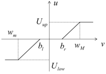
Fig. 1: Control input subject to dead zone and saturation.

The objective of this study is to develop an effective approach to enable the output $y$ to track the reference signal $r$ asymptotically under the following assumptions.

Assumption 1. The sign of input coefficient ${\mathop{\rm sgn}}(b)$ is known.

Assumption 2. The reference signal $r$ and its first $\left\lceil{\sum\nolimits_{i=1}^{j}{{\alpha_{i}}}}\right\rceil$-th order derivatives are piecewise continuous and bounded, $j=1,\cdots,n$.

There are three widely accepted definitions of fractional order derivative ${{\mathscr{D}}^{{\alpha}}}$, but the Caputo’s one is chosen for subsequent use due to some good properties, namely its derivative of constant equals zero and there’s no need to calculate fractional order derivative of initial value when operating Laplace transformation. The Caputo’s definition is

$$\textstyle{}_{c}{\mathscr{D}}_{t}^{\alpha}f\left(t\right)=\frac{1}{{\Gamma\left({m-\alpha}\right)}}\int_{c}^{t}{\frac{{{f^{\left(m\right)}}\left(\tau\right)}}{{{{\left({t-\tau}\right)}^{\alpha-m+1}}}}{\rm{d}}\tau},$$ (12)

where $m-1<\alpha<m,m\in\mathbb{N}^{+}$, $\Gamma\left(\alpha\right)=\int_{0}^{\infty}{{x^{\alpha-1}}{{\rm e}^{-x}}{\rm{d}}x}$ is the Gamma function.

On the basis of Caputo’s definition, the next additive law of exponents holds on condition that $f\left(c\right)=0$ and $0<p,q<1$

$${}_{c}{\mathscr{D}}_{t}^{p}\left({{}_{c}{\mathscr{D}}_{t}^{q}f\left(t\right)}\right)={{}_{c}{\mathscr{D}}_{t}^{q}\left({{}_{c}{\mathscr{D}}_{t}^{p}f\left(t\right)}\right)}={}_{c}{\mathscr{D}}_{t}^{p+q}f\left(t\right).$$ (13)

For purpose of convenient expression, the $\alpha$ order derivative from initial time zero ${}_{0}{\mathscr{D}}_{t}^{\alpha}$ is simplified as ${\mathscr{D}}^{\alpha}$. Just before uncovering the main results, some helpful lemmas need referring.

Lemma 1.

(see [41]) The differential equation ${{\mathscr{D}}^{\alpha}}y\left(t\right)=u\left(t\right)$ with fractional order $0<\alpha<1$, ${y\left(t\right)\in\mathbb{R}}$ and ${u\left(t\right)\in\mathbb{R}}$ can be transformed into the following linear continuous frequency distributed model

$$\left\{{\begin{array}[]{rl}\frac{{\partial z\left({\omega,t}\right)}}{{\partial t}}=&-\omega z\left({\omega,t}\right)+u\left(t\right),\\ y\left(t\right)=&\int_{0}^{\infty}{{\mu_{\alpha}}\left(\omega\right)z\left({\omega,t}\right){\rm{d}}\omega},\end{array}}\right.$$ (16)

where ${{\mu_{\alpha}}\left(\omega\right)={{{\omega^{-\alpha}}\sin\left({\alpha\pi}\right)}\mathord{\left/{\vphantom{{{\omega^{-\alpha}}\sin\left({\alpha\pi}\right)}\pi}}\right.\kern-1.2pt}\pi}}$ and $z\left({\omega,t}\right)\in\mathbb{R}$ is the true state of the system.

Remark 1.

The Lemma 1 implies the infinite dimension of fractional order state. And this lemma derives from zero initial condition, while the system response by definition of Riemann-Liouville or Caputo corresponds to the response of frequency distributed model with specific initial value [42]. With the help of equivalent frequency distributed model, the stability could be analyzed via Lyapunov technique where true sate replaces pseudo sate [43].

Lemma 2.

(see [44]) Supposing $r_{1}$ is the allowed maximum of control input $u(t)$ and $v(t)$ is the input signal to be differentiated with $\left|{{{\mathscr{D}}^{\alpha}}v\left(t\right)}\right|<\infty$, the following fractional order tracking differentiator (FOTD)

$$\left\{\begin{array}[]{l}{{\mathscr{D}}^{\alpha}}{x_{1}}\left(t\right)={x_{2}}\left(t\right),\\ {{\mathscr{D}}^{\alpha}}{x_{2}}\left(t\right)=u\left(t\right),\end{array}\right.$$ (19)

is convergent in the sense of ${x_{1}}(t)$ uniformly converging to $v(t)$ on $[0,\infty)$ as ${r_{1}}\to\infty$, and ${x_{2}}(t)$ is the general $\alpha$-th order differentiation of $v(t)$, where the control input $u\left(t\right)=-{r_{1}}{\rm{tanh}}({{x_{1}}\left(t\right)-v\left(t\right)+\frac{{{x_{2}}\left(t\right)\left|{{x_{2}}\left(t\right)}\right|}}{{{r_{1}}}}f\left(\alpha\right),{r_{2}}})$, ${r_{2}}>0$, $f\left(\alpha\right)=1-\frac{{{\Gamma^{2}}\left({\alpha+1}\right)}}{{\Gamma\left({2\alpha+1}\right)}}$ and $\tanh\left({z,\gamma}\right)=\frac{{{{\rm e}^{\gamma z}}-{{\rm e}^{-\gamma z}}}}{{{{\rm e}^{\gamma z}}+{{\rm e}^{-\gamma z}}}}$.

Remark 2.

In fact, the traditional integer order tracking differentiator could be regarded as a special case of the fractional order one [45]. Therefore, the fractional order derivative of signal will be obtained in time with required speed and smoothness by tuning parameters $r_{1}$ and $r_{2}$ of the FOTD as needed.

3 Main Results

A fractional order adaptive backstepping state feedback control method is unfolded in this section where two cases, known and unknown input coefficient, are studied separately. To deduce the main results smoothly, first of all, the controlled plant needs to undergo model transformation.

3.1 Model transformation

On the basis of following transformation

$$\left\{\begin{array}[]{l}{{\bar{x}}_{i}}={\delta_{i}}{x_{i}},i=1,\cdots,n,\\ {{\bar{\psi}}_{i}}\left({{x_{1}},\cdots,{x_{i}}}\right)={\delta_{i}}{\psi_{i}}\left({{x_{1}},\cdots,{x_{i}}}\right),i=1,\cdots,n,\\ {{\bar{\varphi}}_{i}}\left({{x_{1}},\cdots,{x_{i}}}\right)={\delta_{i}}{\varphi_{i}}\left({{x_{1}},\cdots,{x_{i}}}\right),i=1,\cdots,n,\\ {b^{\prime}}={\delta_{n}}b,\\ {d^{\prime}}={\delta_{n}}d,\end{array}\right.$$ (25)

with ${\delta_{1}}=1,~{}{\delta_{j}}=\prod\nolimits_{i=1}^{j-1}{d_{i}}~{}(j=2,\cdots,n)$. The controlled plant (5) will be changed into the system below

$$\left\{\begin{array}[]{rl}{{\mathscr{D}}^{{\alpha_{i}}}}{{\bar{x}}_{i}}=&{{\bar{x}}_{i+1}}+{{\bar{\psi}}_{i}}({x_{1}},\cdots,{x_{i}})\\ &+\bar{\varphi}_{i}^{\rm T}({x_{1}},\cdots,{x_{i}})\theta,~{}i=1,\cdots,n-1,\\ {{\mathscr{D}}^{{\alpha_{n}}}}{{\bar{x}}_{n}}=&{b^{\prime}}u(v)+{{\bar{\psi}}_{n}}(x)+\bar{\varphi}_{n}^{\rm T}(x)\theta+{d^{\prime}},\\ y=&{{\bar{x}}_{1}},\end{array}\right.$$ (30)

which is known as the normalized fractional order chain system.

Remark 3.

Considering the backstepping procedure, the general lower triangular FOS (5) needs converting into the normalized fractional order chain system (30) so that the FOABC method could be adopted. When the coefficients $d_{i}=1~{}(~{}i=1,\cdots,n-1~{})$, the controlled plant (5) reduces to the system (30) correspondingly.

3.2 Input decomposition

In order to deal with input saturation and dead zone, an intermediate variable $w$ is introduced between actual control input $u$ and desired control input $v$, namely, $u(v)=u[w(v)]$. Let $u(w)$ and $w(v)$ represent the dead zone nonlinearity and saturation nonlinearity, respectively, whereupon the previous control input restraint shown in Fig 1 is projected onto two directions as illustrated in Fig 2 where upper left and lower right represent input saturation and dead zone, respectively. It is obvious that though an intermediary is introduced, after the input $v$ mapped to $w$ and $w$ mapped to $u$, the final relationship between $v$ and $u$ has not changed. Therefore, the problem of control input restrained by input saturation and dead zone could be solved separately as shown in Fig 3.

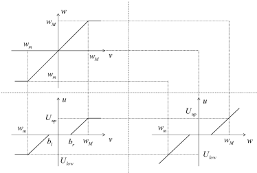
Fig. 2: The decomposition of control input.

Fig. 3: The intermediary $w$ between $v$ and $u$.

The expression in (11) will be taken apart as follows

$$w(v)=\left\{\begin{array}[]{cl}{w_{M}}&,~{}v(t)\geq{w_{M}}\\ v(t)&,~{}{w_{m}}\leq v(t)<{w_{M}}\\ {w_{m}}&,~{}v(t)<{w_{m}}\end{array}\right.$$ (34)

$$u(w)=\left\{\begin{array}[]{cl}m[w(v)-{b_{r}}]&,~{}w(v)\geq{b_{r}}\\ 0&,~{}{b_{l}}\leq w(v)<{b_{r}}\\ m[w(v)-{b_{l}}]&,~{}w(v)<{b_{l}}\end{array}\right.$$ (38)

The dead zone part (38) could be rewritten as

$$u(w)=mw(v)+d^{\prime\prime}(w),$$ (39)

where $d^{\prime\prime}(w)$ is a bounded term

$$d^{\prime\prime}(w)=\left\{\begin{array}[]{cl}-m{b_{r}}&,~{}w\geq{b_{r}}\\ -mw(v)&,~{}{b_{l}}\leq w<{b_{r}}\\ -m{b_{l}}&,~{}w<{b_{l}}\end{array}\right.$$ (43)

Then the last state equation of (30) changes correspondingly

$$\begin{array}[]{rl}{{\mathscr{D}}^{{\alpha_{n}}}}{{\bar{x}}_{n}}=&b^{\prime}u(v)+{{\bar{\psi}}_{n}}(x)+\bar{\varphi}_{n}^{\rm{T}}(x)\theta+d^{\prime}\\ =&b^{\prime}[mw(v)+d^{\prime\prime}(w)]+{{\bar{\psi}}_{n}}(x)+\bar{\varphi}_{n}^{\rm{T}}(x)\theta+d^{\prime}\\ =&\bar{b}w(v)+{{\bar{\psi}}_{n}}(x)+\bar{\varphi}_{n}^{\rm{T}}(x)\theta+\bar{d},\end{array}$$ (47)

where $\bar{b}=b^{\prime}m$, and $\bar{d}=d^{\prime}+b^{\prime}d^{\prime\prime}(w)$ is a disturbance-like term within unknown bound $\left|{\bar{d}}\right|\leq\bar{D}$. Finally, the system (30) will transform to

$$\left\{\begin{array}[]{rl}{{\mathscr{D}}^{{\alpha_{i}}}}{{\bar{x}}_{i}}=&{{\bar{x}}_{i+1}}+{{\bar{\psi}}_{i}}({x_{1}},\cdots,{x_{i}})\\ &+\bar{\varphi}_{i}^{\rm T}({x_{1}},\cdots,{x_{i}})\theta,~{}i=1,\cdots,n-1,\\ {{\mathscr{D}}^{{\alpha_{n}}}}{{\bar{x}}_{n}}=&{\bar{b}}w(v)+{{\bar{\psi}}_{n}}(x)+\bar{\varphi}_{n}^{\rm T}(x)\theta+{\bar{d}},\\ y=&{{\bar{x}}_{1}}.\end{array}\right.$$ (52)

The problem of dead zone and input saturation is transformed to the problem of input saturation and bounded disturbance at last.

It is noted that when either coefficient $b$ or slope $m$ is unknown, the parameter $\bar{b}$ will be unknown. In other words, the parameter $\bar{b}$ must be known under condition of known $b$ and $m$. In order to solve problem completely, both two cases will be studied afterwards.

3.3 FOABC with known $\bar{b}$

For the purpose of compensating saturation, a fractional order auxiliary system is designed to generate virtual signals $\lambda={[~{}{\lambda_{1}},{\lambda_{2}},\cdots,{\lambda_{n}}~{}]^{\rm T}}$ in the first place

$$\left\{\begin{array}[]{rl}{{\mathscr{D}}^{{\alpha_{i}}}}{\lambda_{i}}=&{\lambda_{i+1}}-{c_{i}}{\lambda_{i}},i=1,\cdots,n-1,\\ {{\mathscr{D}}^{{\alpha_{n}}}}{\lambda_{n}}=&\bar{b}\Delta w-{c_{n}}{\lambda_{n}},\end{array}\right.$$ (55)

where $\Delta w=w-v$, $c_{i}>1$ ($~{}i=2,3,\cdots,n-1$) and $c_{1},~{}c_{n}>0.5$.

Theorem 1.

Considering the plant (5) with known $\bar{b}$, there is a control method that consists of

the error variables

$$\left\{\begin{array}[]{l}{\varepsilon_{1}}={{\bar{x}}_{1}}-r-{\lambda_{1}},\\ {\varepsilon_{i}}={{\bar{x}}_{i}}-{{\mathscr{D}}^{\sum\limits_{j=1}^{i-1}{{\alpha_{j}}}}}r-{\tau_{i-1}}-{\lambda_{i}},~{}i=2,\cdots,n,\end{array}\right.$$ (58)

the stabilizing functions

$$\left\{\begin{array}[]{rl}{\tau_{1}}=&-{c_{1}}({{\bar{x}}_{1}}-r)-{{\bar{\psi}}_{1}}-\bar{\varphi}_{1}^{\rm T}\hat{\theta},\\ {\tau_{i}}=&-{c_{i}}({{\bar{x}}_{i}}-{{\mathscr{D}}^{\sum\limits_{j=1}^{i-1}{{\alpha_{j}}}}}r-{\tau_{i-1}})+{{\mathscr{D}}^{{\alpha_{i}}}}{\tau_{i-1}}\\ &-{{\bar{\psi}}_{i}}-\bar{\varphi}_{i}^{\rm T}\hat{\theta},~{}i=2,\cdots,n-1,\end{array}\right.$$ (62)

the parameter update law

$$\left\{\begin{array}[]{rl}{{\mathscr{D}}^{\beta}}\hat{\theta}=&\Lambda\sum\limits_{j=1}^{n}{{\varepsilon_{j}}{{\bar{\varphi}}_{j}}},\\ {{\mathscr{D}}^{\rho}}\hat{D}=&\xi\left|{{\varepsilon_{n}}}\right|,\end{array}\right.$$ (65)

the adaptive control law

$$\begin{array}[]{rl}v=&\frac{1}{{\bar{b}}}[-{c_{n}}{\varepsilon_{n}}+{{\mathscr{D}}^{\sum\limits_{j=1}^{n}{{\alpha_{j}}}}}r+{{\mathscr{D}}^{{\alpha_{n}}}}{\tau_{n-1}}-{{\bar{\psi}}_{n}}-\bar{\varphi}_{n}^{\rm{T}}\hat{\theta}\\ &-{\mathop{\rm sgn}}({\varepsilon_{n}})\hat{D}-{c_{n}}{\lambda_{n}}].\end{array}$$ (68)

Then all the signals in the closed-loop adaptive system are globally uniformly bounded, and the asymptotic tracking is achieved as

$$\mathop{\lim}\limits_{t\to\infty}[y(t)-r(t)]=0,$$ (69)

where $\hat{\theta}$ is the parameter estimate of $\theta$, $\hat{D}$ is the parameter estimate of $\bar{D}$, $\Lambda\in{{\mathbb{R}}^{q\times q}}$ is a positive definite matrix, $0<\beta,~{}\rho<1$ and $\xi>0$.

Proof.

Because of the uncertain $\theta$, the control method must perform the function of controller as well as estimator. If the ${\hat{\theta}}$ is regarded as the estimate of $\theta$, the estimated error $\tilde{\theta}=\theta-\hat{\theta}$ naturally forms and then the following equation is obtained in view of Caputo’s definition

$${{\mathscr{D}}^{\beta}}\tilde{\theta}={{\mathscr{D}}^{\beta}}\theta-{{\mathscr{D}}^{\beta}}\hat{\theta}=-{{\mathscr{D}}^{\beta}}\hat{\theta},$$ (70)

with the fractional order of update law $0<\beta<1$. Based on Lemma 1, (70) will be transformed into the frequency distributed model

$$\left\{\begin{array}[]{rl}\frac{{\partial{z_{\theta}}(\omega,t)}}{{\partial t}}=&-\omega{z_{\theta}}(\omega,t)-{{\mathscr{D}}^{\beta}}\hat{\theta},\\ \tilde{\theta}=&\int_{0}^{\infty}{{\mu_{\beta}}(\omega){z_{\theta}}(\omega,t){\rm d}\omega},\end{array}\right.$$ (73)

with ${z_{\theta}}(\omega,t)\in{{\mathbb{R}}^{q}}$ and ${\mu_{\beta}}{\rm{(}}\omega{\rm{)=}}\frac{{\sin(\beta\pi)}}{{{\omega^{\beta}}\pi}}$.

Step 1. Let’s begin with the first equation in (58) by calculating the fractional order derivative and introducing virtual control $\tau_{1}$

$$\begin{array}[]{rl}{{\mathscr{D}}^{{\alpha_{1}}}}{\varepsilon_{1}}=&{{\mathscr{D}}^{{\alpha_{1}}}}{{\bar{x}}_{1}}-{{\mathscr{D}}^{{\alpha_{1}}}}r-{{\mathscr{D}}^{{\alpha_{1}}}}{\lambda_{1}}\\ =&{{\bar{x}}_{2}}+{{\bar{\psi}}_{1}}+\bar{\varphi}_{1}^{\rm T}\theta-{{\mathscr{D}}^{{\alpha_{1}}}}r-{\lambda_{2}}+{c_{1}}{\lambda_{1}}\\ =&{\varepsilon_{2}}+{\tau_{1}}+{{\bar{\psi}}_{1}}+\bar{\varphi}_{1}^{\rm T}\theta+{c_{1}}{\lambda_{1}}.\end{array}$$ (77)

After transformation into the related frequency distributed model, the previous (77) will be

$$\left\{\begin{array}[]{rl}\frac{{\partial{z_{1}}(\omega,t)}}{{\partial t}}=&-\omega{z_{1}}(\omega,t)+{\varepsilon_{2}}+{\tau_{1}}\\ &+{{\bar{\psi}}_{1}}+\bar{\varphi}_{1}^{\rm T}\theta+{c_{1}}{\lambda_{1}},\\ {\varepsilon_{1}}=&\int_{0}^{\infty}{{\mu_{{\alpha_{1}}}}(\omega){z_{1}}(\omega,t){\rm d}\omega},\end{array}\right.$$ (81)

with ${\mu_{{\alpha_{1}}}}{\rm{(}}\omega{\rm{)=}}\frac{{\sin({\alpha_{1}}\pi)}}{{{\omega^{{\alpha_{1}}}}\pi}}$.

Selecting the Lyapunov function as

$$\begin{array}[]{rl}{V_{1}}=&\frac{1}{2}\int_{0}^{\infty}{{\mu_{\beta}}(\omega)z_{\theta}^{\rm T}(\omega,t){\Lambda^{-1}}{z_{\theta}}(\omega,t){\rm d}\omega}\\ &+\frac{1}{2}\int_{0}^{\infty}{{\mu_{{\alpha_{1}}}}(\omega)z_{1}^{2}(\omega,t){\rm d}\omega},\end{array}$$ (84)

then its derivative is expressed as

$$\begin{array}[]{rl}{\dot{V}_{1}}=&-\int_{0}^{\infty}{\omega{\mu_{\beta}}(\omega)z_{\theta}^{\rm T}(\omega,t){\Lambda^{-1}}{z_{\theta}}(\omega,t){\rm d}\omega}\\ &-\int_{0}^{\infty}{\omega{\mu_{{\alpha_{1}}}}(\omega)z_{1}^{2}(\omega,t){\rm d}\omega}-{\tilde{\theta}^{\rm T}}{\Lambda^{-1}}{{\mathscr{D}}^{\beta}}\hat{\theta}\\ &+{\varepsilon_{1}}({\varepsilon_{2}}+{\tau_{1}}+{\bar{\psi}_{1}}+\bar{\varphi}_{1}^{\rm T}\theta+{c_{1}}{\lambda_{1}}).\end{array}$$ (88)

Designing the stabilizing function ${\tau_{1}}$ as (62), the resulting derivative is

$$\begin{array}[]{rl}{{\dot{V}}_{1}}=&-\int_{0}^{\infty}{\omega{\mu_{\beta}}(\omega)z_{\theta}^{\rm T}(\omega,t){\Lambda^{-1}}{z_{\theta}}(\omega,t){\rm d}\omega}\\ &-\int_{0}^{\infty}{\omega{\mu_{{\alpha_{1}}}}(\omega)z_{1}^{2}(\omega,t){\rm d}\omega}\\ &+{{\tilde{\theta}}^{\rm T}}({\varepsilon_{1}}{{\bar{\varphi}}_{1}}-{\Lambda^{-1}}{{\mathscr{D}}^{\beta}}\hat{\theta})-{c_{1}}\varepsilon_{1}^{2}+{\varepsilon_{1}}{\varepsilon_{2}}\\ \leq&-\int_{0}^{\infty}{\omega{\mu_{\beta}}(\omega)z_{\theta}^{\rm T}(\omega,t){\Lambda^{-1}}{z_{\theta}}(\omega,t){\rm d}\omega}\\ &-\int_{0}^{\infty}{\omega{\mu_{{\alpha_{1}}}}(\omega)z_{1}^{2}(\omega,t){\rm d}\omega}\\ &+{{\tilde{\theta}}^{\rm T}}({\varepsilon_{1}}{{\bar{\varphi}}_{1}}-{\Lambda^{-1}}{{\mathscr{D}}^{\beta}}\hat{\theta})-{{\bar{c}}_{1}}\varepsilon_{1}^{2}{\rm{+}}\frac{1}{2}\varepsilon_{2}^{2},\end{array}$$ (95)

where ${\bar{c}_{1}}={c_{1}}-\frac{1}{2}>0$.

If ${\varepsilon_{2}}=0$ and ${{\mathscr{D}}^{\beta}}\hat{\theta}=\Lambda{\varepsilon_{1}}{{\bar{\varphi}}_{1}}$, then ${\varepsilon_{1}}$ and ${\tilde{\theta}}$ are both asymptotically convergent to zero in accordance with LaSalle invariance principle [46].

Step $i(i=2,\cdots,n-1).$ We continue to investigate the $i$-th equation of (58) with the introduction of virtual control variable $\tau_{i}$, then the differential of $\varepsilon_{i}$ is

$$\begin{array}[]{rl}{{\mathscr{D}}^{{\alpha_{i}}}}{\varepsilon_{i}}=&{{\mathscr{D}}^{{\alpha_{i}}}}{{\bar{x}}_{i}}-{{\mathscr{D}}^{\sum\limits_{j=1}^{i}{{\alpha_{j}}}}}r-{{\mathscr{D}}^{{\alpha_{i}}}}{\tau_{i-1}}-{{\mathscr{D}}^{{\alpha_{i}}}}{\lambda_{i}}\\ =&{{\bar{x}}_{i+1}}+{{\bar{\psi}}_{i}}+\bar{\varphi}_{i}^{\rm T}\theta-{{\mathscr{D}}^{\sum\limits_{j=1}^{i}{{\alpha_{j}}}}}r-{{\mathscr{D}}^{{\alpha_{i}}}}{\tau_{i-1}}\\ &-{\lambda_{i+1}}+{c_{i}}{\lambda_{i}}\\ =&{\varepsilon_{i+1}}+{\tau_{i}}+{{\bar{\psi}}_{i}}+\bar{\varphi}_{i}^{\rm T}\theta-{{\mathscr{D}}^{{\alpha_{i}}}}{\tau_{i-1}}+{c_{i}}{\lambda_{i}}.\end{array}$$ (100)

Its frequency distributed model is shown below

$$\left\{\begin{array}[]{rl}\frac{{\partial{z_{i}}(\omega,t)}}{{\partial t}}=&-\omega{z_{i}}(\omega,t)+{\varepsilon_{i+1}}+{\tau_{i}}+{{\bar{\psi}}_{i}}+\bar{\varphi}_{i}^{\rm T}\theta\\ &-{{\mathscr{D}}^{{\alpha_{i}}}}{\tau_{i-1}}+{c_{i}}{\lambda_{i}},\\ {\varepsilon_{i}}=&\int_{0}^{\infty}{{\mu_{{\alpha_{i}}}}(\omega){z_{i}}(\omega,t){\rm d}\omega},\end{array}\right.$$ (104)

with ${\mu_{{\alpha_{i}}}}{\rm{(}}\omega{\rm{)=}}\frac{{\sin({\alpha_{i}}\pi)}}{{{\omega^{{\alpha_{i}}}}\pi}}$.

This step aims at stabilizing the system (104) through Lyapunov function below

$${V_{i}}={V_{i-1}}+\frac{1}{2}\int_{0}^{\infty}{{\mu_{{\alpha_{i}}}}\left(\omega\right)z_{i}^{2}\left({\omega,t}\right){\rm{d}}\omega}.$$ (105)

By calculating the derivative of $V_{i}$

$$\begin{array}[]{rl}{{\dot{V}}_{i}}=&{{\dot{V}}_{i-1}}-\int_{0}^{\infty}{\omega{\mu_{{\alpha_{i}}}}(\omega)z_{i}^{2}(\omega,t){\rm d}\omega}\\ &+{\varepsilon_{i}}({\varepsilon_{i+1}}+{\tau_{i}}+{{\bar{\psi}}_{i}}+\bar{\varphi}_{i}^{\rm T}\theta-{{\mathscr{D}}^{{\alpha_{i}}}}{\tau_{i-1}}+{c_{i}}{\lambda_{i}})\\ \leq&-\int_{0}^{\infty}{\omega{\mu_{\beta}}(\omega)z_{\theta}^{\rm T}(\omega,t){\Lambda^{-1}}{z_{\theta}}(\omega,t){\rm d}\omega}\\ &-\sum\limits_{j=1}^{i}{\int_{0}^{\infty}{\omega{\mu_{{\alpha_{j}}}}(\omega)z_{j}^{2}(\omega,t){\rm d}\omega}}\\ &+{{\tilde{\theta}}^{\rm T}}(\sum\limits_{j=1}^{i-1}{{\varepsilon_{j}}{{\bar{\varphi}}_{j}}}-{\Lambda^{-1}}{{\mathscr{D}}^{\beta}}\hat{\theta})-\sum\limits_{j=1}^{i-1}{{{\bar{c}}_{j}}\varepsilon_{j}^{2}}+\frac{1}{2}\varepsilon_{i}^{2}\\ &+{\varepsilon_{i}}({\varepsilon_{i+1}}+{\tau_{i}}+{{\bar{\psi}}_{i}}+\bar{\varphi}_{i}^{\rm T}\theta-{{\mathscr{D}}^{{\alpha_{i}}}}{\tau_{i-1}}+{c_{i}}{\lambda_{i}}),\end{array}$$ (112)

and designing the stabilizing function $\tau_{i}$ as (62), we further infer the derivative $\dot{V}_{i}$

$$\begin{array}[]{rl}{{\dot{V}}_{i}}\leq&-\int_{0}^{\infty}{\omega{\mu_{\beta}}(\omega)z_{\theta}^{\rm T}(\omega,t){\Lambda^{-1}}{z_{\theta}}(\omega,t){\rm d}\omega}\\ &-\sum\limits_{j=1}^{i}{\int_{0}^{\infty}{\omega{\mu_{{\alpha_{j}}}}(\omega)z_{j}^{2}(\omega,t){\rm d}\omega}}\\ &+{{\tilde{\theta}}^{\rm T}}(\sum\limits_{j=1}^{i}{{\varepsilon_{j}}{{\bar{\varphi}}_{j}}}-{\Lambda^{-1}}{{\mathscr{D}}^{\beta}}\hat{\theta})-\sum\limits_{j=1}^{i-1}{{{\bar{c}}_{j}}\varepsilon_{j}^{2}}\\ &+\frac{1}{2}\varepsilon_{i}^{2}-{c_{i}}\varepsilon_{i}^{2}+{\varepsilon_{i}}{\varepsilon_{i+1}}\\ \leq&-\int_{0}^{\infty}{\omega{\mu_{\beta}}(\omega)z_{\theta}^{\rm T}(\omega,t){\Lambda^{-1}}{z_{\theta}}(\omega,t){\rm d}\omega}\\ &-\sum\limits_{j=1}^{i}{\int_{0}^{\infty}{\omega{\mu_{{\alpha_{j}}}}(\omega)z_{j}^{2}(\omega,t){\rm d}\omega}}\\ &+{{\tilde{\theta}}^{\rm T}}(\sum\limits_{j=1}^{i}{{\varepsilon_{j}}{{\bar{\varphi}}_{j}}}-{\Lambda^{-1}}{{\mathscr{D}}^{\beta}}\hat{\theta})-\sum\limits_{j=1}^{i}{{{\bar{c}}_{j}}\varepsilon_{j}^{2}}+\frac{1}{2}\varepsilon_{i+1}^{2},\end{array}$$ (120)

where ${{\bar{c}}_{i}}={c_{i}}-1>0$.

Indeed, when $\varepsilon_{i+1}=0$ and ${{\mathscr{D}}^{\beta}}\hat{\theta}=\Lambda\sum\limits_{j=1}^{i}{{\varepsilon_{j}}{{\bar{\varphi}}_{j}}}$, then $\varepsilon_{i}$ is asymptotically convergent to zero. While $\varepsilon_{i}=0$, the update law $\Lambda\sum\limits_{j=1}^{i}{{\varepsilon_{j}}{{\bar{\varphi}}_{j}}}$ reduces to $\Lambda\sum\limits_{j=1}^{i{\rm{-}}1}{{\varepsilon_{j}}{{\bar{\varphi}}_{j}}}$, which returns to step $i-1.$

Step $n.$ It is not until the last step that the real control input $v$ finally turns up, hence the whole system will be under control as adaptive control law design finishes. Before the last design, however, there is a disturbance-like term with unknown bound $\bar{D}$ worthy of attention. If the ${\hat{D}}$ is regarded as the estimate of $\bar{D}$, the estimated error will be $\tilde{D}=\bar{D}-\hat{D}$, and then the following equation is obtained in view of Caputo’s definition

$${{\mathscr{D}}^{\rho}}\tilde{D}={{\mathscr{D}}^{\rho}}\bar{D}-{{\mathscr{D}}^{\rho}}\hat{D}=-{{\mathscr{D}}^{\rho}}\hat{D},$$ (121)

with the fractional order of update law $0<\rho<1$. Based on Lemma 1, (121) will be transformed into the frequency distributed model

$$\left\{\begin{array}[]{rl}\frac{{\partial{z_{D}}(\omega,t)}}{{\partial t}}=&-\omega{z_{D}}(\omega,t)-{{\mathscr{D}}^{\rho}}\hat{D},\\ \tilde{D}=&\int_{0}^{\infty}{{\mu_{\rho}}(\omega){z_{D}}(\omega,t){\rm{d}}\omega},\end{array}\right.$$ (124)

with ${\mu_{\rho}}{\rm{(}}\omega{\rm{)=}}\frac{{\sin(\rho\pi)}}{{{\omega^{\rho}}\pi}}$.

Similar to the previous steps, the error variable $\varepsilon_{n}$ will be derived based on the equation (58), subsequently its differential function comes out

$$\begin{array}[]{rl}{{\mathscr{D}}^{{\alpha_{n}}}}{\varepsilon_{n}}=&{{\mathscr{D}}^{{\alpha_{n}}}}{{\bar{x}}_{n}}-{{\mathscr{D}}^{\sum\limits_{j=1}^{n}{{\alpha_{j}}}}}r-{{\mathscr{D}}^{{\alpha_{n}}}}{\tau_{n-1}}-{{\mathscr{D}}^{{\alpha_{n}}}}{\lambda_{n}}\\ =&\bar{b}w(v)+{{\bar{\psi}}_{n}}+\bar{\varphi}_{n}^{\rm{T}}\theta+\bar{d}-{{\mathscr{D}}^{\sum\limits_{j=1}^{n}{{\alpha_{j}}}}}r\\ &-{{\mathscr{D}}^{{\alpha_{n}}}}{\tau_{n-1}}-\bar{b}\Delta w+{c_{n}}{\lambda_{n}}\\ =&\bar{b}v+{{\bar{\psi}}_{n}}+\bar{\varphi}_{n}^{\rm{T}}\theta+\bar{d}-{{\mathscr{D}}^{\sum\limits_{j=1}^{n}{{\alpha_{j}}}}}r\\ &-{{\mathscr{D}}^{{\alpha_{n}}}}{\tau_{n-1}}+{c_{n}}{\lambda_{n}}.\end{array}$$ (130)

The frequency distributed model is

$$\left\{\begin{array}[]{rl}\frac{{\partial{z_{n}}(\omega,t)}}{{\partial t}}=&-\omega{z_{n}}(\omega,t)+\bar{b}v+{{\bar{\psi}}_{n}}+\bar{\varphi}_{n}^{\rm{T}}\theta\\ &+\bar{d}-{{\mathscr{D}}^{\sum\limits_{j=1}^{n}{{\alpha_{j}}}}}r-{{\mathscr{D}}^{{\alpha_{n}}}}{\tau_{n-1}}+{c_{n}}{\lambda_{n}},\\ {\varepsilon_{n}}=&\int_{0}^{\infty}{{\mu_{{\alpha_{n}}}}(\omega){z_{n}}(\omega,t){\rm{d}}\omega},\end{array}\right.$$ (134)

with ${\mu_{{\alpha_{n}}}}{\rm{(}}\omega{\rm{)=}}\frac{{\sin({\alpha_{n}}\pi)}}{{{\omega^{{\alpha_{n}}}}\pi}}$.

With the purpose of ensuring ${\varepsilon_{n}}\to 0$ as $t\to\infty$, the last and overall Lyapunov function is decided

$$\begin{array}[]{rl}{V_{n}}=&{V_{n-1}}+\frac{1}{2}\int_{0}^{\infty}{{\mu_{{\alpha_{n}}}}(\omega)z_{n}^{2}(\omega,t){\rm d}\omega}\\ &+\frac{1}{{2\xi}}\int_{0}^{\infty}{{\mu_{\rho}}(\omega)z_{D}^{2}(\omega,t){\rm{d}}\omega}.\end{array}$$ (137)

By adopting the inequality we induce in the step $n-1$, the derivative of (137) is

$$\begin{array}[]{rl}{{\dot{V}}_{n}}=&{{\dot{V}}_{n-1}}-\int_{0}^{\infty}{\omega{\mu_{{\alpha_{n}}}}(\omega)z_{n}^{2}(\omega,t){\rm{d}}\omega}\\ &-\frac{1}{\xi}\int_{0}^{\infty}{\omega{\mu_{\rho}}(\omega)z_{D}^{2}(\omega,t){\rm{d}}\omega}+{\varepsilon_{n}}(\bar{b}v+{{\bar{\psi}}_{n}}\\ &+\bar{\varphi}_{n}^{\rm{T}}\theta+\bar{d}-{{\mathscr{D}}^{\sum\limits_{j=1}^{n}{{\alpha_{j}}}}}r-{{\mathscr{D}}^{{\alpha_{n}}}}{\tau_{n-1}}+{c_{n}}{\lambda_{n}})\\ &-\frac{1}{\xi}\tilde{D}{{\mathscr{D}}^{\rho}}\hat{D}\\ \leq&-\int_{0}^{\infty}{\omega{\mu_{\beta}}(\omega)z_{\theta}^{\rm{T}}(\omega,t){\Lambda^{-1}}{z_{\theta}}(\omega,t){\rm{d}}\omega}\\ &-\sum\limits_{j=1}^{n}{\int_{0}^{\infty}{\omega{\mu_{{\alpha_{j}}}}(\omega)z_{j}^{2}(\omega,t){\rm{d}}\omega}}\\ &-\frac{1}{\xi}\int_{0}^{\infty}{\omega{\mu_{\rho}}(\omega)z_{D}^{2}(\omega,t){\rm{d}}\omega}-\sum\limits_{j=1}^{n-1}{{{\bar{c}}_{j}}\varepsilon_{j}^{2}}+\frac{1}{2}\varepsilon_{n}^{2}\\ &+{{\tilde{\theta}}^{\rm{T}}}(\sum\limits_{j=1}^{n-1}{{\varepsilon_{j}}{{\bar{\varphi}}_{j}}}-{\Lambda^{-1}}{{\mathscr{D}}^{\beta}}\hat{\theta})+{\varepsilon_{n}}(\bar{b}v+{{\bar{\psi}}_{n}}\\ &+\bar{\varphi}_{n}^{\rm{T}}\theta+\bar{d}-{{\mathscr{D}}^{\sum\limits_{j=1}^{n}{{\alpha_{j}}}}}r-{{\mathscr{D}}^{{\alpha_{n}}}}{\tau_{n-1}}+{c_{n}}{\lambda_{n}})\\ &-\frac{1}{\xi}\tilde{D}{{\mathscr{D}}^{\rho}}\hat{D}.\end{array}$$ (148)

Designing the adaptive control law $v$ as (68), the simplified derivative $\dot{V}_{n}$ is

$$\begin{array}[]{rl}{{\dot{V}}_{n}}\leq&-\int_{0}^{\infty}{\omega{\mu_{\beta}}(\omega)z_{\theta}^{\rm{T}}(\omega,t){\Lambda^{-1}}{z_{\theta}}(\omega,t){\rm{d}}\omega}\\ &-\sum\limits_{j=1}^{n}{\int_{0}^{\infty}{\omega{\mu_{{\alpha_{j}}}}(\omega)z_{j}^{2}(\omega,t){\rm{d}}\omega}}\\ &-\frac{1}{\xi}\int_{0}^{\infty}{\omega{\mu_{\rho}}(\omega)z_{D}^{2}(\omega,t){\rm{d}}\omega}-\sum\limits_{j=1}^{n-1}{{{\bar{c}}_{j}}\varepsilon_{j}^{2}}+\frac{1}{2}\varepsilon_{n}^{2}\\ &+{{\tilde{\theta}}^{\rm{T}}}(\sum\limits_{j=1}^{n}{{\varepsilon_{j}}{{\bar{\varphi}}_{j}}}-{\Lambda^{-1}}{{\mathscr{D}}^{\beta}}\hat{\theta})-{c_{n}}\varepsilon_{n}^{2}+{\varepsilon_{n}}\bar{d}\\ &-\left|{{\varepsilon_{n}}}\right|\hat{D}-\frac{1}{\xi}\tilde{D}{{\mathscr{D}}^{\rho}}\hat{D}.\end{array}$$ (154)

Because of the following inequality

$$\begin{array}[]{rl}{\varepsilon_{n}}\bar{d}-\left|{{\varepsilon_{n}}}\right|\hat{D}\leq\left|{{\varepsilon_{n}}}\right|\bar{D}-\left|{{\varepsilon_{n}}}\right|\hat{D}=\tilde{D}\left|{{\varepsilon_{n}}}\right|,\end{array}$$ (156)

and the the parameter update law ${{\mathscr{D}}^{\beta}}\hat{\theta},~{}{{\mathscr{D}}^{\rho}}\hat{D}$ (65), the $\dot{V}_{n}$ is

$$\begin{array}[]{rl}\dot{V}_{n}\leq&-\int_{0}^{\infty}{\omega{\mu_{\beta}}(\omega)z_{\theta}^{\rm{T}}(\omega,t){\Lambda^{-1}}{z_{\theta}}(\omega,t){\rm{d}}\omega}\\ &-\sum\limits_{j=1}^{n}{\int_{0}^{\infty}{\omega{\mu_{{\alpha_{j}}}}(\omega)z_{j}^{2}(\omega,t){\rm{d}}\omega}}\\ &-\frac{1}{\xi}\int_{0}^{\infty}{\omega{\mu_{\rho}}(\omega)z_{D}^{2}(\omega,t){\rm{d}}\omega}-\sum\limits_{j=1}^{n}{{{\bar{c}}_{j}}\varepsilon_{j}^{2}},\end{array}$$ (160)

where ${{\bar{c}}_{n}}={c_{n}}-\frac{1}{2}>0$.

According to the LaSalle invariant principle, the $z_{i}(\omega,t)$ are convergent to the zero point, which makes the error variables $\varepsilon_{i}$ convergent to zero. Moreover, as the input of constructed system (55), the error $\Delta w$ has nothing to do with error variables $\varepsilon_{i}$, thus the controller design will not be influenced by $\Delta w$ and the boundedness of estimation will be guaranteed [47]. ∎

In the recursive procedure of controllers design, every coefficient $c_{i}$ is required to be greater than a certain constant with the purpose of establishing inequality and eliminating the product ${\varepsilon_{i}}{\varepsilon_{i+1}}$. This procedure leads to the conservatism of application, though relatively superior control performance will be realized afterwards. To meet the different needs of practice, a more general and flexible FOABC strategy is derived from Theorem 1.

Corollary 1.

For the purpose of compensation, a fractional order auxiliary system is designed to generate virtual signals $\lambda={[~{}{\lambda_{1}},{\lambda_{2}},\cdots,{\lambda_{n}}~{}]^{\rm T}}$

$$\left\{\begin{array}[]{rl}{{\mathscr{D}}^{{\alpha_{i}}}}{\lambda_{i}}=&{\lambda_{i+1}}-{a_{i}}{\mathop{\rm sgn}}({\lambda_{i}}){\left|{{\lambda_{i}}}\right|^{{\mu_{i}}}},i=1,\cdots,n-1,\\ {{\mathscr{D}}^{{\alpha_{n}}}}{\lambda_{n}}=&\bar{b}\Delta w-{a_{n}}{\mathop{\rm sgn}}({\lambda_{n}}){\left|{{\lambda_{n}}}\right|^{{\mu_{n}}}}.\end{array}\right.$$ (163)

There is a control method that consists of

the error variables

$$\left\{\begin{array}[]{l}{\varepsilon_{1}}={{\bar{x}}_{1}}-r-{\lambda_{1}},\\ {\varepsilon_{i}}={{\bar{x}}_{i}}-{{\mathscr{D}}^{\sum\limits_{j=1}^{i-1}{{\alpha_{j}}}}}r-{\tau_{i-1}}-{\lambda_{i}},~{}i=2,\cdots,n,\end{array}\right.$$ (166)

the stabilizing functions

$$\left\{\begin{array}[]{rl}{\tau_{1}}=&-{c_{1}}{\mathop{\rm sgn}}({\varepsilon_{1}}){\left|{{\varepsilon_{1}}}\right|^{{\sigma_{1}}}}-{{\bar{\psi}}_{1}}-\bar{\varphi}_{1}^{\rm T}\hat{\theta}\\ &-{a_{1}}{\mathop{\rm sgn}}({\lambda_{1}}){\left|{{\lambda_{1}}}\right|^{{\mu_{1}}}},\\ {\tau_{i}}=&-{\varepsilon_{i-1}}-{c_{i}}{\mathop{\rm sgn}}({\varepsilon_{i}}){\left|{{\varepsilon_{i}}}\right|^{{\sigma_{i}}}}-{{\bar{\psi}}_{i}}-\bar{\varphi}_{i}^{\rm T}\hat{\theta}\\ &+{{\mathscr{D}}^{{\alpha_{i}}}}{\tau_{i-1}}-{a_{i}}{\mathop{\rm sgn}}({\lambda_{i}}){\left|{{\lambda_{i}}}\right|^{{\mu_{i}}}},\\ &i=2,\cdots,n-1,\end{array}\right.$$ (172)

the parameter update law

$$\left\{\begin{array}[]{rl}{{\mathscr{D}}^{\beta}}\hat{\theta}=&\Lambda\sum\limits_{j=1}^{n}{{\varepsilon_{j}}{{\bar{\varphi}}_{j}}},\\ {{\mathscr{D}}^{\rho}}\hat{D}=&\xi\left|{{\varepsilon_{n}}}\right|,\end{array}\right.$$ (175)

the adaptive control law

$$\begin{array}[]{rl}v=&\frac{1}{{\bar{b}}}[-{\varepsilon_{n-1}}-{c_{n}}{\mathop{\rm sgn}}({\varepsilon_{n}}){\left|{{\varepsilon_{n}}}\right|^{{\sigma_{n}}}}-{{\bar{\psi}}_{n}}-\bar{\varphi}_{n}^{\rm{T}}\hat{\theta}\\ &-{\mathop{\rm sgn}}({\varepsilon_{n}})\hat{D}+{{\mathscr{D}}^{\sum\limits_{j=1}^{n}{{\alpha_{j}}}}}r+{{\mathscr{D}}^{{\alpha_{n}}}}{\tau_{n-1}}\\ &-{a_{n}}{\mathop{\rm sgn}}({\lambda_{n}}){\left|{{\lambda_{n}}}\right|^{{\mu_{n}}}}].\end{array}$$ (179)

Then all the signals in the closed-loop adaptive system are globally uniformly bounded, and the asymptotic tracking is achieved as

$$\mathop{\lim}\limits_{t\to\infty}[y(t)-r(t)]=0,$$ (180)

where $\hat{\theta}$ is the parameter estimate of $\theta$, $\hat{D}$ is the parameter estimate of $\bar{D}$, $\Lambda\in{{\mathbb{R}}^{q\times q}}$ is a positive definite matrix, $a_{i},c_{i},\xi>0$, $0<\rho,\beta,\alpha_{i},\sigma_{i},\mu_{i}<1~{}(i=1,\cdots,n)$ and $\Delta w=w-v$.

The proof of Corollary 1 is omitted here, because one can easily complete it according to the procedure of Theorem 1.

3.4 FOABC with unknown $\bar{b}$

Last subsection discusses about the FOABC under the condition of known $\bar{b}$, while the unknown case is common and more complicated. For example, when the slope $m$ or input coefficient $b$ is unknown, $\bar{b}=\delta_{n}bm$ will be unknown as well and an alternative FOABC method without known $\bar{b}$ is expected.

For the purpose of compensation, a fractional order auxiliary system is designed to generate virtual signals $\lambda={[~{}{\lambda_{1}},{\lambda_{2}},\cdots,{\lambda_{n}}~{}]^{\rm T}}$ in the first place

$$\left\{\begin{array}[]{l}{{\mathscr{D}}^{{\alpha_{i}}}}{\lambda_{i}}={\lambda_{i+1}}-{c_{i}}{\lambda_{i}},i=1,\cdots,n-1,\\ {{\mathscr{D}}^{{\alpha_{n}}}}{\lambda_{n}}=\frac{1}{{\hat{p}}}\Delta w-{c_{n}}{\lambda_{n}},\end{array}\right.$$ (183)

where ${\hat{p}}$ is the estimate of $\frac{1}{{\bar{b}}}$, $\Delta w=w-v$, $c_{i}>1$ ($~{}i=2,3,\cdots,n-1$) and $c_{1},~{}c_{n}>0.5$.

Theorem 2.

Considering the plant (5) with known ${\rm sgn}(b)$, there is a control method that consists of

the error variables

$$\left\{\begin{array}[]{l}{\varepsilon_{1}}={{\bar{x}}_{1}}-r-{\lambda_{1}},\\ {\varepsilon_{i}}={{\bar{x}}_{i}}-{{\mathscr{D}}^{\sum\limits_{j=1}^{i-1}{{\alpha_{j}}}}}r-{\tau_{i-1}}-{\lambda_{i}},~{}i=2,\cdots,n,\end{array}\right.$$ (186)

the stabilizing functions

$$\left\{\begin{array}[]{rl}{\tau_{1}}=&-{c_{1}}({{\bar{x}}_{1}}-r)-{{\bar{\psi}}_{1}}-\bar{\varphi}_{1}^{\rm T}\hat{\theta},\\ {\tau_{i}}=&-{c_{i}}({{\bar{x}}_{i}}-{{\mathscr{D}}^{\sum\limits_{j=1}^{i-1}{{\alpha_{j}}}}}r-{\tau_{i-1}})+{{\mathscr{D}}^{{\alpha_{i}}}}{\tau_{i-1}}-{{\bar{\psi}}_{i}}\\ &-\bar{\varphi}_{i}^{\rm T}\hat{\theta},~{}i=2,\cdots,n-1,\end{array}\right.$$ (190)

the parameter update law

$$\left\{\begin{array}[]{l}{{\mathscr{D}}^{\beta}}\hat{\theta}=\Lambda\sum\limits_{j=1}^{n}{{\varepsilon_{j}}{{\bar{\varphi}}_{j}}},\\ {{\mathscr{D}}^{\gamma}}\hat{p}=-\eta{\mathop{\rm sgn}}(\bar{b}){\varepsilon_{n}}\bar{w},\\ {{\mathscr{D}}^{\rho}}\hat{D}=\xi\left|{{\varepsilon_{n}}}\right|,\end{array}\right.$$ (194)

the adaptive control law

$$\left\{\begin{array}[]{rl}v=&\hat{p}\bar{v},\\ \bar{v}=&-{c_{n}}{\lambda_{n}}-{c_{n}}{\varepsilon_{n}}-{\mathop{\rm sgn}}({\varepsilon_{n}})\hat{D}+{{\mathscr{D}}^{\sum\limits_{j=1}^{n}{{\alpha_{j}}}}}r\\ &+{{\mathscr{D}}^{{\alpha_{n}}}}{\tau_{n-1}}-{{\bar{\psi}}_{n}}-{{\bar{\varphi}}^{\rm T}_{n}}\hat{\theta}.\end{array}\right.$$ (198)

Then all the signals in the closed-loop adaptive system are globally uniformly bounded, and the asymptotic tracking is achieved as

$$\mathop{\lim}\limits_{t\to\infty}[y(t)-r(t)]=0,$$ (199)

where $\hat{p}$ is the parameter estimate of $p=\frac{1}{{\bar{b}}}$, $\hat{\theta}$ is the parameter estimate of $\theta$, $\hat{D}$ is the parameter estimate of $\bar{D}$, $\Lambda\in{{\mathbb{R}}^{q\times q}}$ is a positive definite matrix, $0<\gamma,~{}\beta,~{}\rho<1$, $\eta,\xi>0$ and $w=\hat{p}\bar{w}$.

Proof.

Since the difference between known $\bar{b}$ and unknown $\bar{b}$ only depends on the last state equation (5), the first $n-1$ steps in this theorem are identical to the proof of Theorem 1, thus they are omitted here in case of repetitive work. Due to the introduction of an unknown parameter $\bar{b}$, we first design a new estimator that regards $\hat{p}$ as the estimate of $p=1/\bar{b}$ and ${\tilde{p}}=p-\hat{p}$ as the relevant estimated error. Note that

$${{\mathscr{D}}^{\gamma}}\tilde{p}={{\mathscr{D}}^{\gamma}}p-{{\mathscr{D}}^{\gamma}}\hat{p}=-{{\mathscr{D}}^{\gamma}}\hat{p},$$ (200)

with the fractional order of update law $0<\gamma<1$. Its frequency distributed model is analogous to (73) and (124) which could be written as

$$\left\{\begin{array}[]{rl}\frac{{\partial{z_{p}}(\omega,t)}}{{\partial t}}=&-\omega{z_{p}}(\omega,t)-{{\mathscr{D}}^{\gamma}}\hat{p},\\ \tilde{p}=&\int_{0}^{\infty}{{\mu_{\gamma}}(\omega){z_{p}}(\omega,t){\rm d}\omega},\end{array}\right.$$ (203)

with ${\mu_{\gamma}}{\rm{(}}\omega{\rm{)=}}\frac{{\sin(\gamma\pi)}}{{{\omega^{\gamma}}\pi}}$.

With the definition of

$$\left\{\begin{array}[]{l}w=\hat{p}\bar{w},\\ v=\hat{p}\bar{v},\end{array}\right.$$ (206)

then we have

$$\begin{array}[]{r}\bar{b}w-\frac{1}{{\hat{p}}}\Delta w=\bar{w}-\bar{b}\tilde{p}\bar{w}-(\bar{w}-\bar{v})=\bar{v}-\bar{b}\tilde{p}\bar{w}.\end{array}$$ (208)

The derivative of $\varepsilon_{n}$ is

$$\begin{array}[]{rl}{{\mathscr{D}}^{{\alpha_{n}}}}{\varepsilon_{n}}=&{{\mathscr{D}}^{{\alpha_{n}}}}{{\bar{x}}_{n}}-{{\mathscr{D}}^{\sum\limits_{j=1}^{n}{{\alpha_{j}}}}}r-{{\mathscr{D}}^{{\alpha_{n}}}}{\tau_{n-1}}-{{\mathscr{D}}^{{\alpha_{n}}}}{\lambda_{n}}\\ =&\bar{b}w+{{\bar{\psi}}_{n}}+\bar{\varphi}_{n}^{\rm{T}}\theta+\bar{d}-{{\mathscr{D}}^{\sum\limits_{j=1}^{n}{{\alpha_{j}}}}}r\\ &-{{\mathscr{D}}^{{\alpha_{n}}}}{\tau_{n-1}}-\frac{1}{{\hat{p}}}\Delta w+{c_{n}}{\lambda_{n}}\\ =&\bar{v}-\bar{b}\tilde{p}\bar{w}+{{\bar{\psi}}_{n}}+\bar{\varphi}_{n}^{\rm{T}}\theta+\bar{d}-{{\mathscr{D}}^{\sum\limits_{j=1}^{n}{{\alpha_{j}}}}}r\\ &-{{\mathscr{D}}^{{\alpha_{n}}}}{\tau_{n-1}}+{c_{n}}{\lambda_{n}}.\end{array}$$ (214)

It’s corresponding frequency distributed model is

$$\left\{\begin{array}[]{rl}\frac{{\partial{z_{n}}(\omega,t)}}{{\partial t}}=&-\omega{z_{n}}(\omega,t)+\bar{v}-\bar{b}\tilde{p}\bar{w}+{{\bar{\psi}}_{n}}+\bar{\varphi}_{n}^{\rm{T}}\theta\\ &+\bar{d}-{{\mathscr{D}}^{\sum\limits_{j=1}^{n}{{\alpha_{j}}}}}r-{{\mathscr{D}}^{{\alpha_{n}}}}{\tau_{n-1}}+{c_{n}}{\lambda_{n}},\\ {\varepsilon_{n}}=&\int_{0}^{\infty}{{\mu_{{\alpha_{n}}}}(\omega){z_{n}}(\omega,t){\rm{d}}\omega},\end{array}\right.$$ (218)

with ${\mu_{{\alpha_{n}}}}{\rm{(}}\omega{\rm{)=}}\frac{{\sin({\alpha_{n}}\pi)}}{{{\omega^{{\alpha_{n}}}}\pi}}$.

Selecting the Lyapunov function

$$\begin{array}[]{rl}{V_{n}}=&{V_{n-1}}+\frac{1}{2}\int_{0}^{\infty}{{\mu_{{\alpha_{n}}}}(\omega)z_{n}^{2}(\omega,t){\rm{d}}\omega}\\ &+\frac{{\left|{\bar{b}}\right|}}{{2\eta}}\int_{0}^{\infty}{{\mu_{\gamma}}(\omega)z_{p}^{2}(\omega,t){\rm{d}}\omega}\\ &+\frac{1}{{2\xi}}\int_{0}^{\infty}{{\mu_{\rho}}(\omega)z_{D}^{2}(\omega,t){\rm{d}}\omega},\end{array}$$ (222)

and adopting the preceding derivative $\dot{V}_{n-1}$, the derivative of $V_{n}$ is

$$\begin{array}[]{rl}{{\dot{V}}_{n}}=&{{\dot{V}}_{n-1}}-\int_{0}^{\infty}{\omega{\mu_{{\alpha_{n}}}}(\omega)z_{n}^{2}(\omega,t){\rm{d}}\omega}\\ &-\frac{{\left|{\bar{b}}\right|}}{\eta}\int_{0}^{\infty}{\omega{\mu_{\gamma}}(\omega)z_{p}^{2}(\omega,t){\rm{d}}\omega}\\ &-\frac{1}{\xi}\int_{0}^{\infty}{\omega{\mu_{\rho}}(\omega)z_{D}^{2}(\omega,t){\rm{d}}\omega}+{\varepsilon_{n}}(-\bar{b}\tilde{p}\bar{w}+{{\bar{\psi}}_{n}}\\ &+\bar{\varphi}_{n}^{\rm{T}}\theta+\bar{d}-{{\mathscr{D}}^{\sum\limits_{j=1}^{n}{{\alpha_{j}}}}}r-{{\mathscr{D}}^{{\alpha_{n}}}}{\tau_{n-1}}+\bar{v}+{c_{n}}{\lambda_{n}})\\ &-\frac{{\left|{\bar{b}}\right|}}{\eta}\tilde{p}{{\mathscr{D}}^{\gamma}}\hat{p}-\frac{1}{\xi}\tilde{D}{{\mathscr{D}}^{\rho}}\hat{D}\\ \leq&-\sum\limits_{j=1}^{n}{\int_{0}^{\infty}{\omega{\mu_{{\alpha_{j}}}}(\omega)z_{j}^{2}(\omega,t){\rm{d}}\omega}}\\ &-\int_{0}^{\infty}{\omega{\mu_{\beta}}(\omega)z_{\theta}^{\rm{T}}(\omega,t){\Lambda^{-1}}{z_{\theta}}(\omega,t){\rm{d}}\omega}\\ &-\frac{{\left|{\bar{b}}\right|}}{\eta}\int_{0}^{\infty}{\omega{\mu_{\gamma}}(\omega)z_{p}^{2}(\omega,t){\rm{d}}\omega}\\ &-\frac{1}{\xi}\int_{0}^{\infty}{\omega{\mu_{\rho}}(\omega)z_{D}^{2}(\omega,t){\rm{d}}\omega}\\ &-\sum\limits_{j=1}^{n-1}{{{\bar{c}}_{j}}\varepsilon_{j}^{2}}+\frac{1}{2}\varepsilon_{n}^{2}-\tilde{p}\left|{\bar{b}}\right|[\frac{1}{\eta}{{\mathscr{D}}^{\gamma}}\hat{p}+{\varepsilon_{n}}{\mathop{\rm sgn}}(\bar{b})\bar{w}]\\ &+{{\tilde{\theta}}^{\rm{T}}}(\sum\limits_{j=1}^{n}{{\varepsilon_{j}}{{\bar{\varphi}}_{j}}}-{\Lambda^{-1}}{{\mathscr{D}}^{\beta}}\hat{\theta})+{\varepsilon_{n}}[{{\bar{\psi}}_{n}}+\bar{\varphi}_{n}^{\rm{T}}\hat{\theta}\\ &+{\mathop{\rm sgn}}({\varepsilon_{n}})\hat{D}-{{\mathscr{D}}^{\sum\limits_{j=1}^{n}{{\alpha_{j}}}}}r-{{\mathscr{D}}^{{\alpha_{n}}}}{\tau_{n-1}}+\bar{v}\\ &+{c_{n}}{\lambda_{n}}]+{\varepsilon_{n}}\bar{d}-\left|{{\varepsilon_{n}}}\right|\hat{D}-\frac{1}{\xi}\tilde{D}{{\mathscr{D}}^{\rho}}\hat{D}.\end{array}$$ (236)

Taking the parameter update law (194) and adaptive control law (198) into account, the above derivative $\dot{V}_{n}$ will be simplified

$$\begin{array}[]{rl}{{\dot{V}}_{n}}\leq&-\sum\limits_{j=1}^{n}{\int_{0}^{\infty}{\omega{\mu_{{\alpha_{j}}}}(\omega)z_{j}^{2}(\omega,t){\rm{d}}\omega}}\\ &-\int_{0}^{\infty}{\omega{\mu_{\beta}}(\omega)z_{\theta}^{\rm{T}}(\omega,t){\Lambda^{-1}}{z_{\theta}}(\omega,t){\rm{d}}\omega}\\ &-\frac{{\left|{\bar{b}}\right|}}{\eta}\int_{0}^{\infty}{\omega{\mu_{\gamma}}(\omega)z_{p}^{2}(\omega,t){\rm{d}}\omega}\\ &-\frac{1}{\xi}\int_{0}^{\infty}{\omega{\mu_{\rho}}(\omega)z_{D}^{2}(\omega,t){\rm{d}}\omega}-\sum\limits_{j=1}^{n}{{{\bar{c}}_{j}}\varepsilon_{j}^{2}},\end{array}$$ (241)

where ${{\bar{c}}_{n}}={c_{n}}-\frac{1}{2}>0$.

Based on the LaSalle invariant principle, the error variable $\varepsilon_{i}$ are convergent to zero by the similar proof of Theorem 1, which establishes Theorem 2. ∎

Just like Theorem 1, in the recursive procedure of controllers design, every coefficient $c_{i}$ is required to be greater than a certain constant with the purpose of establishing inequality and eliminating the product ${\varepsilon_{i}}{\varepsilon_{i+1}}$. This procedure also leads to the conservatism of application, though relatively superior control performance will be realized afterwards. To meet the different needs of control, a more general and flexible FOABC strategy is derived from Theorem 2 and Corollary 1.

Corollary 2.

For the purpose of compensation, a fractional order auxiliary system is designed to generate virtual signals $\lambda={[~{}{\lambda_{1}},{\lambda_{2}},\cdots,{\lambda_{n}}~{}]^{\rm T}}$

$$\left\{\begin{array}[]{rl}{{\mathscr{D}}^{{\alpha_{i}}}}{\lambda_{i}}=&{\lambda_{i+1}}-{a_{i}}{\mathop{\rm sgn}}({\lambda_{i}}){\left|{{\lambda_{i}}}\right|^{{\mu_{i}}}},\\ &i=1,\cdots,n-1,\\ {{\mathscr{D}}^{{\alpha_{n}}}}{\lambda_{n}}=&\frac{1}{{\hat{p}}}\Delta w-{a_{n}}{\mathop{\rm sgn}}({\lambda_{n}}){\left|{{\lambda_{n}}}\right|^{{\mu_{n}}}}.\end{array}\right.$$ (245)

There is a control method that consists of

the error variables

$$\left\{\begin{array}[]{l}{\varepsilon_{1}}={{\bar{x}}_{1}}-r-{\lambda_{1}},\\ {\varepsilon_{i}}={{\bar{x}}_{i}}-{{\mathscr{D}}^{\sum\limits_{j=1}^{i-1}{{\alpha_{j}}}}}r-{\tau_{i-1}}-{\lambda_{i}},~{}i=2,\cdots,n,\end{array}\right.$$ (248)

the stabilizing functions

$$\left\{\begin{array}[]{rl}{\tau_{1}}=&-{c_{1}}{\mathop{\rm sgn}}({\varepsilon_{1}}){\left|{{\varepsilon_{1}}}\right|^{{\sigma_{1}}}}-{{\bar{\psi}}_{1}}-\bar{\varphi}_{1}^{\rm T}\hat{\theta}\\ &-{a_{1}}{\mathop{\rm sgn}}({\lambda_{1}}){\left|{{\lambda_{1}}}\right|^{{\mu_{1}}}},\\ {\tau_{i}}=&-{\varepsilon_{i-1}}-{c_{i}}{\mathop{\rm sgn}}({\varepsilon_{i}}){\left|{{\varepsilon_{i}}}\right|^{{\sigma_{i}}}}-{{\bar{\psi}}_{i}}-\bar{\varphi}_{i}^{\rm T}\hat{\theta}\\ &+{{\mathscr{D}}^{{\alpha_{i}}}}{\tau_{i-1}}-{a_{i}}{\mathop{\rm sgn}}({\lambda_{i}}){\left|{{\lambda_{i}}}\right|^{{\mu_{i}}}},\\ &i=2,\cdots,n-1,\end{array}\right.$$ (254)

the parameter update law

$$\left\{\begin{array}[]{l}{{\mathscr{D}}^{\beta}}\hat{\theta}=\Lambda\sum\limits_{j=1}^{n}{{\varepsilon_{j}}{{\bar{\varphi}}_{j}}},\\ {{\mathscr{D}}^{\gamma}}\hat{p}=-\eta{\mathop{\rm sgn}}(\bar{b}){\varepsilon_{n}}\bar{w},\\ {{\mathscr{D}}^{\rho}}\hat{D}=\xi\left|{{\varepsilon_{n}}}\right|,\end{array}\right.$$ (258)

the adaptive control law

$$\left\{\begin{array}[]{rl}v=&\hat{p}\bar{v},\\ \bar{v}=&-{\varepsilon_{n-1}}-{c_{n}}{\mathop{\rm sgn}}({\varepsilon_{n}}){\left|{{\varepsilon_{n}}}\right|^{{\sigma_{n}}}}-{\mathop{\rm sgn}}({\varepsilon_{n}})\hat{D}\\ &+{{\mathscr{D}}^{\sum\limits_{j=1}^{n}{{\alpha_{j}}}}}r+{{\mathscr{D}}^{{\alpha_{n}}}}{\tau_{n-1}}-{{\bar{\psi}}_{n}}-\bar{\varphi}_{n}^{\rm{T}}\hat{\theta}\\ &-{a_{n}}{\mathop{\rm sgn}}({\lambda_{n}}){\left|{{\lambda_{n}}}\right|^{{\mu_{n}}}}.\end{array}\right.$$ (263)

Then all the signals in the closed-loop adaptive system are globally uniformly bounded, and the asymptotic tracking is achieved as

$$\mathop{\lim}\limits_{t\to\infty}[y(t)-r(t)]=0,$$ (264)

where $\hat{p}$ is the parameter estimate of $\frac{1}{{\bar{b}}}$, $\hat{\theta}$ is the parameter estimate of $\theta$, $\hat{D}$ is the parameter estimate of $\bar{D}$, $\Lambda\in{{\mathbb{R}}^{q\times q}}$ is a positive definite matrix, $0<\gamma,\beta,\rho,\alpha_{i},\sigma_{i},\mu_{i}<1$ , $\eta,\xi,a_{i},c_{i}>0~{}(i=1,\cdots,n)$, $w=\hat{p}\bar{w}$ and $\Delta w=w-v$.

The proof of Corollary 2 is omitted as well, since one can easily complete it according to the procedure of Theorem 2.

The proposed theorems and corollaries provide a new and original approach that the control input subject to saturation and dead zone could be coped with separately. By applying adaptive backstepping control strategy, the controller design is completed in the procedure of proof afterwards. To highlight the characteristics and advantages of the proposed control strategy clearly, the following remark is presented here, which is also part of our contributions.

Remark 4.

There are four additional innovations needing emphasis.

• With the introduction of intermediate variable $w$ and projection, the control input subject to nonsmooth nonlinear dead zone and saturation is decomposed into two independent parts. The desired input $v$ goes through saturation part and changes into intermediate variable $w$, then $w$ changes into the actual input $u$ after dead zone part. As the bounded disturbance $d^{\prime}$ combines with a bounded term $d^{\prime\prime}$ of dead zone part, the disturbance-like term forms, and finally, the problem of dead zone and saturation is transformed into that of disturbance and saturation. It is worth mentioning that when the $\bar{b}$ is unknown, the slope of input $m$ may be also unknown, that is, all parameters of input nonsmooth nonlinearities are unknown, but our proposed method still works according to Theorem 2 and Corollary 2. As far as we known, there isn’t any similar solution to dead zone and saturation no matter whether the object is fractional order or not.

• In Corollary 1 and Corollary 2, instead of establishing the inequality just as Theorem 1 and Theorem 2, the product ${\varepsilon_{i}}{\varepsilon_{i+1}}$ is eliminated directly by adding the error variables ${\varepsilon_{i}}$ into the stabilizing functions $\tau_{i}$ and the adaptive control law $v$, which reduces the restraint of coefficients $c_{i}$. Compared with the traditional linear feedback elements ${c_{i}}{\varepsilon_{i}}$ and ${c_{i}}{\lambda_{i}}$, the nonlinear elements ${c_{i}}{\mathop{\rm sgn}}({\varepsilon_{i}}){\left|{{\varepsilon_{i}}}\right|^{{\sigma_{i}}}}$ and ${a_{i}}{\mathop{\rm sgn}}({\lambda_{i}}){\left|{{\lambda_{i}}}\right|^{{\mu_{i}}}}$ bring some advantages, namely larger error corresponds to smaller gain, but smaller error gives larger gain, which requires smaller control cost and reduces overshoot caused by sudden change of reference signal. In addition, controllers design will enjoy more degree of freedom since new parameters are introduced.

• The theorems and corollaries realize tracking and compensate the nonlinearities of incommensurate FOS. If $\alpha_{i}=\alpha$ these methods change into the commensurate case. Furthermore, if $\alpha=1$, the above theories will be common solutions to integer order systems with nonsmooth nonlinearities. When reference signal equals zero $r=0$, the tracking task turns into a stabilizing task.

• Instead of fractional order derivative of the Lyapunov function [39, 40], indirect Lyapunov method with frequency distributed model is adopted so that the order of the parameter update law is no longer fixed to the system order. Its design enjoys more degree of freedom and it is expected to achieve better control performance. By setting the order $\beta$ and $\gamma$ equal to the integer, the update law changes back.

4 Simulation Study

Numerical simulations will be carried out in this section with the piecewise numerical approximation algorithm [23]. The specific form of controlled plant is chosen as

$$\left\{\begin{array}[]{l}{{\mathscr{D}}^{0.5}}{x_{1}}=2{x_{2}}-0.5x_{1}^{2}+{x_{1}}\theta,\\ {{\mathscr{D}}^{0.6}}{x_{2}}=-{x_{3}}+\frac{{{x_{2}}-x_{2}^{3}}}{{1+x_{1}^{4}}}-\sin\left({{x_{1}}}\right)\theta,\\ {{\mathscr{D}}^{0.7}}{x_{3}}=bu(v)-{{\rm{e}}^{-x_{1}^{2}}}\sin\left({5{x_{3}}}\right)+\cos\left({{x_{1}}}\right)\theta+d,\end{array}\right.$$ (268)

with the unknown constant $\theta=0.1$, bounded disturbance $d={\rm cos}(\pi t)+{\rm sin}(3t)$, possibly unknown control input coefficient $b=3$, the unknown parameters of nonsmooth nonlinearities $U_{up}=1.8$, $U_{low}=-1.5$, $b_{r}=0.8$, $b_{l}=-0.5$ and possibly unknown slope $m=1$. A sinusoidal signal $r(t)={\rm{sin}}(2t)$ is set to reference signal and will be tracked by the output of the system with initial state $x(0)=\left[~{}0.3,~{}-0.4,~{}~{}0.2~{}\right]^{\rm{T}}$. The FOTD could be configured as required, here $r_{1}=50,r_{2}=5$, by which the fractional order derivative of stabilizing function $\tau_{i}$ and reference signal $r$ , like ${\mathscr{D}}^{\alpha_{i}}\tau_{i-1}$ and ${{\mathscr{D}}^{\sum\nolimits_{j=1}^{i-1}{{\alpha_{j}}}}}r$, will be obtained easily. The $\rm{tanh}(\cdot)$ takes place of $\rm{sgn}(\cdot)$ in control law $v$ for smooth calculation and chattering rejection.

To demonstrate the applicability of FOABC method, the system (268) with or without the certainty of $b$ and $m$ will be both investigated, and results are presented in Example 1 and Example 2, respectively.

Example 1. Supposing the coefficient $\bar{b}$ of the system (268) is known, the case 1 adopts the method of Theorem 1, the case 2 adopts the method of Corollary 1, and the case 3 is only carried out with the general FOABC method [37] where no solution is provided for nonsmooth nonlinearities. Selecting the controller parameters $c_{1}=c_{2}=c_{3}=a_{1}=a_{2}=a_{3}=4$, $\sigma_{1}=\sigma_{2}=\sigma_{3}=\mu_{1}=\mu_{2}=\mu_{3}=0.8$, $\rho=\beta=0.9$, $\xi=\Lambda=1$ and the initial parameter estimates $\hat{D}(0)=\hat{\theta}(0)=0$, then we view $\varepsilon(t)=r(t)-y(t)$ as tracking error and obtain the tracking performance shown in Fig. 4. Meanwhile, the Fig. 5 and Fig. 6 present the corresponding estimations $\hat{\theta}$ and $\hat{D}$, respectively. The actual control input is drawn in Fig. 7.

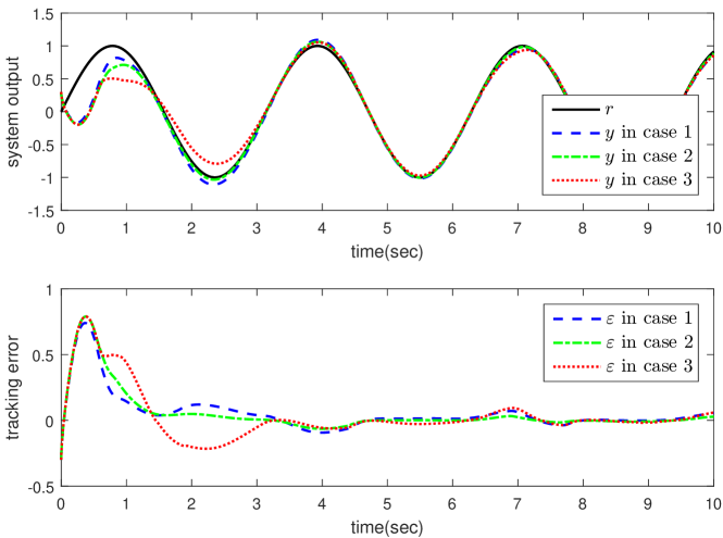
Fig. 4: The performance of tracking in Example 1.

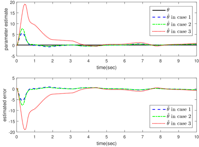
Fig. 5: The estimation of $\theta$ in Example 1.

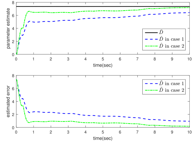
Fig. 6: The relevant estimation of $\bar{D}$ in Example 1.

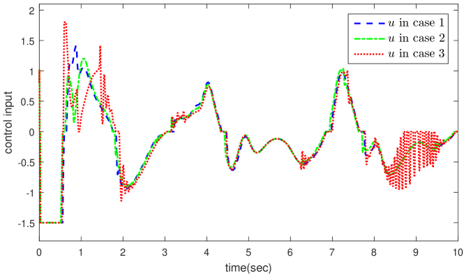
Fig. 7: The needed control input in Example 1.

The output $y(t)$, in view of the Fig. 4, could track the reference signal $r(t)$ for all three cases. However, compared with the case 2 and case 3, the case 1 shows better tracking result, because the inequality and restraint of coefficient make the Lyapunov function stricter and more conservative. Besides better tracking performance, the parameter estimation also shows the superiority. Although there is a larger tracking error at the beginning, the output of case 2 also converges to reference signal more quickly than that of case 3. And case 2 shows similar superiority of parameter estimation, too. Compared with the method of case 1, the controllers design of case 2 enjoys more degree of freedom, which may meet the different needs of practical project. For quantitative comparison, some details are calculated as Table 1.

Table 1: The control performance of Example 1

	$||{\varepsilon(t)}||_{\rm{max}}$	$||{\varepsilon(t)}||_{2}$	$||\tilde{\theta}(t)||_{2}$	$||\tilde{D}(t)||_{2}$	$||{u(t)}||_{2}$
case 1	0.73965	18.084	114.58	245.41	67.604
case 2	0.78887	19.639	145.80	154.38	64.233
case 3	0.78892	23.036	514.81	$\backslash$	67.396

Since the disturbance hasn’t been considered in the controlled plant of general FOABC method [37], it is short of ability to estimate $\bar{D}$, which results in no data in Fig. 6 and Table 1.

Example 2. Supposing the coefficient $\bar{b}$ of the system (268) is unknown, the Example 2 will be executed by the same parameters as Example 1 except $\gamma=0.9$, $\hat{p}(0)=0.01$ and $\eta=1$. Because $\hat{p}$ will be regarded as denominator during the calculation, the initial value $\hat{p}(0)$ cannot be equal to zero. The case 1 adopts the method of Theorem 2. The case 2 adopts the method of Corollary 2. The case 3 is only carried out with the general FOABC method [37] which will be compared with our method shown in case 1 and case 2. The curves of output and tracking error are drawn on Fig. 8. As for estimation, Fig. 9, Fig. 10 and Fig. 11 express the the parameter estimate of $\theta$, $p$ and $\bar{D}$, respectively. The synergetic control input is shown in Fig. 12.

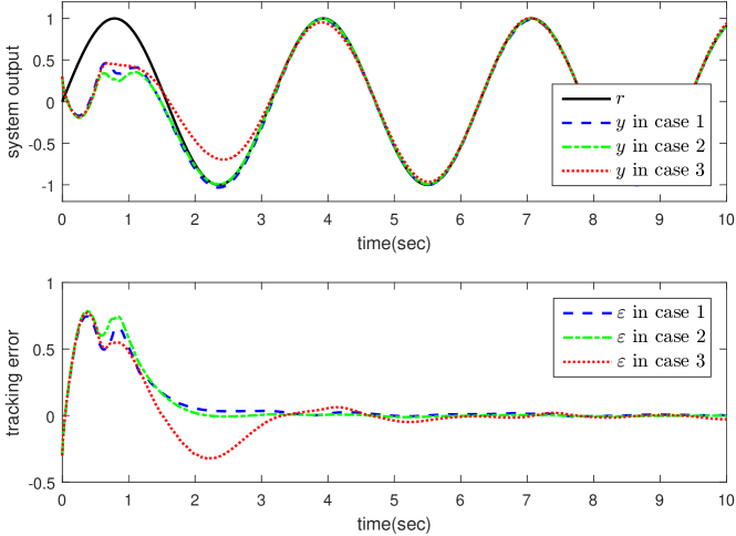
Fig. 8: The performance of tracking in Example 2.

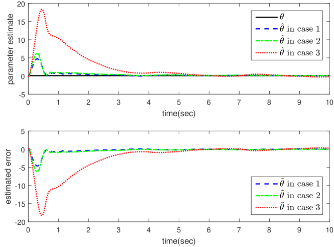
Fig. 9: The estimation of $\theta$ in Example 2.

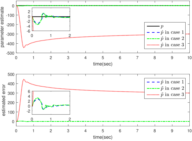
Fig. 10: The relevant estimation of $p$ in Example 2.

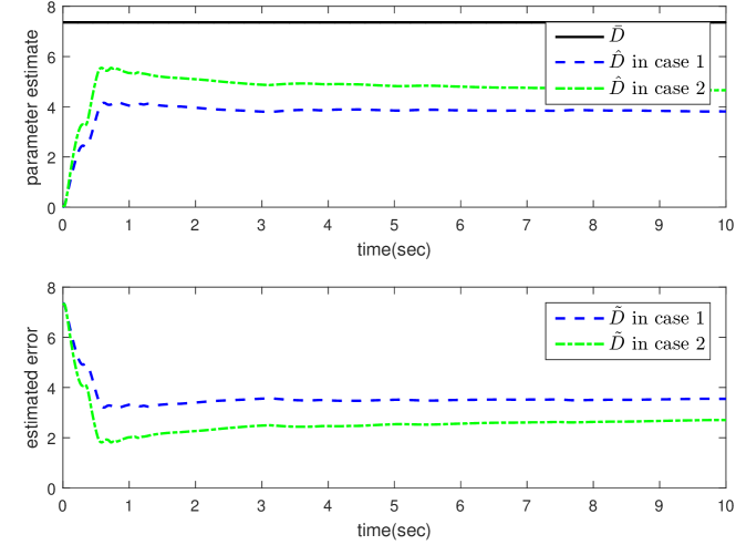
Fig. 11: The relevant estimation of $\bar{D}$ in Example 2.

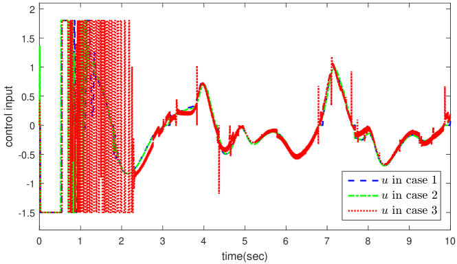
Fig. 12: The needed control input in Example 2.

The tracking performance in this example, analogous to Example 1, exposes the high speed of our methods that output could keep pace with the reference signal rapidly. What’s more, our estimating procedure illustrates that the methods we suggest have excellent advantage. The case 1 still shows its superiority for the same reason as Example 1. The controllers of case 2 also enjoys more freedom. Some details are also calculated as Table 2.

Table 2: The control performance of Example 2

	$||{\varepsilon(t)}||_{\rm{max}}$	$||{\varepsilon(t)}||_{2}$	$||{\tilde{\theta}(t)}||_{2}$	$||{\tilde{p}(t)}||_{2}$	$||{\tilde{D}(t)}||_{2}$	$||{u(t)}||_{2}$
case 1	0.74547	39.939	116.67	209.591	2193.7	227.30
case 2	0.78489	43.165	161.70	205.557	1599.4	225.35
case 3	0.77238	55.456	1007.3	199644	$\backslash$	230.88

As can be observed from Table 1 and Table 2, compared with the system with known coefficient, the unknown case needs more control cost in the same circumstances of simulation, but only gets barely satisfactory tracking performance. Compared with the case 1, the case 2 requires less control cost because of the nonlinear feedback element.

The Example 2 proceeds under the condition of unknown $\bar{b}$. Because of $\bar{b}=\delta_{n}bm$, the $b$ or $m$ is uncertain, too. That is to say, our proposed method still works well without prior knowledge of all parameters of nonsmooth nonlinearities, namely unknown $m$, $U_{up}$, $U_{low}$, $b_{r}$ and $b_{l}$. Therefore, it leads to higher versatility and wider application.

5 Conclusions

The input saturation and dead zone of uncertain nonlinear FOS are investigated in this paper. After the decomposition of control input, the problem of input saturation and dead zone is transformed into the problem of input saturation and bounded disturbance, which could be solved in accordance with FOABC. It is the first time that scholars have studied the FOS with input saturation and dead zone at the same time. What’s more, our proposed method could still work even if all parameters of these nonsmooth nonlinearities are unknown. It is believed that this novel method provides a new way to cope with control input subject to saturation and dead zone.

References

References

- Zhou and Wen [2008] Zhou, J., Wen, C.Y.. Adaptive Backstepping Control of Uncertain Systems: Nonsmooth Nonlinearities, Interactions or Time-variations. Berlin: Springer; 2008.
- Zuo et al. [2015] Zuo, Z.Y., Li, X., Shi, Z.G.. adaptive control of uncertain gear transmission servo systems with deadzone nonlinearity. ISA Transactions 2015;58:67–75.
- Zuo et al. [2016] Zuo, Z.Y., Ju, X.L., Ding, Z.T.. Control of gear transmission servo systems with asymmetric deadzone nonlinearity. IEEE Transactions on Control System Technology 2016;24(4):1472–1479.
- Xu et al. [2016] Xu, B., Su, Q., Zhang, J.H., Lu, Z.Y.. Analysis and compensation for the cascade dead-zones in the proportional control valve. ISA Transactions 2016;Doi: 10.1016/j.isatra.2016.10.012.
- Liu et al. [2013] Liu, L., Liu, Y.J., Chen, C.L.P.. Adaptive neural network control for a DC motor system with dead-zone. Nonlinear Dynamics 2013;72(1):141–147.
- Jiang et al. [2015] Jiang, Y.M., Liu, Z., Chen, C., Zhang, Y.. Adaptive robust fuzzy control for dual arm robot with unknown input deadzone nonlinearity. Nonlinear Dynamics 2015;81(3):1301–1314.
- Xu [2015] Xu, B.. Robust adaptive neural control of flexible hypersonic flight vehicle with dead-zone input nonlinearity. Nonlinear Dynamics 2015;80(3):1509–1520.
- Carnevale and Astolfi [2014] Carnevale, D., Astolfi, A.. Semi-global multi-frequency estimation in the presence of deadzone and saturation. IEEE Transactions on Automatic Control 2014;59(7):1913–1918.
- Shen et al. [2016] Shen, Q.K., Shi, P., Shi, Y., Zhang, J.H.. Adaptive output consensus with saturation and dead-zone and its application. IEEE Transactions on Industrial Electronics 2016;Doi: 10.1109/TIE.2016.2587858.
- Chen et al. [2012a] Chen, J., Wang, X.P., Ding, R.F.. Gradient based estimation algorithm for Hammerstein systems with saturation and dead-zone nonlinearities. Applied Mathematical Modelling 2012a;36(1):238–243.
- Chen et al. [2012b] Chen, J., Lu, X.L., Ding, R.F.. Gradient-based iterative algorithm for Wiener systems with saturation and dead-zone nonlinearities. Journal of Vibration and Control 2012b;20(4):634–640.
- Chen et al. [2016a] Chen, Y.Q., Wei, Y.H., Liang, S., Wang, Y.. Indirect model reference adaptive control for a class of fractional order systems. Communications in Nonlinear Science and Numerical Simulation 2016a;39:458–471.
- Du et al. [2016] Du, B., Wei, Y.H., Liang, S., Wang, Y.. Estimation of exact initial states of fractional order systems. Nonlinear Dynamics 2016;86(3):2061–2070.
- Yin et al. [2014] Yin, C., Chen, Y.Q., Zhong, S.M.. Fractional-order sliding mode based extremum seeking control of a class of nonlinear systems. Automatica 2014;50(12):3173–3181.
- Chen et al. [2016b] Chen, Y.Q., Wei, Y.H., Zhong, H., Wang, Y.. Sliding mode control with a second-order switching law for a class of nonlinear fractional order systems. Nonlinear Dynamics 2016b;85(1):633–643.
- Li et al. [2009] Li, Y., Chen, Y.Q., Podlubny, I.. Mittag-Leffler stability of fractional order nonlinear dynamic systems. Automatica 2009;45(8):1965–1969.
- Lu and Chen [2010] Lu, J.G., Chen, Y.Q.. Robust stability and stabilization of fractional-order interval systems with the fractional order : the case. IEEE Transactions on Automatic Control 2010;55(1):152–158.
- Li and Wang [2012] Li, C., Wang, J.C.. Robust stability and stabilization of fractional order interval systems with coupling relationships: the case. Journal of the Franklin Institute 2012;349(7):2406–2419.
- Shen and Lam [2016] Shen, J., Lam, J.. Stability and performance analysis for positive fractional-order systems with time-varying delays. IEEE Transactions on Automatic Control 2016;61(9):2676–2681.
- Yan [2011] Yan, Z.M.. Controllability of fractional-order partial neutral functional integrodifferential inclusions with infinite delay. Journal of the Franklin Institute 2011;348(8):2156–2173.
- Acharya et al. [2014] Acharya, A., Das, S., Pan, I., Das, S.. Extending the concept of analog Butterworth filter for fractional order systems. Signal Processing 2014;94:409–420.
- Wei et al. [2016a] Wei, Y.H., Tse, P.W., Du, B., Wang, Y.. An innovative fixed-pole numerical approximation for fractional order systems. ISA Transactions 2016a;62:94–102.
- Wei et al. [2014] Wei, Y.H., Gao, Q., Peng, C., Wang, Y.. A rational approximate method to fractional order systems. International Journal of Control Automation & Systems 2014;12(6):1180–1186.
- Sheng et al. [2011] Sheng, H., Li, Y., Chen, Y.Q.. Application of numerical inverse laplace transform algorithms in fractional calculus. Journal of the Franklin Institute 2011;348(2):315–330.
- Petráš et al. [2012] Petráš, I., Sierociuk, D., Podlubny, I.. Identification of parameters of a half-order system. IEEE Transactions on Signal Processing 2012;60(10):5561–5566.
- Hu et al. [2016] Hu, Y.S., Fan, Y., Wei, Y.H., Wang, Y., Liang, Q.. Subspace-based continuous-time identification of fractional order systems from non-uniformly sampled data. International Journal of Systems Science 2016;47(1):122–134.
- Luo and Chen [2012] Luo, Y., Chen, Y.Q.. Stabilizing and robust fractional order PI controller synthesis for first order plus time delay systems. Automatica 2012;48(9):2159–2167.
- Machado [1997] Machado, J.A.T.. Analysis and design of fractional-order digital control systems. Systems Analysis Modelling Simulation 1997;27:107–122.
- Lim et al. [2013] Lim, Y.H., Oh, K.K., Ahn, H.S.. Stability and stabilization of fractional-order linear systems subject to input saturation. IEEE Transactions on Automatic Control 2013;58(4):1062–1067.
- Shahri et al. [2015] Shahri, E.S.A., Alfi, A., Machado, J.A.T.. An extension of estimation of domain of attraction for fractional order linear system subject to saturation control. Applied Mathematics Letters 2015;47:26–34.
- Shahri and Balochian [2015] Shahri, E.S.A., Balochian, S.. Analysis of fractional-order linear systems with saturation using Lyapunov’s second method and convex optimization. International Journal of Automation & Computing 2015;12(4):440–447.
- Luo [2014] Luo, J.H.. State-feedback control for fractional-order nonlinear systems subject to input saturation. Mathematical Problems in Engineering 2014;DOI: 10.1155/2014/891639.
- Abooee and Haeri [2013] Abooee, A., Haeri, M.. Stabilisation of commensurate fractional-order polytopic non-linear differential inclusion subject to input non-linearity and unknown disturbances. IET Control Theory & Applications 2013;7(12):1624–1633.
- Tian and Fei [2014] Tian, X.M., Fei, S.M.. Robust control of a class of uncertain fractional-order chaotic systems with input nonlinearity via an adaptive sliding mode technique. Entropy 2014;16(2):729–746.
- Roohi et al. [2015] Roohi, M., Aghababa, M.P., Haghighi, A.R.. Switching adaptive controllers to control fractional-order complex systems with unknown structure and input nonlinearities. Complexity 2015;21(2):211–223.
- Tian and Fei [2015] Tian, X.M., Fei, S.M.. Adaptive control for fractional-order micro-electro-mechanical resonator with nonsymmetric dead-zone input. Journal of Computational and Nonlinear Dynamics 2015;10(6):1–6.
- Wei et al. [2015a] Wei, Y.H., Chen, Y.Q., Liang, S., Wang, Y.. A novel algorithm on adaptive backstepping control of fractional order systems. Neurocomputing 2015a;165:395–402.
- Wei et al. [2016b] Wei, Y.H., Peter, W.T., Yao, Z., Wang, Y.. Adaptive backstepping output feedback control for a class of nonlinear fractional order systems. Nonlinear Dynamics 2016b;86(2):1047–1056.
- Ding et al. [2014] Ding, D.S., Qi, D.L., Wang, Q.. Non-linear Mittag-Leffler stabilisation of commensurate fractional-order non-linear systems. IET Control Theory & Applications 2014;9(5):681–690.
- Ding et al. [2015] Ding, D.S., Qi, D.L., Peng, J.M., Wang, Q.. Asymptotic pseudo-state stabilization of commensurate fractional-order nonlinear systems with additive disturbance. Nonlinear Dynamics 2015;81(1):667–677.
- Montseny [1998] Montseny, G.. Diffusive representation of pseudo-differential time-operators. In: European Series in Applied and Industrial Mathematics-Fractional Differential Systems Models Methods and Applications. Paris, France; 1998, p. 159–175.
- Trigeassou et al. [2012] Trigeassou, J.C., Maamri, N., Sabatier, J., Oustaloup, A.. Transients of fractional-order integrator and derivatives. Signal Image Video Process 2012;6(3):359–372.
- Trigeassou et al. [2013] Trigeassou, J.C., Maamri, N., Oustaloup, A.. The infinite state approach: origin and necessity. Computers & Mathematics with Applications 2013;66(5):892–907.
- Wei et al. [2015b] Wei, Y.H., Du, B., Cheng, S.S., Wang, Y.. Fractional order systems time-optimal control and its application. Journal of Optimization Theory and Applications 2015b;DOI: 10.1007/s10957-015-0851-4.
- Han [2009] Han, J.Q.. From PID to active disturbance rejection control. IEEE Transactions on Industrial Electronics 2009;56(3):900–906.
- La Salle [1965] La Salle, J.P.. An invariance principle in the theory of stability. In: International Symposium on Differential Equations and Dynamical Systems. Puerto Rico, USA; 1965, p. 277–286.
- Lin et al. [2012] Lin, D., Wang, X.Y., Yao, Y.. Fuzzy neural adaptive tracking control of unknown chaotic systems with input saturation. Nonlinear Dynamics 2012;67(4):2889–2897.