The origin of hour-glass magnetic dispersion in underdoped cuprate superconductors

Abstract

In the present work we explain the hour-glass magnetic dispersion in underdoped cuprates. The dispersion arises due to the Lifshitz-type magnetic criticality. Superconductivity also plays a role, but the role is secondary. We list six major experimental observations related to the hour-glass and explain all of them. The theory provides a unified picture of the evolution of magnetic excitations in various cuprate families, including “hour-glass” and “wine-glass” dispersions and an emergent static incommensurate order. We propose the Lifshitz spin liquid “fingerprint” sum rule, and show that the latest data confirm the validity of the sum rule.

I Introduction

The “hour-glass” (HG) dispersion, observed in inelastic neutron scattering, is a generic property of hole doped high temperature cuprate superconductors Arai1999 ; Bourges2000 ; Hayden2004 ; Tranquada2004 ; Hinkov2007 , for a review see Ref. Fujita2012 The dispersion shown in Fig.1a consists of the upper and the lower branches, the so called $(\pi,\pi)$ “spin resonance” separates the two branches. In this work we shift momentum origin to $(\pi,\pi)$, see Fig.2a, so our $q=0$ corresponds to $(\pi,\pi)$ in neutron scattering. This shift is convenient for theory and quite often is used in neutron scattering papers. The HG dispersion is a major effect of strong electron correlations. While there is a general feeling that the upper part of the HG is due to localised spins and the lower part is related to itinerant holes Vojta2006 ; Fujita2012 , there is no understanding of the mechanism of this phenomenon in spite of two decades of efforts. There is a set of observations that must be explained, here they are:

(O1) The lower part of the HG shrinks to zero when doping is decreasing, $x\to 0$, Ref. Fujita2012

(O2) In optimally doped cuprates, $x\approx 0.15$, the lower part of the HG is observed in the superconducting (SC) state and disappears in the normal (N) state, Ref.Keimer1995

(O3) Contrary to (O2), in underdoped cuprates the lower part of HG is almost the same or exactly the same in the SC state and the N state just above $T_{c}$, see Refs.Keimer1997 ; Keimer1997a ; Chan2016 ; Fujita2012 . Moreover, the HG and the $(\pi,\pi)$ resonance were recently observed Keren2017 in the insulating La_2-xSr_xCuO₄ at $x=0.0192$ where SC does not exists.

(O4) The upper part of HG is always almost the same in the SC state and in the N state, and the slope of the upper part decreases with doping, Fig.1a.

(O5) In heavily underdoped cuprates the lower part of HG propagates down to zero energy resulting in an emergent static incommensurate magnetic order Yamada98 ; Haug2010 .

(O6) All cuprate families are microscopically similar, values of the superexchange and hopping matrix elements are close. At the same time details of the lower part of the HG dispersion varies across different cuprate families. Moreover, in underdoped HgBa₂CuO_4+δ the HG evolves to the “wine-glass”Chan2016 ; Chan16a .

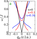
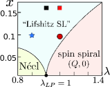
Figure 1: Panel (a): Theoretical HG dispersions for $\lambda=1.1$ and for two values of doping, $x=0$.1 (red) and $x=0$.16 (blue). The black line represents the magnon dispersion in the parent undoped compound ($x=0$). Panel (b): Zero temperature $\lambda-x$ phase diagram of extended $t-J$ model consists of three phases, Neel, Lifshitz spin liquid, Spin Spiral Kharkov2018a . The tricritical Lifshiz point is $\lambda=1$, $x=0$. The squares, the circle, and the star are the points considered in the text as examples.

Theoretical models of the magnetic dispersion and the $(\pi,\pi)$ resonance are split into two classes, models based on the normal Fermi liquid picture with a large Fermi surface and usual electrons with spin Abanov2002 ; Onufrieva2002 ; Sherman2003 ; Eremin2005 ; Eremin2012 , and models based on the picture of a doped Mott insulator with a small Fermi surface and spinless holons Milstein2008 ; James2012 . All early models have been motivated by experimentKeimer1995 in optimally doped YBa₂Cu₃O₇ and belong to the first class. In this approach the $(\pi,\pi)$ resonance is explained as a spin exciton in the d-wave SC phase. These models are consistent with observation (O2), but inconsistent with all other observations which appeared later and that indicate that SC is not essential. In light of this inconsistency the spin exciton model was modified by artificial introduction of localised spins in the normal Fermi liquid model Sherman2003 ; Eremin2012 . This modification partially explains the observation (O4) (in addition to (O2)), but is still inconsistent with all other observations.

The second theoretical approach based on the picture of a doped Mott insulator was developed later after the low doping data were obtained. This approach naturally explains the observation (O1). The model of Ref.Milstein2008 is based on the picture of static spin spiral Shraiman90 . This model explains the observations (O1),(O3),(O5), but fails in all other points. The model of Ref.James2012 explains (O1) and partially (O4), but fails in all other points. Thus, the theoretical situation is unsatisfactory.

In the present work we pursue the approach of a lightly doped Mott insulator. There are four major experimental facts supporting the Mott insulator approach, here they are.

(F1) According to NMR the nearest site antiferromagnetic exchange, $J\approx 125$meV, is doping independent Imai1993 .

(F2) The second fact is the observation (O1) from the HG list presented above. It is hardly possible to shrink the HG to zero at zero doping in any model but doped Mott insulator.

(F3) RIXS data indicate that the high energy magnons, $\omega\sim 200-300meV$, in doped compounds are practically the same as in undoped ones, this includes both the dispersion and the spectral weight LeTacon11 .

(F4) The momentum integrated structure factor $S(\omega)$ measured in neutron scattering at $\omega\approx 50-80$meV in doped compounds is practically the same as in undoped ones. We will demonstrate this observation at the end of this paper.

These four facts unambiguously favour the Mott insulator approach.

The Mott insulator approach necessarily implies a small Fermi surface, Fig.2a, and this immediately leads to two conclusions that are evident without calculations. The first conclusion concerns superconductivity. The Fermi energy is proportional to the doping x, $\epsilon_{F}\sim xJ$. For optimal doping, $x=0.15$, the Fermi energy is $\epsilon_{F}\approx 35$meV. On the other hand we know experimentally that the superconducting gap is $\Delta_{SC}\approx 30$meV. Thus, all cuprates are in the strong coupling limit, $\epsilon_{F}\approx\Delta_{SC}$. The second conclusion concerns the spin liquid ground state. Consistently with small Fermi surface the number of charge carriers measured via Hall effect is equal to the doping $x\ll 1$. The number of uncompensated spins in a doped Mott insulator is $1-x$, so unlike a normal metal the number of spins is much larger than the number of charge carriers. We also know that the static magnetic order disappears above several per cent doping, when $x\ll 1-x$. These points indicate that spin and charge are separated and that quantum spin fluctuations ’melt’ the static magnetic order to a spin liquid (SL). Of course the notion of SL in cuprates is not new, the same motivation is behind the RVB SL model Anderson .

The present work is based on the recent progress in understanding of the SL state of cuprates Kharkov2018a . The SL in cuprates is different to the RVB model. It is the quantum critical Ioffe-Larkin type SL (“Lifshitz SL”) Kharkov2018a . This insight allows us to perform calculations and to explain all properties of the HG. There are the following sections in the paper. II. Magnetic response in the spin liquid phase. III. Calculated q-scans of the spectral function at optimal doping. IV. Magnetic criticality mechanism of the hour-glass dispersion. V. Is there a hole in the hour-glass? VI. Calculated q-scans of the spectral function in the underdoped case. Emergent incommensurate magnetic order. VII Wine-glass dispersion. VIII. Lifshitz spin liquid fingerprint relation. IX. Conclusions. Technical details are presented in Appendices A,B,C.

II Magnetic response in the spin liquid phase

We start with the zero temperature $\lambda-x$ phase diagram from Ref. Kharkov2018a presented in Fig.1b. The dimensionless parameter $\lambda$ defined as

$$\lambda=\frac{2g^{2}m^{*}}{\pi\rho_{s}}$$ (1)

plays a crucial role in the theory, it controls magnetic criticality. Here $m^{*}$ is the holon effective mass, $\rho_{s}$ is bare spin stiffness, and $g$ is the holon-magnon coupling constant, for details see Appendix A. The Lifshitz quantum tricritical point is $\lambda=1$, $x=0$. Three phases meet at the tricritical point, the collinear Néel phase, Lifshitz SL, the spin spiral state, see Appendix B. The Lifshitz SL is characterised by a parameter $\Delta$ that we term the SL gap. It is worth noting that in the exact sense the SL is gapless. Below we also introduce and explain the spin pseudogap $\Delta_{s}$. Besides the Lifshitz quantum tricritical point there is another critical point, $\lambda=2$, related to the phase separation, see Appendix A. Our analysis is based on the extended $t-J$ model which is described by the antiferromagnetic exchange $J\approx 125$meV and hopping parameters. The relation between parameters of the extended $t-J$ model and $\lambda$ is discussed in Appendix A. Having the nearest site hopping parameter $t$ fixed, $t/J\approx 3$, one can vary distant hopping parameters. In principle this results in variation of $\lambda$ in a very broad range, $0<\lambda<\infty$. Using values of the hopping matrix elements obtained in LDA calculations andersen95 one can obtain the following range for the criticality parameter $\sim 0.7\leq\lambda\leq 2$, see Appendix A. Nevertheless this range of $\lambda$ is too wide, it is even sufficient to drive the system to the phase separation. Experiments indicate that most cuprates are magnetically disordered except of the emergent magnetism at very low doping. This observation allows us to restrict the range to approximately $\lambda=1.1\pm 0.3$ shown in Fig.1b. The criticality parameter $\lambda$ can vary from one cuprate family to another and can slightly depend on doping.

To avoid misunderstanding we note that the magnetic criticality we are talking about is unrelated to the quantum critical point at doping $x=x^{*}\approx 0.2$ (the endpoint of the “pseudogap” regime) where presumably the small Fermi surface is transformed to the large one Taillefer2010 . We only consider $x<x^{*}$ and claim that all hole doped cuprates are close to the Lifshitz magnetic criticality. One can also call it the “hidden” criticality. It is hidden in the sense that unlike doping, the parameter $\lambda$ cannot be directly measured.

The first message of our paper is that the HG dispersion is a direct consequence of the SL gap and the Lifshitz magnetic criticality. SC plays a secondary role, it only influences the particle-hole decay phase space and narrows the spectral lines in the lower part of HG. The first message resolves the generic problems (O1)-(O5) listed in the introduction. The second message is that due to proximity to the quantum critical point a small ($\sim 10\%$) variation of $\lambda$ results in sizeable change of the lower part of HG. This explains the point (O6) from the observation list.

We introduce superconductivity in the theory ad hoc via the phenomenological d-wave SC gap

$$\Delta_{\bm{k}}=\Delta_{SC}\frac{1}{2}(\cos k_{x}-\cos k_{y})\ .$$ (2)

For details see Appendix C. In our theory the $(\pi,\pi)$ resonance (the neck of the HG) is unrelated to SC. The resonance is a manifestation of the SL gap $\Delta$ which is practically the same in the N state and in the SC state. Quite often in neutron scattering papers the energy of the neck of HG is denoted by $E_{cross}$, this is the same as the SL gap, $\Delta=E_{cross}$. The gap $\Delta$ was calculated in Ref. Kharkov2018a and is plotted versus doping in Fig.2b.

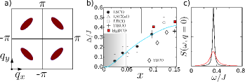
Figure 2: Panel (a): Small Fermi surface and momenta $q_{x}$, $q_{y}$ for magnetic scattering. Panel (b): The spin liquid gap versus doping (cyan line) Kharkov2018a . The theoretical curve corresponds to $\lambda=1$. Points show experimental data. In different compounds values of $\lambda$ can be somewhat different and this explains scattering of experimental points. Panel (c): The $\omega$-scan of the spectral function at $q=0$. The black solid line illustrates the perfect $\delta$-function, and the dashed red line shows the temperature (disorder) broadened line.

The scattering of experimental points in this plot is one of the manifestations of the observation (O6) which is explained by proximity to the magnetic criticality.

We describe magnetic response at energy $\omega\lesssim J$ in terms of fluctuating staggered magnetisation ${\vec{n}}$. The Green’s function of the $\vec{n}$-field in the SL phase reads, see Appendix A3,

$$D(\omega,\bm{q})=\ \frac{16J\sqrt{1-\mu x}}{\omega^{2}-c^{2}q^{2}-\Delta^{2}-\Pi(\omega,\bm{q})+i0}.$$ (3)

Here $\Delta$ is the SL gap and $\Pi(\omega,q)$ is the magnon polarisation operator. The magnon speed is $c\approx c_{0}\sqrt{1-\mu x}$, where $c_{0}\approx\sqrt{2}J$ is the magnon speed in the undoped compound. The coefficient $\mu\approx 4$ has been calculated numerically within the $t-J$ model Kharkov2018a . The uncertainty of this calculation is about $4<\mu<5$. The coefficient $\mu$ determines the dispersion slope softening at high energy. The softening is known experimentally and therefore the value of $\mu$ can be also extracted from experimental data. This gives the same uncertainty interval $4<\mu<5$.

The magnetic spectral function is $S(\omega,\bm{q})=-\frac{A}{16\pi J}{\mbox{I}m}D$. The proportionality coefficient $A$ depends on the on-site magnetic moment, Cu atomic form factor, etc. This coefficient is practically the same for all hole doped cuprates, at least for the single layer cuprates. The spectral function in the parent compound (Néel state, $x=0$) is

$$S_{Neel}(\omega,\bm{q})=A\delta(\omega^{2}-c_{0}^{2}q^{2}).$$ (4)

The holon polarisation operator $\Pi(\omega,\bm{q})$ calculated in Appendix C is a complex function of $\omega$ and $\bm{q}$, however $\Pi(\omega,0)=0$. Therefore, the spectral function at finite doping at $q=0$, $S(\omega,0)=A\sqrt{1-\mu x}\delta(\omega^{2}-\Delta^{2})$, is a perfect $(\pi,\pi)$-resonance shown in Fig.2c. Impurities and finite temperature give rise to a broadening illustrated by the red dashed line in Fig.2b. Importantly, the spectral weight is independent of the broadening and is defined by the SL gap $\Delta$ in the particular compound:

$$W=\int_{0}^{\infty}S(\omega,0)d\omega\approx\frac{A\sqrt{1-\mu x}}{2\Delta}\ .$$ (5)

III Calculated q-scans of the spectral function at optimal doping

In order to explain mechanism of the HG we consider separately the upper and the lower part of the HG, see Fig.1a. In a crude approximation one can neglect the polarisation operator in Eq.(3) for the upper part of the HG and this results in the dispersion

$$\omega_{q}\approx\sqrt{\Delta^{2}+c_{0}^{2}(1-\mu x)q^{2}}\ .$$ (6)

Of course we can do better than this crude approximation. In Fig.3 we plot $q_{x}$-scans of the spectral function calculated numerically (for definition of axes see Fig.2a). The calculation accounts for the polarisation operator and is performed for $x=0.16$ and six values of $\omega$.

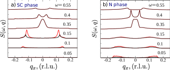
Figure 3: Calculated momentum scans of the spectral function for $x=0.16$, $\Delta=0.35J$, $\Delta_{SC}=0.2J$ and six different energies. Energies in units of $J$ are shown near the respective lines. Panel (a) corresponds to the SC-state and panel (b) to the N-state. Black curves correspond to $\lambda=1$ and red curves correspond to $\lambda=1.1$. Black and red practically coincide for higher energies.

The value of the SL gap is taken from Fig.2b, $\Delta=0.35J$, and $\Delta_{SC}=0.2J\approx 25$meV, see Appendix C. Panel (a) in Fig. 3 corresponds to the SC state and panel (b) to the N state com3 . The plot demonstrates that the upper part of the HG, $\omega>\Delta$, is only weakly sensitive to SC in agreement with observation (O4). In both SC and N phases the polarisation operator gives a broadening and some asymmetry of peaks in the spectral function, but overall the upper part of HG is consistent with crude Eq.(6). On the other hand according to Fig.3 sharp peaks in the lower part of HG, $\omega<\Delta$, exist in the SC state and disappear in the N state in agreement with observation (O2). However, the peaks are still present in the N-state, they just become very broad due to the decay to the particle-hole continuum. The spectra in Fig.3a correspond to the HG dispersion plotted in Fig.1a by the blue line. We plot the dispersion again in Fig.4a with indication of SL gap $\Delta$ and the spin pseudogap $\Delta_{s}$.

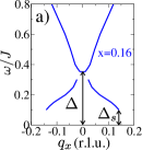
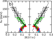
Figure 4: Panel a: The HG dispersion for x=0.16 deduced from spectra in Fig.3a. In this plot we indicate the SL gap $\Delta$ and the spin pseudogap $\Delta_{s}$. Panel b: The HG dispersion in La_1.84Sr_0.16CuO₄ from Ref. Vignolle07

According to Fig.3a in the SC state the magnetic response is strongly suppressed at low frequencies, $\omega\lesssim 0.1J$. The suppression can be described by the spin pseudogap $\Delta_{s}$ indicated in Fig.4a. Unlike the true gap $\Delta$, the $\Delta_{s}$ is a pseudogap since at the incommensurate q-points there is some response down to zero energy. In the N state, Fig.3b, the low energy response is strongly enhanced. The presence of the zero-frequency magnetic response in the vicinity of the incommensurate wave vector $Q\approx 0.14$r.l.u. results in a nonzero NMR relaxation rate. We illustrate sensitivity of the spin pseudogap $\Delta_{s}$ to the magnetic criticality parameter $\lambda$ by plotting in Fig.3 the spectral function for two values of $\lambda$: $\lambda=1$ (black) and $\lambda=1.1$ (red). These values correspond to red and black squares on the phase diagram Fig.1b. Both in the SC and the N states the upper part of HG is not sensitive to the small variation of $\lambda$. Conversely, the lower part in the SC state, $\omega<\Delta$, is very sensitive. Naturally the spin pseudogap $\Delta_{s}$ is smaller at $\lambda=1.1$ compared to that at $\lambda=1$, since the former is closer to the phase boundary in Fig.1b.

Two dimensional ($q_{x},q_{y}$) colour maps of the calculated structure factor corresponding to the “red” spectra in Fig.3a are presented in Fig.5. The maps are close to data for La_1.84Sr_0.16CuO₄, Fig. 1 in Ref. Vignolle07 .

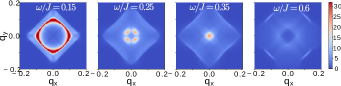
Figure 5: Colour maps of fixed energy $(q_{x},q_{y})$-scans of magnetic spectral function $S(\omega,q)$ for $x=0.16$ in SC phase. The magnetic criticality parameter $\lambda=1.1$, the SL gap is $\Delta=0.35J$, the SC gap is $\Delta_{SC}=0.2J$.

Detail comparison shows that La_1.84Sr_0.16CuO₄ is slightly more critical. Increasing $\lambda=1.1$ to $\lambda\approx 1.15-1.2$ we can even better reproduce data of Ref. Vignolle07 However, we do not perform the fit due to the reason explained in the Section VIII.

IV Magnetic criticality mechanism of the hour glass dispersion

The results presented in the previous section indicate that the HG is driven by the SL Lifshitz magnetic criticality, SC plays a secondary role and leads to the spectral line narrowing in the lower part of HG. In order to elucidate this point we plot in Fig.6 denominators of the Green’s function (3) versus $q_{x}$ for $x=0.16$. At $\omega=0$ the denominator is real and Fig.6a displays the $\omega=0$ denominator in the SC state for three different values of $\lambda$. For $\lambda=1.1$ and $\lambda=1.25$ the denominator is negative indicating stability of the SL phase. However, at $\lambda=1.36$ the denominator vanishes, $D^{-1}=0$, at $q_{x}\approx 0.135$ r.l.u. indicating condensation of the spin spiral with this wave vector, see the phase diagram Fig.1b. In Fig.6b we plot the denominator in the SC state for $\omega=0.15J$ and $\lambda=1.1$,

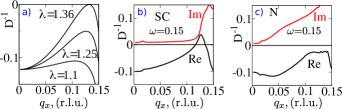
Figure 6: Denominators of the Green’s function (3) versus $q_{x}$ for $x=0.16$, $\Delta=0.35J$, $\Delta_{SC}=0.2J$. Panel (a): SC state, $\omega=0$, three different values of $\lambda$. Panel (b): SC state, $\omega=0.15J$, $\lambda=1.1$, real (black) and imaginary (red) parts. Panel (c): N state, $\omega=0.15J$, $\lambda=1.1$, real (black) and imaginary (red) parts.

and in Fig.6c we plot the same denominator but in the N state. In the SC state the Green’s function denominator is close to zero at $q_{x}\approx 0.12$ r.l.u. and this results in a narrow peak in the $\omega=0.15J$ red curve in Fig.3a. In the N state the real part of the denominator is also small, but the imaginary part is large, thus the magnetic critical enhancement just results in a very broad structure in the $\omega=0.15J$ red curve in Fig.3b.

Thus the HG is a collective excitation driven by the Lifshitz magnetic criticality. The role of SC is just to suppress the decay rate of the collective excitation.

V Is there a hole in the hour glass?

Sometimes experimental HG dispersion is plotted with a hollow “neck” as it is shown in Fig.4b. We think that the hollow neck does not exist, but we understand how it can mistakenly arise in the analysis of experimental data. Fig.3a demonstrates pairs of narrow peaks for scans above and below the HG neck and a broad peak at the neck $\omega=\Delta=0.35J$. An assumption that the broad peak consists of two narrow peaks leads to the hollow neck. However, we believe this is wrong, the neck of the HG is intrinsically broad. There is no hole in HG.

VI Calculated q-scans of the spectral function in the underdoped case. Emergent incommensurate magnetic order

Next we look at the lower doping, $x=0.1$. The SL gap according to Fig.2b is $\Delta=0.3J$. We keep the value of the magnetic criticality parameter unchanged, $\lambda=1.1$, but the value of the SC gap is reduced, $\Delta_{SC}=0.1J\approx 13$meV, see Appendix C. Fig.7 presents calculated $q_{x}$-scans of the spectral function for six values of $\omega$.

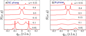
Figure 7: Calculated momentum scans of the spectral function for $x=0.1$, $\Delta=0.3J$, $\Delta_{SC}=0.1J$, $\lambda=1.1$, and six different energies. Energies in units of $J$ are shown near the respective lines. Panel (a) corresponds to the SC-state and panel (b) to the N-state.

The red circle on the phase diagram Fig.1b corresponding to these parameters is located close to the critical line. Therefore, the low frequency response in Fig.7 is strongly enhanced compared to that in Fig.3. In this case the spin pseudogap is practically zero, $\Delta_{s}\approx 0$. Moreover, the lower part of HG becomes evident even in the N state in agreement with the observation (O3). Further decreasing of doping would result in an emergent static incommensurate magnetic order in agreement with the observation (O5).

The HG dispersion deduced from Fig.3a and Fig.7a, are plotted in Fig.1a by the blue and red lines, respectively.

VII Wine Glass dispersion

It is clear from the above discussion that decreasing of the magnetic criticality parameter $\lambda$ reduces the intensity of the lower part of the HG. In Fig.8 we present momentum scans for $\lambda=0.9$. All other parameters are the same as that in Fig.7, $x=0.1$, $\Delta=0.3J$, $\Delta_{SC}=0.1J$. The blue star on the phase diagram Fig.1b corresponds to this set of parameters.

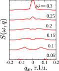
Figure 8: Calculated momentum scans of the spectral function in the SC state for $x=0.1$, $\Delta=0.3J$, $\lambda=0.9$, and 6 different energies. Energies in units of J are shown near the respective lines.

In Fig. 8 the intensity in the lower part of the spectrum is dramatically reduced compared to that in Fig.7. At the same time the upper part of the spectrum is practically the same. Thus, reducing $\lambda$ one drives the HG dispersion to the “wine-glass” regime reported in Refs. Chan2016 ; Chan16a

VIII Lifshitz spin liquid fingerprint relation

In the previous sections we have explained all the major HG observations (O1)-(O6) listed in the introduction. Is there a further experimental confirmation of the developed theory? The answer is yes. The central point of the theory is that the Lifshitz SL is very similar to the parent antiferromagnet. Most explicitly this point is reflected in Eqs.(4),(5). The spectral weight W in the SL phase, Eq.(5), is expressed via the coefficient A known from the parent antiferromagnet, Eq.(4). For this reason we call Eq.(5) the Lifshitz SL “fingerprint” relation. Let us compare this relation with experimental data.

Using Eq.(4) and fitting the 5K data in Fig.4a of Ref. Matsuura2017 for undoped La₂CuO₄ we find $A\approx 0.35\mu_{B}^{2}eV/f.u.$ Hence, using Eq.(5) we plot in Fig.9a theoretical curves for the product $W\times\Delta$ versus doping. We know the value of the coefficient $\mu$ in (5) only approximately, therefore we present curves for $\mu=4,5$ to indicate theoretical uncertainty. At the same Fig.9a we present experimental points extracted from data for La_2-xSr_xCuO₄ (red) Matsuura2017 and HgBa₂CuO_4+δ (blue) Chan2016 ; Chan16a . The red point at $x=0$ gives the normalisation of the theoretical curve. The agreement is quite good, the data are consistent with the SL “fingerprint” relation.

It would be very interesting to perform a similar analysis for YBCO. The compound has theoretical complications related to the double layer structure and to the oxygen chains, but these issues are probably resolvable. The major problem is that there is not enough data with absolute normalisation of intensity.

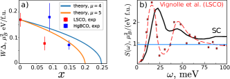
Figure 9: Panel (a): The SL sum rule $W\Delta=0.5A\sqrt{1-\mu x}$, Eq.(5), versus doping. Two theoretical curves indicate uncertainty of $\mu$. The red points are extracted from La_2-xSr_xCuO₄ data Matsuura2017 and the blue points from HgBa₂CuO_4+δ data Chan2016 ; Chan16a . Panel (b): Black line represents theoretical $q$-integrated spectral function $S(\omega)$ for $x=0.16$, $\Delta=0.35J$, $\Delta_{SC}=0.2J$, $\lambda=1.1$. The red line is experimental $S(\omega)$ for La_1.84Sr_0.16CuO₄, Ref. Vignolle07 The blue horizontal line shows $S(\omega)$ in La₂CuO₄.

The next point we address is the $q$-integrated spectral function $S(\omega)=\int S(\omega,{\bm{q}})\frac{d^{2}q}{(2\pi)^{2}}$. To be specific we take the same set of parameters as that in Fig.3, $x=0.16$, $\Delta=0.35J$, $\lambda=1.1$, $\Delta_{SC}=0.2J$. The calculated spectral function in the SC state is shown in Fig.9b by the black line. For normalisation we use the value of $A$ extracted from undoped La₂CuO₄ as described in the second paragraph of this section. In the same Fig.9b we plot the experimental curve (red) for La_1.84Sr_0.16CuO₄, Ref.Vignolle07 The agreement between the theory and the experiment both in shape and in the absolute normalisation is good. The characteristic double hump structure has been also observed in YBa₂Cu₃O_6.5, Ref.Keimer1997a As we pointed out above, a slight increase of criticality parameter, $\lambda=1.1\to\lambda\approx 1.15-1.2$ would shift the low peak down close to the experimental position. In principle one can try to fit the data by changing $\lambda$. However, there are recent evidences wagman2015 ; Xu2014 indicating a phonon with energy $\omega\approx 18-20$meV. The phonon adds some intensity to the lower peak in Fig. 9b. Of course the phonon is not described by our theory. This is why we do not fit data of Ref.Vignolle07 presented in Fig. 9b.

According to Eq.(4) the $q$-integrated spectral function in the parent antiferromagnet is $S(\omega)=\frac{A}{8\pi J^{2}}\approx 0.95\mu_{B}^{2}/(eV\ f.u.)$. This value is shown in Fig.9b by the blue horizontal line. In the energy interval above the neck of HG, $\omega=50-80$meV, this value coincides with $S(\omega)$ for La_1.84Sr_0.16CuO₄ presented in the same figure. This proves the point (F4) listed in the Introduction. The same point is true for YBCO. Relevant data are presented in Fig.2a of Ref.Keimer1997a Solid lines in this figure represent $S(\omega)$ in YBa₂Cu₃O_6.5 for three different temperature and the horizontal dashed line shows $S(\omega)$ in the parent antiferromagnet Bourges2019 . From these data we conclude that in the interval $\omega=50-80$meV the structure factor $S(\omega)$ in YBa₂Cu₃O_6.5 and in the parent antiferromagnet has the same value.

IX Conclusions

We show that the hour-glass magnetic dispersion in underdoped cuprates is driven by properties of the Lifshitz magnetic critical spin liquid. Superconductivity plays a secondary role and only responsible for the narrowing of the spectral lines. We list the six major observations related to the hour-glass dispersion and explain all of them. We propose a spin liquid “fingerprint relation” and demonstrate that neutron scattering data support the relation.

Appendix A Effective action

A.1 Extended $t-J$ model

The Hamiltonian of the extended $t-J$ model reads Anderson87 ; Emery87 ; Zhang88

$$H=-t\sum_{\langle ij\rangle}c^{\dagger}_{i,\sigma}c_{j,\sigma}-t^{\prime}\sum_{\langle\langle ij\rangle\rangle}c^{\dagger}_{i,\sigma}c_{j,\sigma}-$$

$$t^{\prime\prime}\sum_{\langle\langle\langle ij\rangle\rangle\rangle}c^{\dagger}_{i,\sigma}c_{j,\sigma}+J\sum_{\langle i,j\rangle}\left[\bm{S}_{i}\cdot\bm{S}_{j}-\frac{1}{4}N_{i}N_{j}\right],$$ (7)

where $c^{\dagger}_{i\sigma}$ ($c_{i\sigma}$) is the creation (annihilation) operator for an electron with spin $\sigma=\uparrow,\downarrow$ at Cu site $i$; the operator of electron spin reads $\bm{S}_{i}=\frac{1}{2}c^{\dagger}_{i\alpha}\bm{\sigma}_{\alpha\beta}c_{i\beta}$. The electron number density operator is $N_{i}=\sum_{\sigma}c^{\dagger}_{i\sigma}c_{i\sigma}$, where $x$ is the hole doping, so that the sum rule $\langle N_{i}\rangle=1-x$ is obeyed. In addition to Hamiltonian (A.1) there is the no double occupancy constraint, which accounts for a strong electron-electron on-site repulsion. The value of superexchange is approximately the same for all cuprates, $J\approx 125$meV. The superexchange has been directly measured and shown to be independent of doping Imai1993 . While in Eq.(A.1) we present only three hopping matrix elements, the nearest site hopping $t$, the next nearest site hopping $t^{\prime}$, and the next next nearest site hopping $t^{\prime\prime}$, we know from LDA calculations andersen95 that more distant hoppings, $t^{(3)}$, $t^{(4)}$ and even $t^{(5)}$ are also significant. Unfortunately values of the hopping matrix elements cannot be directly measured. It is widely believed that the value $t\approx 400meV\approx 3J$ is reliable and common for all cuprates, we use this value in the present work. However, values of the distant hopping matrix elements are rather uncertain and can vary from one family to another.

The Fermi surface of a lightly doped extended $t-J$ model consists of Fermi pockets shown in Fig.2a and centred at the nodal points $\mathbf{k}_{0}=(\pm\pi/2,\pm\pi/2)$, and $\mathbf{k}_{0}=(\pm\pi/2,\mp\pi/2)$. The single hole dispersion can be parameterised as Sushkov1997

$$\epsilon_{\bm{k}}=\beta_{1}(\gamma_{\bm{k}}^{+})^{2}+\beta_{2}(\gamma_{\bm{k}}^{-})^{2},\ \ \gamma_{\bm{k}}^{\pm}=\frac{1}{2}(\cos k_{x}\pm\cos k_{y}),$$

$$\epsilon_{\bm{k}}\approx\beta_{1}\frac{p_{1}^{2}}{2}+\beta_{2}\frac{p_{2}^{2}}{2}.$$ (8)

Here ${\bf p}={\bf k}-\mathbf{k}_{0}$, see Fig.2a. We set the lattice spacing equal to unity, $a=3.81\AA\rightarrow 1$. The second line in Eq.(A.1) corresponds to the quadratic expansion of the fermion dispersion in the vicinity of the centers of Fermi pockets. The ellipticity of the holon pocket is $\sqrt{\beta_{1}/\beta_{2}}$. The Fermi energy is related to doping as

$$\epsilon_{F}\approx\pi\beta x,$$

$$\beta=\sqrt{\beta_{1}\beta_{2}}=\frac{1}{m^{*}}.$$ (9)

Values of the inverse effective masses $\beta_{1}$, $\beta_{2}$ follow from Hamiltonian (A.1). They have been calculated using self-consistent Born approximation (SCBA), see Refs.Sushkov1997 ; Sushkov04 The values strongly depend on distant hopping parameters which are essentially unknown, even $t^{(3)}-t^{(5)}$ significantly influence SCBA results. For illustration we present here values of $\beta_{1}$, $\beta_{2}$ obtained for several sets of the distant hopping parameters. We consider only the sets that result in positive $\beta_{1}$ and $\beta_{2}$. For the “pure” $t-J$ model, $t^{\prime}=t^{\prime\prime}=t^{(3)}=t^{(4)}=t^{(5)}=0$, the values are $\beta_{1}=1.96J$, $\beta_{2}=0.30J$. For the set $t^{\prime}\approx 0.23J$, $t^{\prime\prime}=0$, $t^{(3)}=t^{(4)}=t^{(5)}=0$ one gets the Van Hove singularity, $\beta_{2}=0$. On the other hand in the limit $t^{\prime\prime}\gg t^{\prime},J$ the inverse masses are very large $\beta_{1}\approx\beta_{2}\approx 8t^{\prime\prime}\gg J$. For the middle of the LDA range, Ref.andersen95 , $t^{\prime}=-0.5J$, $t^{\prime\prime}=0.5J$, $t^{(3)}=t^{(4)}=t^{(5)}=0$ the inverse masses are $\beta_{1}\approx 2.76J$, $\beta_{2}\approx 2.62J$. While we can claim that $\beta=\sqrt{\beta_{1}\beta_{2}}\sim 2$, the so strong dependence on unknown parameters indicates that in the end the effective masses and especially the ellipticity of the Fermi pocket have to be taken from experiment.

Even more important than the effective masses is the dimensionless magnetic criticality parameter Sushkov04 ; Milstein2008

$$\lambda=\frac{8g^{2}}{\pi\sqrt{\beta_{1}\beta_{2}}}.$$ (10)

Here $g=Zt$ is the magnon-holon coupling constant, $Z$ is the holon quasiparticle residue. In theory by varying $t^{\prime}$ and $t^{\prime\prime}$ one can vary $\lambda$ from zero to infinity. In the large $t^{\prime\prime}$ limit, $t^{\prime\prime}\gg t^{\prime},J$, the parameter is very small, $\lambda\to 0$. On the other hand near the Van Hove singularity, $\beta_{2}\to 0$, the parameter is very large $\lambda\to\infty$. For the “pure” $t-J$ model, $t^{\prime}=t^{\prime\prime}=t^{(3)}=t^{(4)}=t^{(5)}=0$ the criticality parameter value is $\lambda=2.51$. For the middle of the LDA range andersen95 , $t^{\prime}=-0.5J$, $t^{\prime\prime}=0.5J$, $t^{(3)}=t^{(4)}=t^{(5)}=0$, the criticality parameter value is $\lambda=1.1$. Within the overall LDA range of the hopping parameters andersen95 $\lambda$ varies from 1 to 2. Numerically the difference between $\lambda=2$ and $\lambda=1$ is not that large, but physically the difference is enormous. The value $\lambda\geq 2$ implies that the system is unstable with respect to the phase separation, see Ref. Chubukov95 and Ref.Sushkov04 So, the “pure” $t-J$ model with $\lambda\approx 2.5$ is unstable and hence inconsistent with experiment. On the other hand the value $\lambda=1$ corresponds to the stable spin liquid phase which is perfectly consistent with experiment, see Fig.1b and Ref. Kharkov2018a While from LDA+SCBA we can claim that $\lambda\sim 1$, the strong dependence on unknown parameters indicates that in the end the value of $\lambda$ must be taken from experiment. Based on the phase diagram Fig.1b we see that values $0.8<\lambda<1.3$ are generally consistent with data.

To summarise this section: we base our analysis on the extended $t-J$ model and use the value $J\approx 125$ meV known from experiment. In the calculation we use the value $t=3J$, we have checked that a variation of t within $2.5J<t<3.5J$ influences our results very weakly. However, a variation of distant hopping matrix elements, $t^{\prime}$, $t^{\prime\prime}$, $t^{(3)}$,… has an enormous effect on physics. Variation of these matrix elements within the window given by LDA calculations andersen95 can drive the system from the Neel state through the spin liquid state to the spin spiral state and even to the phase separation. Based on the spin liquid theory we conclude that the range $0.8<\lambda<1.3$ is consistent with experimental observations, so in our calculations we use this range. Specifically in the paper we present results for $\lambda=1.1$, $\lambda=1$, and $\lambda=0.9$ to demonstrate sensitivity to the criticality parameter. The value of the effective mass is less important, in the paper we present results for $\beta=\sqrt{\beta_{1}\beta_{2}}=2J$ ($m^{*}=2.1m_{e}$) and $\beta_{1}/\beta_{2}=6$. We have checked that the set $\beta=\sqrt{\beta_{1}\beta_{2}}=3J$ and $\beta_{1}/\beta_{2}=4$ results in practically the same answers.

A.2 Quantum field theory: the low energy limit of the extended $t-J$ model

While the $t-J$ model is the low energy reduction of the three band Hubbard model, the total energy range in the $t-J$ model, $\Delta\epsilon\sim 8t\sim 24J\approx 3$eV, is still very large. Account for quantum fluctuations at lower energy scales practically unavoidably requires a quantum field theory approach. Theoretical arguments explaining this point have been discussed in several theoretical papers including our recent work Kharkov2018a . Here we repeat only experimental arguments supporting this statement. In Fig.10 we present magnetic dispersion along the $(1,0)$ direction taken from Ref. LeTacon11 The dispersion is based on combined data on resonant inelastic X-ray scattering and inelastic neutron scattering.

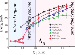
Figure 10: Magnetic dispersion along the $(1,0)$ direction. Points show combined data on resonant inelastic X-ray scattering and inelastic neutron scattering in NdBCO and YBCO at $T=15$K, Ref. LeTacon11 Vertical lines separate three different regimes that we call “infrared regime”, “intermediate regime”, and “ultraviolet regime”.

The data indicate three distinct regimes separated in Fig.10 by vertical lines. In the “ultraviolet regime” the dispersion only very weakly depends on doping, practically independent. This is where our “fact” (F2) in the Introductions comes from. In the “intermediate regime” there is a significant softening with doping and the most dramatic doping dependence takes place in the “infrared regime”. The low energy effective field theory is relevant to the “infrared” and the “intermediate” regimes. In these regimes energies of magnetic excitations and energies of holons are small, $\omega,\epsilon<2J$. On the other hand in the “ultraviolet regime” the energies are large, $\omega\sim 2J$ and $8t>\epsilon\gtrsim 2J$. The field theory has the ultraviolet cutoff $\Lambda_{q}$ which is the upper edge of the “intermediate regime” as it is indicated in Fig.10. The value of the cutoff that follows from the data is $\Lambda_{q}\sim 0.2$r.l.u). The same value follows from the theory, see Ref. Kharkov2018a

The low energy Lagrangian of the $t-J$ model was first derived in Ref.Shraiman90 with some important terms missing. The full effective Lagrangian was derived in Ref.Milstein2008 This approach necessarily requires an introduction of two checkerboard sublattices, independent of whether there is a long range AFM order or the order does not exist. The two checkerboard sublattices allow us to avoid a double counting of quantum states in the case when spin and charge are separated. A holon carries charge and does not carry spin, but it can be located at one of the sublattices and this is described by the pseudospin $1/2$. Due to the checkerboard sublattices the Brillouin zone coincides with magnetic Brillouin zone (MBZ) even in the absence of a long range AFM order. Therefore, there are four half-pockets in Fig.2a or two full pockets within MBZ. Finally, the Lagrangian readsMilstein2008

$${\cal L} = \frac{\chi_{\perp}}{2}{\dot{\vec{n}}}^{2}-\frac{\rho_{s}}{2}\left({\bm{\nabla}}{\vec{n}}\right)^{2}$$

$$+ \sum_{\alpha}\left\{\frac{i}{2}\left[\psi^{{\dagger}}_{\alpha}{{\cal D}_{t}\psi}_{\alpha}-{({\cal D}_{t}\psi_{\alpha})}^{{\dagger}}\psi_{\alpha}\right]-\psi^{{\dagger}}_{\alpha}\epsilon_{\alpha}({\bf\cal P})\psi_{\alpha}\right.$$

$$+ \left.\sqrt{2}g(\psi^{{\dagger}}_{\alpha}{\vec{\sigma}}\psi_{\alpha})\cdot\left[{\vec{n}}\times({\bm{e}}_{\alpha}\cdot{\bm{\nabla}}){\vec{n}}\right]\right\}\ .$$

Fermions (holons) are described by a spinor $\psi_{\alpha}$ with the pseudospin $1/2$, and the vector of staggered magnetization ${\bm{n}}$ normalised as $\bm{n}^{2}=1$ corresponds to localised spins at Cu sites. The first line in (A.2) is $O(3)$ nonlinear sigma model that describes spin dynamics, the second line is the Lagrangian for non-interacting holons. The long covariant derivatives in Eq. (A.2) are defined as

$$\mathcal{\bm{P}}=-i\bm{\nabla}+\frac{1}{2}\vec{\sigma}\cdot[\vec{n}\times\bm{\nabla}\vec{n}],$$

$$\mathcal{D}_{t}=\partial_{t}+\frac{1}{2}\vec{\sigma}\cdot[\vec{n}\times\partial_{t}\vec{n}].$$

The index $\alpha=1,2$ enumerates two full holon pockets in Fig.2a. The term in the bottom line in Eq. (A.2) describes the coupling between holons and the staggered magnetisation. Pauli matrices $\bm{\sigma}$ in Eq. (A.2) act on the holon’s pseudospin and $\bm{e}_{\alpha}=1/\sqrt{2}(1,\pm 1)$ denotes a unit vector orthogonal to the face of the MBZ where the holon is located. The coupling constant $g$ enters Eq.(10).

The Lagrangian (A.2) is fully equivalent to the $t-J$ model Hamiltonian (A.1). In essence Eq. (A.2) originates from the Hamiltonian (A.1) rewritten in notations convenient for analysis of the low energy physics. The relation between (A.2) and (A.1) is the same as that between the nonlinear $\sigma$-model and the Heisenberg antiferromagnetic model on square lattice. The Lagrangian (A.2) contains five parameters, $\chi_{\perp}$, $\rho_{s}$, $\beta_{1}$, $\beta_{2}$, and $g$. Of course they can be expressed in terms of parameters of the “parent” $t-J$ model. We have already discussed $\beta_{1}$ and $\beta_{2}$. The coupling $g=Zt$ is related to $\lambda$, see Eq.(10), so it is also already discussed. In the limit $x\to 0$ the $\sigma$-model parameters $\chi_{\perp}$ and $\rho_{s}$ coincide with that of the 2D Heisenberg model on the square lattice, $\chi_{\perp}=1/8J$, $\rho_{s}=J/4$, up to an overall scalar prefactor in Lagranian (A.2) due to the renormalization of the spin magnitude by quantum fluctuations. The magnon speed is

$$c_{0}=\sqrt{\rho_{s}/\chi_{\perp}}=\sqrt{2}J.$$ (12)

A.3 Dependence of the Lagrangian parameters on doping

The small parameter of our theory is doping, $x\ll 1$. The Lagrangian parameters in subsection A2 are written in the limit $x\to 0$. Here we discuss the $x$-dependence of the parameters up to the linear in $x$ approximation. The first effect is renormalization of the $\sigma$-model parameters due to fermionic fluctuations at the high energy scale, $E\sim 8t\sim 24J$, see Ref. Kharkov2018a

$$\chi_{\perp}=\frac{1}{8J}\to\frac{1}{8J}$$

$$\rho_{s}=\frac{J}{4}\to\frac{J}{4}(1-\mu x)$$

$$c=\sqrt{\frac{\rho_{s}}{\chi_{\perp}}}\to c_{0}\sqrt{1-\mu x}$$ (13)

Note that the numerical coefficient $\mu\approx 4$ in the doping dependent prefactor is known only approximately, see Ref.Kharkov2018a

The magnon Green’s function generated by (A.2) above the spin liquid energy scale $\Delta$, $\Delta<\omega\lesssim J$ after taking into account Eqs.(A.3) reads

$$D(\omega,{\bm{q}})\propto\frac{\chi_{\perp}^{-1}}{\omega^{2}-c_{0}^{2}(1-\mu x)\bm{q}^{2}+i0}\ .$$ (14)

Hence the sum rule for the spin structure factor is

$$\int S(\omega,{\bm{q}})d\omega d^{2}q\propto\int ImD(\omega,{\bm{q}})d\omega d^{2}q\propto\frac{\Lambda_{q}}{\sqrt{1-\mu x}}$$ (15)

The integration is performed in limits $0<\omega<\infty$, $0<q<\Lambda_{q}$, where $\Lambda_{q}\approx 1.2\approx 2\pi*0.2(r.l.u.)$ (we remind that we set the lattice spacing equal to unity) is the ultraviolet cutoff of the theory. Eq.(15) implies that the spin sum rule is increasing with doping. Obviously the sum rule should be a doping independent constant. This implies that magnetic fluctuations at the scale $\omega\sim J\gg\Delta$ must generate the magnon quasiparticle residue

$$Z_{x}=\sqrt{1-\mu x}\ .$$ (16)

Eqs.(14),(15) must be multiplied by the residue and this makes the sum rule doping independent.

Appendix B The frustration mechanism behind the Lifshitz spin liquid

Here we explain the mechanism of the Lifshitz SL without going to technical details. The details are presented in Ref.Kharkov2018a The easiest way to understand how the Lifshitz SL arises due to frustration of spins by mobile holons is to stay in the Néel phase, $\lambda<1$, and to increase $\lambda$, see the phase diagram Fig.1b. In the Néel phase there is a collinear long range order $\langle n_{z}\rangle\neq 0$, and there is a quantum fluctuation $\langle n_{\perp}^{2}\rangle=\langle n_{x}^{2}\rangle+\langle n_{y}^{2}\rangle$. A calculation at small doping x gives the following answer for the fluctuation

$$\langle\vec{n}_{\perp}^{2}\rangle=\frac{x\beta}{2\rho_{s}}\ln\left(\frac{1}{1-\lambda}\right)+const\ .$$ (17)

When $\lambda$ is sufficiently close to unity the fluctuation is very large and this results in the quantum melting of the long range Néel order. This explains the Néel - Lifshitz SL transition line in Fig.1b. Similar arguments lead the Lifshitz SL - Spin Spiral transition line on the phase diagram, see Ref. Kharkov2018a

Appendix C Effect of superconductivity

With account of $Z_{x}$ the magnetic Green’s function in the SL phase reads Kharkov2018a

$$D(\omega,\bm{q}) = -i\int d^{2}rdte^{i\omega t+iqr}\langle T\left\{\bm{n}_{i}(\bm{r},t)\cdot\bm{n}_{i}(0,0)\right\}\rangle$$ (18)

$$= \frac{2}{\chi_{\perp}}\ \frac{Z_{x}}{\omega^{2}-c^{2}q^{2}-\Delta^{2}-\Pi(\omega,\bm{q})+i0}$$

Here $\Delta$ is the SL gap and $\Pi(\omega,q)$ is the magnon polarisation operator (fermionic loop). The magnon-holon interaction is given by the Lagrangian (A.2). Hence, a calculation of the magnon polarisation operator is relatively straightforward. In the calculation one can disregard superconducting pairing of holons or alternatively take the pairing into account. Results without the pairing we call the “normal state results”.

In the present work we introduce superconductivity in the theory ad hoc via the phenomenological d-wave SC gap. We use the simplest parametrization for the gap

$$\Delta_{\bm{k}}=\Delta_{SC}\gamma_{\bm{k}}^{-}\ .$$ (19)

In our numerical calculations we used the following values of the SC gap

$$x=0.16:\ \ \ \Delta_{SC}=0.2J$$

$$x=0.10:\ \ \ \Delta_{SC}=0.1J$$ (20)

Expressed in terms of parameters of the Lagrangian (A.2) the zero temperature polarisation operator in the SC phase reads sushkov1996

$$\Pi(\omega,q)=\frac{2\pi\lambda c^{2}}{m^{*}}\sum_{\alpha=1,2}q_{\alpha}^{2}\int\frac{d^{2}k}{(2\pi)^{2}}\left\{v^{2}_{\bm{k}}u^{2}_{\bm{k+q}}\right.$$ (21)

$$\left.+u_{\bm{k}}v_{\bm{k}}u_{\bm{k+q}}v_{\bm{k+q}}\right\}\left[\frac{1}{\omega-E_{\bm{k}}-E_{\bm{k+q}}+i0}+(\omega\to-\omega)\right],$$

where $q_{\alpha}={\bm{q}}\cdot{\bm{e}}_{\alpha}$ and $u_{\bm{k}}$ and $v_{\bm{k}}$ are Bogoliubov parameters:

$$u_{\bm{k}}=\sqrt{\frac{1}{2}\left(1+\frac{\xi_{\bm{k}}}{E_{\bm{k}}}\right)}$$

$$v_{\bm{k}}=sign(\gamma_{\bm{k}}^{-})\sqrt{\frac{1}{2}\left(1-\frac{\xi_{\bm{k}}}{E_{\bm{k}}}\right)}.$$ (22)

The quasiparticle dispersion reads

$$E_{\bm{k}}=\sqrt{\Delta_{\bm{k}}^{2}+\xi_{\bm{k}}^{2}},\quad\xi_{\bm{k}}=\epsilon_{\bm{k}}-\mu,$$ (23)

where the chemical potential $\mu$ is defined by the condition

$$x=2\sum_{\alpha=1,2}\int\frac{d^{2}k}{(2\pi)^{2}}v^{2}_{\bm{k}}\ .$$ (24)

Numerical evaluation of the polarization operator (21) is straightforward and we use it in the present work.

References

- (1) M. Arai, T. Nishijima, Y. Endoh, T. Egami, S. Tajima, K. Tomimoto, Y. Shiohara, M. Takahashi, A. Garrett, and S. M. Bennington, Phys. Rev. Lett. 83, 608 (1999).
- (2) P. Bourges, Y. Sidis, H. F. Fong, L. P. Regnault, J. Bossy, A. Ivanov, B. Keimer, Science 288, 1234 (2000).
- (3) S. M. Hayden, H. A. Mook, P. Dai, T. G. Perring, and F. Dogan, Nature 429, 531 (2004).
- (4) J. M. Tranquada, H. Woo, T. G. Perring, H. Goka, G. D. Gu, G. Xu, M. Fujita, and K. Yamada, Nature 429, 534 (2004).
- (5) V. Hinkov, P. Bourges, S. Pailhes, Y. Sidis, A. Ivanov, C. D. Frost, T. G. Perring, C. T. Lin, D. P. Chen, and B. Keimer, Nat. Phys. 3, 780 (2007).
- (6) M. Fujita, H. Hiraka, M. Matsuda, M. Matsuura, J. M. Tranquada, S. Wakimoto, G. Xu, and K. Yamada, J. Phys. Soc. Jpn. 81, 011007 (2012).
- (7) M. Vojta, T. Vojta, and R. K. Kaul, Phys. Rev. Lett., 97, 097001 (2006).
- (8) Hung Fai Fong, B. Keimer, P. W. Anderson, D. Reznik, F. Dogan, and I.A. Aksay, Phys. Rev. Lett. 75, 316 (1995).
- (9) H. F. Fong, B. Keimer, D. L. Milius and I. A. Aksay Phys. Rev. Lett. 78, 713 (1997).
- (10) P. Bourges, H. F. Fong, L. P. Regnault, J. Bossy, C. Vettier, D. L. Milius and I. A. Aksay, B. Keimer Phys. Rev. B 56, R11439(1997).
- (11) M.K. Chan, C.J. Dorow, L. Mangin-Thro, Y. Tang, Y. Ge, M.J. Veit, G. Yu, X. Zhao, A.D. Christianson, J.T. Park, Y. Sidis, P. Steffens, D.L. Abernathy, P. Bourges, and M. Greven, Nat. Communcations 7, 10819 (2016).
- (12) I. Kapon, D. S. Ellis, G. Drachuck, G. Bazalitski, E. Weschke, E. Schierle, J. Strempfer, C. Niedermayer, A. Keren, Phys. Rev. B 95, 104512 (2017).
- (13) K. Yamada, C. H. Lee, K. Kurahashi, J. Wada, S. Wakimoto, S. Ueki, H. Kimura, Y. Endoh, S. Hosoya, G. Shirane, R. J. Birgeneau, M. Greven, M. A. Kastner, and Y. J. Kim, Phys. Rev. B57, 6165 (1998).
- (14) D. Haug, V. Hinkov, Y. Sidis, P. Bourges, N. B. Christensen, A. Ivanov, T. Keller, C. T. Lin, and B. Keimer, New J. Phys. 12, 105006 (2010).
- (15) M. K. Chan, Y. Tang, C. J. Dorow, J. Jeong, L. Mangin-Thro, M. J. Veit, Y. Ge, D. L. Abernathy, Y. Sidis, P. Bourges, and M. Greven, Phys. Rev. Lett. 117, 277002 (2016).
- (16) Y. A. Kharkov and O. P. Sushkov, Phys. Rev. B 98, 155118 (2018).
- (17) Ar. Abanov, A.V. Chubukov, M. Eschrig, M. R. Norman, and J. Schmalian, Phys. Rev. Lett., 89, 177002 (2002).
- (18) F. Onufrieva and P. Pfeuty, Phys. Rev. B 65, 054515 (2002).
- (19) A. Sherman and M. Schreiber, Phys. Rev. B 68, 094519 (2003).
- (20) I. Eremin, D. K. Morr, A. V. Chubukov, K. H. Bennemann, and M. R. Norman, Phys. Rev. Lett. 94, 147001 (2005).
- (21) M.V. Eremin, I. M. Shigapov, and I.M. Eremin, Eur. Phys. J. B 85, 131 (2012).
- (22) A. I. Milstein and O. P. Sushkov, Phys. Rev. B 78, 014501 (2008).
- (23) A. J. A. James, R. M. Konik, and T. M. Rice Phys. Rev. B 86, 100508(R) (2012).
- (24) B. I. Shraiman, E. D. Siggia, Phys. Rev. B 42, 2485 (1990).
- (25) T. Imai, C. P. Slichter, and K. Kosuge, Phys. Rev. Lett. 70, 1002 (1993).
- (26) M. Le Tacon, G. Ghiringhelli, J. Chaloupka, M. Moretti Sala, V. Hinkov, M. W. Haverkort, M. Minola, M. Bakr, K. J. Zhou, S. Blanco-Canosa, C. Monney, Y. T. Song, G. L. Sun, C. T. Lin, G. M. De Luca, M. Salluzzo, G. Khaliullin, T. Schmitt, L. Braicovich and B. Keimer, Nature Phys. 7, 725 (2011).
- (27) P. W. Anderson, P. A. Lee, M. Randeria, T. M. Rice, N. Trivedi, F. C. Zhang, J Phys. Condens. Matter 16, R755-R769 (2004).
- (28) O. K. Andersen, A. I. Liechtenstein, O. Jepsen, and F. Paulsen, J. Phys. Chem. Solids 56, 1573 (1995); E. Pavarini, I. Dasgupta, T. Saha-Dasgupta, O. Jepsen, and O. K. Andersen ,Phys. Rev. Lett. 87 047003 (2001).
- (29) L. Taillefer, Annu. Rev. Condens. Matt. Phys. 1, 51 (2010).
- (30) In the SC state we set temperature and account for the SC gap. In the N-state we set the SC gap equal to zero, but still have T=0. This implies that our N state corresponds to the state with T just above .
- (31) B. Vignolle, S. M. Hayden, and D. F. McMorrow et al., Nature Phys. 3, 163 (2007).
- (32) M. Matsuura, S. Kawamura, M. Fujita, R. Kajimoto, and K. Yamada, Phys. Rev. B 95, 024504 (2017).
- (33) J. J. Wagman, D. Parshall, M. B. Stone, A. T. Savici, Y. Zhao, H. A. Dabkowska, and B. D. Gaulin, Phys. Rev. B 91, 224404 (2015).
- (34) Zhijun Xu, C. Stock, Songxue Chi, A. I. Kolesnikov, Guangyong Xu, Genda Gu, and J. M. Tranquada, Phys. Rev. Lett., 113, 177002 (2014).
- (35) In Ref.Keimer1997a the value of for the parent antiferromagnet is overestimated by 20-30%. P. Bourges, private communication.
- (36) P. W. Anderson, Science 235, 1196 (1987).
- (37) V. J. Emery, Phys. Rev. Lett. 58, 2794 (1987).
- (38) F. C. Zhang and T. M. Rice, Phys. Rev. B 37, 3759 (1988).
- (39) O. P. Sushkov, G. A. Sawatzky, R. Eder, H. Eskes, Phys. Rev. B 56, 11769 (1997).
- (40) O. P. Sushkov and V. N. Kotov, Phys. Rev. B 70, 024503 (2004).
- (41) A. V. Chubukov and K. A. Musaelian, Phys. Rev. B 51, 12605 (1995).
- (42) O. P. Sushkov, Phys. Rev. B 54, 9988 (1996).