Ephemeris errors and the gravitational wave signal:
Harmonic mode coupling in pulsar timing array searches
Abstract
Any unambiguous detection of a stochastic gravitational wave background by a pulsar timing array will rest on the measurement of a characteristic angular correlation between pulsars. The ability to measure this correlation will depend on the geometry of the array. However, spatially correlated sources of noise, such as errors in the planetary ephemeris or clock errors, can produce false-positive correlations. The severity of this contamination will also depend on the geometry of the array. This paper quantifies these geometric effects with a spherical harmonic analysis of the pulsar timing residuals. At least 9 well-spaced pulsars are needed to simultaneously measure a gravitational wave background and separate it from ephemeris and clock errors. Uniform distributions of pulsars can eliminate the contamination for arrays with large numbers of pulsars, but pulsars following the galactic distribution of known millisecond pulsars will always be affected. We quantitatively demonstrate the need for arrays to include many pulsars and for the pulsars to be distributed as uniformly as possible. Finally, we suggest a technique to cleanly separate the effect of ephemeris and clock errors from the gravitational wave signal.
⋆]e.roebber@bham.ac.uk
1 Introduction
Pulsar timing arrays (ptas) are gravitational wave (gw) detectors composed of radio telescopes on the earth and a collection of millisecond pulsars across the sky. Each pulsar regularly emits radio pulses with periods of order milliseconds. These periods are extremely stable—comparable to atomic clocks over timescales of years to decades (Lorimer, 2008).
These millisecond pulsars are used as clocks to probe nanohertz gravitational perturbations. Gws can be found by comparing the difference between the expected and actual times of arrival of pulses (‘timing residuals’) for multiple pulsars.
The primary signal in the pta band is expected to be produced by a large population of slowly-inspiralling binary systems of supermassive black holes (Rajagopal & Romani, 1995). Such systems likely form in the aftermath of galaxy mergers (Begelman et al., 1980), and are thought to be numerous enough to lead to nearly-stochastic gw signal with a large degree of source confusion (Sesana et al., 2008).
This astrophysical signal is commonly referred to as the stochastic gravitational wave background (hereafter gwb), and is often assumed to take the form of a statistically unpolarized and isotropically distributed Gaussian random field. Other possible signals, such as a background produced by inflation, may have similar statistics, but with a different spectrum (e.g. Lasky et al., 2016). For simplicity, this paper will assume signals with these statistical properties.
There are currently three main pta consortia: the European Pulsar Timing Array (epta; Lentati et al., 2015), the North American Nanohertz Observatory for Gravitational Waves (nanograv; Arzoumanian et al., 2018), and the Parkes Pulsar Timing Array (ppta; Shannon et al., 2015), all of which cooperate to form the International Pulsar Timing Array (ipta; Verbiest et al., 2016). Upper limits from each pta are within a factor of a few of each other, and are now cutting into an astrophysically-interesting range of parameter space (Taylor et al., 2017b; Arzoumanian et al., 2018; Chen et al., 2018).
Looking into the future, pulsar surveys, especially those performed by the forthcoming the Square Kilometer Array, are expected to find many more millisecond pulsars (Keane et al., 2015). Furthermore, new regional ptas in India (Joshi et al., 2018) and China (Lee, 2016) are being formed, and new telescopes will contribute to pulsar discovery and timing (Hobbs & Dai, 2017).
Ptas are affected by a large number of noise sources, including intrinsic white and red noise and extrinsic and instrumental effects such as dispersion measure variation, ephemeris errors, and clock errors (Edwards et al., 2006; Cordes, 2013). Although many sources of noise can be largely removed by cross-correlating timing residuals from different pulsars, there are also sources of noise which are correlated between pulsars. Important sources of correlated noise include errors in the clock used to calibrate timing residuals and errors in the solar system ephemeris used to correct for the earth’s orbit around the solar system barycenter (Foster & Backer, 1990; Tiburzi et al., 2016).
Since these correlated sources of noise induce large-scale correlations between pulsars, they can mimic the effects of gravitational waves. The ephemeris errors are of particular concern, since current measurements of the location of the solar system barycenter are not sufficiently accurate (Champion et al., 2010; Lazio et al., 2018). Recently Arzoumanian et al. (2018) have shown that using recent ephemerides in a pta gw search can produce a systematic bias on the upper limit of the gwb amplitude.
It is well known that clock errors produce instantaneously monopolar signals, ephemeris errors produce instantaneously dipolar signals, and gws produce signals which contain quadrupolar and higher order terms (Foster & Backer, 1990; Tiburzi et al., 2016). However, the underlying geometry of this contamination has not yet been completely explored.
In this paper, we will build on these well known facts to show how the contamination of the gravitational signal by the clock and ephemeris errors can be expressed in a spherical harmonic analysis of pulsar timing residuals. This framework can be used to make decisions about which pulsars should be included in ptas and to guide efforts to separate the signal due to gws from that produced by clock or ephemeris errors.
Previous work to model and remove ephemeris errors has included simple geometric models (Foster & Backer, 1990), detailed models of the solar system (e.g. Taylor et al., 2017a), and algebraic removal techniques based on the principles of time-delay interferometry (Tinto, 2018). The framework proposed in this paper is related to that in Tinto (2018), but differs in our geometric focus and description of the origin of the contamination.
For simplicity, we will limit the discussion to a single bin of frequency space. The focus of this paper is on the spatial geometry, which is orthogonal to time–frequency formulations, so analysis can be straightforwardly extended to multiple frequency bins or a time-domain analysis.
The organization of this paper is as follows. Section 2 presents a basic description of pta measurements of gws. Section 3 reviews previous work by the author on using harmonic analysis to describe ideal pta measurements. Section 4 shows how incomplete coverage of the sky by pulsars in the pta leads to coupling between different spatial modes. Section 5 shows how different configurations of ptas affect the coupling. Section 6 discusses how knowledge of the coupling can be used to remove contamination during a search for gws. Section 7 contains the conclusion.
2 Pulsar timing arrays
A gravitational wave signal can be written in the form
| (1) |
where represents a perturbation in the metric describing the curvature of spacetime, and are indices representing spatial coordinates, gives the direction from an observer towards the gw source, and represents an infinitesimal region of sky in the direction . The gws will delay or advance pulses from a given pulsar by an amount given by (Romano & Cornish, 2017):
| (2) |
Here, gives the direction to the pulsar, is the distance to the pulsar, and the observer is assumed to be at the location of the solar system barycenter.
This equation can be broken into two terms, with one subtracted from the other. The first term, with no dependence on , is known as the earth term, and represents the effect of the gws on pulses arriving at the earth. The second term, which is dependent on , is known as the pulsar term, and represents the effect of the gws on pulses leaving the pulsar. If is known to a precision better than the gw wavelength, the pulsar term can be used to improve sky localization of individual gw sources (Zhu et al., 2016). However, this is not the case for most millisecond pulsars. Moreover, for a stochastic gwb, the pulsar term averages to a random phase and can be treated as a noise term. For simplicity, we will neglect the pulsar term, and work with the earth term timing residuals:
| (3) |
In a single pulsar, it will be impossible to distinguish between this gw signal, and the timing noise of the pulsar. Instead, a gw search looks for a correlated signal between different pulsars:
| (4) |
where is the frequency power spectrum of the gwb, and is the characteristic angular correlation pattern of gws (Hellings & Downs, 1983):
| (5) |
where represents the angle between pulsars and . This is known as the Hellings and Downs curve or the overlap reduction function. It has been normalized so that = 1, as will subsequent angular correlation functions.
The timing residuals will also be affected by an error in the terrestrial time standard, which is used to measure the time between pulses (Tiburzi et al., 2016). Any error in this will affect all pulsars measured at the same time:
| (6) |
where is the clock error as a function of time. Since all pulsars are affected equally, a clock error will have a monopolar characteristic correlation pattern
| (7) |
Similarly, since Equation 3 is calculated assuming that observations are taken at the solar system barycenter, it is necessary to translate pulse times of arrival to the solar system barycenter frame when calculating the timing residuals. If the planetary ephemerides are not known correctly, this conversion will induce an extra term in the timing residuals (Tiburzi et al., 2016):
| (8) |
where is the speed of light and is the error in the position of the solar system barycenter with respect to time. The characteristic correlation function for this is dipolar:
| (9) |
3 Harmonic space analysis
Measuring the Hellings and Downs curve in the cross-correlation of pulsar timing residuals will be crucial to the detection of gws by ptas. A previous paper by the author (Roebber & Holder, 2017) developed an equivalent analysis using harmonic-space correlations of the pulsar timing residuals111 Gair et al. (2014) describe a similar harmonic-space analysis for ptas. However, in that work it is the gw strain which is decomposed into spherical harmonics, whereas we consider the decomposition of the pulsar response (the timing residuals). The Gair et al. (2014) framework is suited for analyzing the properties of the gw signal, while our framework is suited for treating other effects which cause correlations between pulsars.. The results of this paper will be based on that technique, so it is summarized here.
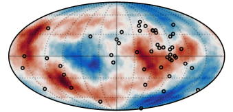
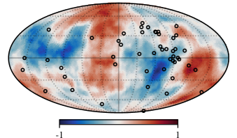
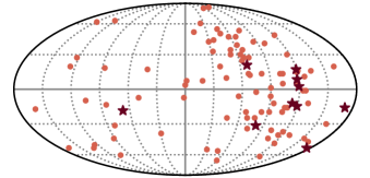
Consider an idealized pta with an infinite number of pulsars smoothly covering the entire sky. In this case, we can make a map of the earth term timing residuals measured at each pulsar. If the time-domain residuals are used, the map will be real and smoothly varying with time. The frequency-domain residuals can be shown as a set of independent complex maps, with one for each frequency bin. Figure 1 shows an example of the latter case for a single frequency bin.
A smooth, full-sky timing residual map can be decomposed into spherical harmonics:
| (10) | ||||
| (11) |
Here represents a spherical harmonic of degree and order , and is its amplitude. The spherical harmonics represent a complete basis for functions defined on the sphere.
Spherical harmonics have several equivalent definitions, and are most commonly defined to be complex-valued. However, the geometry of pulsar sky locations will be more naturally represented using the real-valued spherical harmonics. Equations throughout this paper are appropriate for either real or complex spherical harmonics,222The exception is Equation 26, which is written in terms of the real spherical harmonics. The complex case gains some sign changes associated with the terms. but all figures are made using real spherical harmonics.
If the gwb is a Gaussian random field, each individual will be random and unpredictable, but together they will be statistically described by complex Gaussian distribution. A Gaussian distribution is fully defined by two quantities: the mean and the variance (two-point correlation function). The gw signal has zero mean, so the distribution should as well. This leaves the two-point function as the single quantity which statistically describes the distribution.
The two-point function in harmonic space is known as the angular power spectrum and can be written (e.g. Dodelson, 2003) as:
| (12) |
For a gwb, this becomes (Roebber & Holder, 2017):
| (13) |
The angular power spectrum Equation 12 is mathematically equivalent to the two-point correlation function calculated in the spatial domain (e.g. Dodelson, 2003):
| (14) |
where represents the angle between the two points and on the sky and is the Legendre polynomial of degree . is the frequency power spectrum of the gravitational wave background.
Since Equation 14 is equivalent to Equation 4, the angular power spectrum contains the same information as the Hellings and Downs curve (neglecting pulsar autocorrelations):
| (15) | ||||
| (16) | ||||
| (17) |
This relation (Equation 15) can be thought of as a spherical-harmonic version of a Fourier transform.
Both the Hellings and Downs curve (Equation 17) and the angular correlation function (Equation 13) represent an ensemble average over many different realizations of the gwb. Any single measurement of the two-point function (in a single frequency bin) will differ from the underlying form due to sample variance (see discussion in Roebber & Holder, 2017), but this can be reduced by measuring more frequency bins.
is a steeply decreasing function of ; as expected, most of the power is in the quadrupole moment (), with smaller contributions from higher modes, and none in the monopole or the dipole. This can also be seen in the example timing residual map in Figure 1: the dominant fluctuations are those covering about of the sky, smaller-scale fluctuations are much less important, and fluctuations on scales smaller than are practically absent. The higher-than-quadrupole terms are due to the factor of in Equation 3, and are unrelated to any non-quadrupolar components of the strain.
The quadrupole term of contains nearly all of the signal-to noise of the total gwb, so a successful detection of the gwb will require the detection of . Most contributions to the noise are uncorrelated between pulsars, and should affect all terms of equally.
The spatially correlated noise terms discussed in Section 2, however, have their own characteristic angular power spectra. In both cases, these are very simple: clock errors produce a monopole () signal, and ephemeris errors produce a dipole () signal. Harmonic analysis of the timing residuals naturally separates these spatially correlated noise signals from the gw signal ().
Given this natural separation, why are we concerned that measurements of the gw signal might be contaminated by ephemeris or clock errors? So far, we have assumed that our array of pulsars covers the sky sufficiently completely that we may accurately measure spherical harmonics up to . However, a real pta will have a limited number of pulsars distributed non-uniformly across the sky, and as a result, measurements of spherical harmonics will suffer from convolution with the geometry of the pulsar array. This effect will be the subject of the next section.
4 The mode coupling matrix
We previously assumed an ideal pta which can measure timing residuals at every point on the sky. However, a real pta is limited to only tens of points on the sky: the locations of each pulsar in the array. This section generalizes the results from the previous section to include the effects of a pta which instead sparsely samples the underlying timing residual map.
In an ideal pta, the measured timing residuals form a smooth field, which can be straightforwardly transformed into spherical harmonics, as in Equation 10. This is possible because the spherical harmonics form an orthonormal basis for fields on a sphere. However, for a finite number of pulsars, the spherical harmonics sampled at the locations of the pulsars will no longer form an orthogonal basis function for this space.
Attempting to measure the amplitudes of the standard spherical harmonics will have mixed results: some harmonics will be poorly sampled and power will bleed between different modes. This is particularly a concern if the pulsars are not evenly distributed across the sky, as is the case for the population of known millisecond pulsars (see Figure 2).
The degree to which power from one mode can bleed into another can be represented by a coupling matrix (Peebles, 1973; Gorski, 1994; Wandelt et al., 2001; Mortlock et al., 2002; Hivon et al., 2002; Efstathiou, 2004), which shows how much each spherical harmonic overlaps with all other harmonics:
| (18) | ||||
| (19) |
The window function is used to define the part of the sky measured by pulsars:
| (20) |
where the pulsar sky locations are given by and the weights for each pulsar are given by:
| (21) |
We will discuss the first case (pulsars have different levels of intrinsic noise) in Section 5.3, and otherwise assume the second case (all pulsars are equal).
If complex spherical harmonics are used to calculate , the coupling matrix will be Hermitian. For real spherical harmonics, it will be real and symmetric.
When the integral in Equation 18 is taken over the entire sphere with everywhere, the coupling matrix becomes , and the spherical harmonics are orthonormal once more.
The properties of the coupling matrix determine whether or not we will be able to algebraically disentangle the different modes. When the different harmonics are orthogonal, the coupling matrix is diagonal, and the problem is trivial. In the opposite limit, where all harmonics are maximally entangled, the coupling matrix is singular, and the problem is impossible. In general, if the coupling matrix is well-conditioned (invertible), it should be possible to disentangle the gw signal from dipolar ephemeris and monopolar clock errors.
Since the pta response function , the spherical harmonic transform of the timing residuals will contain gw signal at all , even for a strain signal which is strictly quadrupolar. However, since the majority of the signal is contained in the quadrupole, we will neglect these higher order terms.
Using spherical harmonic product identities, Equation 18 can also be written (e.g. Hivon et al., 2002):
| (26) |
where terms of the form
are known as Wigner 3j symbols, and are closely related to the Clebsch-Gordan coefficients. They can generally not be written in closed form, but obey the following symmetry rules (e.g. Hivon et al., 2002):
| (27) | ||||
| (triangle inequality) | (28) | |||
| (29) |
This form of the coupling matrix is useful, since it is explicitly written in terms of the pulsar sky locations . This will allow us to gain insight into how the latter affects the former (see Section 5.2).
5 PTA configuration and mode coupling
is entirely determined by the properties of the pulsar array. Important properties include the number of pulsars in the array, the spatial distribution of the pulsars, and the quality of each pulsar.
The effects of varying these properties will be illustrated by a set of 6 toy model ptas. The models include arrays with 10 pulsars, with 100 pulsars, and with 10 good pulsars (with weight 1) and 90 poor pulsars (with weight 0.05). The pulsars in each case are generated by random sampling from two spatial distributions: ‘uniform’ and ‘galaxy’.
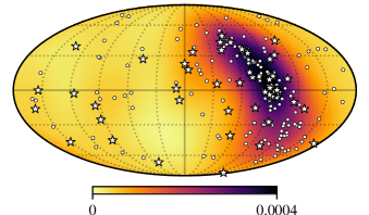
The ‘uniform’ distribution represents the case where every direction is equally likely to contain a pulsar. The ‘galaxy’ distribution is based on the known population of millisecond pulsars, as shown in Figure 2. The distribution was created by selecting millisecond pulsars from the atnf pulsar catalogue (Manchester et al., 2005), removing multiples associated with globular clusters to avoid biasing the distribution towards those sky locations, and smoothing with a Gaussian beam with full width at half maximum of .
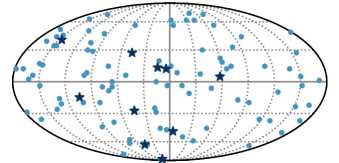
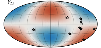
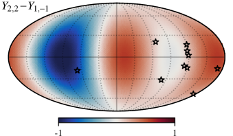
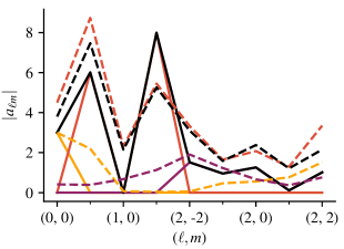
The distribution of pulsars for the ‘uniform’ and ‘galaxy’ cases are shown in Figure 3. The 10-pulsar subsets used for the ‘10 equal pulsars’ and the ‘10 good pulsars’ are marked with dark stars. Examples of harmonics which are not well measured or are coupled to other harmonics are shown in Figure 4. The coupling matrix for each model pta is shown in Figure 5, and their eigenvalues in Figure 6.
5.1 Pulsar number
The first important consideration is the number of pulsars in the array, or the number of points at which the signal is sampled. To successfully disentangle gw signal and spatially correlated clock and ephemeris errors, it will be necessary to measure the (monopole), (dipole), and (quadrupole) moments of the pta response. With too few pulsars, some modes of interest will be poorly sampled, and will not be invertible. This problem is closely related to the Nyquist sampling theorem.
A lower limit on the number of pulsars required can be calculated using a mode-counting argument. There are harmonic modes for every multipole . For a frequency-domain signal, the timing residuals are complex, and all modes are independent. If we assume that the gw signal is approximately band-limited with , we can count the number of modes needed:
| (30) |
Measuring the leading-order term of the gw signal (the quadrupole) and disentangling it from the potentially nonzero monopole and dipole terms would therefore require a minimum of 9 pulsars. Measuring up to the octopole term of the pta response would require a minimum of 16 pulsars.
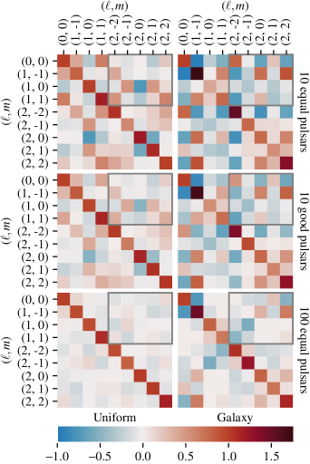
However, larger arrays may perform significantly better. As can be seen in Figure 5, the coupling matrices for the 10-pulsar arrays have large off-diagonal elements, indicating strong coupling, and occasional weak diagonal elements where modes are not well measured (see also Figure 4). These aspects improve for arrays with more pulsars.
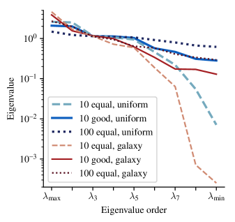
To determine whether the coupling can be removed, we want to know if the coupling matrix is well-conditioned. This can be evaluated by looking at its eigenvalue decomposition, as in Figure 6.
A matrix with at least one zero-valued eigenvalue is singular. If the eigenvalues are nonzero, but very small, it may be possible to numerically invert the matrix, but using the inverse will magnify errors in the data. In this scenario, the matrix is ill-conditioned. A useful figure of merit is the condition number: the ratio between the largest and smallest eigenvalue. When the condition number is close to 1, the matrix is well-conditioned; when it is large, the matrix is ill-conditioned; and when it is infinite, the matrix is singular.
Although the mode-counting argument above suggested that arrays with pulsars should have well-conditioned coupling matrices, the 10-pulsar examples seen in Figure 6 are marginal, particularly in the case of the galaxy-distributed pta. A coupling matrix for a pta with a small number of pulsars can have a wide range of condition numbers, depending on the locations of the different pulsars.
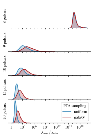
Figure 7 shows the condition number for 1000 different random realizations of arrays with a variable number of pulsars. From the top plot, it is clear that the coupling matrix of any array with 8 pulsars is numerically singular, while for larger arrays, the coupling matrix is not. However, 9- or 10-pulsar arrays show a spread of many orders of magnitude in condition number. Some distributions will be well-conditioned, and some will certainly not. As the number of pulsars increases, the mean and spread decrease, and an array with 20 pulsars, will be more likely to have a well-conditioned coupling matrix.
This result agrees with previous work (Siemens et al., 2013; Taylor et al., 2016) arguing that large arrays are needed to detect a stochastic gwb, albeit for different reasons. However, other researchers (Foster & Backer, 1990; Cornish & Sampson, 2016; Tinto, 2018) have suggested that a 5-pulsar array could be sufficient, which contradicts the 9-pulsar minimum found in this paper.
In the case of Foster & Backer (1990) and Tinto (2018) this is due to a difference in the counting arguments used. Their 5 pulsars can be understood to include 1 pulsar to measure and remove the monopole clock error, 3 pulsars to measure and remove the dipole ephemeris error, and a final pulsar to measure the gwb. However, if the gwb is assumed to have the form of a Gaussian-random quadrupole, it will have 5 independent components, bringing the minimum to 9 pulsars.
On the other hand, Cornish & Sampson (2016) show that small 5-pulsar arrays are adequate for detecting a sufficiently isotropic gwb, in the absence of correlated noise terms. But this does not contradict our results, since they also find that small arrays perform less well for gw signals dominated by small numbers of sources, or in the presence of correlated noise.
The number of pulsars needed for the coupling matrix to be well-conditioned is a useful lower limit on the necessary size of a pta. However, as can be seen in Figure 5, large arrays have less intrinsic coupling between the quadrupole and monopole/dipole modes than small arrays.
This leads to another important threshold: the number of pulsars needed for the coupling between the gw signal and clock/ephemeris error to become unimportant. It happens that the distribution of pulsars across the sky has a significant impact on this threshold, so it will be discussed in the next section.
5.2 Pulsar sky distribution
The second important aspect is the sky distribution of the pulsars. Millisecond pulsars are not located uniformly across the sky (see Figure 2). As a result, the distribution of pulsar separations will not be uniform in , but will be biased towards smaller separations (see figures in Verbiest et al., 2016; Arzoumanian et al., 2018). Furthermore, they are predominantly located in an area which surrounds the center of the galaxy, and is also nearly centered on the ecliptic.
The effect of the pulsar spatial distribution on the form of the coupling matrix is perhaps most clear in Equation 26. In this equation, terms of the form contain information about the pulsars in the array. The Wigner symmetry rules (Equation 28 and Equation 29) determine which terms are important for coupling. In particular, we are interested in coupling between and modes and between and modes. In the first case, harmonics with will contribute, and in the second case, only harmonics with will matter.
This means that any pulsar timing array distribution which has significant dipole, quadrupole, or octopole components will lead to coupling between the quadrupole gw signal and dipole (monopole) ephemeris (clock) error. In particular, the distribution of known millisecond pulsars correlates with the galaxy; from Figure 2, it is clear that distributions of pulsars will naturally tend to cluster around the center of the galaxy, and will therefore have non-negligible dipole, quadrupole, and octopole components. As a result, ptas naively chosen from a collection of the best pulsars will be predisposed towards strong coupling between the quadrupolar signal and the undesired dipole and monopole sources.
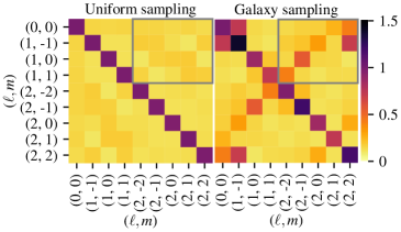
Figure 8, which shows the underlying structure of the amplitudes of the coupling matrices, confirms this. The uniformly-distributed case has no underlying structure, while the galaxy-distributed case has an underlying tendency for certain modes to be coupled.
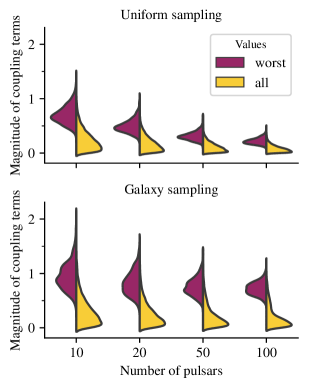
While Figure 8 shows the median coupling matrix for many different random realizations, Figure 9 shows how the amplitudes of the problematic terms of the coupling matrix are distributed across many random realizations. This figure shows that while larger arrays have better coupling matrices, the worst coupling term for galaxy-distributed arrays remains large no matter how many pulsars are included. This worst coupling term has a median value , but can be much higher. From Figure 8, we can see that the strongest coupling term is typically between the mode and the mode.
For galaxy-distributed ptas with many pulsars, most potentially-problematic terms in the coupling matrix are small, but none of the quadrupole modes is free from coupling. The mode shows the least coupling overall ( to the monopole), but it is also the most poorly sampled of the quadrupole modes. These effects can also be seen in the bottom right coupling matrix in Figure 5. With 100 pulsars, this coupling matrix is well-conditioned, but clearly shows the same structure as Figure 8.
Ptas with uniformly distributed pulsars show similarly large couplings when the number of pulsars is small. But as the number of pulsars in the array increases, the overall coupling between quadrupole and monopole/dipole modes decreases, and the matrix becomes increasingly diagonal. With 50 pulsars in the array, the mode with the worst coupling is always , and typical modes are (see Figure 9).
Futuristic ptas with high-quality pulsars may be able to eliminate contamination by solar system ephemeris or clock errors, but only if the pulsars are distributed nearly uniformly across the sky. Current ptas have been constructed to be more isotropic than our naive galaxy-distributed model, but they are not isotropic enough to have low levels of contamination.
In addition to the large-scale distribution of pulsars (dipole–octopole moments), the small-scale distribution of pulsars can also have an effect. Tightly clustered pulsars (separations ) will make highly correlated measurements of the large-scale modes, and so cannot really be considered to be independent. This means that adding an additional pulsar close to one already present will not improve the coupling matrix as well as adding a widely-spaced pulsar would.
As an example, the galaxy-distributed 10-pulsar model (shown in the bottom plot of Figure 3) has two sets of pulsars which are very close to one another. It might be expected to act somewhat like a 7-pulsar array. This is reflected in the eigenvalues of its associated coupling matrix (Figure 6): there is a drop of two orders of magnitude between the seventh- and the eighth-largest eigenvalues.
However, if there are enough widely-separated pulsars in the array, tightly-clustered pulsars may not be a problem. In particular, poor-quality pulsars with large amounts of white or red noise might not be useful on their own. But if there are several of them all sampling the same underlying gw (and ephemeris error) signal, they could act similarly to a single higher-quality pulsar. This effect could be employed in order to build a more uniform array of pulsars, with multiple poor-quality pulsars used to fill large gaps between the better ones.
In summary, a pta must have pulsars in order to be able to separate quadrupolar gw signal from dipolar ephemeris error and monopolar clock error, but there are also requirements on the distribution of those pulsars. Ideally, the pulsars should be arranged uniformly across the sky, with separations . Non-uniformly distributed pulsars will increase the coupling. An array with more closely-spaced pulsars than optimal will need to have more pulsars in order to properly sample the relevant modes.
It is worth noting that this spacing recommendation is different from the spacing that maximizes the detectability of the Hellings and Downs curve. The most important difference is that pulsars with small separations are not useful for improving the coupling matrix. This is because correlations between tightly coupled pulsars may be useful for detecting a correlated signal, but they will be useless for determining whether this correlation is due to a gw signal, an error in the planetary ephemeris, or a clock error.
5.3 Pulsar quality
The final important effect is the quality of different pulsars. This can be treated using the weights defined in Equation 20, so that ‘good’ pulsars have a large weight and ‘bad’ pulsars a small one.
The example for this scenario has the full set of 100 pulsars in Figure 3, but the weights are arranged so that the first 10 have , and the other 90 have . This simulates having a small array of ‘good’ pulsars, with many ‘bad’ pulsars added to it. The weights were chosen to make the effects in Figure 5 and Figure 6 visible.
Comparing the middle row of Figure 5 to the top and bottom shows that the coupling matrix is more similar to the case with 10 equal pulsars than to the case with 100 equal pulsars. We can show this from Equation 19, assuming a simple distribution of weights, as in our example.
Consider two populations of pulsars: ‘good’ pulsars with associated weights and coupling matrix and ‘bad’ pulsars with associated weights and coupling matrix . Since there are more ‘bad’ pulsars than good ones, will typically have stronger diagonal terms, and weaker off-diagonal terms than , although this will depend on the sky distribution of both sets of pulsars.
The contribution of each of these populations to the coupling matrix of the total population (from Equation 19) can be separated:
| (31) |
The overall coupling matrix is a weighted average between the coupling matrices calculated for each population on its own. Unless , ‘good’ pulsars will be more important for the overall form of the coupling matrix. Real ptas tend to have sensitivities which are dominated by a small number of pulsars (e.g. Babak et al., 2016 where 6 out of 41 pulsars contribute more than 90% of the total array’s signal-to-noise squared), so similar results are likely to hold in practice.
Although the form of the coupling matrix is mostly set by the sub-array of ‘good’ pulsars, adding a spatially extended distribution of ‘bad’ pulsars can have a significant effect on the conditioning of the coupling matrix (see Figure 6). The best eigenvalues of are very similar to the best eigenvalues of , but the worst are considerably improved. This suggests that a large number of ‘bad’ pulsars could be used to compensate for not having enough ‘good’ pulsars to measure the desired .
Equation 31 and Weyl’s theorem can be used to place bounds on the amplitude of the smallest eigenvalue for the combined arrays of ‘good’ and ‘bad’ pulsars:
| (32) | ||||
| (33) |
This can be rewritten in terms of the improvement in between the ‘good’ array and the combined array:
| (34) |
where
The difference between the two bounds is related to the spatial distributions of the ‘good’ and the ‘bad’ pulsars. The worst improvement will occur when the two arrays have very similar distributions, and so make degenerate measurements. In this case may be similar in amplitude to , so the improvement can be very small.
By contrast, the best improvement will occur when the two arrays have complementary distributions, so that adding the ‘bad’ pulsars add new information. In this case, since , even a relatively small array of low-weight pulsars can have a significant improvement.
Although adding ‘bad’ pulsars to the ‘good’ ones typically will not significantly change the amount of coupling, they are most likely to be useful when they have a complementary sky distribution to the ‘good’ ones. In this case the off-diagonal terms of their coupling matrices will partially cancel.
In summary, second-rate pulsars are generally less useful for making the sky distribution more uniform, since they have a weaker effect on the coupling matrix, but they are useful for improving the conditioning of the coupling matrix. The best effect will be produced by a collection of ‘bad’ pulsars with nearly the opposite distribution on the sky from the ‘good’ pulsars, in enough numbers that .
6 Correcting for mode coupling
Large numbers of uniformly-distributed pulsars have very little coupling between the gw quadrupole (and higher) terms and spatially-correlated clock and ephemeris errors (monopole and dipole terms). However, since millisecond pulsars do not have a uniform sky distribution, in practice it may not be possible to construct a sensitive pta without this coupling.
It is therefore useful to have techniques for removing the coupling. The standard analysis uses the Hellings and Downs correlation between different pulsars to search for a gwb. An equivalent harmonic space calculation could be made using the angular correlation in Equation 13.
This is both optimal and unbiased if the monopole and dipole terms are both zero. But any single attempted measurement of the gwb where either the monopole or dipole is nonzero will produce biased results (cf. Tiburzi et al., 2016; Vigeland et al., 2018) since power can leak from the monopole or dipole into the gw modes.
Knowledge of the coupling matrix can be used to explicitly remove the contamination, but care must be taken to avoid methods which are unbiased only for an ensemble of observations. This section will explore a single example of how this can be done, but other techniques are possible (cf. Tinto, 2018).
6.1 Orthogonalized spherical harmonics
One way to deal with the coupling is to build a new set of orthogonal basis functions based on the spherical harmonics. As shown in Gorski (1994) and Mortlock et al. (2002) in the context of analysis of the cosmic microwave background anisotropies, this approach allows us to identify and excise components which are contaminated by the noisy monopole and dipole. This section and the next will apply their strategy in the context of pulsar timing arrays. For mathematical ease, the notation of the previous sections will be used interchangeably with linear algebra notation: .
The orthogonalization will be performed using a Cholesky decomposition of the coupling matrix:
| (35) |
where is a lower-triangular matrix, and represents the Hermitian transpose of .
The new orthogonalized harmonics are given by:
| (36) |
By construction, they are orthonormal on the space of the pulsar sky positions:
| (37) |
The new coefficients are similarly related to the true harmonic coefficients:
| (38) |
and can be estimated from the measured timing residuals (cf. Equation 11):
| (39) |
The spherical harmonics are best described with two indices , but the transformation in Equation 36 doesn’t preserve these symmetries. As a result, the orthogonalized spherical harmonics have only a single index (denoted hereafter by or ), which is related to the components of .
Since the transformation in Equation 38 is based on a Cholesky decomposition, is upper-triangular. This means that the components of contain contributions from a decreasing number of modes of .
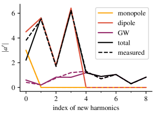
The first term of , , is made up of contributions from all . If the components of are arranged in ascending order of the ’s, then will contain contributions from all the except for the monopole. Similarly, the next three terms of progressively drop the dipole terms. Therefore, only the first four components of contain any contribution from the monopole and dipole modes
By dropping those first four terms, we can cleanly separate the gw signal from the effect of the ephemeris and clock errors (see Figure 10). Since the ambiguous components are also dropped, some amount of signal will be lost. This can be calculated (on average) from the form of . In general, coupling matrices with large coupling terms and with larger condition numbers will lose more signal.
This process can be visualized as a switch to a new basis of functions which are built of spherical harmonics. This new basis consists of (1) functions which contain the well-measured components of the quadrupole and (2) functions which contain the poorly-measured components of the quadrupole plus the monopole and dipole terms. For an array with a lot of coupling, functions of type (1) will not cover much of the sky, and so a significant amount of signal will be lost. By contrast, for an array with a nearly diagonal coupling matrix, functions of type (1) will approximately recover the quadrupole spherical harmonics, and very little signal will be lost.
Note that in ecliptic coordinates, we can expect that the ephemeris error will only contaminate the modes, so we could limit ourselves to removing the contributions from only three modes: , , and . This would reduce the number of ambiguous modes, so that more signal could be recovered.
This technique is related to the one described by Tinto (2018), but leads to a very different set of uncontaminated modes, with very different covariance properties. There are also other techniques that can be used to construct orthogonal modes from spherical harmonics. The Cholesky decomposition was used for simplicity in constructing the clean modes , but there are many other options. Mortlock et al. (2002) discusses this problem more generally, including the case of a singular value decomposition, as well as techniques for extending the analysis to higher , where the coupling matrix becomes singular.
6.2 Likelihood analysis
The vector can be thought of as a set of five linear combinations of the pulsar timing residuals, each of which is insensitive to the noisy monopole and dipole terms (note that we have now dropped the four contaminated modes). In this section, we will discuss the statistical properties of which are needed for gwb searches.
For a Gaussian gwb, the spherical harmonic amplitudes are by definition normally distributed. The amplitudes of the orthogonalized spherical harmonics can each be written as a sum of components. Therefore, the new amplitudes are also Gaussian random variables:
| (40) |
where is the number of modes. If and all monopole and dipole modes are removed, . The covariance matrix can be separated into a signal component and pulsar noise component: .
The signal covariance matrix can be defined in terms of the coefficients of the orthogonalized harmonics:
| (41) |
where and now represent the index of the orthogonal modes where all monopole and dipole terms have been dropped. The second line is found using Equation 12 and noting that is the same for all at fixed .
In a full-sky analysis, the orthogonality of the spherical harmonics means that is diagonal (with amplitudes given by ). However, this is not generally the case for the orthogonalized spherical harmonics. As the array becomes larger and more uniform, the coupling matrix will approach the identity matrix, and will become approximately uniform.
Assuming that the noise in each pulsar is given by and is uncorrelated with other pulsars, the noise covariance matrix can be written:
| (42) | ||||
| (43) |
This is diagonal and exactly equal to the identity matrix if all pulsars are identical, or if the pulsar weights are equal to the inverse variance of their noise: .
7 Discussion
The form of the antenna response function ensures that pta searches for gws have an inherently geometric component. This is fortunate, since it gives us a way to decouple the gw signal from correlated noise sources such as planetary ephemeris errors and clock errors.
A natural space in which to do this is provided by a spherical harmonic analysis of the pulsar timing residuals. In this space, gws appear as quadrupole and higher order terms, while ephemeris errors appear as dipole terms, and clock errors appear as a monopole.
However, real ptas are composed of a moderate number of pulsars with varying intrinsic noise levels, distributed nonuniformly across the sky. Attempts to measure the different modes are therefore subject to aliasing-type effects, and the measured quadrupole gw signal may be contaminated by the clock error monopole and ephemeris error dipole.
This contamination can be quantified in terms of a coupling matrix, which measures the extent to which different spherical harmonics are non-orthogonal for a given array of pulsars. The coupling matrix depends only on the spatial arrangement and noise properties of the pulsars in the array, and so provides a means to assess the degree to which contamination by ephemeris errors or clock errors is likely to be an issue for a particular configuration of pulsars.
Measuring the monopole, dipole, and quadrupole modes requires an array with a minimum of 9 pulsars, but such arrays are typically subject to considerable coupling between the gw signal and ephemeris or clock errors. The arrays with the fewest coupling problems are those with many isotropic, high-quality pulsars. However, since the underlying distribution of millisecond pulsars is anisotropic, future ptas will probably still experience significant amounts of coupling.
A biased array can be made less biased by keeping only the best pulsars from the region around galactic center and by adding clusters of second-rate pulsars wherever possible in the undersampled regions. In particular, covering the ecliptic plane is especially useful for minimizing coupling with the dipole modes most likely to be induced by ephemeris errors.
The distribution of pulsars which allows the gw signal to be most cleanly separated from the clock and ephemeris errors is not the same as the one which is most sensitive to detecting gws, since the latter case favors closely-spaced pulsars, which tend to increase coupling.
A pta with significant coupling will need to correct for that coupling. If the array contains a large enough number of pulsars, the coupling matrix will be invertible, and the coupling can be removed algebraically. This paper and Tinto (2018) present different examples of how the analysis can be done in a space which nulls contributions from the monopole and dipole terms. These algebraic techniques are complementary to physical models such as the planetary ephemeris model BayesEphem (Arzoumanian et al., 2018), .
Throughout this paper, we have assumed that ephemeris and clock errors produce pure monopolar and dipolar correlations between all pulsars in the array, but this will be more complicated in reality. In particular, timing residuals from different pulsars are irregularly sampled, there are gaps in the timing of certain pulsars, and new pulsars are occasionally added to the array. As a result, a real pta cannot be treated as a static collection of pulsars, and a frequency-domain analysis becomes difficult.
It is possible to extend the analysis of this paper to the time domain. The time-domain coupling matrix can be calculated with Equation 19, using real spherical harmonics and time-varying pulsar positions and weights. The single coupling matrix that we have been considering becomes instead a series of different coupling matrices as pulsars are added and subtracted. As a result, the degree of contamination by ephemeris and clock errors will also vary as a function of time. If the analysis above is followed, this will also lead to a choice of which is not smoothly varying.
The analysis presented in this paper has also treated only the case where the gwb is an isotropic Gaussian random field. This may be an oversimplification. It is plausible that strong individual gw sources will dominate the signal in some frequency bins (Sesana et al., 2008; Ravi et al., 2012; Roebber et al., 2016). Although there are better means to detect single sources (e.g. Lee et al., 2011; Boyle & Pen, 2012; Babak & Sesana, 2012; Zhu et al., 2016; Goldstein et al., 2018), their presence should not significantly bias our analysis (cf. Cornish & Sampson, 2016).
Single sources of gws also produce Hellings and Downs correlations between pulsars, and, equivalently, the same angular power spectrum as in Equation 13. For multiple sources, as with individual realizations of the stochastic gwb, this correlation represents an ensemble average and does not hold exactly (Roebber & Holder, 2017).
The primary difference between these cases is that for a stochastic gwb, the power in each multipole is random and uncorrelated, while for a gw signal produced by a few loud sources, the power in different multipoles becomes correlated due to interference between the pulsar antenna response to each source. These correlations appear as small ripples in the angular power spectrum (Roebber & Holder, 2017). Since the underlying form of the angular power spectrum is similar in all cases, it will almost always be appropriate to approximate it as a quadrupole. As a result, the technique described in this paper should work even when our assumptions of a statistically isotropic and Gaussian random gwb is violated by the presence of a few loud sources.
Large-scale anisotropies in the distribution of gw sources (Mingarelli et al., 2013; Taylor & Gair, 2013), however, could produce a gwb with a very different power spectrum. In this case, the assumption that the gw signal is largely contained in the quadrupole modes will no longer hold. However, this scenario is unlikely in practice, as it represents a significant departure from cosmological isotropy.
The problems discussed in this paper will also affect astrometric gw searches using Gaia and similar experiments (Klioner, 2018; O’Beirne & Cornish, 2018; Darling et al., 2018; Mihaylov et al., 2018). Gaia observes many stars, but star locations are biased towards the direction of the galaxy, so similar coupling problems will arise.
Similarly, measurements of just the clock (Hobbs et al., 2012) or the planetary ephemeris (Champion et al., 2010) errors could experience significant coupling with the other effect or with gws. A variant of the method described here may be useful for attempts to measure these individual quantities.
Although the problem of ephemeris errors is not trivial, it is solvable, especially for future arrays with many high-quality pulsars.
References
- Arzoumanian et al. (2018) Arzoumanian, Z., Baker, P. T., Brazier, A., et al. 2018, ApJ, 859, 47
- Babak & Sesana (2012) Babak, S., & Sesana, A. 2012, Phys. Rev. D, 85, 044034
- Babak et al. (2016) Babak, S., Petiteau, A., Sesana, A., et al. 2016, MNRAS, 455, 1665
- Begelman et al. (1980) Begelman, M. C., Blandford, R. D., & Rees, M. J. 1980, Nature, 287, 307
- Boyle & Pen (2012) Boyle, L., & Pen, U.-L. 2012, Phys. Rev. D, 86, 124028
- Champion et al. (2010) Champion, D. J., Hobbs, G. B., Manchester, R. N., et al. 2010, ApJ, 720, L201
- Chen et al. (2018) Chen, S., Sesana, A., & Conselice, C. J. 2018, arXiv:1810.04184
- Cordes (2013) Cordes, J. M. 2013, Classical and Quantum Gravity, 30, 224002
- Cornish & Sampson (2016) Cornish, N. J., & Sampson, L. 2016, Phys. Rev. D, 93, 104047
- Darling et al. (2018) Darling, J., Truebenbach, A. E., & Paine, J. 2018, ApJ, 861, 113
- Dodelson (2003) Dodelson, S. 2003, Modern cosmology (Academic Press)
- Edwards et al. (2006) Edwards, R. T., Hobbs, G. B., & Manchester, R. N. 2006, MNRAS, 372, 1549
- Efstathiou (2004) Efstathiou, G. 2004, MNRAS, 349, 603
- Foster & Backer (1990) Foster, R. S., & Backer, D. C. 1990, ApJ, 361, 300
- Gair et al. (2014) Gair, J., Romano, J. D., Taylor, S., & Mingarelli, C. M. F. 2014, Phys. Rev. D, 90, 082001
- Goldstein et al. (2018) Goldstein, J. M., Veitch, J., Sesana, A., & Vecchio, A. 2018, MNRAS, 477, 5447
- Gorski (1994) Gorski, K. M. 1994, ApJ, 430, L85
- Górski et al. (2005) Górski, K. M., Hivon, E., Banday, A. J., et al. 2005, ApJ, 622, 759
- Hellings & Downs (1983) Hellings, R. W., & Downs, G. S. 1983, ApJ, 265, L39
- Hivon et al. (2002) Hivon, E., Górski, K. M., Netterfield, C. B., et al. 2002, ApJ, 567, 2
- Hobbs & Dai (2017) Hobbs, G., & Dai, S. 2017, arXiv:1707.01615
- Hobbs et al. (2012) Hobbs, G., Coles, W., Manchester, R. N., et al. 2012, MNRAS, 427, 2780
- Hunter (2007) Hunter, J. D. 2007, Computing In Science & Engineering, 9, 90
- Jones et al. (2001–present) Jones, E., Oliphant, T., Peterson, P., & et al. 2001–present, SciPy: Open source scientific tools for Python
- Joshi et al. (2018) Joshi, B. C., Arumugasamy, P., Bagchi, M., et al. 2018, Journal of Astrophysics and Astronomy, 39, 51
- Keane et al. (2015) Keane, E., Bhattacharyya, B., Kramer, M., et al. 2015, in Advancing Astrophysics with the Square Kilometre Array (AASKA14), 40
- Klioner (2018) Klioner, S. A. 2018, Classical and Quantum Gravity, 35, 045005
- Lasky et al. (2016) Lasky, P. D., Mingarelli, C. M. F., Smith, T. L., et al. 2016, Physical Review X, 6, 011035
- Lazio et al. (2018) Lazio, T. J. W., Bhaskaran, S., Cutler, C., et al. 2018, in IAU Symposium, Vol. 337, Pulsar Astrophysics the Next Fifty Years, ed. P. Weltevrede, B. B. P. Perera, L. L. Preston, & S. Sanidas, 150
- Lee (2016) Lee, K. J. 2016, in Astronomical Society of the Pacific Conference Series, Vol. 502, Frontiers in Radio Astronomy and FAST Early Sciences Symposium 2015, ed. L. Qain & D. Li, 19
- Lee et al. (2011) Lee, K. J., Wex, N., Kramer, M., et al. 2011, MNRAS, 414, 3251
- Lentati et al. (2013) Lentati, L., Alexander, P., Hobson, M. P., et al. 2013, Phys. Rev. D, 87, 104021
- Lentati et al. (2015) Lentati, L., Taylor, S. R., Mingarelli, C. M. F., et al. 2015, MNRAS, 453, 2576
- Lorimer (2008) Lorimer, D. R. 2008, Living Reviews in Relativity, 11, arXiv:0811.0762
- Manchester et al. (2005) Manchester, R. N., Hobbs, G. B., Teoh, A., & Hobbs, M. 2005, AJ, 129, 1993
- McKinney (2010) McKinney, W. 2010, in Proceedings of the 9th Python in Science Conference, ed. S. van der Walt & J. Millman, 51
- Mihaylov et al. (2018) Mihaylov, D. P., Moore, C. J., Gair, J. R., Lasenby, A., & Gilmore, G. 2018, Phys. Rev. D, 97, 124058
- Mingarelli et al. (2013) Mingarelli, C. M. F., Sidery, T., Mandel, I., & Vecchio, A. 2013, Phys. Rev. D, 88, 062005
- Mortlock et al. (2002) Mortlock, D. J., Challinor, A. D., & Hobson, M. P. 2002, MNRAS, 330, 405
- O’Beirne & Cornish (2018) O’Beirne, L., & Cornish, N. J. 2018, Phys. Rev. D, 98, 024020
- Peebles (1973) Peebles, P. J. E. 1973, ApJ, 185, 413
- Rajagopal & Romani (1995) Rajagopal, M., & Romani, R. W. 1995, ApJ, 446, 543
- Ravi et al. (2012) Ravi, V., Wyithe, J. S. B., Hobbs, G., et al. 2012, ApJ, 761, 84
- Roebber & Holder (2017) Roebber, E., & Holder, G. 2017, ApJ, 835, 21
- Roebber et al. (2016) Roebber, E., Holder, G., Holz, D. E., & Warren, M. 2016, ApJ, 819, 163
- Romano & Cornish (2017) Romano, J. D., & Cornish, N. J. 2017, Living Reviews in Relativity, 20, 2
- Sesana et al. (2008) Sesana, A., Vecchio, A., & Colacino, C. N. 2008, MNRAS, 390, 192
- Shannon et al. (2015) Shannon, R. M., Ravi, V., Lentati, L. T., et al. 2015, Science, 349, 1522
- Siemens et al. (2013) Siemens, X., Ellis, J., Jenet, F., & Romano, J. D. 2013, Classical and Quantum Gravity, 30, 224015
- Taylor & Gair (2013) Taylor, S. R., & Gair, J. R. 2013, Phys. Rev. D, 88, 084001
- Taylor et al. (2017a) Taylor, S. R., Lentati, L., Babak, S., et al. 2017a, Phys. Rev. D, 95, 042002
- Taylor et al. (2017b) Taylor, S. R., Simon, J., & Sampson, L. 2017b, Phys. Rev. Lett., 118, 181102
- Taylor et al. (2016) Taylor, S. R., Vallisneri, M., Ellis, J. A., et al. 2016, ApJ, 819, L6
- Tiburzi et al. (2016) Tiburzi, C., Hobbs, G., Kerr, M., et al. 2016, MNRAS, 455, 4339
- Tinto (2018) Tinto, M. 2018, Phys. Rev. D, 97, 084047
- van der Walt et al. (2011) van der Walt, S., Colbert, S. C., & Varoquaux, G. 2011, Computing in Science & Engineering, 13, 22
- van Haasteren & Vallisneri (2014) van Haasteren, R., & Vallisneri, M. 2014, Phys. Rev. D, 90, 104012
- van Haasteren & Vallisneri (2015) —. 2015, MNRAS, 446, 1170
- Verbiest et al. (2016) Verbiest, J. P. W., Lentati, L., Hobbs, G., et al. 2016, MNRAS, 458, 1267
- Vigeland et al. (2018) Vigeland, S. J., Islo, K., Taylor, S. R., & Ellis, J. A. 2018, Phys. Rev. D, 98, 044003
- Wandelt et al. (2001) Wandelt, B. D., Hivon, E., & Górski, K. M. 2001, Phys. Rev. D, 64, 083003
- Waskom et al. (2017) Waskom, M., Botvinnik, O., O’Kane, D., et al. 2017, mwaskom/seaborn: v0.8.1
- Zhu et al. (2016) Zhu, X.-J., Wen, L., Xiong, J., et al. 2016, MNRAS, 461, 1317