A Wide-orbit Exoplanet OGLE-2012-BLG-0838Lb

Abstract

We present the discovery of a planet on a very wide orbit in the microlensing event OGLE-2012-BLG-0838. The signal of the planet is well separated from the main peak of the event and the planet-star projected separation is found to be twice the Einstein ring radius, which corresponds to a projected separation of $\approx 4~{}{\rm AU}$. Similar planets around low-mass stars are very hard to find using any technique other than microlensing. We discuss microlensing model fitting in detail and discuss the prospects for measuring the mass and distance of the lens system directly.

1 Introduction

The exoplanets known today show a large degree of diversity. For example, we now know a planetary system orbiting a pulsar (PSR1257+12; Wolszczan & Frail, 1992), extremely short-period planets (55 Cnc e; Winn et al., 2011), planets with extremely high surface temperatures (KELT-9b; Gaudi et al., 2017), rocky planets in the habitable zone (Kepler-186f; Quintana et al., 2014), a gas giant planet orbiting a brown dwarf (2M1207b; Chauvin et al., 2004), and an Earth-mass planet around an ultra-cool dwarf (OGLE-2016-BLG-1195; Shvartzvald et al., 2017), to name a few. These planets have been discovered using a few different detection techniques, and each technique has distinct capabilities and limitations. By far the largest number of planets have been discovered using the transit technique, and in particular the yield of planets from Kepler, the first mission to statistically explore the population of exoplanets over a broad region of parameter space, was notably high (Coughlin et al., 2016). Kepler exoplanets are on orbits similar to the inner planets in the Solar System and in many cases are more compact than that of Mercury. The longest-period confirmed transiting exoplanets are: Kepler-1647b (1108 days; Kostov et al., 2016), Kepler-167e (1071 days; Kipping et al., 2016), and Kepler-1654b (1048 days; Beichman et al., 2018). The orbital periods of these planets are shorter than the orbital periods of all Solar System gas and ice giants. The lack of a large number of the long-period planets hampers our understanding of the formation of planetary systems as a whole and our ability to place the Solar System in the context of known exoplanetary systems in particular.

The main reason for this unsatisfactory situation is that different planet detection techniques have different sensitivities to the wide-orbit planets. For giant planets, the radial velocity (RV) technique is intrinsically limited by the length of the time-baseline of the RV surveys themselves (Kane, 2011; Sahlmann et al., 2016; Wittenmyer et al., 2017). For example, only recently did Blunt et al. (2019) report the detection of a $3M_{\rm Jup}$ minimum mass object on a $74^{+43}_{-22}~{}{\rm yr}$ long highly eccentric orbit via RVs, and in this case the detection required a fairly fortuitous alignment of the orbit of the planet. In particular, the RV data taken during periastron passage of the planet exhibited a signal that is highly unlikely to be produced by other astronomical phenomenon. The limit set by the long-term stability of the spectrographs makes detection of long-period Neptune-mass planets much more difficult than long-period Jupiter-mass planets: the RV signals are $0.5~{}{\rm m\,s^{-1}}$ and $9~{}{\rm m\,s^{-1}}$, respectively, for a Neptune-mass and a Jupiter-mass planet on a $10~{}{\rm AU}$ edge-on orbit around $1~{}M_{\odot}$ star. Astrometric detection of planets on relatively wide orbits (semi-major axis up to $5\textup{--}6~{}{\rm AU}$) can be done using Gaia data or by combining Gaia and Hipparcos data (Perryman et al., 2014; Snellen & Brown, 2018), but the astrometric technique is also only sensitive down to Jupiter-mass objects for most stars. Gaia mission can be extended from nominal $5~{}{\rm yr}$ up to $10~{}{\rm yr}$ and this will increase number of detected planets by a factor of $3\textup{--}4$ (Perryman et al., 2014). Extension of Gaia mission improves sensitivity to wider-orbit and lower-mass planets, but still predicted detections are smaller than the orbit of Saturn. Combination of RV and astrometric techniques improves constraints on the orbital period (Eisner & Kulkarni, 2002; Feng et al., 2019), but fundamental limitations given earlier still apply.

There are two planet detection techniques that find wide-orbit planets: direct imaging and microlensing. Current direct imaging surveys (Baron et al., 2019; Nielsen et al., 2019) can detect planets with separations from $\approx 5~{}{\rm AU}$ to thousnads of AU and more massive than $\approx 2$ Jupiter masses. While the separation ranges for direct imaging and microlensing planets overlap, there are significant differences. Direct imaging discovers self-luminous planets around nearby young stars, and allows follow-up studies of these directly detected objects, including spectroscopy (Bowler, 2016). Contarary, the microlensining planets orbit old stars and there is no possibility for spectroscopy of these planets. Comparison of statical properties of direct imaging and microlensing planets should give constraints on planet migration.

The microlensing technique is sensitive to planetary systems that are a few kpc away, and mostly probe the planetary population orbiting the most numerous, low-mass (and hence mostly old) stars. The ongoing microlensing surveys are sensitive to planet/star mass ratios smaller than $10^{-3}$ even for wide-orbit planets. In fact, the widest-orbit microlensing planet has mass ratio of $2.4\times 10^{-4}$ (OGLE-2008-BLG-092LAb; Poleski et al., 2014). Microlensing can probe Neptune-mass planets, even for planets that have no detectable stellar host and thus may be unbound (Mróz et al., 2018).

It is important to combine the constraints of both the wide-orbit and the free-floating planets (Mróz et al., 2017) in order to fully understand the formation and evolution of planetary systems. The bound-planet parameters that are readily measured for microlensing are the mass ratio ($q$) and the projected separation ($s$) in units of the Einstein ring radius ($\theta_{\rm E}$). The microlensing planets with the widest orbits are OGLE-2008-BLG-092LAb ($s=5.3$; Poleski et al., 2014), OGLE-2011-BLG-0173Lb ($s=4.6$; Poleski et al., 2018), and KMT-2016-BLG-1107Lb ($s=3.0$; Hwang et al., 2019) – see discussion in Poleski et al. (2018). There are only a few more planets with $s>2$. For a typical configuration, $\theta_{\rm E}$ corresponds to around $2.5~{}{\rm AU}$. Hence, the three widest-orbit planets are at projected separations from $7$ to $15~{}{\rm AU}$. The distribution of microlensing planets as a whole has already been studied statistically (e.g., Gould et al., 2010; Cassan et al., 2012; Suzuki et al., 2016; Udalski et al., 2018), but the statistical properties of the wide-orbit planets have not yet been comprehensively analyzed, partly due to the small number of known such systems.

The large sample of wide-orbit planets is important for understanding formation of planetary systems. We have detailed knowledge about Uranus and Neptune, but explaining their formation is challenging. Pollack et al. (1996) showed that in-situ formation in standard core-accretion model cannot reproduce properties of Uranus and Neptune. Three major theoretical approaches to formation of Solar System ice giants are: migration from closer orbits (Thommes et al., 1999; Tsiganis et al., 2005), pebble accretion (Lambrechts et al., 2014; Venturini & Helled, 2017), and collisions of planetary embryos (Izidoro et al., 2015). At this point, none of these theories are favoured.

Here we present the discovery of a wide-orbit exoplanet OGLE-2012-BLG-0838Lb. A short-duration anomaly is observed well before the main peak of the event and points to an event with $s=2.1$. The wide-orbit planet interpretation is confirmed by detailed modeling. The planetary anomaly was found in pure survey observations by the Optical Gravitational Lensing Experiment (OGLE; Udalski et al., 2015), i.e., the planet detection did not depend on targeted follow-up photometry. This means that the planet can be included in future statistical studies of the wide-orbit planets. For OGLE-2012-BLG-0838, high-resolution imaging and satellite imaging were collected, which helps to constrain the planet properties.

In the next section, we present the data collected for OGLE-2012-BLG-0838. We describe the model fitting in Section 3. In Section 4, we analyze current constraints on the physical properties of the system. We summarize the paper in Section 5.

2 Observations

2.1 OGLE photometry

OGLE is a large scale photometric survey. It is currently in its fourth phase (OGLE-IV) and operates a 1.3-m telescope at Las Campanas Observatory (Chile) that is equipped with a 32-CCD chip camera (256M pixels in total). The camera field of view is $1.4~{}{\rm deg^{2}}$, and the pixel scale is $0\farcs 26$. OGLE bulge observations are performed in the $I$ band, and we use only these to fit the microlensing model. When the anomaly occurred, the field of OGLE-2012-BLG-0838 was observed once per one or two nights as part of bulge survey observations aiming at finding ongoing microlensing events. This cadence is not enough for characterizing planetary anomalies in most cases, but gives targets for follow-up photometric observations. For OGLE-2012-BLG-0838 anomaly, there is a single epoch that deviates by more than $1~{}{\rm mag}$ and four epochs that deviate by less than $0.25~{}{\rm mag}$. There are 20 OGLE fields that are observed with higher cadence. For the OGLE-2012-BLG-0838 field and CCD camera chip (#32), the median seeing is $1\farcs 46$, which is slightly higher than for the same chip in higher-cadence bulge fields ($\approx 1\farcs 35$). Additional lower cadence $V$-band data taken in survey mode on the target exist, but do not cover the anomaly, and we use them only to characterize the source star. Photometry of the OGLE data is performed using difference image analysis (DIA; Alard, 2000; Woźniak, 2000). We corrected the native photometric uncertainties following Skowron et al. (2016). We use data from 2012 as well as 2011, which constrain the baseline brightness. For a more detailed description of the OGLE survey, see Udalski et al. (2008) and Udalski et al. (2015).

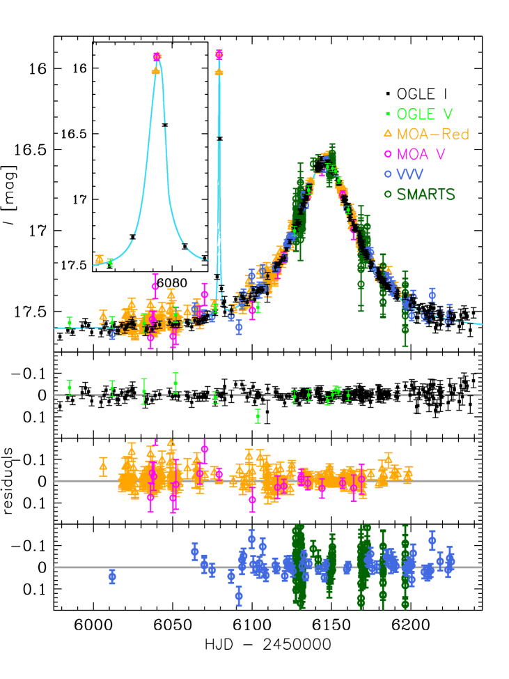
The search for microlensing events in the OGLE data is performed daily (Udalski, 2003). The event OGLE-2012-BLG-0838 was discovered on ${\rm HJD^{\prime}}\tbond{\rm HJD}-2450000=6082$, i.e., after the anomaly was over (see Figure 1). The planetary nature of the anomaly was first suggested on ${\rm HJD^{\prime}}=6126.403$ (by A. U.), and subsequently the planetary models were fitted (by C. H.). Event coordinates are ${\rm R.A.}=18^{\rm h}12^{\rm m}00\fs 74$ and ${\rm Dec.}=-25\arcdeg 42\arcmin 41\farcs 8$, which translate to $l=5\fdg 720$ and $b=-3\fdg 472$. The baseline brightness in the standard photometric system is: $I=17.610~{}{\rm mag}$ and $(V-I)=1.851~{}{\rm mag}$ (Szymański et al., 2011).

Figure 1: Light curve of OGLE-2012-BLG-0838 and the best-fitting model top panel. All avaialable photometry is shown. The inset zooms in on the anomaly. The lower three panels show residuals (two datasets per panel).

2.2 MOA photometry

The Microlensing Observations in Astrophysics (MOA; Bond et al., 2001; Sumi et al., 2003) collaboration also conducts a microlensing survey toward the bulge by using the MOA-II 1.8-m telescope. The telescope is located at Mt John University Observatory (New Zealand). The camera used is the MOA-cam3 (Sako et al., 2008). It is mounted on the prime focus of the telescope and has field of view of $2.2~{}{\rm deg}^{2}$, which enables high-cadence observations. Unfortunately, the event OGLE-2012-BLG-0838 is located in the gap between CCD chips #3 and #8 of gb18 field in the reference image. The reference images are used for the DIA pipeline (Bond et al., 2001) to find and alert new microlensing events. Thus, the event was not discovered by the MOA collaboration and it was thought that MOA has no data for OGLE-2012-BLG-0838. The MOA data were re-checked after the initial version of this paper was submitted and it was revealed that the target is only $3\arcsec$ away from the edge of CCD chip #3. Since the typical telescope pointing accuracy is larger than $3\arcsec$ and this field is observed in survey mode every 50 minutes with the custom MOA-Red filter, we were able to derive the MOA light curve which is dense enough to cover the anomaly. In addition to the MOA-Red data, occasional $V$-band data were also obtained. Over the anomaly, there are two MOA-Red epochs and a single $V$-band epoch and all these data come from a single night. The MOA data were reduced using the MOA’s implementation of the DIA pipeline. Also, the MOA data were corrected for the possible effects of seeing, airmass, and differential refraction (Bond et al., 2017) by fitting to the baseline data two fifth-order polynomials of seeing and hour angle. The resulting correction was applied to all the MOA data and improved the baseline by $\Delta\chi^{2}=694$ for 1344 datapoints. The amplitude of variations are $\pm 300$ MOA flux counts, or $\pm 0.03~{}{\rm mag}$ at the baseline. Similar trends are not seen in OGLE data. We note that the 3 MOA data points taken during the anomaly show consistent shape of the anomaly. In order to account for the underestimated uncertainties, we multiply them by $1.67$ and $1.55$ for MOA-Red and $V$ band, respectively. These values were selected so that $\chi^{2}/{\rm dof}\approx 1$ for an initially fitted model. The MOA baseline photometry shows trends on timescales on the order of one year, thus we restricted MOA data to 2012. Similar trends were seen in previously published events and in the present case the photometry can be additionally affected by the location of the event very close to the CCD chip edge.

2.3 EPOXI imaging

Thanks to the early recognition of its anomaly, OGLE-2012-BLG-0838 was scheduled for observations with the EPOXI mission, which was the repurposed Deep Impact spacecraft (Hampton et al., 2005). There are 6516 images collected between ${\rm HJD^{\prime}}=6136$ and $6150$. The EPOXI images are out of focus, each star produces a doughnut-shaped image, and the PSF changes with the color of the star. In the dense stellar fields of the Galactic bulge, the images of many stars are overlapping, which hinders photometric analysis. Thus the OGLE-2012-BLG-0838 EPOXI data have not yet been reduced. For a reduction and analysis of the EPOXI data for a different event, see Muraki et al. (2011). Previous experience with photometric reduction of Spitzer and K2 bulge images (undersampled in both cases) shows that photometric reduction of bulge images taken by satellite missions requires special efforts (Calchi Novati et al., 2015; Zhu et al., 2017; Poleski et al., 2019).

2.4 VVV photometry

The Variables in the Via Lactea (VVV) survey (Minniti et al., 2010) observed the Galactic bulge between 2010 and 2015 using the near-infrared 4-m VISTA telescope situated at the Paranal Observatory (Chile). VVV took most of its observations in the $K_{s}$ band. The event OGLE-2012-BLG-0838 is detectable in VVV data, but no useful data were taken during or close to the anomaly. The epoch closest to the anomaly was secured under non-photometric conditions. Hence, the VVV $K_{s}$-band data do not usefully constrain the binary-lens microlensing model, and we use them only to derive the source properties. Photometry was extracted using a PSF-fitting technique. From the VVV data we derive a baseline of $K_{s}=15.190~{}{\rm mag}$.

2.5 SMARTS photometry

Immediately following A. U.’s planetary alert (HJD’ = 6126.403), the Microlensing Follow Up Network ($\mu$FUN) initiated observations using the ANDICAM dual-beam optical-IR camera (DePoy et al., 2003) on the SMARTS 1.3m telescope at Cerro Tololo InterAmerican Observatory (CTIO, Chile). The sole purpose of these observations was to characterize the source, primarily to measure the $H$-band source flux in order to compare to possible future high-resolution adaptive optics imaging. During these $H$-band observations using the IR channel, the optical channel was used to obtain $V$ and $I$ data as a backup for the unlikely possibility of problems with the OGLE $V$-band data. However, as anticipated, there were no such problems. Hence, only the $H$-band data are used in the present analysis. Because the observations began before the main peak, they covered a complete range of magnifications of the main subevent from near-baseline to peak, which is the main guarantee for an accurate measurement of the source flux. The data were reduced using DoPhot (Schechter et al., 1993). The zero-point of the photometry was calibrated using $154$ nearby stars with VVV photometry. The difference between VVV photometry and SMARTS instrumental magnitudes shows a linear dependence on the magnitude itself and we take this effect into account in the zero-point calibration. The calibration has an uncertainty of $0.053~{}{\rm mag}$. There were a total of $205$ $H$-band observations in 10 dither or 5 dither groups at a total of $21$ epoch, of which $150$ observations were successfully reduced. Median seeing of SMARTS data is $1\farcs 2$.

2.6 Magellan adaptive optics imaging

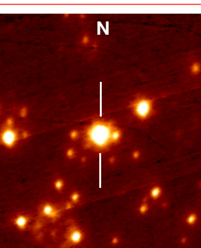
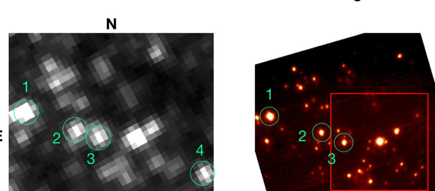
The $H$-band high-resolution images of the OGLE-2012-BLG-0838 field were taken on ${\rm HJD^{\prime}}=6766$, with Magellan Adaptive Optics system (MagAO; Close et al., 2012; Males et al., 2014; Morzinski et al., 2014) on the 6.5-m Clay Telescope at Las Camapanas Observatory (Chile). We used the Clio Wide camera, which has a plate scale of $27.49~{}{\rm mas}$ and a field of view of $14\arcsec\times 28\arcsec$. The integration time for an individual science exposure was $30~{}{\rm seconds}$, and we took ten sets of images with four dithers for each set. Individual dithered frames were astrometrically aligned using the positions of the 10 bright isolated stars, and then the aligned and resampled images were median-combined. We performed the coordinate transformation from the OGLE frame to the MagAO frame using the positions of the six common isolated stars. The position of the source that we identify on MagAO image lies $(22,-14)\pm(19,17)~{}{\rm mas}$ in the East and North relative to the transformed position of the target centroid on the subtracted OGLE image. The closest star on the MagAO images is about $390~{}{\rm mas}$ away, so the identification of the target is secure (see Figure 2). The MagAO source is isolated with a FWHM of $160~{}{\rm mas}$. We use SExtractor (Bertin & Arnouts, 1996) to perform aperture photometry on the MagAO images. MagAO data are typically calibrated to the 2MASS photometric catalog (Skrutskie et al., 2006). Due to the lack of overlapping stars between the MagAO image of OGLE-2012-BLG-0838 and 2MASS catalog, we used the VVV data as a bridge between 2MASS and MagAO to do the photometric calibration. We performed PSF photometry on the extracted VVV image with DoPhot (Schechter et al., 1993) and then we used common isolated stars within $3\arcmin$ of the target to calibrate it to the 2MASS magnitude system. Only stars with $H>12.8~{}{\rm mag}$ are used to avoid detector nonlinearity for VVV. Then we calibrated the MagAO magnitudes using four common isolated stars (marked in Figure 2) between MagAO and VVV.

Figure 2: MagAO image of ithe target field. The top panel zooms in on the target. The flux at the location of the event is primarily due to the OGLE-2012-BLG-0838 source star. The diagonal streaks are caused by lines of bad pixels on the individual dithered frames. The bottom panels compare the VVV image and the MagAO image. The circles mark the four stars used for photometric calibration. The red square marks sky-area shown in top panel.

3 Microlensing models

The light curve of OGLE-2012-BLG-0838 (Figure 1) presents the main event, which is well approximated by the Paczyński (1986) point-source point-lens model. The anomaly is short and high-amplitude, but its detailed shape is not well determined. Such events can be produced by two types of events: 1) a binary source and a single lens (Gaudi, 1998), or 2) a single source and a binary lens. Furthermore, the binary-lens case presents two possibilities (e.g., Bhattacharya et al., 2016; Poleski et al., 2018): separation can be larger or smaller than one (called wide and close model, respectively). We discuss all three possibilities below, starting from the binary lens $s>1$ (or wide solution), which turns out to be the correct model. The model fitting was performed using datasets that cover the anomaly, i.e., OGLE $I$-band and both MOA datasets. These data are plotted in Figure 1.

3.1 Wide binary-lens model

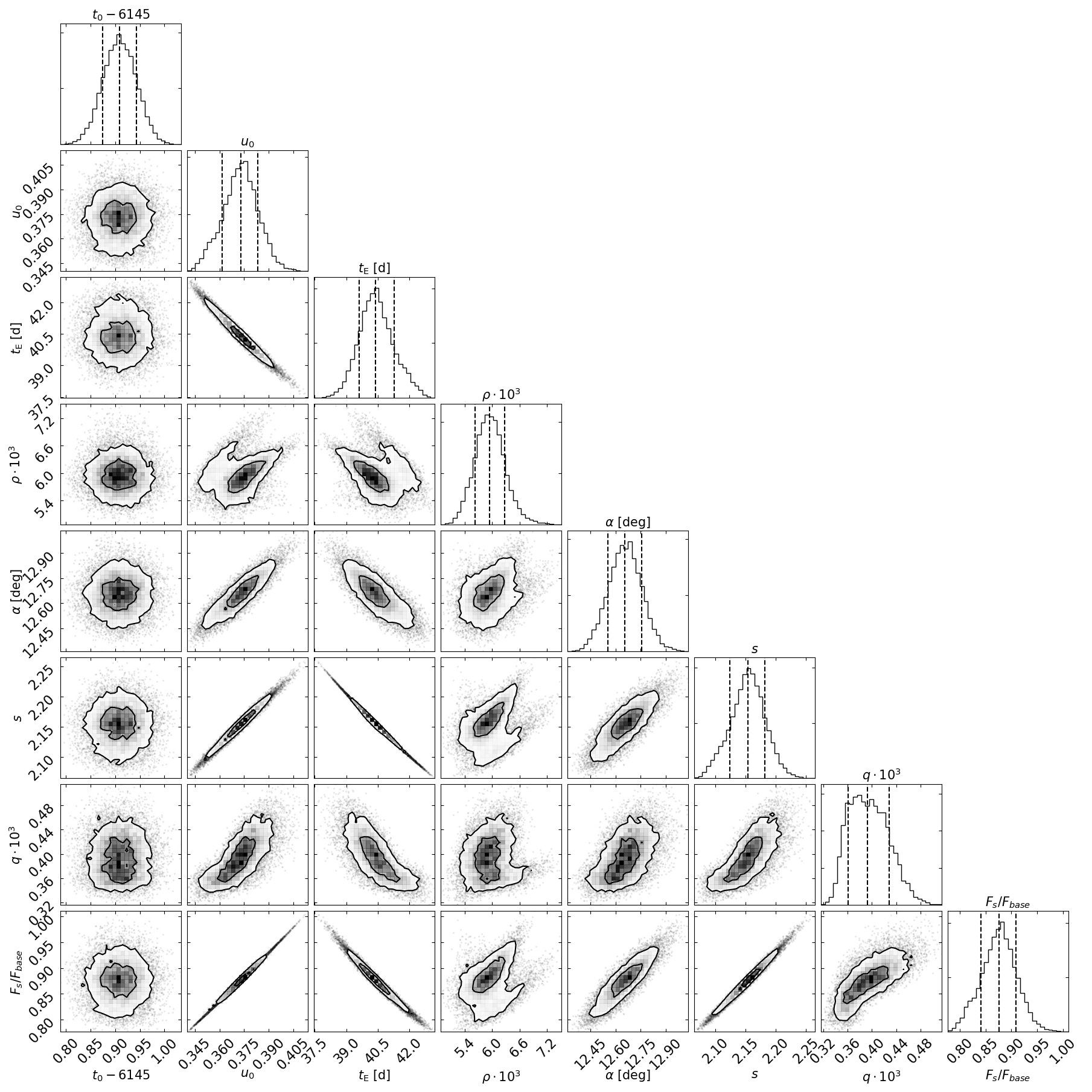
To represent a binary-lens model, we use following parameters: $t_{0}$ – the epoch of the minimum approach, $u_{0}$ – the minimum separation (normalized to $\theta_{\rm E}$), $t_{\rm E}$ – the Einstein timescale, $\rho$ – the source radius (normalized to $\theta_{\rm E}$), $\alpha$ – the angle between the source trajectory and the lens axis, $s$, and $q$. For parameter conventions we follow Skowron et al. (2011) and define $t_{0}$ and $u_{0}$ relative to the primary lens. The first three parameters ($t_{0}$, $u_{0}$, and $t_{\rm E}$) are constrained by the main subevent, i.e., their values can be obtained by fitting a point-source point-lens model to the data with the short-duration anomaly epochs removed (${\rm HJD^{\prime}}$ from 6077 to 6083). The other parameters are constrained by the time and length of the short-duration anomaly except $\rho$, and can be reasonably well estimated by visual inspection of the light curve. There are two additional flux parameters: the source flux and the blending flux. We estimate them separately for each model using linear regression. The linear limb-darkening coefficients are assumed to be $\Gamma_{I}=0.46$, $\Gamma_{MOA-R}=0.51$, and $\Gamma_{MOA,V}=0.66$, which were estimated based on a preliminary fitted model and the color-surface brightness relations by Claret & Bloemen (2011).

We explored the parameter space using the Multimodal Ellipsoidal Nested Sampling algorithm or MultiNest (Feroz & Hobson, 2008; Feroz et al., 2009). At each step MultiNest approximates the probed distribution by a union of multidimentional ellipsoids. MultiNest can sample the multimodal posterior and search for multiple separated modes, which is an important advantage. The search for multiple modes can be run on all parameters or a selected subset of parameters. Additionally, MultiNest properly calculates Bayesian evidence for each mode. In our practice, MultiNest requires more model evaluations than the Monte Carlo Markov Chain (MCMC) methods, but execution time is not a limiting factor for OGLE-2012-BLG-0838. MultiNest was able to model OGLE data alone, while MCMC methods had poor convergence.

Table 1: Wide binary-lens model for OGLE-2012-BLG-0838

Parameter	static model
$t_{0}$	$6145.909\pm 0.034$
$u_{0}$	$0.373\pm 0.011$
$t_{\rm E}$ (d)	$40.44\pm 0.84$
$\rho$	$0.00595\pm 0.00034$
$\alpha$ (deg)	$12.66\pm 0.11$
$s$	$2.153\pm 0.029$
$q$	$0.000395\pm 0.000033$
$F_{s}/F_{\rm base}$	$0.875\pm 0.035$
$\chi^{2}/{\rm d.o.f.}$	$830.72/678$

MultiNest found three separate modes whose main difference was the best-fit value of $\rho$. In particular, MultiNest found that the three modes had values of $\rho=0.0011\pm 0.0007$, $\rho=0.0037\pm 0.0002$, and $\rho=0.00595\pm 0.00034$. The first two modes require fine tuning of $u_{0}$, $t_{\rm E}$, and $s$. MultiNest not only searches for multiple modes and calculates posterior distributions of parameters, but also calculates the posterior probability of each mode. The posterior probabilities for the first and the second modes are smaller than the third one by a factor of $50$ and $180$, respectively. Additionally, the first mode predicts a large relative lens-source proper motion of $\approx 16~{}{\rm mas\,yr^{-1}}$, which is a priori unlikely. Thus, the third mode is a priori preferred and we consider only this mode as viable in the rest of the paper (details of the other two models are presented in the Appendix). We present the results of the model fitting in Table 1 and Figure 3. The best model is plotted in Figure 1.

Figure 3: Marginalized posterior constraints on the microlensing parameters of the wide binary-lens model for OGLE-2012-BLG-0838. The vertical lines in 1D histograms indicate the median and $\pm 1\sigma$ ranges.

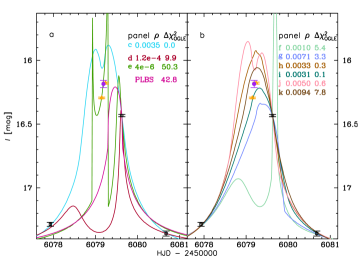
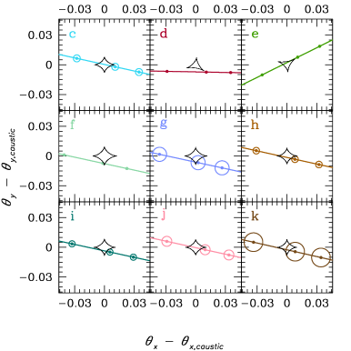
It turns out that the combination of the MOA and OGLE data restricts the number of separate modes significantly better than the OGLE data alone. When we fitted only the OGLE data and searched for multiple modes on all parameters, then MultiNest reported only a single mode. When the search for multiple modes was run only on $\rho$, then 10-30 modes were found, depending on the exact settings. The $1\sigma$ ranges of the posterior parameters of these modes were overlapping, which showed that the OGLE data alone do not allow a unique identification of multiple modes. We inspected many modes and in Figure 4 present a few modes, which were selected to show the whole range of the diversity of the light curves. The problems we faced with fitting the OGLE data alone are a less-severe case of the discrete and continuous degeneracies seen in the case of OGLE-2002-BLG-055 (Gaudi & Han, 2004), which also had only a single epoch that is much brighter than predicted by the point-source point-lens model.

Figure 4: Degenerate microlensing models for OGLE-2012-BLG-0838 fitted to OGLE data only. The upper panels (a and b) present model light curves, three OGLE epochs that constrain the anomalous part of the model (black; at $6077.9$, $6079.6$, and $6080.7$), and three MOA epochs (orange and purple; between $6079.15$ and $6079.24$). The lines shown in panel a represent best models for each of four topologies (wide: c and f-k; two close: d and e; and binary-source: pink line in panel a). The lines shown in panel b are all wide binary-lens models and were selected from the search for multiple modes run only on $\rho$. The legend gives $\rho$ and $\Delta\chi^{2}_{\rm OGLE}$ values for each model. Two models peak beyond the plot at $(6079.3,\,13.55)$ and $(6079.7,\,15.20)$. The lower panels (c-k) show the corresponding trajectories and planetary caustics (black) for the binary-lens models. The colored circles represent the size of the source as well as its position at the times when the three OGLE epochs were taken. The source is moving from left to right. The coordinate system is centered on a planetary caustic. In panels d and e, the two triangular caustics correspond to close models. In this coordinate systems, the central caustics are at $(1.56,\,-0.38)$ and $(1.57,\,0.38)$, respectively. For the other models (i.e., wide), the primary is at $(\approx 1.6,\,0)$. For the three models with $\rho<0.002$ (panels d, e, and f), the actual source size is smaller than the points shown.

We derive the source brightness using posterior distributions. We obtain $V_{s}=19.596\pm 0.044~{}{\rm mag}$, $I_{s}=17.754\pm 0.043~{}{\rm mag}$, $H_{s}=15.484\pm 0.043~{}{\rm mag}$, and $K_{s,s}=15.326\pm 0.044~{}{\rm mag}$. We also use calibrations of the MOA photometry to the OGLE-III magnitude system (Szymański et al., 2011) to derive the source brightness from the MOA data. The transformations have a scatter of $0.048~{}{\rm mag}$ in the $V$ band and $0.045~{}{\rm mag}$ in the $I$ band. We obtain $V^{\rm MOA}_{s}=19.587\pm 0.043~{}{\rm mag}$ and $I^{\rm MOA}_{s}=17.662\pm 0.043~{}{\rm mag}$, which are consistent with $V_{s}$ and $I_{s}$ derived from the OGLE data within uncertainties.

After considering the static binary-lens model, we attempted to include the microlensing parallax effect. Microlensing parallax is described by a 2D vector $\boldsymbol{\pi_{\rm E}}$, whose amplitude is equal to the relative lens-source parallax divided by $\theta_{\rm E}$. If both $\theta_{\rm E}$ and $\boldsymbol{\pi_{\rm E}}$ are measured, then both the lens mass ($M$) and distance ($D_{l}$) are measured directly (Gould, 2000):

$$M=\frac{\theta_{\rm E}}{\kappa\pi_{\rm E}},~{}~{}~{}~{}~{}~{}\frac{1}{D_{l}}=\frac{\pi_{\rm E}\theta_{\rm E}}{\rm AU}+\frac{1}{D_{s}},$$ (1)

where $\kappa=4{\rm G}/({\rm AU}\,{\rm c}^{2})=8.14~{}{\rm mas~{}M_{\odot}^{-1}}$ is a constant, and $D_{s}$ is the source distance. The annual microlensing parallax breaks the assumption that the apparent lens-source relative motion is rectilinear. The effect is undetectable for most events, because during their (typically short) duration, Earth’s motion around the Sun can be well approximated by a straight line. OGLE-2012-BLG-0838 has relatively long $t_{\rm E}$ of $40$ days. The anomaly additionally increases the chances of measuring $\pi_{\rm E}$, because it provides a well-timed event (An & Gould, 2001).

We consider two degenerate scenarios: $u_{0}<0$ and $u_{0}>0$. The best-fitting parallax model improves $\chi^{2}$ by $23.4$ and the uncertainty of $\pi_{{\rm E},N}$ is large ($\sigma_{\pi_{{\rm E},N}}=0.33$). We checked a plot of $\chi^{2}$ difference between the best parallax model and the best static model. It revealed that there may be a problem with the quality of the MOA data on a timescale of dozens of days. It is known that low-level systematics may mimic the microlensing parallax signal. Some trends in residuals of static binary-lens model can be seen in Figure 1, e.g., around ${\rm HJD^{\prime}}=6100$. Thus, we decided to report only well-established static model and do not present potentially spurious parallax models.

3.2 Close binary-lens model

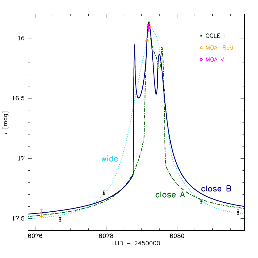
We additionally searched for close (i.e., $s<1$) binary-lens models. and found two such solutions. The parameters of these models are presented in the Appendix. The first model (marked “close A” in Figure 5) has $\chi^{2}=857.84$, i.e., it is worse fit to the data by $\Delta\chi^{2}=27.12$. The wide model is favored over the close model a priori. First, the wide model predicts the relative lens-source proper motion of $\approx 3~{}{\rm mas\,yr^{-1}}$ (see below), which is the typical value, while the close model predicts much less likely $\approx 15~{}{\rm mas\,yr^{-1}}$. Second, a recent statistical analysis of microlensing events (Suzuki et al., 2016) shows that the microlensing planet occurrence rate is increasing with increasing $s$ and decreasing $q$, and this result is confirmed by a joint analysis of microlensing, radial velocity, and direct imaging results (Clanton & Gaudi, 2016). We reject the close model based on $\Delta\chi^{2}$, as well as the two arguments given above.

The close model with $\alpha=177~{}{\rm deg}$ has a source trajectory that crosses the binary axis outside the caustics (in other words, the source passes all caustics on the same side). There is a second model in which the source trajectory crosses the binary axis between the planetary and central caustics (see the lower part of Figure 3 in Poleski et al., 2018). For OGLE-2012-BLG-0838, the latter model has $\alpha=207.20\pm 0.98~{}{\rm deg}$ (marked “close B” in Figure 5) and a corresponding $\chi^{2}$ is $876.34$, i.e., which is sufficiently larger ($\Delta\chi^{2}\simeq 45.62$) than the best fit (wide model) $\chi^{2}$ to be rejected. We compare all three binary-lens models for the anomaly part of the light curve in Figure 5.

Figure 5: Three binary-lens models for the anomalous part of the light curve fitted to OGLE and MOA data. There is a single wide model (turquoise dotted line; same as in Figure 1) and two close models: with $\alpha=177~{}{\rm deg}$ (marked A, dark green dotted-dashed line) and with $\alpha=207~{}{\rm deg}$ (marked B, dark blue solid line).

3.3 Binary-source model

The binary-source model introduces three additional parameters as compared to the point-source point-lens model ($t_{0,2}$, $u_{0,2}$ and flux ratio of two sources). The best binary-source model has $\chi^{2}$ of $988.98$, i.e., worse by $\Delta\chi^{2}\simeq 158$ than the wide binary-lens model (see the Appendix). Clearly, the wide binary-lens model fits the data better, and we reject the binary-source model.

4 System properties

Here we discuss a few different pieces of information about the lens and source. We are not able to directly measure the lens mass and distance, but we discuss the prospects for doing so. Thus, we derive the lens properties using Bayesian priors derived using a Galactic simulation. We also discuss the origin of the excess flux.

In Figure 2, we show the MagAO image of OGLE-2016-BLG-0838. The final calibrated $H$-band brightness of the target is ${H_{\rm target}}=15.29\pm 0.05~{}{\rm mag}$, where the uncertainty estimate combines the statistical and systematic components. $H_{\rm target}$ is brighter than the $H$-band source flux measured using SMARTS photometry and the difference corresponds to $H_{\rm excess}=17.26^{+0.46}_{-0.33}~{}{\rm mag}$. Later in this section we discuss where this excess flux comes from.

The relative lens-source proper motion is: $\mu_{\rm rel}=\theta_{\rm E}/t_{\rm E}=3~{}{\rm mas\,yr^{-1}}$ (see below). We may expect that the lens and source could be resolved in about ten years from now allowing the lens flux to be measured and leading to an estimate of the lens mass and distance, when combined with the stellar isochrones (Yee, 2015) and the constraint on the angular Einstein ring radius from the detection of finite source effects. In some cases, an identification of the lens in the follow-up high-resolution imaging is problematic (Bhattacharya et al., 2017). The future lens flux measurement can definitely use the MagAO image presented here for calibration. We also list nearby stars in Table 2. As one can see in Figure 2, the event is by far the brightest object within the ground-based seeing limit.

Table 2: Stars detected close to the target on MagAO image

No.	distance	$\Delta\alpha\cos\delta$	$\Delta\delta$	$H~{}{\rm[mag]}$
	[arcsec]	[arcsec]	[arcsec]
1	$0.39$	$-0.379$	$-0.026$	$17.474\pm 0.060$
2	$0.64$	$0.644$	$0.003$	$18.073\pm 0.084$
3	$0.87$	$0.742$	$-0.449$	$18.174\pm 0.070$
4	$1.02$	$-0.884$	$-0.501$	$18.469\pm 0.073$
5	$1.24$	$-1.056$	$0.652$	$16.307\pm 0.053$

Note. — $\Delta\alpha\cos\delta$ and $\Delta\delta$ indicate the displacement from the target along R.A. and Dec. directions (i.e., E and N have positive values), respectively.

Figure 6: Representative magnification curves predicted for EPOXI. The models are consistent with the OGLE data and show a range of possible magnification curves.

Figure 7: Histogram of the predicted magnification amplitude for EPOXI. The $\Delta A_{\rm EPOXI}$ values larger than $10$ are not excluded but have very low probability.

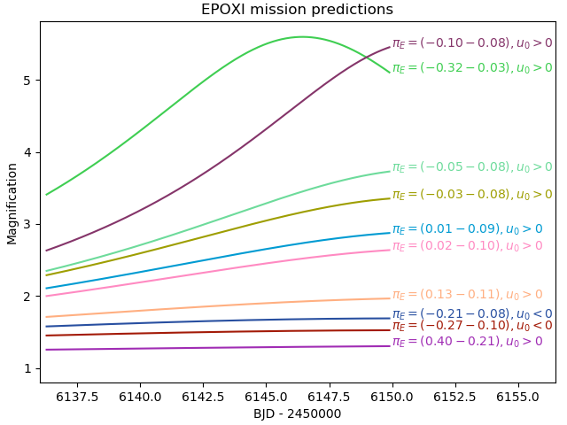
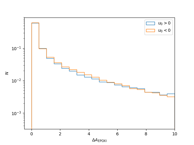
The existing EPOXI data have not yet been reduced. We use representative parallax wide binary-lens models (all are witihin $2\sigma$) fitted to the OGLE data to predict the magnification as seen by EPOXI — see Figure 6. We also show a histogram of the amplitude (i.e., difference between maximum and minimum) of magnification predicted for EPOXI in Figure 7. The lens mass and distance can be measured directly if the microlensing parallax is measured. Some of the magnification curves are almost flat. If the true magnification curve is almost flat, then the parallax measurement is unlikely. If the highest magnification is $\lesssim 4$, then the magnification curve can be reasonably well approximated as a linear function of time. In this case, it will be necessary to remove potential systematic linear trends in the EPOXI photometry in a manner that is independent of the photometry of the source in the EPOXI data in order to measure $\boldsymbol{\pi_{\rm E}}$.

Figure 8: Color–magnitude diagram for stars within $2\arcmin$ around the target. The cross marks the source position as derived from the posterior distribution. The red circle indicates the red clump (uncertainty not shown because it is smaller than the point size) and the purple square marks the blending light ($I_{b}=19.87\pm 0.30~{}{\rm mag}$, ${(V-I)}_{b}=1.93\pm 0.12~{}{\rm mag}$). The plotted OGLE data were presented and calibrated to standard photometric system by (Szymański et al., 2011).

The event parameters could be better constrained if the proper motion of the source was known. The baseline object is included in Gaia DR2 (Gaia Collaboration et al., 2018). The astrometric $\chi^{2}/{\rm dof}$ (keyword astrometric_gof_al) is $3.9$ while values $>3$ indicate bad fit to the data. The interpretation of the Gaia proper-motion measurement is additionally hindered by the fact that the baseline object is a blend of sources with detectable contribution from other stars (see Table 1). It is unlikely that Gaia DR2 proper motion can put useful constraints on system properties.

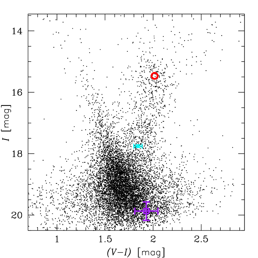
To measure $\theta_{\rm E}$, we use the method developed by Yoo et al. (2004). We present the color-magnitude diagram of stars lying within $2\arcmin$ from the target in Figure 8. The red clump has an observed color of $(V-I)_{\rm RC}=2.003\pm 0.008~{}{\rm mag}$ and a brightness of $I_{\rm RC}=15.489\pm 0.030~{}{\rm mag}$. We compare these values with the extinction-corrected values from Bensby et al. (2011) and Nataf et al. (2013), respectively, to obtain $E(V-I)=0.943~{}{\rm mag}$ and $A_{I}=1.205~{}{\rm mag}$. The extinction-corrected source properties are $I_{s,0}=16.550\pm 0.043~{}{\rm mag}$ and $V_{s,0}=17.450\pm 0.066~{}{\rm mag}$ and using the Bessell & Brett (1988) color-color relations we obtain $(V-K)_{s,0}=2.022\pm 0.147~{}{\rm mag}$. The estimated $(V-K)_{s,0}$ and $V_{s,0}$ correspond to $\theta_{\star}=1.93\pm 0.14~{}{\rm\mu as}$ (Kervella et al., 2004). When combined with $\rho$ for the wide model we obtain $\theta_{\rm E}=0.325\pm 0.029~{}{\rm mas}$.

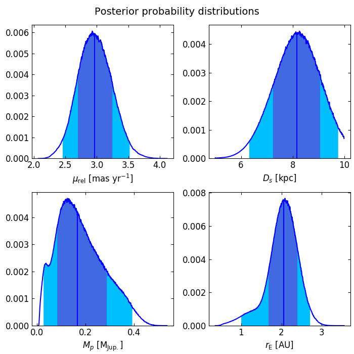
We do not have an interesting constraint on the microlensing parallax. Hence, we must use the Bayesian simulations of the Galaxy to derive the lens mass and distance. For this purpose, we use an approach similar to that presented by Clanton & Gaudi (2014). The lenses are drawn from the density profiles of a double-exponential disk (Zheng et al., 2001) and boxy Gaussian bulge (model G2 by Dwek et al., 1995), which are normalized according to Gould et al. (1996) and Han & Gould (2003), respectively. The lens mass function is taken from the model 1 in Sumi et al. (2011). For the source distance we use the boxy Gaussian bulge distribution, i.e., model G2 by Dwek et al. (1995) and weight it by $D_{s}^{2}$. The kinematics of the disk and bulge follow Clanton & Gaudi (2014). The event rate $\Gamma$ is weighted according to (Clanton & Gaudi, 2014):

$$\frac{d^{4}\Gamma}{dD_{l}dM_{l}d^{2}\boldsymbol{\mu_{\rm rel}}}=2r_{\rm E}\mu_{\rm rel}D_{l}\nu\frac{d^{2}\Gamma}{d^{2}\boldsymbol{\mu_{\rm rel}}}\frac{d\Gamma}{dM_{l}},$$ (2)

Where $r_{\rm E}=D_{l}\theta_{\rm E}$ is the Einstein ring radius projected on the lens plane and $\nu$ is the position-dependent density of lenses. A total of $1.5\cdot 10^{9}$ events were drawn. The results of the simulations are presented in Table 3 and in Figure 9.

Table 3: Posterior Physical Parameters Statistics

Parameter	unit	value
$\theta_{E}$	mas	$0.325\pm 0.029$
$\mu_{\rm rel}$	${\rm mas\,yr^{-1}}$	$2.96\pm 0.27$
$D_{s}$	kpc	$8.17\pm 0.91$
$D_{l}$	kpc	$6.32_{-1.04}^{+0.83}$
$M_{l}$	${\rm M_{\odot}}$	$0.40_{-0.20}^{+0.29}$
$M_{p}$	${\rm M_{Jup.}}$	$0.167_{-0.83}^{+0.121}$
$r_{\rm E}$	AU	$2.06_{-0.38}^{+0.33}$
$r_{\perp}$	AU	$4.43_{-0.81}^{+0.71}$

Figure 9: Posterior probability distributions from the Bayesian simulations of the Galaxy. Vertical lines indicate median values. Shade regions mark $\pm 1\sigma$ and $\pm 2\sigma$ ranges. Posteriors for lens mass and distance are plotted in Figure 11.

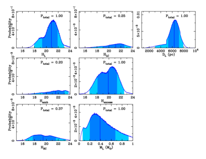
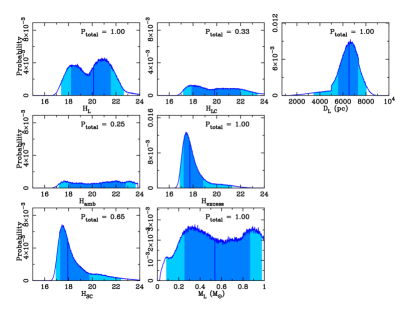
There are four possible sources contributing to the measured excess flux: the lens, unrelated ambient star(s), a companion to the source star, and a companion to the lens star. Following the method developed by Koshimoto et al. (2017) and fully described by Koshimoto et al. (2019), we calculate the probabilities of all possible combinations of the four sources that explain the observed excess flux, assuming that none of them is a stellar remnant. We use posterior distributions of $D_{s}$, $D_{l}$, and $M_{l}$ from the above Bayesian simulations as a prior to analyze the origin of the excess flux. We use the luminosity function from Zoccali et al. (2003) which is normalized to the stellar density in the OGLE-2012-BLG-0838 field to calculate the ambient stars flux distribution, where the normalization is done by comparing the number of the red clump stars in this field to that in the Zoccali et al. (2003) field using the OGLE-III catalog (Szymański et al., 2011). For the flux distribution of a companion to the source or the lens star, we use the binary distribution, which is based on Ward-Duong et al. (2015) and on the summary in a review paper of stellar multiplicity by Duchêne & Kraus (2013). We consider only companions to the source or lens whose mass ratio and semimajor axis are consistent with both the light curve and the MagAO image where no signal of a detectable stellar companion is shown. The prior distributions of parameters ($M_{l}$, $D_{l}$, and $H$-band magnitudes) are shown in Figure 11.

After deriving the prior distributions, we apply an $H_{\rm excess}$ constrained as detailed by Koshimoto et al. (2019). We present the resulting posterior distributions in Figure 11. The measured $H_{\rm excess}$ is brighter than in prior (see center panel in Figure 11), hence, adding an $H_{\rm excess}$ constraint increases the estimate of the lens mass (from $0.40_{-0.20}^{+0.29}~{}{\rm M_{\odot}}$ to $0.54_{-0.29}^{+0.33}~{}{\rm M_{\odot}}$). Also the posterior probabilities that the lens companion, the source companion, or the ambient star contribute to $H_{\rm excess}$ are higher than the corresponding prior probabilities. In particular, the probability that the source companion contributes to $H_{\rm excess}$ increased from $0.37$ to $0.65$. The main origin of $H_{\rm excess}$ is therefore more likely to be the lens or the source companion.

Figure 10: Prior probability distributions (i.e., before applying excess flux constraint). The dark vertical lines indicate median values and shaded regions mark $\pm 1\sigma$ and $\pm 2\sigma$ ranges. Each panel gives the probability that given object exists. Subscripts SC, amb, and LC stand for source companion, ambient star, and lens companion, respectively.

Figure 11: Posterior probability distributions after the $H$-band excess flux constraint is applied to prior distributions presented in Figure 11.

We can estimate the expected RV signal from OGLE-2012-BLG-0838Lb. We assume the median values for stellar host scenario from Table 3, i.e., $M_{l}=0.40~{}{\rm M_{\odot}}$ and $r_{\perp}=4.43~{}{\rm AU}$. We estimate the semi-major axis assuming a random position of the planet and a circular orbit, $a=(3/2)^{1/2}r_{\perp}=5.4~{}{\rm AU}$. The orbital period is $P=(a^{3}/M)^{1/2}=19.9~{}{\rm yr}$. For the edge-on configuration, the RV signal would be $K=3.2~{}{\rm m\,s^{-1}}$. Detecting planets with similar properties around nearby stars would be challenging for the RV surveys. The longest-period RV planets with well-measured RV curves are HR 5183b ($P\approx 74~{}{\rm yr}$ and $K=38.3~{}{\rm m\,s^{-1}}$; Blunt et al., 2019), HD 30177c ($P=20.8~{}{\rm yr}$ and $K=35.8~{}{\rm m\,s^{-1}}$ or $P=31.8~{}{\rm yr}$ and $K=59.4~{}{\rm m\,s^{-1}}$; Wittenmyer et al., 2017) and GJ 676Ac ($P=20.4~{}{\rm yr}$, $K=90.0~{}{\rm m\,s^{-1}}$; Sahlmann et al., 2016), though for neither of them the RV data cover the full orbital period. The amplitudes of the RV signals for these three planets are more than an order of magnitude larger than predicted for OGLE-2012-BLG-0838Lb.

5 Summary

We have presented the microlensing discovery of a wide-orbit planet OGLE-2012-BLG-0838Lb. Alternative models of observed light curve were considered and found inadequate. Finding planets on similar orbits around local low-mass stars presents a challenge. The lens physical properties are constrained but not directly measured. We have discussed additional existing and future data that can measure the physical parameters of the lens system directly.

Appendix A Rejected models

Tables 4, 5, and 6 present parameters of rejected wide binary-lens models, close binary-lens models, and a binary-source model, respectively. Indexes 1 and 2 indicate paramters for the first and second source, respectively.

Table 4: Two rejected wide binary-lens models for OGLE-2012-BLG-0838

Parameter
$t_{0}$	$6145.909\pm 0.029$	$6145.907\pm 0.025$
$u_{0}$	$0.3585\pm 0.0017$	$0.34289\pm 0.0028$
$t_{\rm E}$ (d)	$41.53\pm 0.14$	$42.88\pm 0.26$
$\rho$	$0.00111\pm 0.00073$	$0.00372\pm 0.00020$
$\alpha$ (deg)	$12.611\pm 0.046$	$12.438\pm 0.044$
$s$	$2.1199\pm 0.0044$	$2.0764\pm 0.0076$
$q$	$0.00389\pm 0.00019$	$0.00371\pm 0.00013$
$F_{s}/F_{\rm base}$	$0.829\pm 0.013$	$0.781\pm 0.050$
$\chi^{2}/{\rm d.o.f.}$	$835.16/678$	$836.23/678$

Table 5: Close binary-lens models for OGLE-2012-BLG-0838

Parameter	close A model	close B model
$t_{0}$	$6146.197\pm 0.041$	$6145.866\pm 0.043$
$u_{0}$	$0.3869\pm 0.0092$	$0.341\pm 0.017$
$t_{\rm E}$ (d)	$39.02\pm 0.69$	$44.8\pm 1.5$
$\rho$	$0.00123\pm 0.00012$	$0.000541\pm 0.000087$
$\alpha$ (deg)	$176.68\pm 0.92$	$207.20\pm 0.98$
$s$	$0.4554\pm 0.0053$	$0.4964\pm 0.0097$
$q$	$0.0159\pm 0.0021$	$0.0120\pm 0.0016$
$F_{s}/F_{\rm base}$	$0.920\pm 0.030$	$0.768\pm 0.049$
$\chi^{2}/{\rm d.o.f.}$	$857.84/678$	$876.34/678$

Table 6: Binary-source model for OGLE-2012-BLG-0838

Parameter	value
$t_{0,1}$	$6145.943\pm 0.035$
$u_{0,1}$	$0.417\pm 0.016$
$t_{\rm E}$ (d)	$37.37\pm 0.95$
$t_{0,2}$	$6079.3968\pm 0.0071$
$u_{0,2}$	$0.00037\pm 0.00028$
$\rho_{2}$	$0.00781\pm 0.00029$
$F_{s,1}/F_{\rm base}$	$1.027\pm 0.052$
$F_{s,2}/F_{\rm base}$	$0.00875\pm 0.00026$
$\chi^{2}/{\rm d.o.f.}$	$988.98/678$

References

- Alard (2000) Alard, C. 2000, A&AS, 144, 363, doi: 10.1051/aas:2000214
- An & Gould (2001) An, J. H., & Gould, A. 2001, ApJ, 563, L111, doi: 10.1086/338657
- Astropy Collaboration et al. (2013) Astropy Collaboration, Robitaille, T. P., Tollerud, E. J., et al. 2013, A&A, 558, A33, doi: 10.1051/0004-6361/201322068
- Astropy Collaboration et al. (2018) Astropy Collaboration, Price-Whelan, A. M., Sipőcz, B. M., et al. 2018, AJ, 156, 123, doi: 10.3847/1538-3881/aabc4f
- Baron et al. (2019) Baron, F., Lafrenière, D., Artigau, É., et al. 2019, AJ, 158, 187, doi: 10.3847/1538-3881/ab4130
- Beichman et al. (2018) Beichman, C. A., Giles, H. A. C., Akeson, R., et al. 2018, AJ, 155, 158, doi: 10.3847/1538-3881/aaaeb6
- Bensby et al. (2011) Bensby, T., Adén, D., Meléndez, J., et al. 2011, A&A, 533, A134, doi: 10.1051/0004-6361/201117059
- Bertin & Arnouts (1996) Bertin, E., & Arnouts, S. 1996, A&AS, 117, 393, doi: 10.1051/aas:1996164
- Bessell & Brett (1988) Bessell, M. S., & Brett, J. M. 1988, PASP, 100, 1134, doi: 10.1086/132281
- Bhattacharya et al. (2016) Bhattacharya, A., Bennett, D. P., Bond, I. A., et al. 2016, AJ, 152, 140, doi: 10.3847/0004-6256/152/5/140
- Bhattacharya et al. (2017) Bhattacharya, A., Bennett, D. P., Anderson, J., et al. 2017, AJ, 154, 59, doi: 10.3847/1538-3881/aa7b80
- Blunt et al. (2019) Blunt, S., Endl, M., Weiss, L. M., et al. 2019, AJ, 158, 181, doi: 10.3847/1538-3881/ab3e63
- Bond et al. (2001) Bond, I. A., Abe, F., Dodd, R. J., et al. 2001, MNRAS, 327, 868, doi: 10.1046/j.1365-8711.2001.04776.x
- Bond et al. (2017) Bond, I. A., Bennett, D. P., Sumi, T., et al. 2017, MNRAS, 469, 2434, doi: 10.1093/mnras/stx1049
- Bowler (2016) Bowler, B. P. 2016, PASP, 128, 102001, doi: 10.1088/1538-3873/128/968/102001
- Calchi Novati et al. (2015) Calchi Novati, S., Gould, A., Yee, J. C., et al. 2015, ApJ, 814, 92, doi: 10.1088/0004-637X/814/2/92
- Cassan et al. (2012) Cassan, A., Kubas, D., Beaulieu, J.-P., et al. 2012, Nature, 481, 167, doi: 10.1038/nature10684
- Chauvin et al. (2004) Chauvin, G., Lagrange, A.-M., Dumas, C., et al. 2004, A&A, 425, L29, doi: 10.1051/0004-6361:200400056
- Clanton & Gaudi (2014) Clanton, C., & Gaudi, B. S. 2014, ApJ, 791, 90, doi: 10.1088/0004-637X/791/2/90
- Clanton & Gaudi (2016) —. 2016, ApJ, 819, 125, doi: 10.3847/0004-637X/819/2/125
- Claret & Bloemen (2011) Claret, A., & Bloemen, S. 2011, A&A, 529, A75, doi: 10.1051/0004-6361/201116451
- Close et al. (2012) Close, L. M., Males, J. R., Kopon, D. A., et al. 2012, in Proc. SPIE, Vol. 8447, Adaptive Optics Systems III, 84470X, doi: 10.1117/12.926545
- Coughlin et al. (2016) Coughlin, J. L., Mullally, F., Thompson, S. E., et al. 2016, ApJS, 224, 12, doi: 10.3847/0067-0049/224/1/12
- DePoy et al. (2003) DePoy, D. L., Atwood, B., Belville, S. R., et al. 2003, in Proc. SPIE, Vol. 4841, Instrument Design and Performance for Optical/Infrared Ground-based Telescopes, ed. M. Iye & A. F. M. Moorwood, 827–838, doi: 10.1117/12.459907
- Duchêne & Kraus (2013) Duchêne, G., & Kraus, A. 2013, ARA&A, 51, 269, doi: 10.1146/annurev-astro-081710-102602
- Dwek et al. (1995) Dwek, E., Arendt, R. G., Hauser, M. G., et al. 1995, ApJ, 445, 716, doi: 10.1086/175734
- Eisner & Kulkarni (2002) Eisner, J. A., & Kulkarni, S. R. 2002, ApJ, 574, 426, doi: 10.1086/340940
- Feng et al. (2019) Feng, F., Anglada-Escudé, G., Tuomi, M., et al. 2019, MNRAS, 490, 5002, doi: 10.1093/mnras/stz2912
- Feroz & Hobson (2008) Feroz, F., & Hobson, M. P. 2008, MNRAS, 384, 449, doi: 10.1111/j.1365-2966.2007.12353.x
- Feroz et al. (2009) Feroz, F., Hobson, M. P., & Bridges, M. 2009, MNRAS, 398, 1601, doi: 10.1111/j.1365-2966.2009.14548.x
- Foreman-Mackey (2016) Foreman-Mackey, D. 2016, The Journal of Open Source Software, 1, 24, doi: 10.21105/joss.00024
- Gaia Collaboration et al. (2018) Gaia Collaboration, Brown, A. G. A., Vallenari, A., et al. 2018, A&A, 616, A1, doi: 10.1051/0004-6361/201833051
- Gaudi (1998) Gaudi, B. S. 1998, ApJ, 506, 533, doi: 10.1086/306256
- Gaudi & Han (2004) Gaudi, B. S., & Han, C. 2004, ApJ, 611, 528, doi: 10.1086/421971
- Gaudi et al. (2017) Gaudi, B. S., Stassun, K. G., Collins, K. A., et al. 2017, Nature, 546, 514, doi: 10.1038/nature22392
- Gould (2000) Gould, A. 2000, ApJ, 542, 785, doi: 10.1086/317037
- Gould et al. (1996) Gould, A., Bahcall, J. N., & Flynn, C. 1996, ApJ, 465, 759, doi: 10.1086/177460
- Gould et al. (2010) Gould, A., Dong, S., Gaudi, B. S., et al. 2010, ApJ, 720, 1073, doi: 10.1088/0004-637X/720/2/1073
- Hampton et al. (2005) Hampton, D. L., Baer, J. W., Huisjen, M. A., et al. 2005, Space Sci. Rev., 117, 43, doi: 10.1007/s11214-005-3390-8
- Han & Gould (2003) Han, C., & Gould, A. 2003, ApJ, 592, 172, doi: 10.1086/375706
- Hwang et al. (2019) Hwang, K.-H., Ryu, Y.-H., Kim, H.-W., et al. 2019, AJ, 157, 23, doi: 10.3847/1538-3881/aaf16e
- Ivezić et al. (2014) Ivezić, Ž., Connolly, A., Vanderplas, J., & Gray, A. 2014, Statistics, Data Mining and Machine Learning in Astronomy (Princeton University Press)
- Izidoro et al. (2015) Izidoro, A., Morbidelli, A., Raymond, S. N., Hersant, F., & Pierens, A. 2015, A&A, 582, A99, doi: 10.1051/0004-6361/201425525
- Kane (2011) Kane, S. R. 2011, Icarus, 214, 327, doi: 10.1016/j.icarus.2011.04.023
- Kervella et al. (2004) Kervella, P., Bersier, D., Mourard, D., et al. 2004, A&A, 428, 587, doi: 10.1051/0004-6361:20041416
- Kipping et al. (2016) Kipping, D. M., Torres, G., Henze, C., et al. 2016, ApJ, 820, 112, doi: 10.3847/0004-637X/820/2/112
- Koshimoto et al. (2019) Koshimoto, N., Bennett, D. P., & Suzuki, D. 2019, arXiv e-prints, arXiv:1910.11448. https://arxiv.org/abs/1910.11448
- Koshimoto et al. (2017) Koshimoto, N., Shvartzvald, Y., Bennett, D. P., et al. 2017, AJ, 154, 3, doi: 10.3847/1538-3881/aa72e0
- Kostov et al. (2016) Kostov, V. B., Orosz, J. A., Welsh, W. F., et al. 2016, ApJ, 827, 86, doi: 10.3847/0004-637X/827/1/86
- Lambrechts et al. (2014) Lambrechts, M., Johansen, A., & Morbidelli, A. 2014, A&A, 572, A35, doi: 10.1051/0004-6361/201423814
- Males et al. (2014) Males, J. R., Close, L. M., Morzinski, K. M., et al. 2014, ApJ, 786, 32, doi: 10.1088/0004-637X/786/1/32
- Minniti et al. (2010) Minniti, D., Lucas, P. W., Emerson, J. P., et al. 2010, New A, 15, 433, doi: 10.1016/j.newast.2009.12.002
- Morzinski et al. (2014) Morzinski, K. M., Close, L. M., Males, J. R., et al. 2014, in Proc. SPIE, Vol. 9148, Adaptive Optics Systems IV, 914804, doi: 10.1117/12.2057048
- Mróz et al. (2017) Mróz, P., Udalski, A., Skowron, J., et al. 2017, Nature, 548, 183, doi: 10.1038/nature23276
- Mróz et al. (2018) Mróz, P., Ryu, Y.-H., Skowron, J., et al. 2018, AJ, 155, 121, doi: 10.3847/1538-3881/aaaae9
- Muraki et al. (2011) Muraki, Y., Han, C., Bennett, D. P., et al. 2011, ApJ, 741, 22, doi: 10.1088/0004-637X/741/1/22
- Nataf et al. (2013) Nataf, D. M., Gould, A., Fouqué, P., et al. 2013, ApJ, 769, 88, doi: 10.1088/0004-637X/769/2/88
- Nielsen et al. (2019) Nielsen, E. L., De Rosa, R. J., Macintosh, B., et al. 2019, AJ, 158, 13, doi: 10.3847/1538-3881/ab16e9
- Paczyński (1986) Paczyński, B. 1986, ApJ, 304, 1, doi: 10.1086/164140
- Perryman et al. (2014) Perryman, M., Hartman, J., Bakos, G. Á., & Lindegren, L. 2014, ApJ, 797, 14, doi: 10.1088/0004-637X/797/1/14
- Poleski et al. (2019) Poleski, R., Penny, M., Gaudi, B. S., et al. 2019, A&A, 627, A54, doi: 10.1051/0004-6361/201834544
- Poleski & Yee (2018) Poleski, R., & Yee, J. 2018. https://ascl.net/1803.006
- Poleski & Yee (2019) Poleski, R., & Yee, J. C. 2019, Astronomy and Computing, 26, 35, doi: 10.1016/j.ascom.2018.11.001
- Poleski et al. (2014) Poleski, R., Skowron, J., Udalski, A., et al. 2014, ApJ, 795, 42, doi: 10.1088/0004-637X/795/1/42
- Poleski et al. (2018) Poleski, R., Gaudi, B. S., Udalski, A., et al. 2018, AJ, 156, 104, doi: 10.3847/1538-3881/aad45e
- Pollack et al. (1996) Pollack, J. B., Hubickyj, O., Bodenheimer, P., et al. 1996, Icarus, 124, 62, doi: 10.1006/icar.1996.0190
- Press et al. (1992) Press, W. H., Teukolsky, S. A., Vetterling, W. T., & Flannery, B. P. 1992, Numerical recipes in FORTRAN. The art of scientific computing
- Quintana et al. (2014) Quintana, E. V., Barclay, T., Raymond, S. N., et al. 2014, Science, 344, 277, doi: 10.1126/science.1249403
- Sahlmann et al. (2016) Sahlmann, J., Lazorenko, P. F., Ségransan, D., et al. 2016, A&A, 595, A77, doi: 10.1051/0004-6361/201628854
- Sako et al. (2008) Sako, T., Sekiguchi, T., Sasaki, M., et al. 2008, Experimental Astronomy, 22, 51, doi: 10.1007/s10686-007-9082-5
- Schechter et al. (1993) Schechter, P. L., Mateo, M., & Saha, A. 1993, PASP, 105, 1342, doi: 10.1086/133316
- Shvartzvald et al. (2017) Shvartzvald, Y., Yee, J. C., Calchi Novati, S., et al. 2017, ApJ, 840, L3, doi: 10.3847/2041-8213/aa6d09
- Skowron et al. (2011) Skowron, J., Udalski, A., Gould, A., et al. 2011, ApJ, 738, 87, doi: 10.1088/0004-637X/738/1/87
- Skowron et al. (2016) Skowron, J., Udalski, A., Kozłowski, S., et al. 2016, Acta Astron., 66, 1. https://arxiv.org/abs/1604.01966
- Skrutskie et al. (2006) Skrutskie, M. F., Cutri, R. M., Stiening, R., et al. 2006, AJ, 131, 1163, doi: 10.1086/498708
- Snellen & Brown (2018) Snellen, I. A. G., & Brown, A. G. A. 2018, Nature Astronomy, 2, 883, doi: 10.1038/s41550-018-0561-6
- Sumi et al. (2003) Sumi, T., Abe, F., Bond, I. A., et al. 2003, ApJ, 591, 204, doi: 10.1086/375212
- Sumi et al. (2011) Sumi, T., Kamiya, K., Bennett, D. P., et al. 2011, Nature, 473, 349, doi: 10.1038/nature10092
- Suzuki et al. (2016) Suzuki, D., Bennett, D. P., Sumi, T., et al. 2016, ApJ, 833, 145, doi: 10.3847/1538-4357/833/2/145
- Szymański et al. (2011) Szymański, M. K., Udalski, A., Soszyński, I., et al. 2011, Acta Astron., 61, 83. https://arxiv.org/abs/1107.4008
- Thommes et al. (1999) Thommes, E. W., Duncan, M. J., & Levison, H. F. 1999, Nature, 402, 635, doi: 10.1038/45185
- Tsiganis et al. (2005) Tsiganis, K., Gomes, R., Morbidelli, A., & Levison, H. F. 2005, Nature, 435, 459, doi: 10.1038/nature03539
- Udalski (2003) Udalski, A. 2003, Acta Astron., 53, 291. https://arxiv.org/abs/0807.3884
- Udalski et al. (2008) Udalski, A., Szymański, M. K., Soszyński, I., & Poleski, R. 2008, Acta Astron., 58, 69. https://arxiv.org/abs/0807.3884
- Udalski et al. (2015) Udalski, A., Szymański, M. K., & Szymański, G. 2015, Acta Astron., 65, 1. https://arxiv.org/abs/1504.05966
- Udalski et al. (2018) Udalski, A., Ryu, Y.-H., Sajadian, S., et al. 2018, Acta Astron., 68, 1. https://arxiv.org/abs/1802.02582
- Venturini & Helled (2017) Venturini, J., & Helled, R. 2017, ApJ, 848, 95, doi: 10.3847/1538-4357/aa8cd0
- Ward-Duong et al. (2015) Ward-Duong, K., Patience, J., De Rosa, R. J., et al. 2015, MNRAS, 449, 2618, doi: 10.1093/mnras/stv384
- Winn et al. (2011) Winn, J. N., Matthews, J. M., Dawson, R. I., et al. 2011, ApJ, 737, L18, doi: 10.1088/2041-8205/737/1/L18
- Wittenmyer et al. (2017) Wittenmyer, R. A., Horner, J., Mengel, M. W., et al. 2017, AJ, 153, 167, doi: 10.3847/1538-3881/aa5f17
- Wolszczan & Frail (1992) Wolszczan, A., & Frail, D. A. 1992, Nature, 355, 145, doi: 10.1038/355145a0
- Woźniak (2000) Woźniak, P. R. 2000, Acta Astron., 50, 421. https://arxiv.org/abs/0807.3884
- Yee (2015) Yee, J. C. 2015, ApJ, 814, L11, doi: 10.1088/2041-8205/814/1/L11
- Yoo et al. (2004) Yoo, J., DePoy, D. L., Gal-Yam, A., et al. 2004, ApJ, 603, 139, doi: 10.1086/381241
- Zheng et al. (2001) Zheng, Z., Flynn, C., Gould, A., Bahcall, J. N., & Salim, S. 2001, ApJ, 555, 393, doi: 10.1086/321485
- Zhu et al. (2017) Zhu, W., Huang, C. X., Udalski, A., et al. 2017, PASP, 129, 104501, doi: 10.1088/1538-3873/aa7dd7
- Zoccali et al. (2003) Zoccali, M., Renzini, A., Ortolani, S., et al. 2003, A&A, 399, 931, doi: 10.1051/0004-6361:20021604