Effects of tunneling and multiphoton transitions on squeezed–state generation in bistable driven systems

Abstract

Bistability of a nonlinear resonantly–driven oscillator in the presence of external noise is analyzed using the classical Fokker–Planck equation in the quasienergy space with account for tunneling effects and by quantum master equation in quasienergy states representation. Two timescales responsible for different stages of this bistable system relaxation have been obtained. We found that the slow relaxation rate caused by fluctuation–induced transitions between different stable states can be enhanced by several orders of magnitude due to the tunneling effects. It was also revealed that tunneling between nearly degenerate quasienergy states and resonant multiphoton transitions between the genuine eigenstates of the nonlinear oscillator are just the similar effects. It was demonstrated that the quasienergy states in the bistability region corresponding to higher amplitude are squeezed. The degree of squeezing is determined by the ratio between nonlinearity and detuning, so that the uncertainty of one quadrature can be considerably smaller than the quantum limit. We found that tunneling effects can enhance the generation of output oscillator squeezed states. It was demonstrated that 1D Fokker–Planck equation is a quasiclassical limit of a quantum master equation.

I Introduction

Complex systems with two or more stable states appear in many fields of science from biology and chemistry to quantum optics and electronics Innes et al. (2013) Semenov et al. (2016) Hoang et al. (2018) Ma et al. (2018).

Ability to control and manipulate these complex systems relies on one’s knowledge of their stable states, the extent of their robustness with respect to environmental fluctuations, and on ability to make specific perturbations inducing transitions between these states.

First, one needs to understand the behavior of bistable systems interacting with the environment. Bistable systems in optics and electronics are widely used as switching elements in communications systems, basic elements of memory devices, logic gates, optical turnstiles, etc. So, the investigation of fluctuation–induced transitions between different stable states is crucial to improve the stability of optical and electronic devices and to control their switching rates.

Due to unprecedented miniaturization of optical and electronics devices quantum effects became very important for their operation Kasprzak et al. (2010) Albert et al. (2013). It is impossible to study bistability without accounting for quantum effects. Thus, it is necessary to trace the correspondence between the classical and quantum regimes of the system Kasprzak et al. (2013). In the quantum regime it is important to understand whether quantum fluctuations impose a fundamental limit on stability of optical and electronic devices.

It is well established that in many nonlinear optical and electronic interface systems there exist a set of quantum states — squeezed states — which have less uncertainty in one quadrature than a coherent state Walls (1983). Generation of squeezed states is a key for implementation of quantum information protocols and for stability enhancement of quantum optics devices Savage and Walls (1986). Bistable quantum optics systems are promising candidates to realize the squeezed states. Recently the squeezed exciton–polariton field has been observed in pillar–shaped semiconductor microcavities in the bistable regime near the critical point of the bistable curve Boulier et al. (2014).

A driven nonlinear oscillator interacting with a thermal bath is the minimal model describing fluctuation–induced transitions in bistable systems out of equilibrium. The dynamics of various microcavities coupled with nonlinear media and coherently driven by an external field including exciton–polaritons in semiconductor microresonators with external pumping can exhibit a bistable behavior and can be described by the model of a driven nonlinear oscillator. Recent experiments demonstrated that as external coherent pumping is increased the occupied exciton–polariton mode shows strong sudden jumps from one state to another. Such behavior is caused by the fluctuation–induced transitions between the stationary states. These transitions could also lead to decrease of the hysteresis area of an internal microcavity field under the S–shaped response curve with respect to the external pumping Rodriguez et al. (2017).

Another experimental realization which can be analyzed using the nonlinear oscillator model is a mesoscopic Josephson junction array resonator Muppalla et al. (2018). In such a device, the anharmonicity can be of the same order as the linewidth, and the dynamics of bistability has been experimentally measured by observing the jumps between different stable states. It was shown experimentally that the switching rate strongly depends on the pumping intensity.

In addition, the model of a driven nonlinear oscillator is applicable to highly excited molecular vibration modes in the presence of anharmonicity.

The model of a driven nonlinear oscillator has been extensively theoretically studied since 1980’s. However, fluctuation–induced transitions between two stable states were traditionally analyzed using the classical 1D Fokker–Planck equation (FPE) in quasienergy space without accounting for quantum tunneling Vogel and Risken (1988), Maslova (1986), Dmitriev and D’yakonov (1986).

The ultra–quantum limit of dispersive bistability was analyzed by Drummond and Walls Drummond and Walls (1980), where the kinetic equation for generalized Glauber function was solved analytically for the case of zero bath temperature. The same model was analyzed numerically using the technique of quantum master equation Risken et al. (1987).

Nevertheless, there has been no detailed analysis of kinetics of the nonlinear driven oscillator allowing one to trace the transition between the classical and quantum descriptions of this system. Moreover, the structure of quasienergy states of a driven quantum nonlinear oscillator and the influence of their degeneracy Dykman and Fistul (2005) on kinetics still remains a relatively unexplored area of research. In order to understand rich physical properties of bistable systems one could start by considering the minimal model of a driven nonlinear oscillator.

In present work, we derive the quasiclassical kinetic equations taking into account the tunneling effects. These equations are a quasiclassical limit of the quantum master equation for the density matrix of a quantum driven nonlinear oscillator. We show that in the quasiclassical limit, tunneling transitions reduce the threshold value of intensity of the external field responsible for switching between the most probable states of the system. We also show that tunneling between trajectories in different regions of the phase space and multi–photon resonant transitions between the states of the nonlinear oscillator are the same effects. In the quantum case, we explore the structure of eigenstates and show that the quasienergy states corresponding to the higher amplitude stable state are squeezed, and the uncertainty in one of the quadratures can be much lower than the usual quantum limit.

II Classical bistability

II.1 The basic model

We consider a model system consisting of a single oscillator mode with Kerr–like nonlinearity excited by a resonant field. Its key feature is the bistability in a certain range of external pumping intensity: the presence of two different classical stable states.

The effective Hamiltonian for such a model is Maslova (1986), Vogel and Risken (1990), Maslova et al. (2007)

$$H_{\mathrm{eff}}=-\Delta|a|^{2}+\frac{\alpha}{2}|a|^{4}-f(a+a^{*}),$$ (1)

where $a,a^{*}$ are slowly varying amplitudes of the internal oscillator field; $\Delta\equiv\Omega-\omega_{0}$ is the detuning between the external field frequency $\Omega$ and the frequency of the resonance $\omega_{0}$; $\alpha$ is the anharmonicity parameter; $f$ is the interaction strength with external field (proportional to its amplitude). Such a model can arise for various systems in the rotating–wave approximation such as microcavity with a nonlinear medium coherently driven by an external field. For example, this effective Hamiltonian can be derived for the Janes–Cunnings model after adiabatically excluding the atomic variables. It also describes the microcavity exciton–polaritons driven by an external field as well as strongly excited vibration modes of molecules in the presence of an external resonant field. Here we use the normalized field amplitude, $A\equiv a\sqrt{\alpha/\Delta}$, and a dimensionless time, $\tau=\Delta t$. The only dimensionless parameter which governs the system dynamics is $\beta\equiv\alpha f^{2}/\Delta^{3}$. In dimensionless variables the parameter $\beta$ can be treated as the rephasing rate of the nonlinear driven oscillator Borenstein and Lamb (1972). This parameter can also be identified with the Dicke cooperation parameter determining the typical rate of the intensity growth of a superradiance pulse. Note that the original Dicke model deals with collective superradiance of the system of quantum two–level emitters interacting with the cavity field. However, as it was shown in Refs. Il’inskii and Maslova (1988) and Kocharovsky et al. (2017), a superradiance pulse can also arise in a classical system of nonlinear oscillators coupled to the cavity field due to rephasing processes.

In terms of new variables the dimensionless Hamiltonian is given by $\mathcal{H}=(\alpha/\Delta^{2})H_{\mathrm{eff}}$:

$$\mathcal{H}=-|A|^{2}+\frac{1}{2}|A|^{4}+\sqrt{\beta}(A+A^{*}),$$ (2)

while the equation of motion reads

$$i\frac{\partial A}{\partial\tau}=-A+A|A|^{2}+\sqrt{\beta}.$$ (3)

The classical phase trajectories of the nonlinear oscillator in the plane $(A,A^{*})$ are the contour lines of the classical Hamiltonian function (1) [Fig. 1(a)]. Let us focus on the structure of (1) as the function of two variables, $\operatorname{Re}A$ and $\operatorname{Im}A$.

At $\beta=0$, the function has a shape of the Mexican hat potential. It is radially symmetric, and its contour lines are concentric circles. At nonzero $\beta$, $0<\beta<\beta_{\mathrm{crit}}=4/27$, the hat is deformed, as shown in Fig. 1(b). Instead of infinitely many local minima, two extrema arise: a true local minimum and a saddle point.

The stationary values of $a$ are given by the stationary solutions of Eq. (3), which defines the S–shaped response curve (Fig. 2) of the internal field amplitude to the external field.

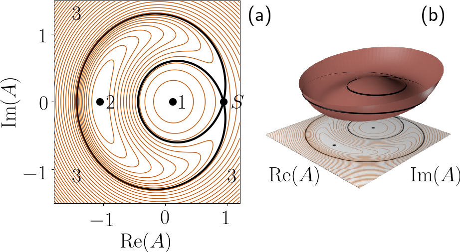
Figure 1: (a) The contour lines of the classical Hamiltonian (2) for $\sqrt{\beta/\beta_{\mathrm{crit}}}=0.3$. The separatrix (black solid line) divides the plane into three regions: region 1 containing the stationary value with a lower amplitude, region 2 containing the stationary value with a higher amplitude, and the outer region 3. The unstable stationary state S is the point of self–intersection of the separatrix. (b) The same set of contour lines is shown together with the surface plot of the Hamiltonian (2). It illustrates that the stationary states, $1$, $2$, and $S$ correspond respectively to the maximum, minimum, and the saddle point of the Hamiltonian. For each trajectory in region $1$, there exists a trajectory in region $3$ with the same quasienergy.

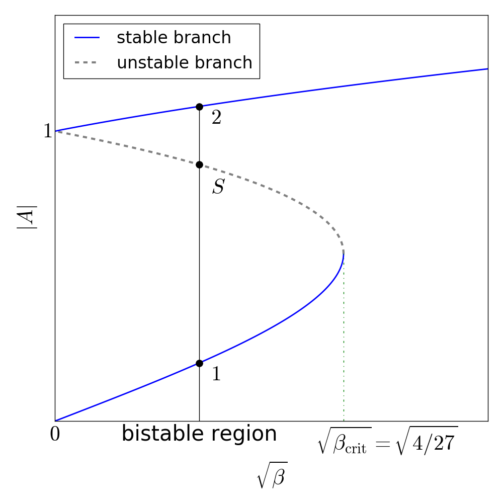
Figure 2: The S–shaped response curve of the normalized amplitude to the external field. At $\beta<\beta_{\mathrm{crit}}\equiv 4/27$ there are three stationary states. The dashed line corresponds to the unstable stationary state.

In the bistability region $0<\beta<\beta_{\mathrm{crit}}$, there are two stable stationary states 1, 2 and one unstable state S, which lies on a self–intersecting trajectory called separatrix. It divides the phase plane into three regions: the two inner regions 1 and 2 with the corresponding stable states inside them and the outer region 3. The stable state in region $1$ has a lower field amplitude, while the stable state in region $2$ has a higher field amplitude.

II.2 Fokker–Planck equation in the presence of white noise

In any realistic system, noise and damping due to interactions with the environment are always present. They result in appearance of the damping term with dimensionless damping constant $\vartheta\equiv\gamma/\Delta$ and additional random field $\xi$ in the right–hand side of the equations of motion.

$$\begin{gathered}i\frac{\partial A}{\partial\tau}=-A(1+i\vartheta)+A|A|^{2}+\sqrt{\beta}+\xi,\\ \left\langle\xi(\tau)\xi^{*}(\tau^{\prime})\right\rangle=Q\delta(\tau-\tau^{\prime}),\quad\vartheta\equiv\frac{\gamma}{\Delta}.\end{gathered}$$ (4)

The effect of damping is that the field amplitude relaxes to one of the stable stationary states. Noise has the opposite effect. First, it results in small random deviations from the stationary states. Second, it can induce transitions between the stationary states. At weak noise intensity, these transitions are exponentially rare.

In the case of the white noise (4), it is possible to derive the FPE for the probability density Johne et al. (2009).

$$\frac{\partial\mathcal{P}}{\partial t}=\frac{\partial}{\partial A}\left(i\mathcal{P}\frac{\partial H}{\partial A^{*}}+\vartheta A\mathcal{P}+\frac{Q}{2}\frac{\partial\mathcal{P}}{\partial A^{*}}\right)+\mathrm{c.c.}$$ (5)

Since the transitions between the stationary states are very rare, the relaxation consists of two stages. At first, the relaxation to the quasi–stationary distribution occurs in each region of the phase space at time scales determined by the inverse damping constant. Then, at a much slower rate, the probability distribution evolves to the true stationary distribution due to noise–induced transitions between the stable states.

At small damping ($\vartheta\ll 1$) and weak noise ($\vartheta/Q\gg 1$), a significant simplification of the 2D FPE is possible. Weak damping and noise give only a small correction to the motion along the phase trajectories. So, it is natural to average the distribution function in each region of the phase space along the trajectory and define the approximate $P_{i}(t,H(A,A^{*}))$, $i=1,2,3$.

Different trajectories with the same quasienergies can exist in regions 1 and 3 [Fig. 1]. By averaging the full FPE, one gets the 1D FPE in quasienergy space Vogel and Risken (1990), Dmitriev and D’yakonov (1986):

$$\begin{gathered}\frac{\partial P_{i}}{\partial t}=\frac{1}{T_{i}(E)}\frac{\partial J_{i}}{\partial E},\\ J_{i}(E)=\vartheta K_{i}(E)P_{i}+QD_{i}(E)\frac{\partial P_{i}}{\partial E}.\end{gathered}$$ (6)

The expressions for $K_{i}(E),D_{i}(E),T_{i}(E)$ were derived in Refs.Vogel and Risken (1990), Maslova (1986), Dmitriev and D’yakonov (1986), Maslova et al. (2007) and are reproduced in the Appendix. $T_{i}(E)$ is the period of motion along the trajectory with quasienergy $E$ in the region $i$, and $K_{i}(E)$ and $D_{i}(E)$ are the drift and the diffusion coefficients in quasienergy space in the region $i$.

This Fokker–Planck equation should be solved in every region of the phase space. The full solution should be obtained by applying the boundary conditions near the separatrix, which include the continuity of the probability distribution and the conservation of the flow:

$$\begin{gathered}P_{1}(E_{\mathrm{sep}})=P_{2}(E_{\mathrm{sep}})=P_{3}(E_{\mathrm{sep}}),\\ J_{2}(E_{\mathrm{sep}})=J_{1}(E_{\mathrm{sep}})+J_{3}(E_{\mathrm{sep}}).\end{gathered}$$ (7)

The stationary distribution can be obtained by setting the flow $J_{i}(E)$ to zero, if the tunneling effects are neglected (the discussion of the tunneling effects is given below).

II.3 Relative occupation of two stable states

The general formula for the stationary distribution function follows immediately from (6):

$$P_{i}^{\mathrm{st}}(E)=Ce^{S_{i}-S_{i}(E)},$$ (8)

$$\begin{gathered}S_{i}(E)\equiv\frac{\vartheta}{Q}\int_{E_{i}}^{E}\frac{K_{i}(E)}{D_{i}(E)}dE,\quad S_{i}\equiv S_{i}(E_{\mathrm{sep}}).\end{gathered}$$ (9)

The distribution has maxima in the vicinity of states $1$, $2$, i.e., at the corresponding quasienergies $E_{1}$, $E_{2}$ Maslova et al. (2007), Vogel and Risken (1990). Outside the neighborhood of $E_{1}$ and $E_{2}$, $P^{\mathrm{st}}_{i}(E)$ is exponentially small. Depending on whether $S_{1}>S_{2}$ or $S_{1}<S_{2}$, the probability density is mostly concentrated around either state $1$ or state $2$.

Numerical evaluation of $S_{1}$ and $S_{2}$ shows that $S_{1}=S_{2}$ at $\sqrt{\beta_{0}/\beta_{\mathrm{crit}}}=0.29$. Therefore $\beta_{0}$ corresponds to the threshold pumping intensity: at $\beta<\beta_{0}$ the oscillator mostly remains in state 1 with a small amplitude, and at $\beta>\beta_{0}$ it mostly remains in state 2 with a large amplitude. Thus the choice of the most probable state is defined by a single parameter $\beta$, and the switching from one most probable state to another occurs at the universal threshold value $\beta=\beta_{0}$. The width of the threshold region is determined by the characteristics of the noise. When $|\beta-\beta_{0}|\sim Q/\vartheta$, both states have comparable probabilities.

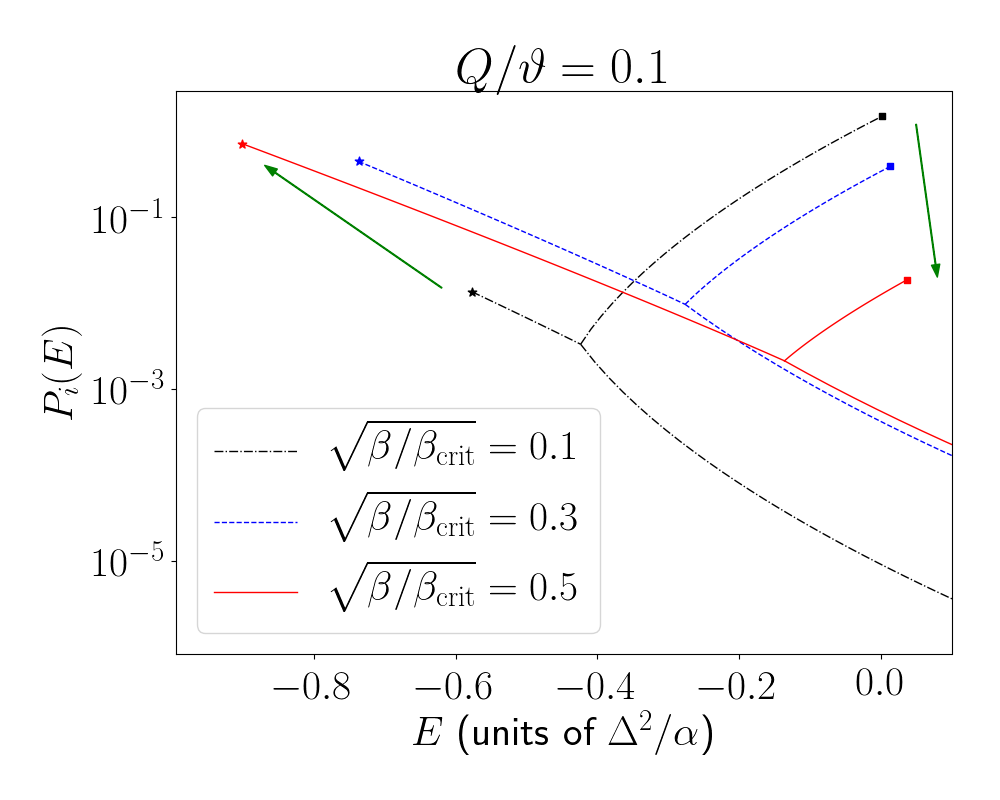
Figure 3: Stationary distribution functions of a classical nonlinear oscillator are shown for different values of $\beta$ and $Q/\vartheta=0.1$. Each distribution is single–valued at $E_{2}(\beta)<E(\beta)<E_{\mathrm{sep}}(\beta)$ and $E>E_{1}(\beta)$ and double–valued at $E_{\mathrm{sep}}(\beta)<E(\beta)<E_{1}(\beta)$, because in the latter case, there exist trajectories from regions $1$ and $3$ with the same quasienergy. The distributions have maxima at $E=E_{1,2}(\beta)$, which are shown by squares ($E_{1}$) and stars ($E_{2}$). The arrows show how the distribution function changes with increasing $\beta$. At $\beta\approx\beta_{0}$, the maxima have the same order, and at $\beta<\beta_{0}$ ($\beta>\beta_{0}$), the maximum at $E_{1}$($E_{2}$) dominates.

II.4 Transition rates between different stable states

The relaxation of a nonlinear driven oscillator happens in two stages. The first stage is the fast relaxation to the quasi–stationary distribution which occurs independently in regions $1$ and $2$. After that, the slow relaxation to the real stationary state occurs, which is governed by rare fluctuation–induced transitions between the stable states.

Every solution of the FPE can be expressed as a sum over eigenfunctions:

$$P_{i}(t,E)=\sum_{\lambda}P^{\lambda}_{i}(E)e^{-\lambda t},$$ (10)

where $\lambda$ and $P^{\lambda}$ are the solutions of the eigenvalue problem

$$-\lambda P^{\lambda}_{i}=\frac{1}{T_{i}(E)}\frac{\partial}{\partial E}\left[\vartheta K_{i}(E)+QD_{i}(E)\frac{\partial}{\partial E}\right]P^{\lambda}_{i}.$$ (11)

The eigenvalues of the FPE provide an important information about the kinetics of the system. As shown in Fig. 4, in the bistability region the lowest nonzero eigenvalue is several orders of magnitude smaller than the rest of eigenvalues. It determines the last stage of the relaxation process which was described above.

At small $Q/\vartheta$, the lowest eigenvalue $\lambda$ is exponentially small. Thus it is possible to use the perturbation theory for $P^{\lambda}_{i}$ Vogel and Risken (1990). In each region of the phase space, the distribution function up to the first order in $\lambda$ is given by

$$\begin{gathered}P^{\lambda}_{i}(E)=P^{\mathrm{st}}_{i}(E)\left[1+\frac{1}{Q}\int_{E_{\mathrm{sep}}}^{E}\frac{\Phi_{i}(E^{\prime})dE^{\prime}}{D_{i}(E^{\prime})P^{\mathrm{st}}_{i}(E^{\prime})}\right],\\ \Phi_{i}(E)=-\lambda\int_{E_{i}}^{E}dE^{\prime}T_{i}(E^{\prime})P^{\mathrm{st}}(E^{\prime}),\end{gathered}$$ (12)

where $P^{\mathrm{st}}(E)$ is the stationary distribution (8). Using the continuity of the probability distribution and the conservation of the flow, one gets the following expression for the lowest eigenvalue $\lambda$:

$$\lambda=\frac{\vartheta^{2}}{Q}\cdot\frac{K_{1}(E_{\mathrm{sep}})K_{2}(E_{\mathrm{sep}})}{K_{2}(E_{\mathrm{sep}})-K_{1}(E_{\mathrm{sep}})}\left[\frac{e^{-S_{2}}}{D_{2}^{\prime}(E_{2})}-\frac{e^{-S_{1}}}{D_{1}^{\prime}(E_{1})}\right].$$ (13)

It is clear that the analytical expression (13) fits well the numerical results everywhere in the bistability region except in the vicinity of its edges [Fig. 4].

The lowest eigenvalue non–monotonically depends on the value of $\beta$ and achieves its minimum at $\beta=\beta_{0}$. At $\beta<\beta_{0}$ ($\beta>\beta_{0}$), it corresponds to the escape rate $\lambda_{21}$ ($\lambda_{12}$) from the higher (lower) amplitude state to the lower (higher) one, which drops (rises) with the growing external field intensity. At the threshold intensity $\beta_{0}$, $\lambda_{12}$ and $\lambda_{21}$ have the same values.

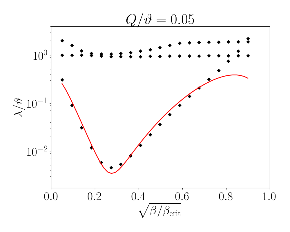
Figure 4: The exact nonzero eigenvalues of the FPE at $Q/\vartheta=0.05$ (black diamonds) are compared with the asymptotic formula (13) (red line). The lowest nonzero eigenvalue is well below $\gamma$ and all other eigenvalues, which have the order of $\gamma$. The asymptotic formula fits well the true lowest eigenvalue when it is smaller than $\vartheta$, and is not too close to the edges of the bistability region.

II.5 A tunneling term in the Fokker–Planck equation

The trajectories in regions $1$ and $3$ can have the same quasienergy. Thus there is a possibility of quantum tunneling between them. In the quasiclassical language, it can be described as the tunneling term in the FPE:

$$\begin{gathered}\frac{\partial P_{(1,3)}}{\partial t}=\frac{1}{T(E)}\frac{\partial J_{(1,3)}}{\partial E}+\lambda_{T}(E)(P_{(3,1)}-P_{(1,3)}).\\ \end{gathered}$$ (14)

Here, $\lambda_{T}$ is the tunneling rate. It can be calculated in the quasiclassical limit with the tunneling amplitude proportional to $e^{-\frac{\Delta}{\hbar\alpha}S_{\mathrm{tunn}}(E)}$ using the Fermi’s golden rule:

$$\lambda_{T}/\vartheta\sim e^{-\frac{2\Delta}{\hbar\alpha}S_{\mathrm{tunn}}(E)}.$$ (15)

At small $\lambda_{T}$, the stationary solution $P^{T}_{i}(E)$ can be obtained by the perturbation approach similar to (12):

$$\begin{gathered}P^{T}_{(1,3)}(E)=P^{\mathrm{st}}_{(1,3)}(E)\left[1+\frac{1}{Q}\int_{E_{\mathrm{sep}}}^{E}\frac{\tilde{\Phi}_{(1,3)}(E^{\prime})dE^{\prime}}{D(E^{\prime})P^{\mathrm{st}}_{(1,3)}}\right],\\ \tilde{\Phi}_{(1,3)}(E^{\prime})=\int_{E_{(1,\mathrm{sep})}}^{E^{\prime}}dE^{\prime\prime}T(E^{\prime\prime})\lambda_{T}(E^{\prime\prime})(P_{(1,3)}^{\mathrm{st}}-P_{(3,1)}^{\mathrm{st}}).\end{gathered}$$ (16)

From this equation, we can determine the most probable quasienergy states in regions 1 and 3 from which the tunneling occurs. It is defined by the minimum of $S_{\mathrm{total}}$,

$$S_{\mathrm{total}}=\frac{2\Delta}{\hbar\alpha}S_{\mathrm{tunn}}(E)+\frac{\vartheta}{Q}S_{i}(E).$$ (17)

For calculation of the quasiclassical tunneling exponent $S_{\mathrm{tunn}}$ it is necessary to rewrite the classical Hamiltonian (1) in real variables $p$ and $q$: $A=\frac{q+ip}{\sqrt{2}}$:

$$\mathcal{H}=-\left(\frac{q^{2}+p^{2}}{2}\right)+\frac{1}{2}\left(\frac{q^{2}+p^{2}}{2}\right)^{2}-\sqrt{2\beta}q.$$ (18)

The tunneling action is defined as an integral over the classically inaccessible area $p^{2}<0$:

$$S_{\mathrm{tunn}}=\int_{q_{1}}^{q_{c}}|p_{1}|dq+\int_{q_{c}}^{q_{2}}|p_{3}|dq.$$ (19)

The functions $p_{1,3}(q)$ for a specific quasienergy $E$ are determined as the solutions of the equation $\mathcal{H}(p,q)=E$:

$$p^{2}_{1,3}=2-q^{2}\pm 2\sqrt{1+2E-2\sqrt{2\beta}q}.$$ (20)

The turning points $q_{1}$, $q_{2},q_{c}$ are defined by the conditions $p_{1}^{2}(q_{1})=0$, $p_{3}^{2}(q_{2})=0$, and $p_{1}^{2}(q_{c})=p_{3}^{2}(q_{c})$.

The resulting quasiclassical tunneling exponent has an integral representation

$$S_{\mathrm{tunn}}=\int_{q_{1}}^{q_{2}}\operatorname{acosh}\left\{\frac{E+\frac{x^{2}}{2}-\frac{x^{4}}{8}}{\sqrt{2\beta}x}\right\}x\,dx.$$ (21)

At small $\beta/\beta_{\mathrm{crit}}$, it can be approximated as

$$S_{\mathrm{tunn}}=\sqrt{1+2E}\ln{\frac{1}{\beta}}+O(1).$$ (22)

Now, from the expression (17) we can estimate the quasienergy state which is optimal for tunneling.

At $\vartheta/Q\gg\Delta/\hbar\alpha$, $S_{\mathrm{total}}$ has a minimum near $E\sim E_{1}$, Therefore tunneling transitions occurs directly between the lower–amplitude stable state and the corresponding state from region 3. On the contrary, at $\vartheta/Q\ll\Delta/\hbar\alpha$ the ”total action” $S_{\mathrm{total}}$ has a minimum near $E\sim E_{\mathrm{sep}}$. So, tunneling occurs between the states with quasienergy close to $E_{\mathrm{sep}}$, and the noise–induced transitions dominate.

We concentrate on the case $\vartheta/Q\gg\Delta/\hbar\alpha$. In this limit, the leading term in the tunneling action at $E=E_{1}$ is

$$S_{\mathrm{tunn}}(E_{1})=\ln{\frac{1}{\beta}}+O(1).$$ (23)

The pre–exponential factor has the order of $\Delta$. It can be evaluated by matching the quasiclassical solutions near the turning points.

Tunneling between the quasiclassical trajectories effectively occurs when the quasienergies obtained from the Bohr–Sommerfeld quantization rule become almost equal. In this case, tunneling leads to an exponentially small splitting between them. As will be shown below, even at finite $\beta$, this occurs when $2\Delta/\hbar\alpha$ is exactly integer. In this case, the tunneling rate between the classical trajectories in regions 1 and 3 with closest quasienergies is estimated as

$$\lambda_{T}\propto\frac{\Delta^{2}}{\gamma}\beta^{\frac{2\Delta}{\hbar\alpha}}.$$ (24)

When $2\Delta/\hbar\alpha$ is not integer, and $\gamma\ll\Delta$, one has

$$\lambda_{T}\propto\gamma\beta^{\frac{2\Delta}{\hbar\alpha}}.$$ (25)

In both cases, the tunneling rate is proportional to $\beta^{\frac{2\Delta}{\hbar\alpha}}$. At integer $2\Delta/\hbar\alpha=m$, the tunneling rate can be treated as the probability of $m$–photon resonant transition between the real energy states of the nonlinear oscillator. So, the tunneling processes in the presence of a resonant external field and the multi–photon transitions between the energy states of a nonlinear oscillator are the similar effects Keldysh (1965).

The same expression for the tunneling amplitude in the lowest non–vanishing order can be also obtained in the framework of the quantum–mechanical perturbation theory for multi–photon transitions Larsen and Bloembergen (1976):

$$A_{k,m-k}=\frac{\Delta}{m}\left(\frac{\beta m^{3}}{2}\right)^{\frac{m}{2}-k}\frac{\sqrt{(m-k)!}}{(m-2k-1)!^{2}\sqrt{k!}}.$$ (26)

For $k=0$,

$$|A_{0,m}|^{2}\propto\Delta^{2}\beta^{m}.$$ (27)

The state with $k=0$ corresponds to the point 1 on the phase portrait. So, for a driven bistable system, the probability of $m$–photon transition calculated quantum–mechanically (26) is the same as the tunneling probability between the degenerate quasienergy states in the quasiclassical treatment.

The same nature of tunneling effects and multi–photon ionization of atoms in a strong electromagnetic field was first demonstrated by L. V. Keldysh Keldysh (1965).

The presence of tunneling modifies both the distribution function and the relaxation rate. If $\lambda_{T}$ is small, its effect can be taken into account within the perturbation theory. The ratio of probability densities of states $1$, $2$ modifies as follows:

$$\frac{P_{2}^{\mathrm{st}}(E_{2})}{P_{1}^{\mathrm{st}}(E_{1})}=e^{S_{2}}\left(e^{-S_{1}}+\frac{\lambda_{T}(E_{1})Q}{\vartheta^{2}}\frac{D^{\prime}_{1}(E_{1})}{K_{1}(E_{\mathrm{sep}})}\right).$$ (28)

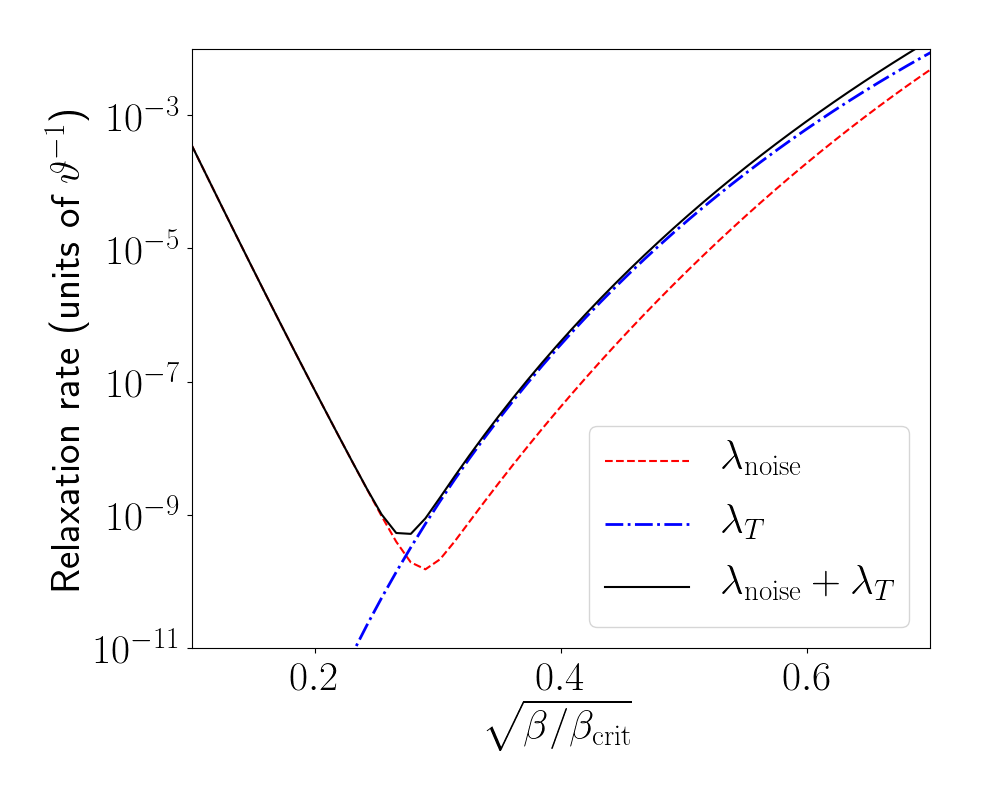
Figure 5: The relaxation rate in units of $\vartheta$ without and with the tunneling term. Here $Q=0.015$ and $\hbar\alpha/\Delta=0.2$

According to this formula, tunneling leads to a decreasing probability to be in state $1$. Tunneling also changes the total transition rate between the stable states:

$$\lambda_{\mathrm{total}}=\lambda_{\mathrm{noise}}+\lambda_{T}(E_{1}).$$ (29)

Here, $\lambda_{\mathrm{noise}}$ is defined by (13).

The behavior of the transition rate between the stable states in the presence of tunneling is depicted in Fig. 5. Tunneling transitions shift the threshold value of the external field intensity towards lower values and increase the threshold values of the transition rate.

III Bistability in quantum oscillator

III.1 Quantum quasienergy states and squeezing

The Hamiltonian for a quantum bistable oscillator in the rotating–wave approximation is given by:

$$\begin{gathered}\hat{H}_{0}=-\Delta\hat{a}^{\dagger}\hat{a}+\frac{\alpha}{2}\hat{a}^{\dagger}\hat{a}^{\dagger}\hat{a}\hat{a}+f(\hat{a}+\hat{a}^{\dagger}),\\ [\hat{a},\hat{a}^{\dagger}]=1.\end{gathered}$$ (30)

The operators $\hat{a}$ and $\hat{a}^{\dagger}$ are the creation and annihilation operators of the internal oscillator field. In the quasiclassical limit, $\sqrt{\hbar}\hat{a}$ and $\sqrt{\hbar}\hat{a}^{\dagger}$ correspond to the classical field amplitudes. In the following, we set $\hbar=1$.

The exact eigenstates of (30) should be obtained numerically by diagonalization of the Hamiltonian matrix. However, qualitatively, the structure of eigenstates can be understood using the classical analogy.

From the Bohr–Sommerfeld quantization rule, one concludes that the eigenstates of the Hamiltonian correspond to the discrete set of trajectories in the classical phase portrait (Fig. 1). However, the real picture is a bit more complicated because the quantum tunneling should also be taken into account. This is because the classical phase portrait has different regions with the same quasienergy, i.e., regions I and III. So, the real eigenstates may correspond not only to single trajectories but also to superpositions of two trajectories with the same quasienergy.

The possibility of quantum tunneling is closely connected to the degeneracy of eigenstates in the Hamiltonian (30) at $f=0$. At $f=0$, the Hamiltonian commutes with $a^{\dagger}a$, and the states with $k$ excitation quanta are the eigenstates of the Hamiltonian. Their quasienergy is

$$\epsilon_{k}^{(0)}=-\Delta k+\frac{\alpha k(k-1)}{2}.$$ (31)

For integer $2\Delta/\alpha$, the states with $k$ and $m-k$ excitation quanta become degenerate. At small but nonzero $f$, these states can mix: the true eigenstates are the superpositions of $|k\rangle$ and $|m-k\rangle$. In the quasiclassical language, this corresponds to tunneling between degenerate classical trajectories. Numerical diagonalization shows that such mixing occurs only when $2\Delta/\alpha$ is very close to an integer.

To provide some illustration to this qualitative picture, we calculated the eigenstates of the Hamiltonian (30) in the coherent basis:

$$\psi_{n}(z)\equiv\langle n|z\rangle,$$ (32)

where $|z\rangle$ is a normalized coherent state. The function $\psi_{n}(z)$ corresponding to the $n$–th eigenstate has a maximum near the contour line of the classical Hamiltonian $H(a,a^{*})=E_{n}$. This means that the quantum state $|n\rangle$ corresponds to the classical motion along the trajectory $H(a,a^{*})=E_{n}$.

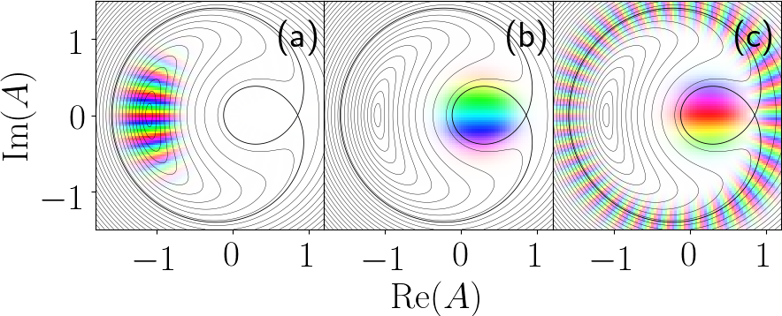
Figure 6: Some eigenstates of the quantum Hamiltonian are shown in the coherent basis. For each state $|n\rangle$, we show the quantity $\langle z|n\rangle$ in complex $z$ plane ($z=A\sqrt{\Delta/\alpha}$). (a) The higher–amplitude state for $\Delta/\alpha=20.25$ and $\sqrt{\beta/\beta_{\mathrm{crit}}}=0.6$. It is squeezed in the $q$–direction. (b) The lower–amplitude state for the same parameters. (c) The eigenstate which is a superposition of the lower–amplitude state and the trajectory from the classical region $3$. It corresponds to $\Delta/\alpha=20$ and $\sqrt{\beta/\beta_{\mathrm{crit}}}=0.6$.

An important property of the quasienergy states is that the states corresponding to the higher amplitude stable point are squeezed. This can be shown by the mean–field expansion:

$$\begin{gathered}\hat{a}=\left\langle a\right\rangle_{2}+\hat{a}^{\prime}.\\ \end{gathered}$$ (33)

The mean value of $\hat{a}$ is defined from the equation $\frac{\partial H}{\partial a}(\left\langle a\right\rangle_{2},\left\langle a^{*}\right\rangle_{2})=0$, which corresponds to the classical stable states $i$. For small $\beta$, the mean field value in the higher amplitude stable state 2 is $\langle a\rangle_{2}\approx\sqrt{\Delta/\alpha}(1+\sqrt{\beta}/2)$.

The quadratic part of the Hamiltonian takes the form

$$\hat{H}=H(\left\langle a\right\rangle_{2},\left\langle a^{*}\right\rangle_{2})-(\Delta-2\alpha|\langle a\rangle_{2}|^{2})\hat{a}^{\prime\dagger}\hat{a}^{\prime}\\ +\frac{\alpha}{2}\langle a\rangle_{2}^{2}\hat{a}^{\prime\dagger}\hat{a}^{\prime\dagger}+\frac{\alpha}{2}\langle a^{\dagger}\rangle_{2}^{2}\hat{a}^{\prime}\hat{a}^{\prime}.$$ (34)

We diagonalize this Hamiltonian using the Bogolyubov transformation:

$$\begin{gathered}\hat{a}^{\prime}=\hat{b}\cosh\theta-\hat{b}^{\dagger}\sinh\theta,\\ \tanh{2\theta}=\frac{\alpha|\langle a\rangle_{2}|^{2}}{2\alpha|\langle a\rangle_{2}|^{2}-\Delta}.\end{gathered}$$ (35)

Let us consider the uncertainties in two quadratures $\hat{q}$ and $\hat{p}$, $\hat{a}=\frac{\hat{q}+i\hat{p}}{\sqrt{2}}$. Squeezing is more pronounced in the higher amplitude stable states $\langle a\rangle_{2}$.

$$\begin{gathered}\left\langle q^{2}\right\rangle-\langle q\rangle_{2}^{2}=\frac{e^{-2\theta}}{2}=\frac{1}{2}\sqrt{\frac{\alpha|\langle a\rangle_{2}|^{2}-\Delta}{3\alpha|\langle a\rangle_{2}|^{2}-\Delta}},\\ \left\langle p^{2}\right\rangle-\langle p\rangle_{2}^{2}=\frac{e^{2\theta}}{2}=\frac{1}{2}\sqrt{\frac{3\alpha|\langle a\rangle_{2}|^{2}-\Delta}{\alpha|\langle a\rangle_{2}|^{2}-\Delta}}.\end{gathered}$$ (36)

The quadratic approximation is correct when $\sqrt{\beta}$ is larger than $\alpha/\Delta$. When $\alpha/\Delta\ll 1$, this is fulfilled almost in the entire region of bistability, and the relations (36) are valid.

The minimum possible uncertainty of $\hat{q}$ is at $\beta\sim(\alpha/\Delta)^{2}$, where it can be estimated as

$$\left\langle q^{2}\right\rangle-\left\langle q\right\rangle_{2}^{2}\sim\sqrt{\frac{\alpha}{\Delta}}.$$ (37)

Thus, the uncertainty in $\hat{q}$ quadrature can be far beyond the quantum limit.

As we have shown in the previous section (28), the tunneling effects increase the occupation of the stable state 2 with a higher amplitude and therefore enhance the generation of squeezed states.

III.2 Quantum kinetic equation

Let us assume that the system is weakly interacting with the environment:

$$H_{\mathrm{full}}=H_{0}+\hat{\xi}^{\dagger}\hat{a}+\hat{\xi}\hat{a}^{\dagger}+H_{\mathrm{bath}}.$$ (38)

We assume that the correlation functions of damping operators are delta–correlated:

$$\begin{gathered}\left\langle\hat{\xi}(t)\hat{\xi}^{\dagger}(t^{\prime})\right\rangle=\gamma(N+1)\delta(t-t^{\prime}),\\ \left\langle\hat{\xi}^{\dagger}(t)\hat{\xi}(t^{\prime})\right\rangle=\gamma N\delta(t-t^{\prime}),\\ \end{gathered}$$ (39)

where $N$ is the number of noise quanta.

With such assumptions, the density matrix evolution can be described by the master equation Haken (1965), Risken (1965), Graham and Haken (1970). Drummond and Walls (1980), Risken et al. (1987):

$$\partial_{t}\rho=i[\rho,H]+\frac{\gamma}{2}(2\hat{a}\rho\hat{a}^{\dagger}-\rho\hat{a}^{\dagger}\hat{a}-\hat{a}^{\dagger}\hat{a}\rho+2N[[\hat{a},\rho],\hat{a}^{\dagger}]).$$ (40)

If $\gamma$ is small compared to $\Delta$, the density matrix is almost diagonal in the basis of eigenstates $|n\rangle$, and the master equation reduces to the rate equation for probabilities $P_{n}$ to be in the $n$–th eigenstate:

$$\begin{gathered}\frac{dP_{n}}{dt}=\sum_{n^{\prime}}w_{nn^{\prime}}P_{n^{\prime}}-w_{n^{\prime}n}P_{n},\\ w_{nn^{\prime}}=\gamma\left[(N+1)|\langle n|\hat{a}|n^{\prime}\rangle|^{2}+N|\langle n^{\prime}|\hat{a}|n\rangle|^{2}\right].\end{gathered}$$ (41)

This equation is a quantum analog of (6). The evolution of the density matrix has the same features as the evolution of the distribution function for a classical oscillator with bistability. At infinite time, the density matrix evolves to the stationary distribution. The relaxation to $P^{\mathrm{st}}_{n}$ consists of two stages. The first stage corresponds to the relaxation to the quasi–stationary distribution. Its typical time is $\gamma^{-1}$. The second stage is the relaxation to the true stationary state. This stage is very slow and happens due to transitions between the classical stationary states. These transitions can be induced by quantum fluctuations as well as by thermal noise.

Formally, the general solution of (41) reads

$$P_{n}(t)=P_{n}^{\mathrm{st}}+\sum_{\lambda>0}C_{k}P^{\lambda}_{n}e^{-\lambda t},$$ (42)

The lowest nonzero eigenvalue is much smaller than all other eigenvalues. Therefore, at large $t$ only the term with the lowest nonzero $\lambda$ should be retained in Eq. (42).

The density matrix relaxes to the true stationary distribution with the rate $\lambda_{\mathrm{min}}$, which can be interpreted as the rate of fluctuation–induced transitions between the stable states.

III.3 The quasiclassical limit

One can show that the continuous limit of (41) is the (6). As it was mentioned above, every eigenstate corresponds to a trajectory on the classical phase portrait, and the hybridization of the trajectories from regions $1$ and $3$ can be neglected unless $2\Delta/\alpha$ is very close to an integer. Thus, in the quasiclassical limit, the distribution function $P_{n}$ weakly depends on $n$ in each of the regions of the phase space. Moreover, the transition rates $w_{n,n^{\prime}}\equiv\tilde{w}_{\bar{n},k}$, $\bar{n}=\frac{n+n^{\prime}}{2}$, $k=n^{\prime}-n$ decrease fast with an increasing value of $|k|$ and weakly depend on $\bar{n}$, which is close to $n$. In this case, it is possible to perform a gradient expansion of $P_{n}$, $w_{nn^{\prime}}$ in (41):

$$P_{n+k}=P_{n}+\frac{\partial P_{n}}{\partial n}k+\frac{1}{2}\frac{\partial^{2}P_{n}}{\partial n^{2}}k^{2}+\dots,$$ (43)

$$w_{n,n+k}=\tilde{w}_{n,k}+\frac{\partial\tilde{w}_{n,k}}{\partial\bar{n}}\left(\frac{k}{2}\right)+\frac{1}{2}\frac{\partial^{2}\tilde{w}_{n,k}}{\partial\bar{n}^{2}}\left(\frac{k}{2}\right)^{2}+\dots$$ (44)

In (44), we took into account that $w_{n,n+k}=\tilde{w}_{n+\frac{k}{2},k}=\tilde{w}_{\bar{n},k}$, $\bar{n}=n+\frac{k}{2}$. Keeping the terms up to the second order in $k$, one obtains the differential equation for $P_{n}$:

$$\frac{\partial P_{n}}{\partial t}=\frac{\partial}{\partial n}\left[A(n)P_{n}+B(n)\frac{\partial P_{n}}{\partial n}\right],$$ (45)

where the coefficients $A(n)$ and $B(n)$ are given by the expressions (41) for probabilities $w_{nn^{\prime}}$:

$$A(n)=-\sum_{k}\tilde{w}_{n,k}k=\frac{i\gamma\tilde{T}(\epsilon_{n})}{2\pi}\left\langle n|\hat{a}\,\partial_{t}\hat{a}^{\dagger}|n\right\rangle,$$ (46)

$$\begin{gathered}B(n)=\frac{1}{2}\sum_{k}\tilde{w}_{n,k}k^{2}=\gamma\left(N+\frac{1}{2}\right)\frac{\tilde{T}(\epsilon_{n})^{2}}{4\pi^{2}}\left\langle n|\partial_{t}\hat{a}\partial_{t}\hat{a}^{\dagger}|n\right\rangle.\end{gathered}$$ (47)

Here $\tilde{T}(\epsilon_{n})$ is the period of the classical motion with quasienergy $\epsilon_{n}$.

In the quasiclassical limit, the averages over the quantum quasienergy states transform to time–averages over the classical trajectories. Thus, in the quasiclassical limit, $A(n)$ and $B(n)$ are expressed as line integrals over the classical trajectories:

$$\begin{gathered}A(n)=\frac{i\gamma}{4\pi}\oint_{C(\epsilon_{n})}a\,da^{*}-a^{*}da,\\ B(n)=\frac{i\gamma\tilde{T}(\epsilon_{n})}{8\pi^{2}}\left(N+\frac{1}{2}\right)\oint_{C(\epsilon_{n})}\frac{\partial H}{\partial a}da-\frac{\partial H}{\partial a^{*}}da^{*}.\\ \end{gathered}$$ (48)

After a change of variables $\frac{\Delta}{\alpha}T(E)dE=2\pi dn$, $t\Delta=\tau$, and $\gamma/\Delta=\vartheta$ the equation transforms to the classical FPE (6). The coefficient $A(n)$ transforms to $\vartheta K(E)$, and $B(n)$ transforms to $QT(E)D(E)$, where

$$Q=\frac{\vartheta\alpha}{\Delta}\left(N+\frac{1}{2}\right),$$ (49)

$E=\alpha\epsilon/\Delta^{2}$ is the dimensionless quasienergy, and $T(E)=\Delta\tilde{T}(E\Delta^{2}/\alpha)$ is the dimensionless period as in (6).

III.4 Results and discussion

Qualitatively, the behavior of $P^{\mathrm{st}}_{n}$ in the diagonal approximation resembles the behavior of $P^{\mathrm{st}}_{i}(E)$ of a classical oscillator, as $P^{\mathrm{st}}_{i}(E)$ is the classical limit of $P^{\mathrm{st}}_{n}$ (here $i$ indicates the classical region of the phase space). As $P^{\mathrm{st}}_{i}(E)$, it consists of two sharp peaks which can be attributed to the classical stable states $1$ and $2$. Below (above) the threshold value of the external field, the state $1$ ($2$) dominates.

We directly compared the distributions obtained from the classical FPE and from the quantum master equation. In the classical limit $P^{\mathrm{st}}_{n}$ equals $(2\pi\alpha/\Delta)P_{i}^{\mathrm{st}}(E_{n})$, $E_{n}=\alpha\epsilon_{n}/\Delta^{2}$, where $P^{\mathrm{st}}_{i}(E)$ is the classical distribution function for a dimensionless Hamiltonian (2) with number of noise quanta defined by (49). The index $i$ corresponding to the classical region of the phase space is uniquely defined for each eigenstate unless $2\Delta/\alpha$ is an integer. In the latter case, the classical FPE should be derived from the quantum master equation more carefully. It can be obtained only after choosing the proper basic quasienergy states. One should deal with the quantum states corresponding to the trajectories in the regions of phase space 1 and 3, but not with their superposition.

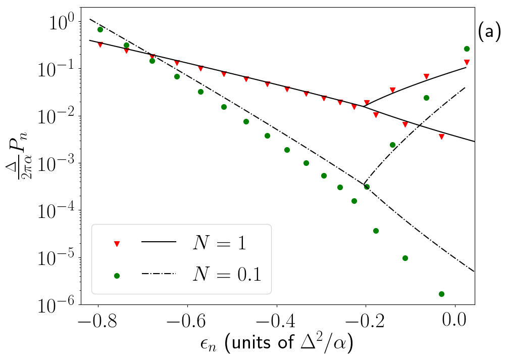
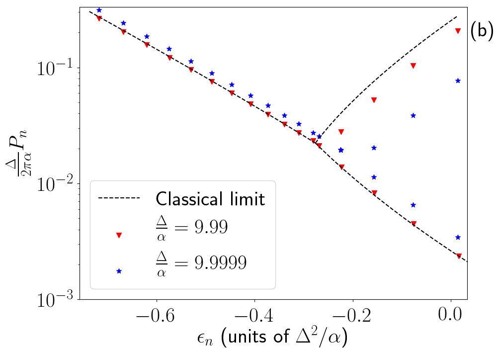
Figure 7: (a) The quantum analog of classical distribution function for $\Delta/\alpha=9.8$, $\sqrt{\beta/\beta_{\mathrm{crit}}}=0.3$ and $N=0.1,1$. Solid (dashed) line represents the classical distribution for $N=1(0.1)$, triangles (circles) represent the quantum distribution for $N=1(0.1)$. For $N=1$, the quantum distribution fits well the corresponding classical distribution. For $N=0.1$, the quantum and classical distribution differ significantly. (b) The distribution functions at $N=1$ and different closely spaced values of $\Delta/\alpha$. At $\Delta/\alpha=9.99$ (red triangles), the distribution is close to the classical distribution (black dashed line). At $\Delta/\alpha=9.9999$ (blue stars), the population in the lower–amplitude state is significantly smaller than the prediction of the classical FPE.

For the classical case, it was shown that the change of the most probable stable state takes place at $\sqrt{\beta}\equiv\sqrt{\alpha f^{2}/\Delta^{3}}\approx 0.29$. From Fig. 7, it is clear that for a rather high number of noise quanta $N\gg\alpha/\Delta$ and for a large non–integer $2\Delta/\alpha\gg 1$ the probability distribution for a quantum oscillator obtained from the master equation (41) coincides with the classical distribution over quasienergies. For a small number of noise quanta, the situation is more complicated even for large $\Delta/\alpha$. Even though at large $\Delta/\alpha$, the quasiclassical approximation for matrix elements of $\hat{a}$ is valid, the quantum distribution function doesn’t coincide with the classical one due to quantum fluctuations and tunneling effects. For a quantum oscillator described by the rate equation (41), $\beta_{0}$ is no more the universal threshold parameter. Not only the parameter $\beta$ matters, but also $\Delta/\alpha$ and $N$ matter as well. The threshold value $\beta_{q}$ in the quantum limit can exceed the classical value for a non–integer $2\Delta/\alpha$, and it is below the classical value at integer $2\Delta/\alpha$. At a small number of noise quanta, when $N\lesssim\alpha/\Delta$, the quantum effects including the tunneling processes govern the transitions between different stable states. In this case, the distribution function and the relaxation rate strongly depend on the value of $\Delta/\alpha$.

When $\Delta/\alpha$ becomes close to an integer, the quantum distribution even at $N>\alpha/\Delta$, $\Delta/\alpha\gg 1$ doesn’t coincide with the classical one due to tunneling effects. This is demonstrated in Figs. 7(b) and 8(b). Tunneling between the classical regions $1$ and $3$ leads to a decreasing threshold intensity $\beta_{q}$ and an increasing relaxation rate, as was mentioned in Sec. II.5.

Moreover, as shown in Fig. 8, the value of $N$ also influences the threshold external field intensity and the threshold relaxation rate. As $N$ is decreased, the threshold external field intensity rises and reaches $\sqrt{\beta/\beta_{\mathrm{crit}}}\approx 0.5$ at $N=0$. Such behavior does not appear in the quasiclassical FPE solutions.

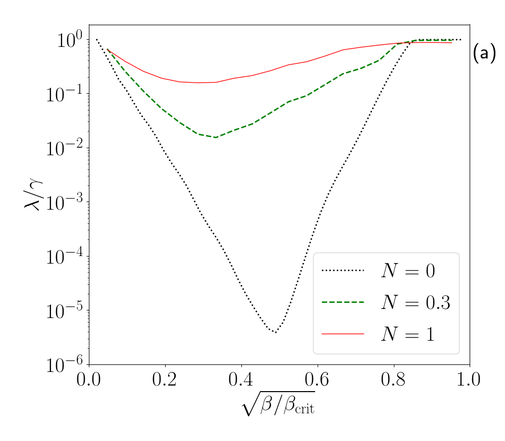
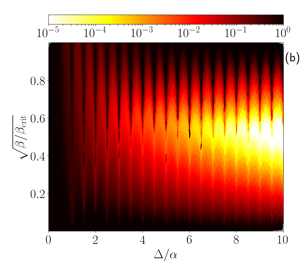
Figure 8: (a) The lowest eigenvalue of the rate equation for $N=0,0.3,1$, and $\Delta/\alpha=9.9$. The black dotted line (green dashed line, red solid line) corresponds to $N=0$ ($N=0.3$, $N=1$). (b) The lowest eigenvalue of the rate equation for $N=0$ plotted as a function of $\Delta/\alpha$, $\beta$.

To clarify the influence of the fluctuation–induced transitions on statistical properties of the internal oscillator field, one should calculate the second–order correlation function $g^{2}(0)$:

$$g^{2}(0)\equiv\frac{\left\langle\hat{a}^{\dagger}\hat{a}^{\dagger}\hat{a}\hat{a}\right\rangle}{\left\langle\hat{a}^{\dagger}\hat{a}\right\rangle^{2}}.$$ (50)

When one of the stable states dominates, $g^{(2)}(0)\sim 1$. In a narrow region of fluctuation–induced transitions $g^{(2)}(0)$ is significantly larger. For several values of $N$, we have calculated $g^{2}(0)$ as a function of two parameters: $\sqrt{\beta}$ and $\Delta/\alpha$.

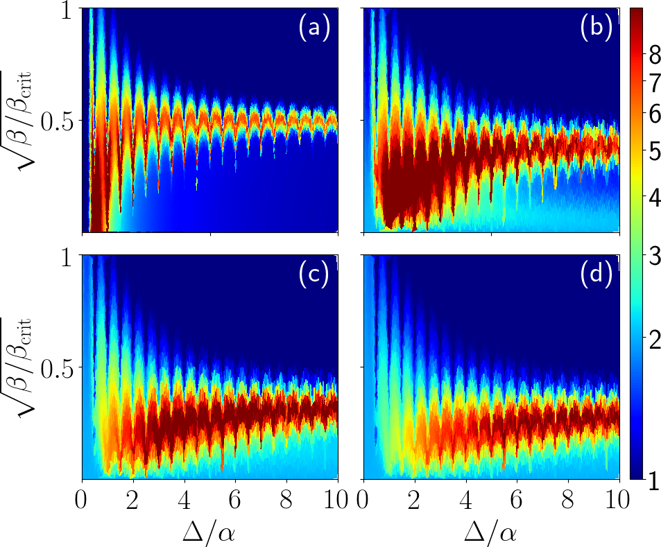
Figure 9: The correlation function $g^{2}(0)$ at different values of $N$ plotted as a function of $\Delta/\alpha$, $\beta$. (a) $N=0$ (b) $N=0.01$ (c) $N=0.05$, and (d) $N=0.1$.

For each $\Delta/\alpha$, the correlation function has similar dependence on $\sqrt{\beta}$: there is a sharp peak at some value of $\sqrt{\beta/\beta_{\mathrm{crit}}}$ between $0$ and $1$, which indicates the change of the most probable state. However, the peak is not placed at $\sqrt{\beta/\beta_{\mathrm{crit}}}\approx 0.29$ as the classical FPE predicts. Its position is an oscillating function of $\Delta/\alpha$ with sharp minima when $2\Delta/\alpha$ is an integer, which corresponds to enhanced tunneling between degenerate quasienergy states. The amplitude of oscillations decreases as $2\Delta/\alpha$ increases, when one approaches the quasiclassical limit. This fact points to the quantum nature of these oscillations.

IV Conclusions

We have derived the quasiclassical kinetic equations for the probability distribution over quasienergy states of a nonlinear driven oscillator, taking into account the tunneling effects. The stationary distribution for a wide range of system parameters and the typical relaxation rate have been determined. It was shown that the relaxation consists of two stages. At first, the relaxation to the quasi–stationary distribution occurs in each region of the phase space at time scales determined by the inverse damping constant. Then, at exponentially large times, the probability distribution evolves to the true stationary one. The relaxation to the true stationary state happens due to fluctuation–induced transitions between the quasiclassical stable states. In the classical limit, if tunneling is neglected, there exists a universal threshold value of the field intensity responsible for switching between the most probable stable states of the system. Taking into account the tunneling effects renders this value non–universal. The tunneling transitions lead to a decrease of the threshold value of external field intensity and to an up to one order of magnitude increase of the fluctuation–induced transition rate between the stable states in the threshold area.

For a driven quantum nonlinear oscillator, we demonstrated that the quasienergy state corresponding to the classical higher amplitude stable state is squeezed. The degree of squeezing is determined by the ratio of nonlinearity and detuning, and the uncertainty of one of the oscillator quadratures can be much lower than the usual quantum limit.

As tunneling transitions increase the occupation of the higher amplitude stable state, the generation of squeezed states can be enhanced in the presence of tunneling effects.

Also we demonstrated that the quasienergy states become superpositions of trajectories from different regions of the phase space. This happens whenever the detuning is an integer or half–integer multiple of the nonlinear shift per quantum. This happens due to a multi–photon resonance between the real eigenstates of the nonlinear oscillator. It was shown that such resonance can be described in terms of tunneling between the quasienergy states in different regions of the classical phase space.

The kinetics of the quantum oscillator was investigated using the quantum master equation. It was shown that in the limit of large detuning–nonlinearity ratio, large number of thermal photons and in the absence of multi–quantum resonance, the classical FPE in the quasienergy space is a continuous limit of the quantum master equation. Importantly, a large value of the detuning–nonlinearity ratio is not sufficient for the validity of the classical FPE, because at a weak noise the quantum effects become especially pronounced. The relaxation rate and the threshold intensity of the external field are both very sensitive to the detuning–nonlinearity ratio. At an integer or half–integer detuning–nonlinearity ratio, the relaxation rate can increase up to several orders of magnitude and the threshold value of the external field intensity shifts towards lower values. In this case, tunneling between degenerate quasienergy states and the multi–photon resonant transitions between the original states of the nonlinear oscillator can be treated as the same effect.

Finally, it was shown that the second–order correlation function of the internal field strongly rises near the threshold pumping intensity, which indicates super–Poissonian statistics of the internal oscillator field.

*

Appendix A The coefficients of the classical Fokker–Planck equation

The coefficients of the classical FPE are defined as follows:

$$\begin{gathered}K(E)=\frac{i}{2}\oint a\,da^{*}-a^{*}\,da,\\ D(E)=\frac{i}{2}\oint\frac{\partial H}{\partial a}da-\frac{\partial H}{\partial a^{*}}da^{*},\\ T(E)=\int da^{*}da\,\delta(E-H(a^{*},a)).\\ \end{gathered}$$ (51)

For them, we obtained the following integral representations:

$$T(E)=\int\frac{dt}{\sqrt{2f^{2}t-\left(E+\frac{t}{2}-\frac{t^{2}}{8}\right)^{2}}},$$ (52)

$$K_{i}(E)=\int\frac{3t^{2}/16-t/4+E/2}{\sqrt{2f^{2}t-\left(E+\frac{t}{2}-\frac{t^{2}}{8}\right)^{2}}}dt,$$ (53)

$$D_{i}(E)=\int\frac{t^{3}/16-t^{2}/8+Et/2+f^{2}-E}{\sqrt{2f^{2}t-\left(E+\frac{t}{2}-\frac{t^{2}}{8}\right)^{2}}}dt.$$ (54)

The limits of the integration are the roots or the equation

$$2f^{2}t-\left(E+\frac{t}{2}-\frac{t^{2}}{8}\right)^{2}=0.$$

For energies $E_{2}<E<E_{\mathrm{sep}}$ corresponding to the classical region $2$, this equation has only two real roots. For energies $E_{\mathrm{sep}}<E<E_{1}$ corresponding to regions 1 and 3, there are four real roots. $t_{1}<t_{2}<t_{3}<t_{4}$. To obtain $T_{1}$, $K_{1}$ and $D_{1}$, the limits of integration should be $t_{1}$, $t_{2}$, and for $T_{3}$, $K_{3}$, $D_{3}$, they should be $t_{3}$, $t_{4}$. Finally, for $E>E_{1}$, which corresponds only to region 3, there are two real roots once again.