A Newton method for harmonic mappings in the plane

Abstract

We present an iterative root finding method for harmonic mappings in the complex plane, which is a generalization of Newton’s method for analytic functions. The complex formulation of the method allows an analysis in a complex variables spirit. For zeros close to poles of $f=h+\overline{g}$ we construct initial points for which the harmonic Newton iteration is guaranteed to converge. Moreover, we study the number of solutions of $f(z)=\eta$ close to the critical set of $f$ for certain $\eta\in\mathbb{C}$. We provide a Matlab implementation of the method, and illustrate our results with several examples and numerical experiments, including phase plots and plots of the basins of attraction.

Keywords:

Zeros of harmonic mappings; Newton’s method; basins of attraction; domain coloring; Wilmshurst’s conjecture; gravitational lensing.

Mathematics Subject Classification (2010):

30C55; 30D05; 31A05; 37F99; 65E05.

1 Introduction

We study harmonic mappings, i.e., functions with local decomposition

$$f(z)=h(z)+\overline{g(z)}$$ (1.1)

in the complex plane, where $h$ and $g$ are analytic. The function $f$ itself is not analytic in general, as it consists of an analytic and an anti-analytic term.

The modern treatment of harmonic mappings started from the landmark paper [7] of Clunie and Sheil-Small about univalent harmonic mappings in the plane. See also the comprehensive textbook of Duren [11]. While [11] considers univalent harmonic mappings, also the multivalent case has been intensively studied; see e.g. the collection of open problems [5] by Bshouty and Lyzzaik. Problem 3.7 in [5] deals with the maximum number of zeros of harmonic polynomials $f(z)=p(z)+\overline{q(z)}$. Wilmshurst proved an upper bound for this number and conjectured another bound depending on $\deg(p)$ and $\deg(q)$ [45]; see Section 6.1 and the more recent publications concerning Wilmshurst’s conjecture [24, 15, 19]. Khavinson and Świa̧tek [23], and Geyer [13] settled the conjecture, including sharpness, for the special case $f(z)=p(z)-\overline{z}$. Khavinson and Neumann [21] generalized these results to rational harmonic functions $f(z)=r(z)-\overline{z}$; see also [28, 26]. The sharpness of the bound in the rational case was previously known due to the astrophysicist Rhie [36]. As it turns out, harmonic mappings model gravitational lensing - an astrophysical phenomenon, where, due to deflection by massive objects, a light source seems brightened, distorted or multiplied for an observer. We refer to the expository articles [22, 34], and the survey [3]. More recent articles on harmonic mappings with applications to gravitational lensing are [4, 20, 29, 37, 38, 27, 25].

The results about the zeros of harmonic mappings published so far are more theoretical, and we are not aware of any specialized method to compute them, which may explain the lack of (numerical) examples in the respective publications. In this paper we focus on the numerical computation of zeros of harmonic mappings with a Newton method.

The global behavior of Newton’s method on $\mathbb{R}^{2}$, see e.g. [33, Ch. 7], has been less treated than the one of Newton’s method for analytic or anti-analytic functions in $\mathbb{C}$. However, the recent publications [8, 9] give new impulses to this subject. Since harmonic mappings are generalizations of both analytic and anti-analytic functions, our work may also lead to new insights on the dynamics of Newton’s method on $\mathbb{R}^{2}$. Our approach is not covered by the standard theory of complex dynamics [6, 30], nor by anti-holomorphic dynamics, see [32, 31], since the corresponding Newton map (3.7) is neither analytic nor harmonic.

The paper is organized as follows. In Section 2 we recall the definition and properties of harmonic mappings as well as Newton’s method in Banach spaces. We then derive the harmonic Newton iteration and more generally a Newton iteration in complex notation for non-analytic but real differentiable functions in Section 3. We investigate zeros of $f=h+\overline{g}$ close to poles in Section 4. In particular, we construct initial points from the coefficients of the Laurent series of $h$ and $g$, for which the harmonic Newton iteration is guaranteed to converge to zeros of $f$. In Section 5, we study solutions of $f(z)=\eta$, where $z$ is close to a singular zero $z_{0}$ of $f$, and for certain small $\eta\in\mathbb{C}$. In Section 6, we consider several (numerical) examples. Finally, we give a summary and discuss possible future research in Section 7.

2 Mathematical background

In this section we recall properties of harmonic mappings and classical convergence results for Newton’s method.

2.1 Harmonic mappings

The Wirtinger derivatives of a complex function $f$ are

$$\partial_{z}f=\frac{1}{2}(\partial_{x}f-i\partial_{y}f),\quad\partial_{\overline{z}}f=\frac{1}{2}(\partial_{x}f+i\partial_{y}f),$$

where $z=x+iy$ with $x,y\in\mathbb{R}$; see [11, Section 1.2], [35, Section 1.4], or [44, p. 144]. They satisfy

$$\partial_{x}f=\partial_{z}f+\partial_{\overline{z}}f,\quad\partial_{y}f=i(\partial_{z}f-\partial_{\overline{z}}f),\quad\partial_{\overline{z}}\overline{f(z)}=\overline{\partial_{z}f(z)}.$$ (2.1)

A harmonic mapping is a function $f:\Omega\to\mathbb{C}$ defined on an open set $\Omega\subseteq\mathbb{C}$ and with

$$\Delta f=\partial_{xx}f+\partial_{yy}f=4\partial_{\overline{z}}\partial_{z}f=0.$$

Such a function has a local decomposition $f(z)=h(z)+\overline{g(z)}$, where $h$ and $g$ are analytic functions of $z$ which are unique up to an additive constant [12, p. 412] or [11, p. 7]. The Jacobian of a harmonic mapping $f$ at $z\in\Omega$ is

$$J_{f}(z)=\lvert\partial_{z}f(z)\rvert^{2}-\lvert\partial_{\overline{z}}f(z)\rvert^{2}=\lvert h^{\prime}(z)\rvert^{2}-\lvert g^{\prime}(z)\rvert^{2}.$$ (2.2)

We call $f$ sense-preserving (or orientation-preserving) at $z\in\Omega$ if $J_{f}(z)>0$, sense-reversing if $J_{f}(z)<0$, and singular if $J_{f}(z)=0$, and similarly for zeros of $f$, e.g., $z_{0}$ is a singular zero of $f$ if $J_{f}(z_{0})=0$. The points where $f$ is singular form the critical set

$$\mathcal{C}=\{z\in\mathbb{C}:J_{f}(z)=0\}.$$ (2.3)

One way to visualize complex functions are phase plots, where the domain is colored according to the phase $f(z)/\lvert f(z)\rvert$ of $f$. We use the standard color scheme described in [44] for all phase plots, and accordingly use white for the value $\infty$ (e.g., for poles of $h$ or $g$) and black for zeros; see Figure 1. A comprehensive discussion of phase plots can be found in [44].

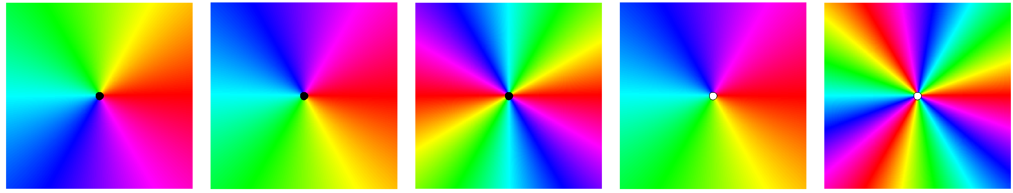
Figure 1: Phase plots of $z$, $\overline{z}$, $z^{2}$, $1/z$ and $1/\overline{z}^{3}$ (from left to right).

Example 2.1

Consider the rational harmonic function

$$f(z)=h(z)+\overline{g(z)}=\frac{z^{n-1}}{z^{n}-r^{n}}-\overline{z},$$ (2.4)

where $h$ has the poles $re^{i2\pi k/n}$, $k=0,1,\ldots,n-1$. The function $f$ has $3n+1$ zeros provided that $r>0$ is sufficiently small; see [28] for a detailed analysis. Figure 2 shows the phase plot of $f$ for $n=3$ and $r=0.6$, the $3$ poles of $f$ and the $10$ zeros. Depending on the orientation, the phase plot of $f$ near a zero looks like the phase plot of $z$ (sense-preserving) or $\overline{z}$ (sense-reversing) near $0$ in Figure 1.

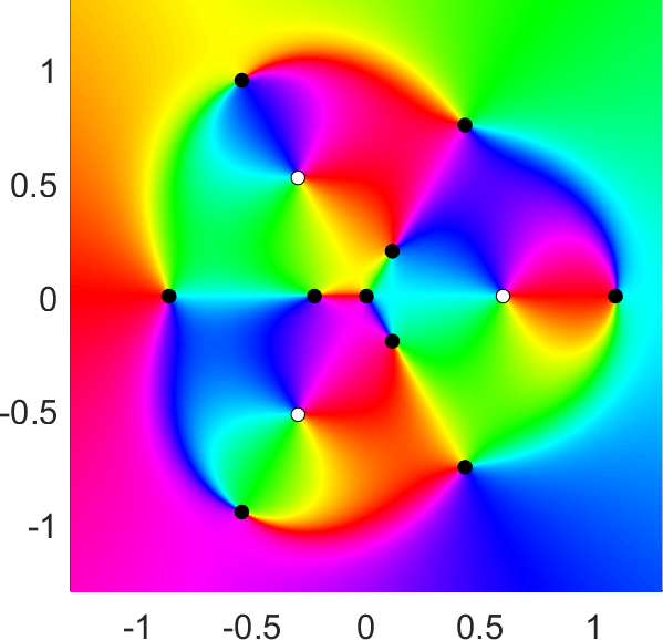
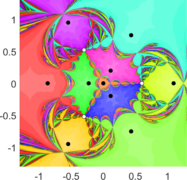
Figure 2: Left: Phase plot of $f(z)=z^{2}/(z^{3}-0.6^{3})-\overline{z}$; see Example 2.1. White dots are the poles, black dots are the zeros. Right: Basins of attraction of the zeros of $f$ in the harmonic Newton method; see Section 3 below.

2.2 Newton’s method in Banach spaces

Let $F:D\to Y$, $D\subseteq X$ open, be a continuously Fréchet differentiable map between two Banach spaces $X$, $Y$. The Newton iteration with initial point $x_{0}\in D$ is

$$x_{k+1}=x_{k}-F^{\prime}(x_{k})^{-1}F(x_{k}),\quad k\geq 0.$$ (2.5)

Under some regularity conditions, the sequence of Newton iterates $(x_{k})_{k}$ is quadratically convergent ($\lVert x_{k+1}-x_{*}\rVert\leq\text{const}\cdot\lVert x_{k}-x_{*}\rVert^{2}$), if $x_{0}$ is sufficiently close to a zero of $F$; see e.g. [46, Prop. 5.1]. The next two theorems quantify “sufficiently close”.

The Newton-Kantorovich theorem guarantees existence of a zero close to the initial point of the Newton iteration. In the following, $B(x_{0};r)$ and $\overline{B}(x_{0};r)$ denote the open and closed balls with center $x_{0}$ and radius $r$.

Theorem 2.2 (Newton-Kantorovich, [10, Thm. 2.1])

Let $F:D\to Y$ be a continuously Fréchet differentiable map with $D\subseteq X$ open and convex. For an initial point $x_{0}\in D$ let $F^{\prime}(x_{0})$ be invertible. Suppose that

$$\lVert F^{\prime}(x_{0})^{-1}F(x_{0})\rVert \leq\alpha,$$

$$\lVert F^{\prime}(x_{0})^{-1}(F^{\prime}(y)-F^{\prime}(x))\rVert \leq\omega_{0}\lVert y-x\rVert\quad\text{for all }x,y\in D.$$

Let $h_{0}=\alpha\omega_{0}$ and $\rho=(1-\sqrt{1-2h_{0}})/\omega_{0}$, and suppose that

$$h_{0}\leq\frac{1}{2}\quad\text{and}\quad\overline{B}(x_{0};\rho)\subseteq D.$$

Then the sequence $(x_{k})_{k}$ of Newton iterates is well defined, remains in $\overline{B}(x_{0};\rho)$, and converges to some $x_{*}$ with $F(x_{*})=0$. If $h_{0}<\frac{1}{2}$, then the convergence is quadratic.

The refined Newton-Mysovskii theorem guarantees uniqueness of a zero, but not its existence. Given a zero, it quantifies a neighborhood in which the Newton iteration will converge, as well as a constant for the quadratic convergence estimate.

Theorem 2.3 (refined Newton-Mysovskii theorem, [10, Thm. 2.3])

Let $F:D\to\mathbb{R}^{n}$ be a continuously differentiable map with $D\subseteq\mathbb{R}^{n}$ open and convex. Suppose that $F^{\prime}(x)$ is invertible for each $x\in D$. Suppose that

$$\lVert F^{\prime}(x)^{-1}(F^{\prime}(y)-F^{\prime}(x))(y-x)\rVert\leq\omega\lVert y-x\rVert^{2}\quad\text{for all }x,y\in D.$$ (2.6)

Let $F(x)=0$ have a solution $x_{*}\in D$. For the initial point $x_{0}$ suppose that $\overline{B}(x_{*};\lVert x_{0}-x_{*}\rVert)\subseteq D$ and that

$$\lVert x_{0}-x_{*}\rVert<\frac{2}{\omega}.$$

Then the sequence of Newton iterates $(x_{k})_{k}$ is well defined, remains in the open ball $B(x_{*};\lVert x_{0}-x_{*}\rVert)$, converges to $x_{*}$, and fulfills

$$\lVert x_{k+1}-x_{*}\rVert\leq\frac{\omega}{2}\lVert x_{k}-x_{*}\rVert^{2}.$$

Moreover, the solution $x_{*}$ is unique in $B(x_{*};2/\omega)$.

We frequently use Landau’s $\mathcal{O}$-notation for complex functions. By $f(z)+\mathcal{O}(z^{k})$ we mean an expression $f(z)+\psi(z)$, where $\psi(z)\in\mathcal{O}(z^{k})$, i.e., $\lvert\psi(z)/z^{k}\rvert$ is bounded from above by a constant (usually for $z\to 0$ or $z\to\infty$, depending on the context).

Remark 2.4

Using the Taylor expansion $\sqrt{1+z}=1+\frac{z}{2}+\mathcal{O}(z^{2})$, we find the asymptotic expression

$$\rho=\frac{1-\sqrt{1-2h_{0}}}{\omega_{0}}=\frac{1-(1-h_{0}+\mathcal{O}(h_{0}^{2}))}{\omega_{0}}=\alpha+\mathcal{O}(\alpha h_{0}),$$ (2.7)

in Theorem 2.2, whenever the Kantorovich quantity $h_{0}$ is sufficiently small.

While we only require the above results, other convergence results for Newton’s method in Banach spaces exist; see e.g. [39, 43].

3 The harmonic Newton method

We derive the harmonic Newton iteration and discuss its implementation.

3.1 The Newton iteration in the plane in complex notation

Let $f:\Omega\to\mathbb{C}$ be (continuously) differentiable with respect to $x=\operatorname{Re}(z)$ and $y=\operatorname{Im}(z)$, where we do not require for the moment that $f$ is analytic or harmonic. We identify $\mathbb{C}$ with $\mathbb{R}^{2}$, and $f$ with

$$F:\Omega\to\mathbb{R}^{2},\quad F(z)=\begin{bmatrix}\operatorname{Re}(f(z))\\ \operatorname{Im}(f(z))\end{bmatrix},\quad z=x+iy,$$ (3.1)

which is a smooth function of $x$ and $y$.

Since $\operatorname{Re}$ and $\operatorname{Im}$ are $\mathbb{R}$-linear and continuous, they commute with $\partial_{x}$ and $\partial_{y}$. Thus, $F^{\prime}(z)$ has the matrix representation

$$F^{\prime}(z)=\begin{bmatrix}\operatorname{Re}(\partial_{z}f(z))+\operatorname{Re}(\partial_{\overline{z}}f(z))&-\operatorname{Im}(\partial_{z}f(z))+\operatorname{Im}(\partial_{\overline{z}}f(z))\\ \operatorname{Im}(\partial_{z}f(z))+\operatorname{Im}(\partial_{\overline{z}}f(z))&\operatorname{Re}(\partial_{z}f(z))-\operatorname{Re}(\partial_{\overline{z}}f(z))\end{bmatrix},$$ (3.2)

where we used the Wirtinger derivatives (2.1). The inverse of $F^{\prime}(z)$ is

$$F^{\prime}(z)^{-1}=\frac{1}{J_{f}(z)}\begin{bmatrix}\operatorname{Re}(\partial_{z}f(z))-\operatorname{Re}(\partial_{\overline{z}}f(z))&\operatorname{Im}(\partial_{z}f(z))-\operatorname{Im}(\partial_{\overline{z}}f(z))\\ -\operatorname{Im}(\partial_{z}f(z))-\operatorname{Im}(\partial_{\overline{z}}f(z))&\operatorname{Re}(\partial_{z}f(z))+\operatorname{Re}(\partial_{\overline{z}}f(z))\end{bmatrix},$$

provided $J_{f}(z)=\lvert\partial_{z}f(z)\rvert^{2}-\lvert\partial_{\overline{z}}f(z)\rvert^{2}\neq 0$; compare (2.2). We identify $F^{\prime}(z)$ and its inverse with the $\mathbb{R}$-linear maps on $\mathbb{C}$

$$F^{\prime}(z)(w) =(\partial_{z}f(z))w+(\partial_{\overline{z}}f(z))\overline{w},$$

$$F^{\prime}(z)^{-1}(w) =\frac{1}{J_{f}(z)}(\overline{\partial_{z}f(z)}w-(\partial_{\overline{z}}f(z))\overline{w}).$$

Then the Newton iteration (2.5) for $F$ can be rewritten in $\mathbb{C}$ as

$$z_{k+1}=z_{k}-\frac{\overline{\partial_{z}f(z_{k})}f(z_{k})-\partial_{\overline{z}}f(z_{k})\overline{f(z_{k})}}{\lvert\partial_{z}f(z_{k})\rvert^{2}-\lvert\partial_{\overline{z}}f(z_{k})\rvert^{2}},\quad k\geq 0.$$ (3.3)

3.2 The harmonic Newton iteration

For a harmonic mapping with local decomposition $f=h+\overline{g}$, we have $\partial_{z}f(z)=h^{\prime}(z)$ and $\partial_{\overline{z}}f(z)=\partial_{\overline{z}}\overline{g(z)}=\overline{g^{\prime}(z)}$ with (2.1), so that $F^{\prime}(z)$ and $F^{\prime}(z)^{-1}$ can be identified with

$$F^{\prime}(z)(w) =h^{\prime}(z)w+\overline{g^{\prime}(z)w},$$ (3.4)

$$F^{\prime}(z)^{-1}(w) =\frac{1}{J_{f}(z)}(\overline{h^{\prime}(z)}w-\overline{g^{\prime}(z)w}),$$ (3.5)

and the Newton iteration (3.3) takes the form

$$z_{k+1}=z_{k}-\frac{\overline{h^{\prime}(z_{k})}f(z_{k})-\overline{g^{\prime}(z_{k})f(z_{k})}}{\lvert h^{\prime}(z_{k})\rvert^{2}-\lvert g^{\prime}(z_{k})\rvert^{2}},\quad k\geq 0,$$ (3.6)

which we call the harmonic Newton iteration. It reduces to the classical Newton iteration $z_{k+1}=z_{k}-f(z_{k})/f^{\prime}(z_{k})$ when $f$ is analytic ($f=h$). Similarly, if $f$ is anti-analytic ($f=\overline{g}$), the iteration simplifies to $z_{k+1}=z_{k}-g(z_{k})/g^{\prime}(z_{k})$. Hence, the harmonic Newton iteration (3.6) is a natural generalization of the classical Newton iteration.

We define the harmonic Newton map

$$H_{f}:\Omega\setminus\mathcal{C}\to\mathbb{C},\quad z\mapsto H_{f}(z)=z-\frac{\overline{h^{\prime}(z)}f(z)-\overline{g^{\prime}(z)f(z)}}{\lvert h^{\prime}(z)\rvert^{2}-\lvert g^{\prime}(z)\rvert^{2}},$$ (3.7)

which is in general neither analytic nor harmonic. Note that $z_{*}\in\Omega\setminus\mathcal{C}$ is a fixed point of $H_{f}$ if and only if $z_{*}$ is a non-singular zero of $f$. Borrowing notation from complex dynamics, see e.g. [6, 30], we define the basin of attraction of a zero $z_{*}$ of $f$ as

$$A(z_{*})=\{z\in\mathbb{C}:\lim_{k\to\infty}H_{f}^{k}(z)=z_{*}\},$$

where $H_{f}^{1}=H_{f}$ and $H_{f}^{k}=H_{f}\circ H_{f}^{k-1}$ for $k\geq 2$. Note that the basin of attraction of a non-singular zero $z_{*}$ contains an open neighborhood of $z_{*}$, by the local convergence of Newton’s method. For singular zeros this need not be the case; see Example 6.3.

To visualize the dynamics of the harmonic Newton map, we use the following standard domain coloring technique; see, e.g., [14, 42]. We color every point according to which basin it belongs to. The color level indicates the number of iterations, the darker the more iterations were required. Points where the harmonic Newton iteration does not converge are colored in black; see Figure 2.

3.3 Implementation

Algorithm 1 Harmonic Newton method

Input: $f$, $h^{\prime}$, $g^{\prime}$, and $z_{0}\in\mathbb{C}$, $N\in\mathbb{N}$, $\varepsilon_{f},\varepsilon_{z}>0$
Output: approximated zero of $f$

1:for $k=0,\dots,N-1$ do

2:     $\displaystyle z_{k+1}=z_{k}-\frac{\overline{h^{\prime}(z_{k})}f(z_{k})-\overline{g^{\prime}(z_{k})f(z_{k})}}{\lvert h^{\prime}(z_{k})\rvert^{2}-\lvert g^{\prime}(z_{k})\rvert^{2}}$

3:     if $\lvert f(z_{k+1})\rvert<\varepsilon_{f}$ or $\lvert z_{k+1}-z_{k}\rvert<\varepsilon_{z}\lvert z_{k+1}\rvert$ then

4:         return $z_{k+1}$

5:     end if

6:end for

7:return $z_{N}$

Following Higham [17, Sect. 25.5], we stop the harmonic Newton iteration when the residual $\lvert f(z_{k})\rvert$ or the relative difference between two iterates $\lvert z_{k+1}-z_{k}\rvert/\lvert z_{k+1}\rvert$ are less than given tolerances, or when a prescribed maximum number of steps has been performed. This gives the harmonic Newton method; see Algorithm 1. Note that, when $f(z_{*})=0$ and $\lvert z_{k}-z_{*}\rvert$ is sufficiently small, we have $\lvert z_{k+1}-z_{*}\rvert\leq 2c\lvert z_{k+1}-z_{k}\rvert^{2}$, where $c$ is the constant from the (local) quadratic convergence of the Newton method; see [17, Sect. 25.5].

Our MATLAB implementation of Algorithm 1 is displayed in Figure 3. To apply a harmonic Newton step not only to a single point, but to a vector or matrix of points, we vectorize the iteration (3.6), see lines 25–26. This also requires vectorized function handles for $f$, $h^{\prime}$, $g^{\prime}$. Vectorization is particularly useful when we have several initial points, since applying the method to a matrix of initial points is usually faster than applying it to each point individually. When all points are iterated simultaneously, some might already have converged while others have not. However, further iterating a point that has numerically converged can be harmful in finite precision, e.g., when a point is close to the critical set, a further Newton step may lead to division by zero. Hence, we stop the iteration individually for each point, by removing them from the list of active points; see lines 15 and 33.

⬇

function [z, numiter] = harmonicNewton(f, dh, dg, z, maxit, restol, steptol)

% Set default values:

if ((nargin < 5) || isempty(maxit)), maxit = 50; end

if ((nargin < 6) || isempty(restol)), restol = 1e-14; end

if ((nargin < 7) || isempty(steptol)), steptol = 1e-14; end

% Setup

active = 1:numel(z); % track which points to iterate

numiter = (maxit+1)*ones(size(z)); % number of iterations

% Check initial points:

fz = f(z);

converged = (abs(fz) < restol); % already converged

diverged = (isnan(fz) | isinf(fz)); % NaN or Inf

numiter(converged) = 0; % no Newton steps required

active(converged | diverged) = []; % do not further iterate

fz = fz(active);

% Harmonic Newton iteration:

for kk = 1:maxit

if (isempty(active)), return, end % every point has converged

zold = z(active);

% Evaluate functions:

dhz = dh(zold);

dgz = dg(zold);

% Newton step:

z(active) = zold …

- (conj(dhz).*fz - conj(dgz.*fz))./(abs(dhz).^2 - abs(dgz).^2);

% Convergence check:

fz = f(z(active));

converged = (abs(fz) < restol) | …

(abs(z(active) - zold) < steptol*abs(zold));

diverged = (isnan(fz) | isinf(fz)); % NaN or inf

numiter(active(converged)) = kk; % took kk iterations

active(converged | diverged) = []; % remove converged points

fz(converged | diverged) = []; % remove converged points

end

end

Figure 3: MATLAB implementation of the harmonic Newton method used in the examples.

Note that computing the next iterate in (3.6) requires only the three function evaluations $f(z_{k})$, $h^{\prime}(z_{k})$ and $g^{\prime}(z_{k})$.

Computing the next iterate by (3.6) or by solving the $2\times 2$ real linear algebraic system corresponding to

$$F^{\prime}(z_{k})(z_{k+1}-z_{k})=-F(z_{k})$$ (3.8)

with (3.2) are equivalent in exact arithmetic. This is not the case in finite precision, where the Jacobian $J_{f}(z)$ can be numerically zero, although $z$ is not on the critical set. To avoid division by zero, it is preferable to compute the next iterate by solving (3.8), instead of inverting $F^{\prime}(z_{k})$ explicitly. However, we use (3.6) in our numerical experiments (except in Example 4.1), see line 2 in Algorithm 1 and lines 25–26 in Figure 3, because (3.6) can be easily vectorized.

4 Finding zeros close to poles

The complex formulation (3.6) makes the harmonic Newton iteration amenable to analysis in a complex variables spirit. We investigate zeros of harmonic mappings $f=h+\overline{g}$ close to poles $z_{0}$, i.e., points where $\lim_{z\to z_{0}}\lvert f(z)\rvert=\infty$; see [40, Def. 2.1]. More precisely, we construct initial points from the Laurent coefficients of $h$ and $g$, for which the harmonic Newton iteration is guaranteed to converge to zeros of $f$. We start with an example.

Example 4.1

We consider $f(z)=\tan(z)-\overline{z}$; see Figure 4.

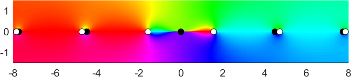
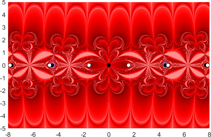
Figure 4: The function $f(z)=\tan(z)-\overline{z}$ from Example 4.1. Top: Phase plot, zeros (black dots), poles (white dots). Bottom: Basins of attraction.

The function has a singular zero at the origin, and one (real) zero close to each pole of the tangent, except $\pm\frac{\pi}{2}$. To compute the zeros of $f$ we apply the harmonic Newton method to a grid of initial points in $[-8,8]\times[-2,2]$ with mesh size $0.2$, tolerances $10^{-14}$, and with up to $50$ steps. The residual at our computed zeros satisfies $\lvert f(z_{k})\rvert\leq 1.5600\cdot 10^{-13}$.

Since the Jacobian $J_{f}(z)=\lvert 1+\tan(z)^{2}\rvert^{2}-1$ is numerically zero for $\lvert z\rvert\leq 10^{-9}$, we use (3.8) instead of (3.6) to compute the basins of attraction in this example. We observe that the basin of $0$ is huge, while the basins of zeros close to poles are small. Moreover, the size of the basins decreases for larger poles, and the poles seem to be on the boundary of the basins.

Note that the black points on the imaginary axis are due to a numerically vanishing Jacobian, as above. Analytically, the harmonic Newton map is

$$H_{f}(iy)=i\left(y-\frac{y+\tanh(y)}{1+\operatorname{sech}(y)^{2}}\right)\quad\text{for }y\in\mathbb{R},$$

and one can prove that every point on the imaginary axis converges to $0$.

Next, we construct initial points for which the harmonic Newton iteration converges to zeros close to a pole. For this, we need the following lemma.

Lemma 4.2

The equation $az+\overline{bz}=c$ has a unique solution if and only if $\lvert a\rvert\neq\lvert b\rvert$. In that case, the unique solution is $z=\frac{\overline{a}c-\overline{bc}}{\lvert a\rvert^{2}-\lvert b\rvert^{2}}$.

Splitting $az+\overline{bz}=c$ in its real and imaginary part yields a real $2\times 2$ linear algebraic system with determinant $\lvert a\rvert^{2}-\lvert b\rvert^{2}$, from which we obtain the assertion.

To apply the Newton-Kantorovich theorem to the harmonic Newton iteration (3.6), we identify $\mathbb{C}$ with $\mathbb{R}^{2}$ as in Section 3.1. First, we derive bounds for the constants $\alpha$ and $\omega_{0}$ in Theorem 2.2 using the formulas for $F^{\prime}$ and $(F^{\prime})^{-1}$ from (3.4) and (3.5). We find

$$\lvert F^{\prime}(z_{0})^{-1}(w)\rvert\leq\frac{\lvert h^{\prime}(z_{0})\rvert+\lvert g^{\prime}(z_{0})\rvert}{\big{\lvert}\lvert h^{\prime}(z_{0})\rvert^{2}-\lvert g^{\prime}(z_{0})\rvert^{2}\big{\rvert}}\lvert w\rvert=\frac{\lvert w\rvert}{\big{\lvert}\lvert h^{\prime}(z_{0})\rvert-\lvert g^{\prime}(z_{0})\rvert\big{\rvert}},$$

and so

$$\lvert F^{\prime}(z_{0})^{-1}(F(z_{0}))\rvert\leq\frac{\lvert f(z_{0})\rvert}{\big{\lvert}\lvert h^{\prime}(z_{0})\rvert-\lvert g^{\prime}(z_{0})\rvert\big{\rvert}}\leq\alpha$$ (4.1)

and

$$\lVert F^{\prime}(z_{0})^{-1}(F^{\prime}(y)-F^{\prime}(x))\rVert =\max_{\lvert z\rvert=1}\lvert F^{\prime}(z_{0})^{-1}(F^{\prime}(y)-F^{\prime}(x))(z)\rvert$$

$$\leq\frac{\max_{\lvert z\rvert=1}(\lvert h^{\prime}(y)-h^{\prime}(x)\rvert+\lvert g^{\prime}(y)-g^{\prime}(x)\rvert)\lvert z\rvert}{\big{\lvert}\lvert h^{\prime}(z_{0})\rvert-\lvert g^{\prime}(z_{0})\rvert\big{\rvert}}$$

$$\leq\frac{\sup_{t\in D}\lvert h^{\prime\prime}(t)\rvert+\sup_{t\in D}\lvert g^{\prime\prime}(t)\rvert}{\big{\lvert}\lvert h^{\prime}(z_{0})\rvert-\lvert g^{\prime}(z_{0})\rvert\big{\rvert}}\lvert y-x\rvert$$

$$\leq\omega_{0}\lvert y-x\rvert.$$ (4.2)

Next we present the main result of this section.

Theorem 4.3

Let $f=h+\overline{g}$, where

$$h(z)=\sum_{k=-n}^{\infty}a_{k}(z-z_{0})^{k},\quad g(z)=\sum_{k=-n}^{\infty}b_{k}(z-z_{0})^{k},$$

with $n\geq 1$, and $\lvert a_{-n}\rvert\neq\lvert b_{-n}\rvert$. Suppose that $c=-(a_{0}+\overline{b}_{0})\neq 0$, and let $z_{1},\ldots,z_{n}$ be the $n$ solutions of

$$(z-z_{0})^{n}=\frac{\lvert a_{-n}\rvert^{2}-\lvert b_{-n}\rvert^{2}}{\overline{a}_{-n}c-\overline{b}_{-n}\overline{c}}.$$ (4.3)

We then have for sufficiently large $\lvert c\rvert$:

1. There exist $n$ distinct zeros of $f$ near $z_{0}$.

2. The zeros in 1. are the limits of the harmonic Newton iteration with initial points $z_{1},\ldots,z_{n}$.

We apply the Newton-Kantorovich theorem for each of the $n$ initial points $z_{j}$. Without loss of generality, we assume $z_{0}=0$. Then “$\lvert c\rvert$ sufficiently large” is equivalent to “$\lvert z_{j}\rvert$ sufficiently small”.

The cases $n=1$ and $n\geq 2$ differ slightly, and we begin with $n\geq 2$. First, we determine $\alpha$ from (4.1). With (4.3) and Lemma 4.2 we obtain

$$a_{-n}(z_{j}-z_{0})^{-n}+\overline{b}_{-n}(z_{j}-z_{0})^{-n}=c=-(a_{0}+\overline{b}_{0}),$$

and

$$\lvert f(z_{j})\rvert\leq(\lvert a_{-n+1}\rvert+\lvert b_{-n+1}\rvert)\lvert z_{j}\rvert^{-n+1}+\mathcal{O}(\lvert z_{j}\rvert^{-n+2}),$$ (4.4)

and from

$$h^{\prime}(z)=-na_{-n}z^{-n-1}+\mathcal{O}(z^{-n}),\quad g^{\prime}(z)=-nb_{-n}z^{-n-1}+\mathcal{O}(z^{-n}),$$

also

$$\big{\lvert}\lvert h^{\prime}(z_{j})\rvert-\lvert g^{\prime}(z_{j})\rvert\big{\rvert}=n\big{\lvert}\lvert a_{-n}\rvert-\lvert b_{-n}\rvert\big{\rvert}\lvert z_{j}\rvert^{-n-1}+\mathcal{O}(\lvert z_{j}\rvert^{-n}),$$

so that

$$\begin{split}\frac{\lvert f(z_{j})\rvert}{\big{\lvert}\lvert h^{\prime}(z_{j})\rvert-\lvert g^{\prime}(z_{j})\rvert\big{\rvert}}&\leq\frac{(\lvert a_{-n+1}\rvert+\lvert b_{-n+1}\rvert)\lvert z_{j}\rvert^{-n+1}+\mathcal{O}(\lvert z_{j}\rvert^{-n+2})}{n\big{\lvert}\lvert a_{-n}\rvert-\lvert b_{-n}\rvert\big{\rvert}\lvert z_{j}\rvert^{-n-1}+\mathcal{O}(\lvert z_{j}\rvert^{-n})}\\ &=\frac{\lvert a_{-n+1}\rvert+\lvert b_{-n+1}\rvert}{n\big{\lvert}\lvert a_{-n}\rvert-\lvert b_{-n}\rvert\big{\rvert}}\lvert z_{j}\rvert^{2}+\mathcal{O}(\lvert z_{j}\rvert^{3})=\alpha.\end{split}$$

Here we used that $1/(1+\mathcal{O}(x))=1+\mathcal{O}(x)$ for $x\to 0$.

Next we determine $\omega_{0}$ from (4.2). Let $D=\{z\in\mathbb{C}:\lvert z-z_{j}\rvert<q\lvert z_{j}\rvert\}$ for some $0<q<1$. From

$$h^{\prime\prime}(z)=n(n+1)a_{-n}z^{-n-2}+\mathcal{O}(z^{-n-1}),$$

we get

$$\sup_{t\in D}\lvert h^{\prime\prime}(t)\rvert\leq n(n+1)\lvert a_{-n}\rvert((1-q)\lvert z_{j}\rvert)^{-n-2}+\mathcal{O}(\lvert z_{j}\rvert^{-n-1}),$$

and similarly for $g$. Then

$$\begin{split}&\frac{\sup_{t\in D}\lvert h^{\prime\prime}(t)\rvert+\sup_{t\in D}\lvert g^{\prime\prime}(t)\rvert}{\big{\lvert}\lvert h^{\prime}(z_{j})\rvert-\lvert g^{\prime}(z_{j})\rvert\big{\rvert}}\\ &\leq\frac{n(n+1)(\lvert a_{-n}\rvert+\lvert b_{-n}\rvert)((1-q)\lvert z_{j}\rvert)^{-n-2}+\mathcal{O}(\lvert z_{j}\rvert^{-n-1})}{n\big{\lvert}\lvert a_{-n}\rvert-\lvert b_{-n}\rvert\big{\rvert}\lvert z_{j}\rvert^{-n-1}+\mathcal{O}(\lvert z_{j}\rvert^{-n})}\\ &=\frac{(n+1)(\lvert a_{-n}\rvert+\lvert b_{-n}\rvert)(1-q)^{-n-2}}{\big{\lvert}\lvert a_{-n}\rvert-\lvert b_{-n}\rvert\big{\rvert}}\lvert z_{j}\rvert^{-1}+\mathcal{O}(1)=\omega_{0},\end{split}$$

and $h_{0}=\alpha\omega_{0}=\mathcal{O}(\lvert z_{j}\rvert)$. Hence, for any $0<q<1$, we have $h_{0}<\frac{1}{2}$ for sufficiently small $\lvert z_{j}\rvert$.

It remains to show that $\rho<q\lvert z_{j}\rvert$. Using (2.7) we get

$$\rho=\alpha+\mathcal{O}(\alpha h_{0})=\mathcal{O}(\lvert z_{j}\rvert^{2})<q\lvert z_{j}\rvert$$ (4.5)

for sufficiently small $\lvert z_{j}\rvert$. By Theorem 2.2, the sequence of harmonic Newton iterates remains in the closed disk $\overline{D}(z_{j};\rho)$ and converges to a zero of $f$.

Finally, we show that the $n$ disks $\overline{D}(z_{j};\rho)$, $j=1,2,\ldots,n$, are disjoint. By construction, the $z_{j}$ are $n$-th roots. Thus, they have equispaced angles, satisfy $\lvert z_{j}-z_{j+1}\rvert=2\sin(\pi/n)\lvert z_{j}\rvert$, and have distance $\lvert z_{j}\rvert$ from the origin. Since $\rho=\mathcal{O}(\lvert z_{j}\rvert^{2})$, the disks are disjoint for sufficiently small $\lvert z_{j}\rvert$. This concludes the proof in the case $n\geq 2$.

For $n=1$, the proof differs in (4.4), where we have $\lvert f(z_{1})\rvert=\mathcal{O}(\lvert z_{1}\rvert)$ (instead of $\mathcal{O}(1)$). Hence, $\alpha=\mathcal{O}(\lvert z_{1}\rvert^{3})$ and the proof can be completed as for $n\geq 2$. We omit the details.

Remark 4.4

1. The assumption “$\lvert c\rvert$ is sufficiently large” is necessary to guarantee the existence of a zero close to the pole; see Figure 4, where we have no zero “close” to the poles $\pm\frac{\pi}{2}$ and where $c=\pm\frac{\pi}{2}$, respectively.

2. One of the coefficients $a_{-n}$ and $b_{-n}$ in Theorem 4.3 may be zero (but not both). In particular, it is possible that only one of the functions $h$ and $g$ has a pole at $z_{0}$.

3. The case $\lvert a_{-n}\rvert=\lvert b_{-n}\rvert$ is excluded in Theorem 4.3. Such functions can have nonisolated zeros, e.g., $f(z)=z^{-n}+\overline{z}^{-n}=2\operatorname{Re}(z^{-n})$.

4. The Laurent coefficients of $h$ and $g$ are given by contour integrals, and can be computed numerically by quadrature, e.g. with the trapezoidal rule; see, e.g., [41]. To compute several Laurent coefficients at once, we can use the trapezoidal rule in combination with the DFT; see [1, Sect. 3.8.1], or [16, Sect. 13.4].

By the transformation $z\mapsto\frac{1}{z}$, we obtain the following corollary for zeros “close to infinity”.

Corollary 4.5

Let $f=h+\overline{g}$, where

$$h(z)=\sum_{k=-\infty}^{n}a_{k}z^{k},\quad g(z)=\sum_{k=-\infty}^{n}b_{k}z^{k},\quad\text{for }\lvert z\rvert>R>0,$$

with $n\geq 1$, and $\lvert a_{n}\rvert\neq\lvert b_{n}\rvert$. Furthermore, let $c=-(a_{0}+\overline{b}_{0})\neq 0$ and let $z_{1},\ldots,z_{n}$ be the $n$ solutions of

$$z^{n}=\frac{\overline{a}_{n}c-\overline{b}_{n}\overline{c}}{\lvert a_{n}\rvert^{2}-\lvert b_{n}\rvert^{2}}.$$

We then have for sufficiently large $\lvert c\rvert$:

1. There exist $n$ distinct zeros of $f$ “close to infinity”.

2. The zeros in 1. are the limits of the harmonic Newton iteration with initial points $z_{1},\ldots,z_{n}$.

Example 4.6

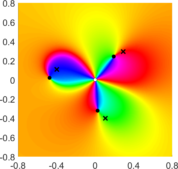
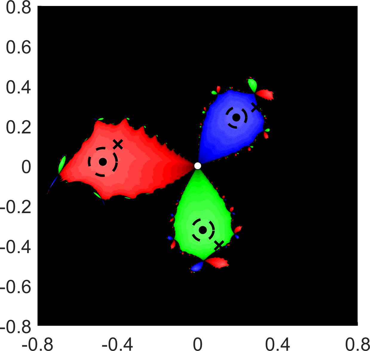
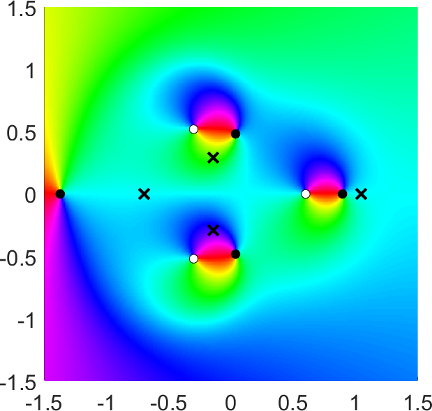
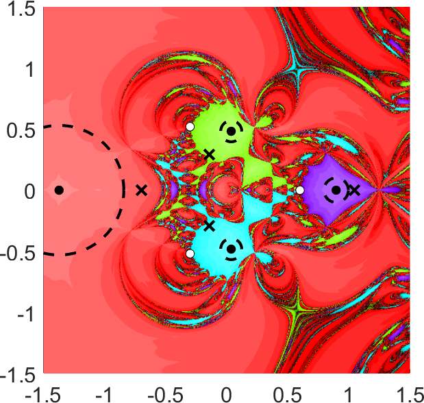
Figure 5: Phase plots (left) and basins of attraction (right) of $f(z)=\frac{1}{z^{3}}+10(1+i)+\overline{\left(\frac{2i}{z^{2}}\right)}$ (top) and $f(z)=\frac{z^{2}}{z^{3}-0.6^{3}}-0.7-\overline{z}$ (bottom) from Example 4.6. Crosses indicate the initial points for the harmonic Newton method from Theorem 4.3 and Corollary 4.5. The dashed circles are regions of convergence guaranteed by Theorem 2.3.

Let $f(z)=\frac{1}{z^{3}}+10(1+i)+\overline{\left(\frac{2i}{z^{2}}\right)}$, where the analytic and anti-analytic part have poles of order $3$ and $2$ in $z_{0}=0$, with $c=-10(1+i)$. As predicted by Theorem 4.3, there are three distinct zeros close to $z_{0}=0$; see Figure 5. The initial points from the theorem (marked by crosses) lie close to the edges of the basins. After $9$ steps of the harmonic Newton iteration, the maximal residual is $3.5527\cdot 10^{-15}$. For points in the black region, the sequence of harmonic Newton iterates tends to $\infty$. Note that the boundary of the basins of attraction seems to have fractal character; compare to the “Douady rabbit”.

Next, we consider the function $f(z)=\frac{z^{2}}{z^{3}-0.6^{3}}-0.7-\overline{z}$, which is the function from Example 2.1 with an additive perturbation. The function has three simple poles, one zero close to each pole, and a fourth zero; see Figure 5. The crosses indicate the initial points from Theorem 4.3 and from Corollary 4.5 (for the fourth zero). As for the previous example, they are close to the boundary of the basins of attraction of the zeros, which again suggests that the constant $c$ cannot be much smaller. After $7$ steps of the harmonic Newton iteration, the maximal residual of the iterates is $4.3299\cdot 10^{-15}$.

The plot of the basins of attraction of the two functions also show dashed circles, which are regions of convergence guaranteed by the refined Newton-Mysovskii theorem (Theorem 2.3). For a zero $z_{*}$ of $f$, this region is computed as follows. Since the theorem guarantees convergence for initial points in a disk, we choose $D$ as a disk with radius $r$ and center $z_{*}$. To estimate the constant $\omega$, we evaluate (2.6) on a grid in $D$. The points in the disk with radius $\min\{r,2/\omega\}$ and center $z_{*}$ are guaranteed to converge to $z_{*}$, and we maximize over $r$ to compute the largest such disk. We observe that our initial points are not covered by Theorem 2.3, but the iterates converge nevertheless to zeros of the functions.

5 Behavior near the critical set

The harmonic Newton map is not defined on the critical set $\mathcal{C}$; see Section 3. Nevertheless, in Examples 4.1 and 6.3 below, the harmonic Newton method approximates singular zeros, i.e., $f(z_{0})=0$ with $z_{0}\in\mathcal{C}$, reasonably well. We now consider solutions of $f(z)=\eta$ with small $\lvert\eta\rvert$ and $z$ close to the singular zero $z_{0}$. For rational harmonic functions $f(z)=r(z)-\overline{z}$, these solutions play a crucial role in the study of the (global) number of zeros of $f$; see [25]. As it turns out, the number of (local) solutions of $f(z)=\eta$ close to $z_{0}$ can be $0,1,2$, or $3$, depending on $\eta$ and $z_{0}$.

Let $f$ be a general harmonic mapping with a singular zero $z_{0}$. We prove existence of solutions of the equation $f(z)=\eta$ by showing convergence of the harmonic Newton iteration with suitable initial points to zeros of $f(z)-\eta$. Depending on $\eta$, the shape of the basins of attraction and the number of solutions can change dramatically.

For simplicity we transform $f=h+\overline{g}$ in a local normal form. Let $z_{0}\in\mathcal{C}$ be a singular zero of $f$ with $\lvert h^{\prime}(z_{0})\rvert=\lvert g^{\prime}(z_{0})\rvert\neq 0$; see (2.3). We then have

$$f(z)=h(z)+\overline{g(z)}=\sum_{k=0}^{\infty}a_{k}(z-z_{0})^{k}+\overline{\sum_{k=0}^{\infty}b_{k}(z-z_{0})^{k}}$$

with $0=f(z_{0})=a_{0}+\overline{b_{0}}$, and $0\neq\overline{b_{1}}=a_{1}e^{i2\theta}$, $\theta\in[0,\pi[$. Hence,

$$f(z)=\frac{\overline{b_{1}}}{e^{i\theta}}\left(\sum_{k=1}^{\infty}\frac{a_{k}}{\overline{b_{1}}}e^{i(k+1)\theta}(e^{-i\theta}(z-z_{0}))^{k}+\overline{\sum_{k=1}^{\infty}\frac{b_{k}}{b_{1}}e^{i(k-1)\theta}(e^{-i\theta}(z-z_{0}))^{k}}\right),$$

and substituting

$$\zeta=e^{-i\theta}(z-z_{0}),\quad\alpha_{k}=\frac{a_{k}}{\overline{b_{1}}}e^{i(k+1)\theta}=\frac{a_{k}}{a_{1}}e^{i(k-1)\theta},\quad\beta_{k}=\frac{b_{k}}{b_{1}}e^{i(k-1)\theta},$$ (5.1)

gives $f(z)=\overline{b}_{1}e^{-i\theta}\widetilde{f}(\zeta)$, where $\widetilde{f}$ is the unique local normal form of $f$ at $z_{0}$,

$$\widetilde{f}(\zeta)=\zeta+\overline{\zeta}+\sum_{k=2}^{\infty}\alpha_{k}\zeta^{k}+\overline{\sum_{k=2}^{\infty}\beta_{k}\zeta^{k}}.$$ (5.2)

Here we used translation ($\zeta_{0}=0$), and scaling and rotation ($\alpha_{1}=\beta_{1}=0$).

We take solutions of the truncated problem $\zeta+\overline{\zeta}+\alpha_{2}\zeta^{2}+\overline{\beta}_{2}\overline{\zeta}^{2}=\eta$ that are close to the origin as initial points for the harmonic Newton method applied to $\widetilde{f}(\zeta)-\eta$.

Lemma 5.1

Let $f=h+\overline{g}$ be as in (5.2),

$$f(\zeta)=\zeta+\overline{\zeta}+\sum_{k=2}^{\infty}\alpha_{k}\zeta^{k}+\overline{\sum_{k=2}^{\infty}\beta_{k}\zeta^{k}}.$$

In particular, $f$ has a singular zero at $0$ with $\lvert h^{\prime}(0)\rvert=\lvert g^{\prime}(0)\rvert\neq 0$. Furthermore, let $f_{\delta c}(\zeta)=f(\zeta)-\delta c$ with $c=-(\alpha_{2}+\overline{\beta}_{2})$ and real $\delta\in\mathbb{R}$.

1. For $\operatorname{Im}(c)\neq 0$ and sufficiently small $\delta>0$, the function $f_{\delta c}$ has two distinct zeros close to $0$. These zeros are the limits of the harmonic Newton iteration for $f_{\delta c}$ with the initial points $\zeta_{\pm}=\pm i\sqrt{\delta}$.

2. For $\operatorname{Im}(c)=0$, $\lvert\alpha_{2}\rvert\neq\lvert\beta_{2}\rvert$, and sufficiently small $\lvert\delta\rvert$, the harmonic Newton iteration for $f_{\delta c}$ with initial point $\zeta_{3}=\frac{1-\sqrt{1-\delta c^{2}}}{c}$ converges to a zero of $f_{\delta c}$.

To apply the Newton-Kantorovich theorem to $f_{\delta c}$ and each initial point, we estimate $\alpha$ and $\omega_{0}$; see (4.1) and (4.2).

Let $\operatorname{Im}(c)\neq 0$. Since $\zeta_{\pm}=\pm i\sqrt{\delta}$ solves $\zeta+\overline{\zeta}+\alpha_{2}\zeta^{2}+\overline{\beta}_{2}\overline{\zeta}^{2}=\delta c$, we have

$$\lvert f_{\delta c}(\zeta_{\pm})\rvert\leq(\lvert\alpha_{3}\rvert+\lvert\beta_{3}\rvert)\lvert\zeta_{\pm}\rvert^{3}+\mathcal{O}(\lvert\zeta_{\pm}\rvert^{4}).$$

From

$$h^{\prime}(\zeta)=1+2\alpha_{2}\zeta+\mathcal{O}(\zeta^{2}),\quad g^{\prime}(\zeta)=1+2\beta_{2}\zeta+\mathcal{O}(\zeta^{2}),$$

we have, using $\overline{\zeta}_{\pm}=-\zeta_{\pm}$,

$$\lvert h^{\prime}(\zeta_{\pm})\rvert^{2}=h^{\prime}(\zeta_{\pm})\overline{h^{\prime}(\zeta_{\pm})}=1+4i\operatorname{Im}(\alpha_{2})\zeta_{\pm}+\mathcal{O}(\lvert\zeta_{\pm}\rvert^{2}),$$

and similarly for $g$. Thus

$$\big{\lvert}\lvert h^{\prime}(\zeta_{\pm})\rvert-\lvert g^{\prime}(\zeta_{\pm})\rvert\big{\rvert} =\frac{\big{\lvert}\lvert h^{\prime}(\zeta_{\pm})\rvert^{2}-\lvert g^{\prime}(\zeta_{\pm})\rvert^{2}\big{\rvert}}{\lvert h^{\prime}(\zeta_{\pm})\rvert+\lvert g^{\prime}(\zeta_{\pm})\rvert}=\frac{4\lvert\operatorname{Im}(\alpha_{2}-\beta_{2})\zeta_{\pm}\rvert+\mathcal{O}(\lvert\zeta_{\pm}\rvert^{2})}{2+\mathcal{O}(\lvert\zeta_{\pm}\rvert)}$$

$$=2\lvert\operatorname{Im}(\alpha_{2}-\beta_{2})\rvert\lvert\zeta_{\pm}\rvert+\mathcal{O}(\lvert\zeta_{\pm}\rvert^{2})$$

$$=2\lvert\operatorname{Im}(c)\rvert\lvert\zeta_{\pm}\rvert+\mathcal{O}(\lvert\zeta_{\pm}\rvert^{2}),$$

for sufficiently small $\delta>0$. Together we find

$$\frac{\lvert f_{\delta c}(\zeta_{\pm})\rvert}{\big{\lvert}\lvert h^{\prime}(\zeta_{\pm})\rvert-\lvert g^{\prime}(\zeta_{\pm})\rvert\big{\rvert}} \leq\frac{(\lvert\alpha_{3}\rvert+\lvert\beta_{3}\rvert)\lvert\zeta_{\pm}\rvert^{3}+\mathcal{O}(\lvert\zeta_{\pm}\rvert^{4})}{2\lvert\operatorname{Im}(c)\rvert\lvert\zeta_{\pm}\rvert+\mathcal{O}(\lvert\zeta_{\pm}\rvert^{2})}$$

$$=\frac{\lvert\alpha_{3}\rvert+\lvert\beta_{3}\rvert}{2\lvert\operatorname{Im}(c)\rvert}\lvert\zeta_{\pm}\rvert^{2}+\mathcal{O}(\lvert\zeta_{\pm}\rvert^{3})=\alpha.$$

Next, we estimate $\omega_{0}$ on $D_{\pm}=\{\zeta\in\mathbb{C}:\lvert\zeta-\zeta_{\pm}\rvert<q\lvert\zeta_{\pm}\rvert\}$ for a $0<q<1$. From

$$h^{\prime\prime}(\zeta)=2\alpha_{2}+\mathcal{O}(\zeta),\quad g^{\prime\prime}(\zeta)=2\beta_{2}+\mathcal{O}(\zeta),$$

we have

$$\sup_{\tau\in D_{\pm}}\lvert h^{\prime\prime}(\tau)\rvert+\sup_{\tau\in D_{\pm}}\lvert g^{\prime\prime}(\tau)\rvert\leq 2(\lvert\alpha_{2}\rvert+\lvert\beta_{2}\rvert)+\mathcal{O}(\lvert\zeta_{\pm}\rvert),$$

and

$$\begin{split}\frac{\sup_{\tau\in D_{\pm}}\lvert h^{\prime\prime}(\tau)\rvert+\sup_{\tau\in D_{\pm}}\lvert g^{\prime\prime}(\tau)\rvert}{\big{\lvert}\lvert h^{\prime}(\zeta_{\pm})\rvert-\lvert g^{\prime}(\zeta_{\pm})\rvert\big{\rvert}}&\leq\frac{2(\lvert\alpha_{2}\rvert+\lvert\beta_{2}\rvert)+\mathcal{O}(\lvert\zeta_{\pm}\rvert)}{2\lvert\operatorname{Im}(c)\rvert\lvert\zeta_{\pm}\rvert+\mathcal{O}(\lvert\zeta_{\pm}\rvert^{2})}\\ &=\frac{\lvert\alpha_{2}\rvert+\lvert\beta_{2}\rvert}{\lvert\operatorname{Im}(c)\rvert\lvert\zeta_{\pm}\rvert}+\mathcal{O}(1)=\omega_{0}.\end{split}$$

Thus

$$h_{0}=\alpha\omega_{0}=\frac{(\lvert\alpha_{2}\rvert+\lvert\beta_{2}\rvert)(\lvert\alpha_{3}\rvert+\lvert\beta_{3}\rvert)}{2\lvert\operatorname{Im}(c)\rvert^{2}}\lvert\zeta_{\pm}\rvert+\mathcal{O}(\lvert\zeta_{\pm}\rvert^{2}),$$

so that $h_{0}<\frac{1}{2}$ for sufficiently small $\delta$, since $\zeta_{\pm}=\pm i\sqrt{\delta}\to 0$ for $\delta\to 0$. Finally, we show $\rho<q\lvert\zeta_{\pm}\rvert$. Using (2.7) we find that

$$\rho=\alpha+\mathcal{O}(\alpha h_{0})=\frac{\lvert\alpha_{3}\rvert+\lvert\beta_{3}\rvert}{2\lvert\operatorname{Im}(c)\rvert}\lvert\zeta_{\pm}\rvert^{2}+\mathcal{O}(\lvert\zeta_{\pm}\rvert^{3})<q\lvert\zeta_{\pm}\rvert,$$ (5.3)

provided $\zeta_{\pm}$ is sufficiently small. Then, by Theorem 2.2, the sequence of harmonic Newton iterates remains in the closed disks $\overline{D}(\zeta_{\pm};\rho)$ and converges to a zero of $f_{\delta c}$. Furthermore, both disks are disjoint, which implies that the iterations converge to two distinct zeros of $f_{\delta c}$.

For the second part, assume that $\operatorname{Im}(c)=0$ and $\lvert\alpha_{2}\rvert\neq\lvert\beta_{2}\rvert$. The latter implies that $c\neq 0$. The only difference to the first case is in the estimate of $\big{\lvert}\lvert h^{\prime}(\zeta_{3})\rvert-\lvert g^{\prime}(\zeta_{3})\rvert\big{\rvert}$. Since $c$ is real, also $\zeta_{3}=\frac{1-\sqrt{1-\delta c^{2}}}{c}=\frac{c}{2}\delta+\mathcal{O}(\delta^{2})$ is real for $\delta\leq\frac{1}{c^{2}}$, and we find from $h^{\prime}(\zeta)=1+2\alpha_{2}\zeta+\mathcal{O}(\zeta^{2})$ that

$$\lvert h^{\prime}(\zeta_{3})\rvert^{2}=h^{\prime}(\zeta_{3})\overline{h^{\prime}(\zeta_{3})}=1+4\operatorname{Re}(\alpha_{2})\zeta_{3}+\mathcal{O}(\lvert\zeta_{3}\rvert^{2}),$$

and similarly for $g$. Then

$$\big{\lvert}\lvert h^{\prime}(\zeta_{3})\rvert-\lvert g^{\prime}(\zeta_{3})\rvert\big{\rvert} =\frac{\big{\lvert}\lvert h^{\prime}(\zeta_{3})\rvert^{2}-\lvert g^{\prime}(\zeta_{3})\rvert^{2}\big{\rvert}}{\lvert h^{\prime}(\zeta_{3})\rvert+\lvert g^{\prime}(\zeta_{3})\rvert}=\frac{\lvert 4\operatorname{Re}(\alpha_{2}-\beta_{2})\zeta_{3}+\mathcal{O}(\zeta_{3}^{2})\rvert}{2+\mathcal{O}(\lvert\zeta_{3}\rvert)}$$

$$=2\lvert\operatorname{Re}(\alpha_{2}-\beta_{2})\rvert\lvert\zeta_{3}\rvert+\mathcal{O}(\lvert\zeta_{3}\rvert^{2}).$$

The assumptions $\lvert\alpha_{2}\rvert\neq\lvert\beta_{2}\rvert$ and $\operatorname{Im}(c)=0$ guarantee that $\operatorname{Re}(\alpha_{2}-\beta_{2})\neq 0$ and thus that $\big{\lvert}\lvert h^{\prime}(\zeta_{3})\rvert-\lvert g^{\prime}(\zeta_{3})\rvert\big{\rvert}=\mathcal{O}(\lvert\zeta_{3}\rvert)$. We then obtain $\alpha$, $\omega_{0}$ in the same orders of magnitude as in the first case, so that $h_{0}=\alpha\omega_{0}=\mathcal{O}(\lvert\zeta_{3}\rvert)<\frac{1}{2}$ and $\rho<q\lvert\zeta_{3}\rvert$ for sufficiently small $\lvert\delta\rvert$. Therefore, the harmonic Newton iteration with initial point $\zeta_{3}$ converges to a zero of $f_{\delta c}$.

Theorem 5.2

Let the harmonic mapping

$$f(z)=h(z)+\overline{g(z)}=\sum_{k=1}^{\infty}a_{k}(z-z_{0})^{k}+\overline{\sum_{k=1}^{\infty}b_{k}(z-z_{0})^{k}}$$

have a singular zero at $z_{0}$ with $\lvert a_{1}\rvert=\lvert b_{1}\rvert\neq 0$. Furthermore, let $\theta\in[0,\pi[$ be defined by $\overline{b}_{1}=a_{1}e^{i2\theta}$, and let

$$f_{\delta c}(z)=f(z)-\delta c,\quad\text{with}\quad c=\overline{b}_{1}e^{-i\theta}\widetilde{c}\quad\text{and}\quad\widetilde{c}=-\frac{a_{2}}{a_{1}}e^{i\theta}-\overline{\left(\frac{b_{2}}{b_{1}}e^{i\theta}\right)},$$

where $\delta$ is real.

1. For $\operatorname{Im}(\widetilde{c})\neq 0$ and sufficiently small $\delta>0$, the function $f_{\delta c}$ has two distinct zeros close to $z_{0}$. These zeros are the limits of the harmonic Newton iteration for $f_{\delta c}$ with the initial points

   $$z_{\pm}=z_{0}\pm i\sqrt{\delta}e^{i\theta}=z_{0}\pm i\sqrt{\delta\frac{\overline{b}_{1}}{a_{1}}}.$$

2. For $\operatorname{Im}(\widetilde{c})=0$, $\lvert a_{2}\rvert\neq\lvert b_{2}\rvert$, and sufficiently small $\lvert\delta\rvert$, the harmonic Newton iteration with initial point

   $$z_{3}=z_{0}+\frac{1-\sqrt{1-\delta\widetilde{c}^{2}}}{\widetilde{c}}e^{i\theta},$$

   converges to a zero of $f_{\delta c}$.

We transform $f$ to its local normal form $\widetilde{f}$ at $z_{0}$, recall (5.1), (5.2), and $f(z)=\overline{b}_{1}e^{-i\theta}\widetilde{f}(\zeta)$. Then $f(z)-\delta c=\overline{b}_{1}e^{-i\theta}(\widetilde{f}(\zeta)-\delta\widetilde{c})$ with

$$\widetilde{c}=-\frac{a_{2}}{a_{1}}e^{i\theta}-\overline{\left(\frac{b_{2}}{b_{1}}e^{i\theta}\right)}=-(\alpha_{2}+\overline{\beta}_{2}).$$

Let $\operatorname{Im}(\widetilde{c})\neq 0$. Then, by Lemma 5.1, the harmonic Newton iteration with initial points $\zeta_{\pm}=\pm i\sqrt{\delta}$ converges to zeros of $\widetilde{f}_{\delta\widetilde{c}}$, when $\delta>0$ is sufficiently small. Back transformation gives the desired result; see (5.1).

Let $\operatorname{Im}(\widetilde{c})=0$, and $\lvert\alpha_{2}\rvert\neq\lvert\beta_{2}\rvert$, which is equivalent to $\lvert a_{2}\rvert\neq\lvert b_{2}\rvert$. Then, by Lemma 5.1, the harmonic Newton iteration with initial point $\zeta_{3}=\frac{1-\sqrt{1-\delta\widetilde{c}^{2}}}{\widetilde{c}}$ converges to a zero of $\widetilde{f}_{\delta\widetilde{c}}$, when $\delta>0$ is sufficiently small. Back transformation gives the desired result.

Varying $\delta$ can lead to a bifurcation of the solutions of $f(z)=\delta c$, and the basins of attraction can merge or split; see Figure 6.

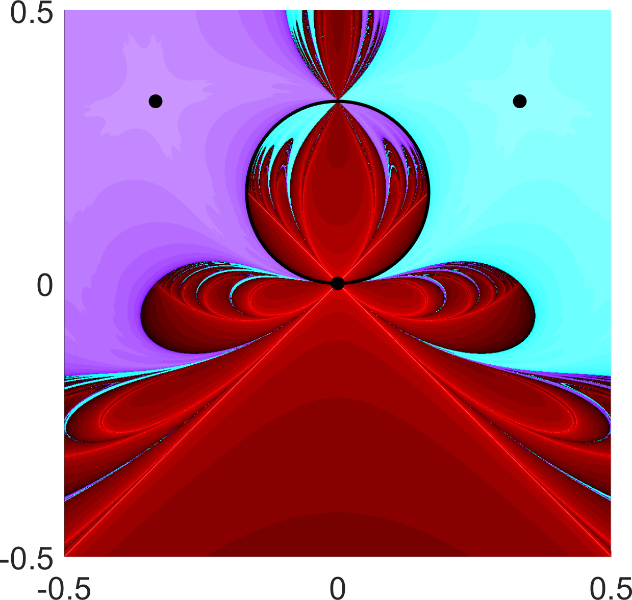
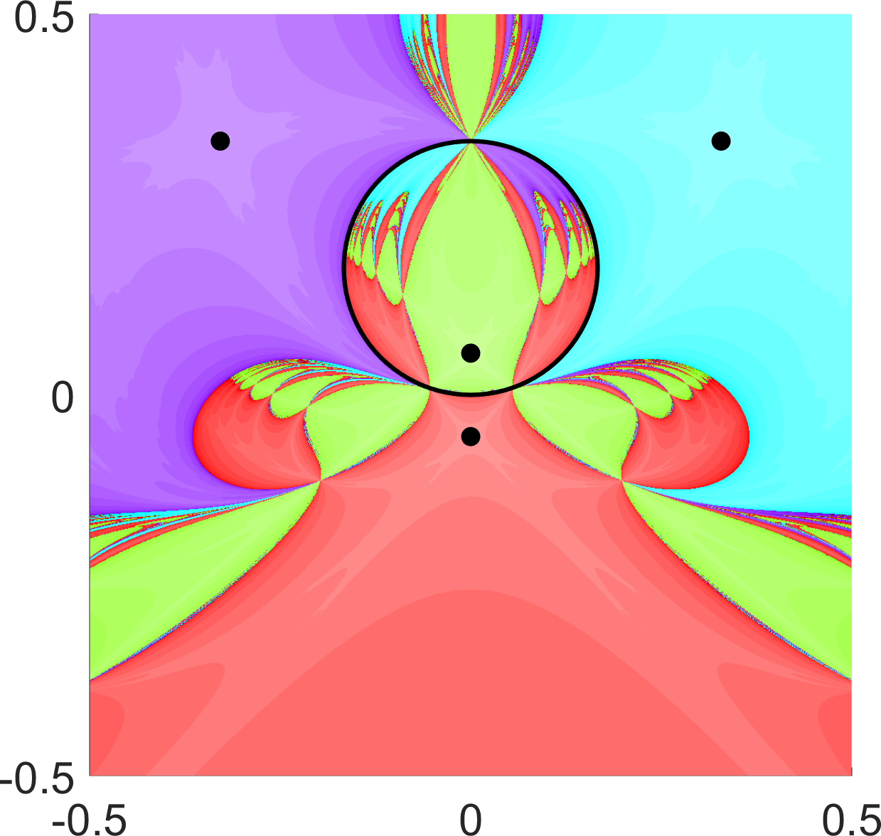
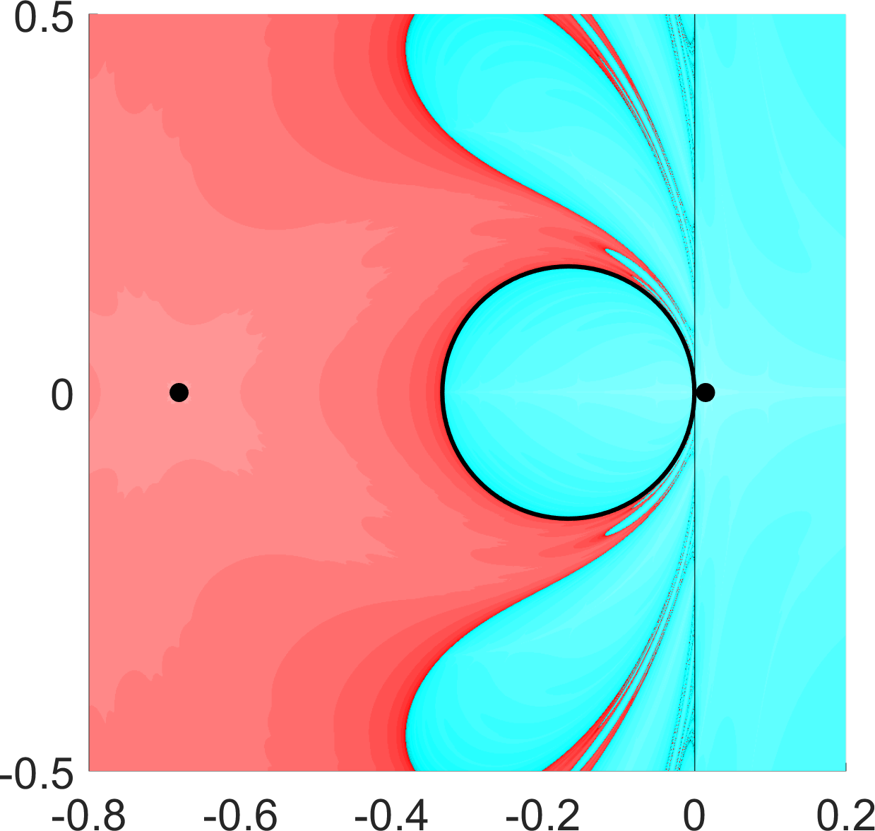
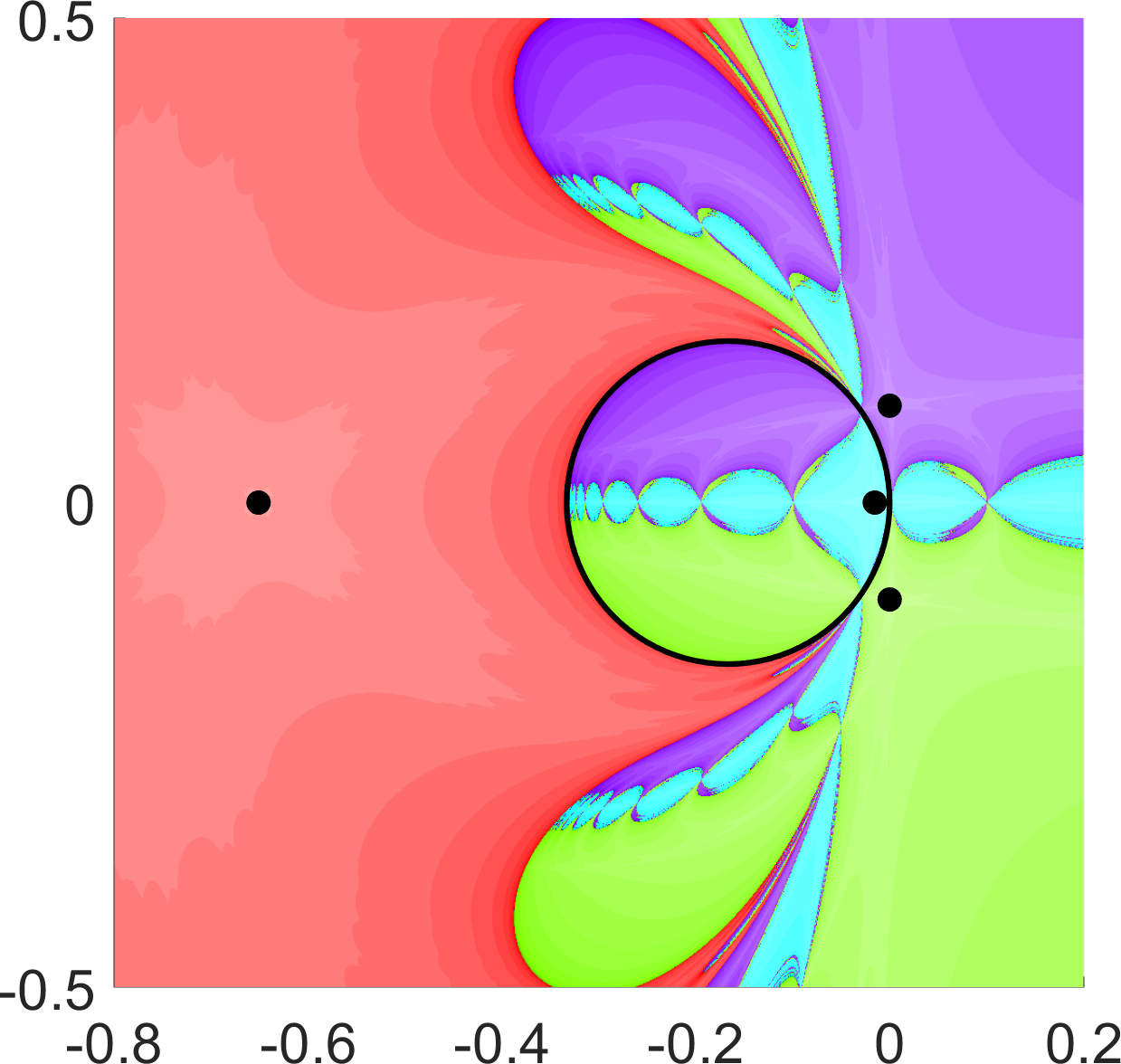
Figure 6: Basins of attraction. Top: $f_{-i\delta}(z)=z+\overline{z}+2iz^{2}+\overline{iz^{2}}+i\delta$ with $\delta=0$ (left) and $\delta=0.003$ (right). Bottom: $f_{-3\delta}(z)=z+\overline{z}+2z^{2}+\overline{z}^{2}+3\delta$ with $\delta=-0.01$ (left) and $\delta=0.01$ (right). Black lines mark the critical sets.

Remark 5.3

1. The conditions $\operatorname{Im}(c)\neq 0$ in Lemma 5.1 and $\operatorname{Im}(\widetilde{c})\neq 0$ in Theorem 5.2 imply that $f(z_{0})$ is not a cusp of the caustics of $f$; see [25].

2. In Figure 6, the singular zero at $z=0$ (top left) splits into two non-singular zeros (top right). Note that the harmonic Newton iteration converges quicker to the non-singular zeros than to the singular zero.

3. For $f$ in Figure 6 (bottom left) we have $H_{f}(iy)=\frac{i}{2}(y-\frac{0.01}{y})$, $y\in\mathbb{R}$. Hence, the harmonic Newton iteration diverges for initial points on the imaginary axis, which explains the black line.

4. Figure 6 (bottom right) suggests that we have zeros of $f_{\delta c}$ close to $z_{\pm}=\pm i\sqrt{\delta}$ also in the case $\operatorname{Im}(c)=0$ and $\delta>0$. However, without further improvements, the above proof strategy breaks down for $z_{\pm}$ as initial points.

6 Further Examples

We illustrate the harmonic Newton method with further examples, using the MATLAB implementation in Figure 3.

6.1 Harmonic polynomials

Harmonic polynomials are of the form $f=p+\overline{q}$, where $p$ and $q$ are (analytic) polynomials with respective degrees $n$ and $m$. Wilmshurst conjectured in [45] that the number of zeros of $f$ for $n>m$ fulfills

$$N(f)\leq 3n-2+m(m-1),$$ (6.1)

and proved it for $m=n-1$, including sharpness of the bound. For $n=m$, Wilmshurst showed the bound $N(f)\leq n^{2}$, provided that $\lim_{z\to\infty}f(z)=\infty$ holds. Otherwise $f$ could have infinitely many zeros; compare Lemma 4.2. Later, the case $m=1$ was settled in [23], and sharpness of the bound in [13]. For several other values of $1<m<n-1$, the conjecture was shown to be wrong; see [24, 15, 19].

Example 6.1

We consider the original example of Wilmshurst in [45] showing sharpness of (6.1) for $m=n-1$. Let

$$f(z)=p(z)+\overline{q(z)}=z^{n}+(z-1)^{n}+\overline{i(z-1)^{n}-iz^{n}},$$ (6.2)

which has $\deg(p)=n$, and $\deg(q)=n-1$, and $n^{2}$ zeros.

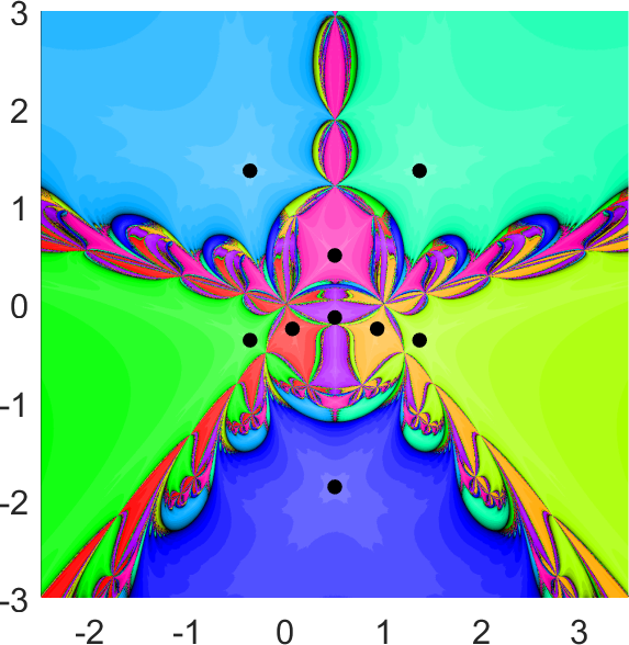
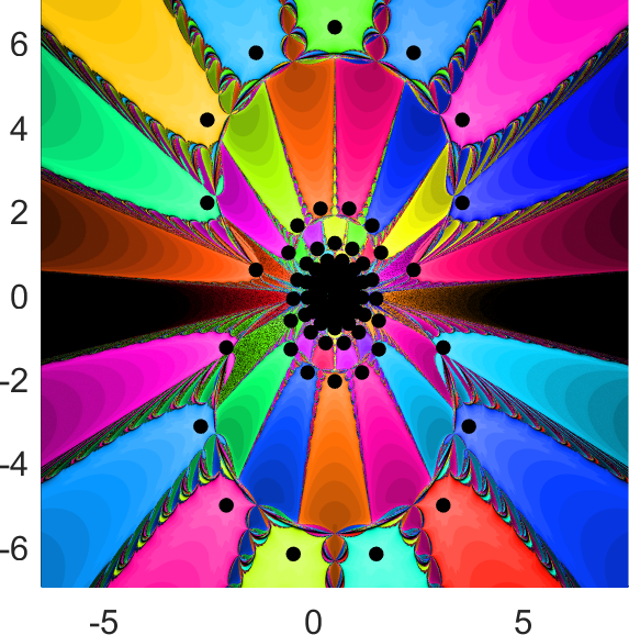
Figure 7: Phase plots (left) and basins of attraction (right) for Wilmshurst’s harmonic polynomial (6.2) for $n=3$ (top) and $n=10$ (bottom).

To compute the zeros of $f$ with the harmonic Newton method, we use a grid of initial points with mesh size $0.05$ in the plot region in Figure 7. On the left we have the phase plots, and on the right the basins of attraction for $n=3$ and the $n^{2}=9$ zeros (top), as well as for $n=10$ with its $100$ zeros (bottom). The plots are centered at $z=0.5$, since $z\mapsto p(z+0.5)$ and $z\mapsto q(z+0.5)$ are even or odd, depending on $n$.

For $n=3$, the maximal residual of $f$ at the computed zeros is $9.8625\cdot 10^{-15}$. For $n=10$, we have $\lvert f(z_{j})\rvert\leq 3.0146\cdot 10^{-14}$ at computed zeros with $\lvert z_{j}-0.5\rvert\leq 1$, and $\lvert f(z_{j})\rvert\leq 1.3738\cdot 10^{-7}$ at zeros with $\lvert z_{j}-0.5\rvert>1$. The latter rather large absolute residual is an effect of floating point arithmetic. Indeed, the magnitude of $z^{n}$ and $(z-1)^{n}$ is of order $10^{8}$ at the outer zeros, which results in a loss of accuracy of about $8$ digits when evaluating $f$. Evaluating the polynomials $p$ and $q$ with Horner’s scheme [17, Sect. 5.1] does not alleviate this problem, since we still need to compute $p+\overline{q}$. However, the maximum of the relative residuals $\lvert f(z_{j})\rvert/\lvert z_{j}-0.5\rvert^{10}$ is $1.4010\cdot 10^{-14}$, which is quite satisfactory.

6.2 Gravitational lensing

Gravitational lensing can be modeled with harmonic mappings, where positions of lensed images are zeros of these functions; see [22, 34, 3]. We consider point mass lenses and isothermal gravitational lenses.

Example 2.1 already featured a rational harmonic function from gravitational point mass models. Rhie [36] constructed from this example a gravitational lens with the maximum number of lensed images, or equivalently a rational harmonic function with the maximum number of zeros, showing sharpness of the bound in [21].

Example 6.2

Rhie’s function

$$f(z)=(1-\varepsilon)\frac{z^{n-1}}{z^{n}-r^{n}}+\frac{\varepsilon}{z}-\overline{z}$$ (6.3)

is obtained from (2.4) by adding a pole at the origin (and normalizing the mass to be one).

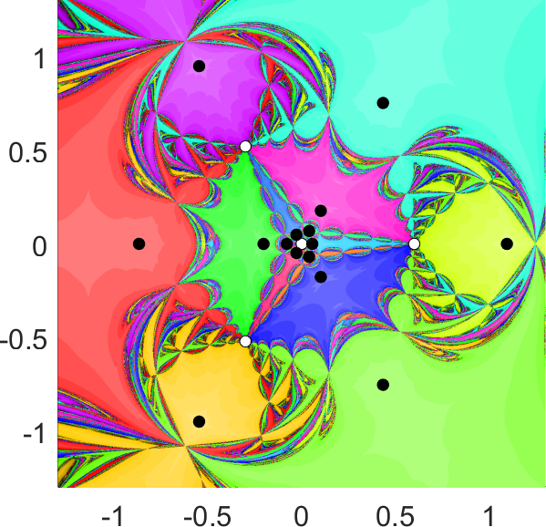
Figure 8: Phase plot (left) and basins of attraction (right) for Rhie’s function (6.3) with $r=0.6$, $n=3$, and $\varepsilon=0.004$; compare Figure 2.

For sufficiently small $\varepsilon$, it has $5n$ zeros; for a rigorous proof and quantification of the parameters $\varepsilon$ and $r$ see [28]. To compute the zeros of $f$ with $n=3$, $r=0.6$ and $\varepsilon=0.004$, we apply the harmonic Newton method to a grid of initial points (mesh size $0.05$); see Figure 8. The maximal residual at the computed zeros is $9.9371\cdot 10^{-15}$.

Example 6.3

A point mass lens with a single mass is known as the Chang-Refsdal lens and produces an Einstein ring; see [2]. It can be modeled by $f(z)=\frac{1}{z}-\overline{z}$. The zero set of $f$ is the whole unit circle, in particular the zeros are not isolated. Moreover, each zero is singular.

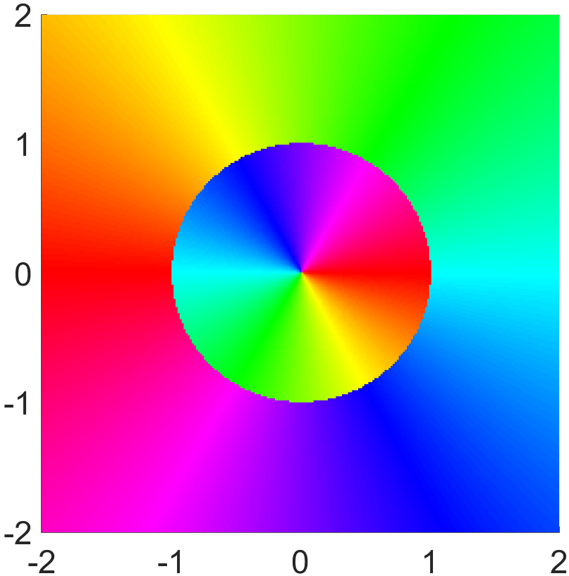
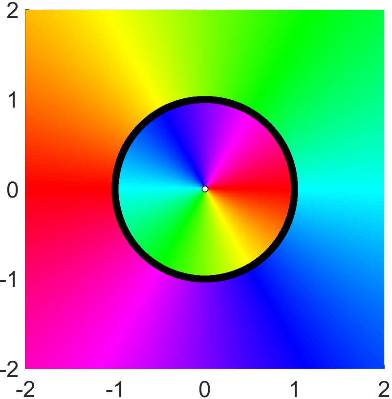
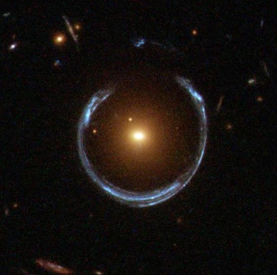
Figure 9: Phase plots of $f(z)=1/z-\overline{z}$. The middle panel shows the computed zeros of $f$; see Example 6.3. The right panel shows an actual gravitional lens (image credit: ESA/Hubble & NASA).

To compute zeros of $f$, we take a grid of initial points in $[-2,2]^{2}$ (mesh size $0.02$). Figure 9 shows the iterates after at most $30$ steps (the mean number of steps is $6.4$). The residuals satisfy $\lvert f(z_{k})\rvert\leq 2.4887\cdot 10^{-14}$. The harmonic Newton iteration for $f$ simplifies to $z_{k+1}=\frac{2}{1+\lvert z_{k}\rvert^{2}}z_{k}$ for $\lvert z_{k}\rvert\neq 1$, showing that $z_{k}\to e^{i\varphi}$ if $z_{0}=r_{0}e^{i\varphi}\neq 0$, i.e., the basin of attraction of $e^{i\varphi}$ is

$$A(e^{i\varphi})=\{z=re^{i\varphi}:r>0,r\neq 1\}.$$

Note that $A(e^{i\varphi})$ does not contain an open subset around $e^{i\varphi}$, which is due to the fact that the zeros of $f$ are not isolated.

Example 6.4

We consider gravitational lensing by an isothermal elliptical galaxy with compactly supported mass; see [3, 20, 4]. After a change of variables, the lensed images are the zeros of the transcendental harmonic mapping

$$f(z)=z-\arcsin\left(\frac{k}{\overline{z}+\overline{w}}\right),$$ (6.4)

where $w$ is the position of the light source (projected onto the lens plane), and $k$ is a real constant related to the shape of the galaxy; see [20]. We take the principal branch of arcsine

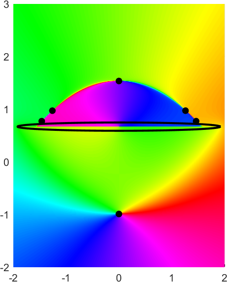
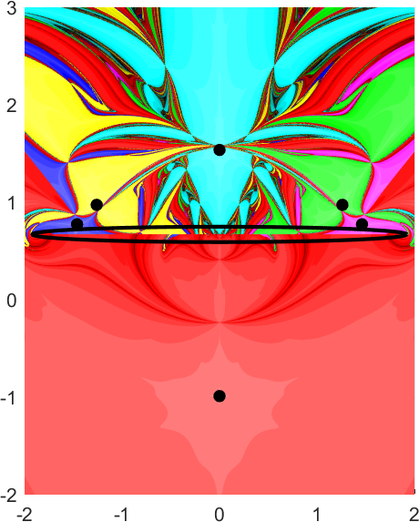
Figure 10: Phase plot (left) and basins of attraction (right) for the function $f(z)=z-\arcsin(1.92/\overline{z-0.67i})$ in Example 6.4; compare to [20, Fig. 3].

and compute the zeros of $f$ by applying the harmonic Newton method to a grid of initial points in $[-2,2]^{2}$ (mesh size $0.02$). Figure 10 shows the phase plot of $f$ (left) and the basins of attraction (right) for $k=1.92$ and $w=-0.67i$ from [4]. The black ellipse is the shape of the galaxy, and the sharp edge in the phase plot (inside the ellipse) is the branch cut of arcsine.

7 Summary and Outlook

We derived a complex formulation of Newton’s method for harmonic mappings and, more generally, for real differentiable functions in $\mathbb{C}$. The iterations (3.3) and its harmonic pendant (3.6) allow to compute the zeros of harmonic and even non-analytic complex functions without losing any advantages of Newton’s method. The complex formulation makes the iteration amenable to analysis in a complex variables spirit. In particular, close to a pole of a harmonic mapping $f$, we derived initial points for which the harmonic Newton iteration is guaranteed to converge to zeros of $f$. Similarly, we derived initial points to obtain solutions of $f(z)=\eta$ for certain small $\lvert\eta\rvert$ and $z$ close to a singular zero of $f$. In both cases, the convergence proof relies on the Newton-Kantorovich theorem. In particular, our theorems also show existence of zeros.

The harmonic Newton method should prove useful in the further study of harmonic polynomials, in particular related to Wilmshurst’s conjecture, and more generally of harmonic mappings. Visualizing the basins of attraction can give new insights into the behavior of the functions.

For certain classes of harmonic mappings, e.g., harmonic polynomials, it could be interesting to find a set $\mathcal{S}$, such that for any zero $z_{*}$ of $f$, the harmonic Newton iteration converges to $z_{*}$ for at least one initial point in $\mathcal{S}$. This approach is related to Theorem 4.3 and Theorem 5.2. In the seminal paper [18], such a set $\mathcal{S}$ is constructed for complex (analytic) polynomials.

A further analysis of the harmonic Newton map $H_{f}$ in the spirit of complex dynamics should be of great interest, e.g., points of indeterminacy, and the continuation of $H_{f}$ (and of $f$ itself) to the Riemann sphere. Both have not been addressed in this paper.

For analytic functions, many other iterative root finding methods exist; see e.g. [14, 42]. It could be interesting to generalize them to harmonic mappings. As a drawback we may have to introduce higher order derivatives for harmonic mappings. The efficiency index of several of these methods for analytic functions are compared in [42]. In this light, Newton’s method should be a decent choice.

Acknowledgments.

We thank Jörg Liesen for helpful comments on the manuscript. Moreover, we thank the anonymous referees for several helpful suggestions which lead to improvements of the presentation.

References

- [1] M. J. Ablowitz and A. S. Fokas, Complex variables: introduction and applications, Cambridge Texts in Applied Mathematics, Cambridge University Press, Cambridge, second ed., 2003.
- [2] J. H. An and N. W. Evans, The Chang–Refsdal lens revisited, Monthly Notices Roy. Astronom. Soc., 369 (2006), pp. 317–334.
- [3] C. Bénéteau and N. Hudson, A survey on the maximal number of solutions of equations related to gravitational lensing, in Complex analysis and dynamical systems, Trends Math., Birkhäuser/Springer, Cham, 2018, pp. 23–38.
- [4] W. Bergweiler and A. Eremenko, On the number of solutions of a transcendental equation arising in the theory of gravitational lensing, Comput. Methods Funct. Theory, 10 (2010), pp. 303–324.
- [5] D. Bshouty and A. Lyzzaik, Problems and conjectures in planar harmonic mappings, J. Anal., 18 (2010), pp. 69–81.
- [6] L. Carleson and T. W. Gamelin, Complex dynamics, Universitext: Tracts in Mathematics, Springer-Verlag, New York, 1993.
- [7] J. Clunie and T. Sheil-Small, Harmonic univalent functions, Ann. Acad. Sci. Fenn. Ser. A I Math., 9 (1984), pp. 3–25.
- [8] R. De Leo, “Simple Dynamics” conjectures for some real Newton maps on the plane, ArXiv e-prints: 1812.00270, (2018).
- [9] , Julia sets of Newton maps of real quadratic polynomial maps on the plane, ArXiv e-prints: 1812.11595, (2019).
- [10] P. Deuflhard, Newton methods for nonlinear problems, vol. 35 of Springer Series in Computational Mathematics, Springer, Heidelberg, 2011.
- [11] P. Duren, Harmonic mappings in the plane, vol. 156 of Cambridge Tracts in Mathematics, Cambridge University Press, Cambridge, 2004.
- [12] P. Duren, W. Hengartner, and R. S. Laugesen, The argument principle for harmonic functions, Amer. Math. Monthly, 103 (1996), pp. 411–415.
- [13] L. Geyer, Sharp bounds for the valence of certain harmonic polynomials, Proc. Amer. Math. Soc., 136 (2008), pp. 549–555.
- [14] W. J. Gilbert, Generalizations of Newton’s method, Fractals, 9 (2001), pp. 251–262.
- [15] J. D. Hauenstein, A. Lerario, E. Lundberg, and D. Mehta, Experiments on the zeros of harmonic polynomials using certified counting, Exp. Math., 24 (2015), pp. 133–141.
- [16] P. Henrici, Applied and computational complex analysis. Vol. 3, John Wiley & Sons, Inc., New York, 1986.
- [17] N. J. Higham, Accuracy and stability of numerical algorithms, Society for Industrial and Applied Mathematics (SIAM), Philadelphia, PA, second ed., 2002.
- [18] J. Hubbard, D. Schleicher, and S. Sutherland, How to find all roots of complex polynomials by Newton’s method, Invent. Math., 146 (2001), pp. 1–33.
- [19] D. Khavinson, S.-Y. Lee, and A. Saez, Zeros of harmonic polynomials, critical lemniscates, and caustics, Complex Anal. Synerg., 4 (2018), pp. 1–20.
- [20] D. Khavinson and E. Lundberg, Transcendental harmonic mappings and gravitational lensing by isothermal galaxies, Complex Anal. Oper. Theory, 4 (2010), pp. 515–524.
- [21] D. Khavinson and G. Neumann, On the number of zeros of certain rational harmonic functions, Proc. Amer. Math. Soc., 134 (2006), pp. 1077–1085.
- [22] , From the fundamental theorem of algebra to astrophysics: a “harmonious” path, Notices Amer. Math. Soc., 55 (2008), pp. 666–675.
- [23] D. Khavinson and G. Świa̧tek, On the number of zeros of certain harmonic polynomials, Proc. Amer. Math. Soc., 131 (2003), pp. 409–414.
- [24] S.-Y. Lee, A. Lerario, and E. Lundberg, Remarks on Wilmshurst’s theorem, Indiana Univ. Math. J., 64 (2015), pp. 1153–1167.
- [25] J. Liesen and J. Zur, How constant shifts affect the zeros of certain rational harmonic functions, Comput. Methods Funct. Theory, 18 (2018), pp. 583–607.
- [26] , The maximum number of zeros of revisited, Comput. Methods Funct. Theory, 18 (2018), pp. 463–472.
- [27] R. Luce and O. Sète, The index of singular zeros of harmonic mappings of anti-analytic degree one, Oberwolfach Report OWP 2017-03, (2017).
- [28] R. Luce, O. Sète, and J. Liesen, Sharp parameter bounds for certain maximal point lenses, Gen. Relativity Gravitation, 46 (2014), pp. 1–16.
- [29] , A note on the maximum number of zeros of , Comput. Methods Funct. Theory, 15 (2015), pp. 439–448.
- [30] J. Milnor, Dynamics in one complex variable, vol. 160 of Annals of Mathematics Studies, Princeton University Press, Princeton, NJ, third ed., 2006.
- [31] S. Mukherjee, S. Nakane, and D. Schleicher, On multicorns and unicorns II: bifurcations in spaces of antiholomorphic polynomials, Ergodic Theory Dynam. Systems, 37 (2017), pp. 859–899.
- [32] S. Nakane and D. Schleicher, On multicorns and unicorns. I. Antiholomorphic dynamics, hyperbolic components and real cubic polynomials, Internat. J. Bifur. Chaos Appl. Sci. Engrg., 13 (2003), pp. 2825–2844.
- [33] H.-O. Peitgen and P. H. Richter, The beauty of fractals. Images of complex dynamical systems, Springer-Verlag, Berlin, 1986.
- [34] A. O. Petters, Gravity’s action on light, Notices Amer. Math. Soc., 57 (2010), pp. 1392–1409.
- [35] R. Remmert, Theory of complex functions, vol. 122 of Graduate Texts in Mathematics, Springer-Verlag, New York, 1991.
- [36] S. H. Rhie, n-point gravitational lenses with 5(n-1) images, ArXiv Astrophysics e-prints: 0305166, (2003).
- [37] O. Sète, R. Luce, and J. Liesen, Creating images by adding masses to gravitational point lenses, Gen. Relativity Gravitation, 47 (2015), pp. 1–8.
- [38] , Perturbing rational harmonic functions by poles, Comput. Methods Funct. Theory, 15 (2015), pp. 9–35.
- [39] S. Smale, Newton’s method estimates from data at one point, in The merging of disciplines: new directions in pure, applied, and computational mathematics (Laramie, Wyo., 1985), Springer, New York, 1986, pp. 185–196.
- [40] T. J. Suffridge and J. W. Thompson, Local behavior of harmonic mappings, Complex Variables Theory Appl., 41 (2000), pp. 63–80.
- [41] L. N. Trefethen and J. A. C. Weideman, The exponentially convergent trapezoidal rule, SIAM Rev., 56 (2014), pp. 385–458.
- [42] J. L. Varona, Graphic and numerical comparison between iterative methods., Math. Intell., 24 (2002), pp. 37–46.
- [43] X. Wang, Convergence of Newton’s method and inverse function theorem in Banach space, Math. Comp., 68 (1999), pp. 169–186.
- [44] E. Wegert, Visual complex functions. An introduction with phase portraits., Birkhäuser/Springer Basel AG, Basel, 2012.
- [45] A. S. Wilmshurst, The valence of harmonic polynomials, Proc. Amer. Math. Soc., 126 (1998), pp. 2077–2081.
- [46] E. Zeidler, Nonlinear functional analysis and its applications. I: Fixed-point theorems, Springer-Verlag, New York, 1986.