First-order solitons with internal structures in an extended Maxwell-$CP(2)$ model

Abstract

We study a Maxwell-$CP(2)$ model coupled to a real scalar field through a dielectric function multiplying the Maxwell term. In such a context, we look for first-order rotationally symmetric solitons by means of the Bogomol’nyi algorithm, i.e. by minimizing the total energy of the effective model. We perform our investigation by choosing an explicit form of the dielectric function. The numerical solutions show regular vortices whose shapes dramatically differ from their canonical counterparts. We can understood such differences as characterizing the existence of an internal structure.

I Introduction

In the context of classical models, topological solitons are commonly described as time-independent solutions inherent to highly nonlinear field theories n5 . For example, in (2+1)-dimensional gauge theories, vortices stand for the rotationally symmetric solutions arising from the Euler-Lagrange equations n1 . In addition, under special circumstances, topological vortices can also be obtained via a particular set of first-order differential equations (instead of the second-order Euler-Lagrange ones). In general, such a first-order framework can be found via a minimization procedure of the total energy of the system, which allows to get a well-defined lower bound for the energy itself n41 -n4 . In this sense, first-order vortices were already verified to occur not only in the usual Maxwell-Higgs scenario n4 , but also in the Chern-Simons cshv and in the composite Maxwell-Chern-Simons-Higgs one n42 .

The study of the first-order solitons arising from a $CP(N-1)$ model is particularly important due to its straight phenomenological connection with the Yang-Mills model defined in four dimensions, as explained in cpn-1 . Under such a perspective, the existence of first-order vortices in a gauged $CP(2)$ scenario endowed with the usual Maxwell’s action was firstly suggested in loginov , being explicitly demonstrated in casana . Moreover, electrically charged first-order vortices were also verified to occur in a gauged $CP(2)$ model in the presence of both the Chern-Simons vini and the composite Maxwell-Chern-Simons actions neyver , separately.

At the same time, in the context of extended field models, it is interesting to point out that the standard Maxwell-Higgs one was itself enlarged in order to accommodate an additional $SO(3)$ spin group (therefore giving rise to spin vortices), the corresponding $SO(3)$ symmetry being driven by an extra scalar sector, see the Ref. witten ; n43 . In view of those results, Bazeia et al. have recently demonstrated that such an enlarged Maxwell-Higgs system supports the existence of well-behaved first-order vortices with internal structures n44 , whilst arguing that such solutions may find important applications in the context of metamaterials n45 .

We now go a little bit further into such a subject by studying the occurrence of first-order rotationally symmetric solitons with internal structures in a gauged $CP(2)$ model containing an additional scalar field. We have implemented successfully the Bogomol’nyi prescription by obtaining an energy lower-bound (Bogomol’nyi limit) and the respective BPS equations satisfied by the fields saturating that bound. We then solve these equations by means of a finite-difference scheme, via which we obtain regular vortices with finite energy. The point to be raised here is that the resulting configurations differ from their canonical counterparts (obtained in the absence of the additional field), these differences being understood as internal structures, as we clarify below.

In order to present our results, this work is organized as follows: in the Sec. II, we introduce the extended model in which the complex $CP(2)$ field couples minimally to the Maxwell term and also interacts with an additional noncharged real scalar field. This additional field also composes the dielectric function multiplying the Maxwell term and the potential of the new model. We focus our attention on those time-independent solitons with rotational symmetry. In this context, we proceed the minimization of the effective energy, from which we obtain a set of three first-order differential equations and a well-defined lower bound for the total energy. In addition, in the Sec. III, we split our investigation into two different cases based on different choices for the dielectric function. In the sequel, we solve the corresponding first-order equations numerically, the resulting profiles dramatically differing from the canonical ones (obtained in the absence of the additional field). We point out such differences can be understood as the so-called internal structures. In the Sec. IV, we end our work by presenting our final comments and perspectives regarding future investigations.

In this work, we use the natural units system, for the sake of simplicity.

II The model

We begin our manuscript by introducing the Lagrange density which defines the (2+1)-dimensional field model under investigation, i.e.

$$\mathcal{L} = -\frac{1}{4}G(\chi)F_{\mu\nu}F^{\mu\nu}+\left(P_{ab}D_{\mu}\phi_{b}\right)^{\ast}P_{ac}D^{\mu}\phi_{c}$$ (1)

$$+\frac{1}{2}\partial_{\mu}\chi\partial^{\mu}\chi-V(\chi,\left|\phi_{3}\right|)\text{,}$$

where $F_{\mu\nu}=\partial_{\mu}A_{\nu}-\partial_{\nu}A_{\mu}$ is the usual electromagnetic field strength tensor and $P_{ab}=\delta_{ab}-h^{-1}\phi_{a}\phi_{b}^{\ast}$ stands for a projection operator defined conveniently. Also, the scalar $CP(2)$ field $\phi_{a}\left(x^{\mu}\right)$ (with $a=1,2,3$) is constrained to satisfy $\phi_{a}^{\ast}\phi_{a}=h$. The $CP(2)$ field is minimally coupled to the gauge one via the covariant derivative defined by

$$D_{\mu}\phi_{a}=\partial_{\mu}\phi_{a}-igA_{\mu}Q_{ab}\phi_{b}\text{,}$$ (2)

where $g$ is the electromagnetic coupling constant and $Q_{ab}$ represents the charge matrix (real, diagonal and traceless) loginov .

Here, it is important to highlight the presence of an additional scalar field (neutral and real) $\chi\left(x^{\mu}\right)$ in the Lagrange density (1). This field couples to the gauge sector via an a priori arbitrary dielectric function $G(\chi)$ multiplying the Maxwell’s term. It is also supposed to interact with the original $CP(2)$ field via the potential function $V(\chi,\left|\phi_{3}\right|)$ which spontaneously breaks the original $SU(3)$ symmetry into the $SU(2)$ one, as expected (given that topologically nontrivial configurations are known to be formed as a consequence of such a phase transition).

In fact, as we demonstrate later below, the presence of an additional scalar field introduces interesting changes in the shape of the final first-order vortex solutions in comparison to their canonical counterparts already studied in casana (obtained in the absence of such a neutral field).

It is now instructive to write down the Euler-Lagrange equation for the gauge sector coming from the model (1). It reads

$$\partial_{\beta}\left(GF^{\lambda\beta}\right)=J^{\lambda}\text{,}$$ (3)

where

$$\frac{J^{\lambda}}{ig}=P_{ac}D^{\lambda}\phi_{c}\left(P_{ab}\right)^{\ast}Q_{bf}\phi_{f}^{\ast}-\left(P_{ab}D^{\lambda}\phi_{b}\right)^{\ast}P_{ac}Q_{cb}\phi_{b}$$ (4)

stands for the current 4-vector.

In particular, the Gauss law for time-independent fields can be written as (Latin indices mean summation over spatial coordinates only)

$$\partial_{i}\left(G\partial^{i}A^{0}\right)=-J^{0}\text{,}$$ (5)

in which

$$\frac{J^{0}}{ig}=P_{ab}D^{0}\phi_{b}\left(P_{ac}Q_{cd}\phi_{d}\right)^{\ast}-\left(P_{ab}D^{0}\phi_{b}\right)^{\ast}P_{ac}Q_{cd}\phi_{d}\text{,}$$ (6)

with $D^{0}\phi_{b}=-igQ_{bc}\phi_{c}A^{0}$. Here, given that $A^{0}=0$ satisfies the static Gauss law identically, one concludes that the time-independent solutions the theory (1) supports present no electric field.

In such a context, we look for vortex configurations via the usual rotationally symmetric Ansatz:

$$A_{i}=-A^{i}=-\frac{1}{gr}\epsilon^{ij}n^{j}A(r)\text{,}$$ (7)

$$\left(\begin{array}[]{c}\phi_{1}\\ \phi_{2}\\ \phi_{3}\end{array}\right)=h^{\frac{1}{2}}\left(\begin{array}[]{c}e^{im_{1}\theta}\sin\left(\alpha(r)\right)\cos\left(\beta(r)\right)\\ e^{im_{2}\theta}\sin\left(\alpha(r)\right)\sin\left(\beta(r)\right)\\ e^{im_{3}\theta}\cos\left(\alpha(r)\right)\end{array}\right)\text{,}$$ (8)

together with $\chi=\chi(r)$. Here, $\epsilon^{ij}$ (with $\epsilon^{12}=+1$) and $n^{j}=\left(\cos\theta,\sin\theta\right)$ are the bidimensional antisymmetric tensor and the unit vector, respectively. Also, $m_{1}$, $m_{2}$ and $m_{3}$ stand for the winding numbers rotulating the final structures.

The rotationally symmetric magnetic field is given by

$$B(r)=-\frac{1}{gr}\frac{dA}{dr}.$$ (9)

Now, regarding the combination between the real charge matrix $Q_{ab}$ and the winding numbers $\left(m_{1},m_{2},m_{3}\right)$, it is already known that there is only one effective scenario supporting the existence of well-behaved first-order vortices, see the discussion in loginov . Therefore, in what follows, we choose to work with $m_{1}=-m_{2}=m$ (with $m\in\mathbb{Z}$), $m_{3}=0$ and

$$Q_{ab}=\frac{1}{2}\text{diag}\left(1,-1,0\right)\text{,}$$ (10)

for the sake of simplicity.

In addition, given the choices stated above, one gets two different solutions for the profile function $\beta(r)$, i.e.

$$\beta(r)=\beta_{1}=\frac{\pi}{4}+\frac{\pi}{2}k\text{ \ \ or \ \ }\beta(r)=\beta_{2}=\frac{\pi}{2}k\text{,}$$ (11)

with $k\in\mathbb{Z}$. However, it was also demonstrated in casana that the field equations arising from these two a priori different cases simply mimic each other, the resulting contexts being then phenomenologically equivalent (at least regarding topological solitons at the classical level). In this sense, in the remainder of the present manuscript, we consider the case $\beta(r)=\beta_{1}$ only.

II.1 BPS formalism: The case $\displaystyle{\beta(r)=\beta_{1}=\frac{\pi}{4}+\frac{\pi}{2}k}$

As a consequence of the choice $\beta(r)=\beta_{1}$, the profile functions $\alpha(r)$ and $A(r)$ are supposed to obey the standard boundary conditions, i.e.

$$\alpha\left(r=0\right)=0\text{ \ \ and \ \ }A\left(r=0\right)=0\text{,}$$ (12)

$$\alpha\left(r\rightarrow\infty\right)\rightarrow\frac{\pi}{2}\text{ \ \ and \ \ }A\left(r\rightarrow\infty\right)\rightarrow 2m\text{,}$$ (13)

which give rise to regular (nonsingular) configurations with finite energy.

It is important to say that all the equations we present from this point on describe the effective scenario defined by the conventions argued above.

We focus our attention on those time-independent solutions satisfying a given set of first-order differential equations. Here, we find these equations by proceeding the implementation of the usual Bogomol’nyi algorithm, i.e. by minimizing the total energy of the overall system, the starting-point being the energy-momentum tensor coming from (1)

$$\mathcal{T}_{\lambda\rho} = -GF_{\mu\lambda}F^{\mu}{}_{\rho}+\left(P_{ab}D_{\lambda}\phi_{b}\right)^{\ast}P_{ac}D_{\rho}\phi_{c}$$ (14)

$$+\left(P_{ab}D_{\rho}\phi_{b}\right)^{\ast}P_{ac}D_{\lambda}\phi_{c}+\partial_{\lambda}\chi\partial_{\rho}\chi-\eta_{\lambda\rho}\mathcal{L}\text{,}\quad$$

where $\eta_{\lambda\rho}=(+--)$ stands for the metric signature of the flat spacetime.

The energy density $\varepsilon=T_{00}$ can then be written in the form

$$\varepsilon = -GF_{\mu 0}F^{\mu}{}_{0}+2\left(P_{ab}D_{0}\phi_{b}\right)^{\ast}P_{ac}D_{0}\phi_{c}$$ (15)

$$+\partial_{0}\chi\partial_{0}\chi-\eta_{00}\mathcal{L}\text{,}$$

its rotationally symmetric version reading

$$\varepsilon = \frac{1}{2}GB^{2}+\frac{1}{2}\left(\frac{d\chi}{dr}\right)^{2}+V(\chi,\alpha)$$ (16)

$$+h\left[\left(\frac{d\alpha}{dr}\right)^{2}+\left(\frac{A}{2}-m\right)^{2}\frac{\sin^{2}\alpha}{r^{2}}\right]\text{.}$$

After some algebraic manipulations, the energy density (16) can be rewritten as

$$\varepsilon = \frac{1}{2}G\left(B\mp\sqrt{\frac{2U}{G}}\right)+h\left[\frac{d\alpha}{dr}\mp\left(\frac{A}{2}-m\right)\frac{\sin\alpha}{r}\right]^{2}$$ (17)

$$+\frac{1}{2}\left(\frac{d\chi}{dr}\mp\frac{1}{r}\frac{d\mathcal{W}}{d\chi}\right)^{2}+V-U-\frac{1}{2r^{2}}\left(\frac{d\mathcal{W}}{d\chi}\right)^{2}$$

$$\pm B\sqrt{2GU}\pm h\left(A-2m\right)\frac{\sin\alpha}{r}\frac{d\alpha}{dr}\pm\frac{1}{r}\frac{d\mathcal{W}}{dr}\text{,}$$

where we have introduced both the nonnegative function $U\equiv U(\chi,\alpha)$ and $W\equiv W(\chi)$.

Now, given the expression (9) for the magnetic field, it is possible to transform the first and second terms of the third row in (17) in a total derivative by imposing the constraint

$$\frac{d}{dr}\left(\sqrt{2GU}\right)=gh\frac{d}{dr}\left(\cos\alpha\right)\text{,}$$ (18)

which leads to a relation between $U\left(\chi,\alpha\right)$ and the dielectric function $G\left(\chi\right)$, i.e.

$$U\left(\chi,\alpha\right)=\frac{g^{2}h^{2}}{2G(\chi)}\cos^{2}\alpha\text{,}$$ (19)

where we have chosen a null integration constant.

In this sense, by putting all the previous results in (17), we get

$$\varepsilon = \frac{1}{2}G\left(B\mp\frac{gh}{G}\cos\alpha\right)+h\left[\frac{d\alpha}{dr}\mp\left(\frac{A}{2}-m\right)\frac{\sin\alpha}{r}\right]^{2}$$ (20)

$$+\frac{1}{2}\left(\frac{d\chi}{dr}\mp\frac{1}{r}\frac{d\mathcal{W}}{d\chi}\right)^{2}\mp\frac{1}{r}\frac{d}{dr}\left[\frac{{}}{{}}\!h\left(A-2m\right)\cos\alpha-\mathcal{W}\right]$$

$$+V-\frac{g^{2}h^{2}}{2G(\chi)}\cos^{2}\alpha-\frac{1}{2r^{2}}\left(\frac{d\mathcal{W}}{d\chi}\right)^{2}\text{,}$$

from which we immediately choose the potential to be

$$V\left(\chi,\alpha\right)=\frac{g^{2}h^{2}}{2G(\chi)}\cos^{2}\alpha+\frac{1}{2r^{2}}\left(\frac{d\mathcal{W}}{d\chi}\right)^{2}\text{,}$$ (21)

or

$$V\left(\chi,\left|\phi_{3}\right|\right)=\frac{g^{2}h}{2G(\chi)}\left|\phi_{3}\right|^{2}+\frac{1}{2r^{2}}\left(\frac{d\mathcal{W}}{d\chi}\right)^{2}\text{,}$$ (22)

when written in terms of $\left|\phi_{3}\right|$.

We have therefore obtained that the rotationally symmetric expression for the energy distribution can be written according the Bogomol’nyi idea, from which the Eq. (20) becomes

$$\varepsilon = \varepsilon_{bps}+h\left[\frac{d\alpha}{dr}\mp\frac{1}{r}\left(\frac{A}{2}-m\right)\sin\alpha\right]^{2}$$ (23)

$$+\frac{1}{2}G\left(B\mp\frac{gh}{G}\cos\alpha\right)^{2}+\frac{1}{2}\left(\frac{d\chi}{dr}\mp\frac{1}{r}\mathcal{W}_{\chi}\right)^{2}\text{,}\hskip 14.22636pt$$

where

$$\varepsilon_{bps}=\mp\frac{1}{r}\frac{d}{dr}\left[h\left(A-2m\right)\cos\alpha-\mathcal{W}\right]\text{.}$$ (24)

It is important to comment about the explicit dependence of the potential $V\left(\chi,\phi\right)$ on the radial coordinate $r$ (the last term in (21)). Indeed, such a term should not represent a dramatic novelty: it was already considered in 20 in order to successfully circumvent the Derrick-Hobart theorem 2122 ; it was also used in n44 itself in order to study those first-order solitons with internal structures arising from the simplest Maxwell-Higgs scenario.

We now return to the expression for the energy density in (23), via which we write the corresponding total energy as

$$E=2\pi\int_{0}^{\infty}r\varepsilon(r)dr=E_{bps}+{E_{1}}\geq E_{bps}\text{,}$$ (25)

where $E_{bps}$ defining the energy lower-bound (i.e. the Bogomol’nyi one) is given by

$$E_{bps} = 2\pi\int_{0}^{\infty}\varepsilon_{bps}rdr$$ (26)

$$= \mp 2\pi\left[2hm+\mathcal{W}(0)-\mathcal{W}(\infty)\right]\text{,}$$

which is always positive whether we consider the lower (upper) sign for $m>0\;(m<0)$ and $W(0)>W(\infty)\;(W(0)<W(\infty))$. Also, the term $E_{1}$ is given by

$$E_{1} = 2\pi\int_{0}^{\infty}\left\{h\left[\frac{d\alpha}{dr}\mp\frac{1}{r}\left(\frac{A}{2}-m\right)\sin\alpha\right]^{2}\right.$$ (27)

$$\hskip 42.67912pt+\frac{1}{2}G\left(B\mp\frac{gh}{G}\cos\alpha\right)^{2}$$

$$\hskip 42.67912pt\left.+\frac{1}{2}\left(\frac{d\chi}{dr}\mp\frac{1}{r}\mathcal{W}_{\chi}\right)^{2}\right\}rdr\text{.}$$

Now, from the total energy as it appears in (25), one concludes that, whether $E_{1}=0$, i.e. if the fields satisfy the first-order equations (the Bogomol’nyi ones)

$$\frac{d\alpha}{dr}=\pm\frac{1}{r}\left(\frac{A}{2}-m\right)\sin\alpha\text{,}$$ (28)

$$-\frac{1}{gr}\frac{dA}{dr}=\pm\frac{gh}{G}\cos\alpha\text{,}$$ (29)

$$\frac{d\chi}{dr}=\pm\frac{1}{r}\mathcal{W}_{\chi}\text{,}$$ (30)

the resulting rotationally symmetric configurations saturate the well-defined lower bound (26) for the total energy (in equation (29), we have used (9) to represent the magnetic field).

We summarize the resulting scenario as follows: given a potential (21) constructed by choosing adequately the dielectric function $G(\chi)$ and the superpotential $W(\chi)$, the rotationally symmetric fields $\alpha(r)$, $A(r)$ and $\chi(r)$ satisfy the Bogomol’nyi equations (28), (29) and (30), therefore giving rise to time-independent nonsingular configurations with total energy equal to (26).

In addition, it is important to observe that the solution of the equation (30) depends on the form of the superpotential $W(\chi)$. Despite of the fact that the Eq. (30) seems uncoupled of the other two BPS equations, its solution $\chi(r)$ affects the ones for both $A(r)$ and $\alpha(r)$ via the dielectric function $G(\chi)$. In fact, as we demonstrate in the next Section, such influence introduces significant changes in the internal structure of the first-order vortices that the model (1) supports.

III First-order solutions with internal structures

It is interesting to highlight that in the absence of the additional field $\chi(r)$ and for $G(\chi)=1$, the model (1) reduces to the gauged $CP(2)$ one whose first-order solitons were studied in casana . On the other hand, when both the gauge and scalar $CP(2)$ sectors vanish, the theory (1) leads us back to the scalar self-dual scenario considered in 20 .

We now return to the complete model (1), for which we proceed the explicit construction of those BPS vortices presenting internal structures by using the first-order equations introduced in the previous Section.

We begin to solve the BPS scenario through the first-order Eq. (30) for the real field $\chi$. In this sense, we choose the superpotential $W(\chi)$ as

$$\mathcal{W}(\chi)=\chi-\frac{1}{3}\chi^{3}\text{,}$$ (31)

which was previously used in 2324 in order to study bidimensional skyrmion-like solitons, and also in 25 as an attempt to understand the behavior of massless Dirac fermions in a planar skyrmion-like background.

Then, given the expression in (31), one gets that the first-order equation (30) reduces to

$$\frac{d\chi}{dr}=\pm\frac{1}{r}\left(1-\chi^{2}\right)\text{,}$$ (32)

whose exact solution is given by

$$\chi(r)=\pm\frac{r^{2}-r_{0}^{2}}{r^{2}+r_{0}^{2}}\text{,}$$ (33)

where $r_{0}$ stands for an arbitrary positive constant such that $\chi\left(r=r_{0}\right)=0$. Here, it is important to point out that solution (33) satisfy $\chi\left(r=0\right)=\mp 1$ and $\chi\left(r\rightarrow\infty\right)\rightarrow\pm 1$.

With this information in mind, we calculate the BPS energy (26), i.e.

$$E=E_{bps}=4\pi h\left|m\right|+\frac{8\pi}{3}\text{,}$$ (34)

which stands for the total energy of the first-order configurations we introduce below (i.e. the effective Bogolmol’nyi bound).

In the sequel, we split our investigation into two different cases based on the mathematical forms we choose for the dielectric function $G(\chi)$.

III.1 The first case

We firstly select the dielectric function $G\left(\chi\right)$ as

$$G\left(\chi\right)=\frac{1}{1-\chi^{2}}\text{,}$$ (35)

its relevance lying on the fact that, for $r=r_{0}$, the additional field $\chi(r)$ vanishes and the dielectric function $G$ equals the unity: in this case, as we have argued in the beginning of the present Section, the resulting solutions mimic those ones previously studied in the context of a purely $CP(2)$ model in the presence of the Maxwell term casana . On the other hand, for $r\neq r_{0}$, the presence of a nontrivial solution for $\chi(r)$ given by (33) is expected to change the shape of the corresponding first-order vortices in a new way.

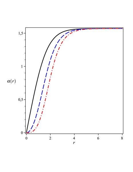
Figure 1: Numerical solutions to $\alpha(r)$ arising from (38) and (37) via (12) and (13) for $m=1$ (solid black line), $m=2$ (dashed blue line) and $m=3$ (dash-dotted red line). Here, we have chosen $h=1$, $g=2$ and $r_{0}=5$.

Moreover, for $r=0$ and $r\rightarrow\infty$, the term $\chi^{2}$ equals the unity (see the discussion after the Eq. (33)) and therefore dielectric function (35) diverges. However, such a divergence is compensated by a convenient behavior of the magnetic field $B(r)$, which avoids the first term in the right-hand side of the expression (16) for the energy density to be singular. In this case, the overall energy results in the finite value already calculated in (34).

Now, in view of the exact solution (33), the dielectric function (35) can be written in the form

$$G(r)=\frac{\left(r^{2}+r_{0}^{2}\right)^{2}}{4r^{2}r_{0}^{2}}\text{,}$$ (36)

the first-order BPS equations (28) and (29) for the $CP(2)$ sector standing for

$$\frac{d\alpha}{dr}=\pm\frac{1}{r}\left(\frac{A}{2}-m\right)\sin\alpha\text{,}$$ (37)

$$\frac{1}{r}\frac{dA}{dr}=\mp\frac{4r_{0}^{2}g^{2}h}{\left(r^{2}+r_{0}^{2}\right)^{2}}r^{2}\cos\alpha\text{.}$$ (38)

These Bogomol’nyi equations must be solved numerically by means of a finite-difference scheme according the boundary conditions (12) and (13).

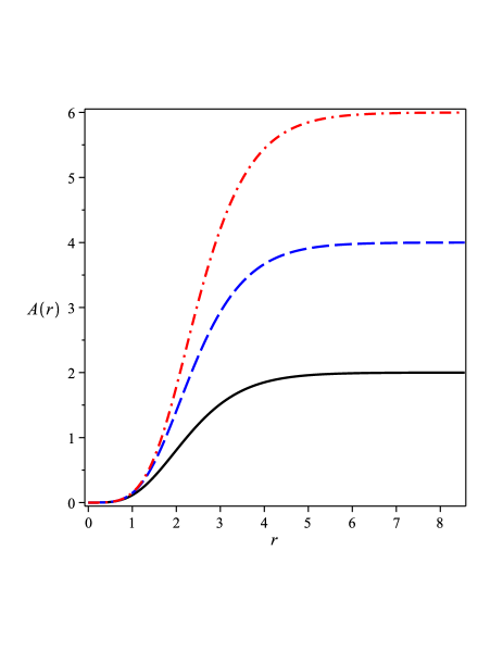
Figure 2: Numerical solutions to $A(r)$. Conventions as in the Fig. 1. The solution approaches the boundary values in a monotonic way, as expected.

We now verify the way the profiles $\alpha(r)$ and $A(r)$ approximate the boundary values. For such an analysis, we consider $m>0$ (i.e. the lower signs in the first-order equations), for the sake of simplicity. In this case, near the origin, we represent the profile fields by

$$\alpha(r)\approx\delta\alpha(r)\text{ \ \ and \ \ }A(r)\approx\delta A(r)\text{,}$$ (39)

where $\delta\alpha(r)$ and $\delta A(r)$ are small fluctuations around the boundary values. Now, substituting these representations into the first-order equations (37) and (38), and taking into account only the relevant contributions, one gets

$$\frac{d}{dr}\delta\alpha=m\frac{\delta\alpha}{r}\text{,}$$ (40)

$$\frac{d}{dr}\delta A=\frac{4g^{2}h}{r_{0}^{2}}r^{3}\text{,}$$ (41)

whose solutions provide the behavior of $\alpha(r)$ and $A(r)$, i.e.

$$\alpha(r)\approx C_{0}r^{m}\text{,}$$ (42)

$$A(r)\approx\frac{g^{2}h}{r_{0}^{2}}r^{4}\text{,}$$ (43)

where $C_{0}$ stands for a positive real constant to be determined numerically.

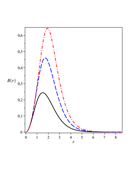
Figure 3: Numerical solutions to the modulus of the magnetic field $B(r)$. Conventions as in the Fig. 1. Here, even in the presence of topological conditions, the magnetic field mimics the nontopological behavior due to the nontrivial profile to the extra field $\chi(r)$.

A similar procedure can be implemented in order to study the behavior of the profile fields in the asymptotic limit $r\rightarrow\infty$. In this sense, we now represent these fields by

$$\alpha(r)\approx\frac{\pi}{2}-\delta\alpha(r)\text{ \ \ and \ \ }A(r)\approx 2m-\delta A(r)\text{,}$$ (44)

from which, again taking into account only the relevant contributions, one gets

$$\frac{d}{dr}\delta\alpha=-\frac{\delta A}{2r}\text{,}$$ (45)

$$\frac{d}{dr}\delta A=-4r_{0}^{2}g^{2}h\frac{\delta\alpha}{r}\text{,}$$ (46)

whose solutions allow us to conclude that the profile functions themselves behave as

$$\alpha(r)\approx\frac{\pi}{2}-C_{\infty}r^{-\sqrt{2h}r_{0}g}\text{,}$$ (47)

$$A(r)\approx 2m-2\sqrt{2h}r_{0}gC_{\infty}r^{-\sqrt{2h}r_{0}g}\text{.}$$ (48)

where $C_{\infty}$ represents an integration constant to be also determined numerically.

We now plot the numerical solutions we have found via the first-order equations (37) and (38) using the boundary conditions (12) and (13). Here, we have fixed $h=1$, $g=2$ and $r_{0}=5$, from which we have solved the equations for $m=1$ (solid black line), $m=2$ (dashed blue line) and $m=3$ (dash-dotted red line).

The figures 1 and 2 show, respectively, the numerical profiles to the $CP(2)$ scalar and gauge functions, i.e. $\alpha(r)$ and $A\left(r\right)$, from which we see that both solutions exhibit a well-defined monotonic behavior, approaching the boundary values according the approximate analytical solutions written in (42), (43), (47) and (48).

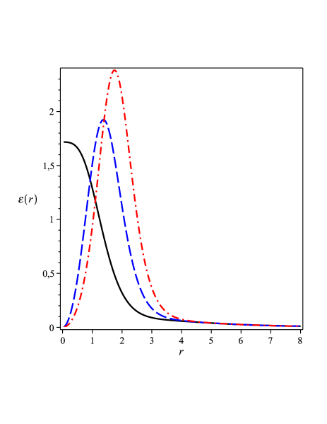
Figure 4: Numerical solutions to the energy density $\varepsilon(r)$. Conventions as in the Fig. 1. In this case, for $m=1$, one gets $\varepsilon_{bps}\left(r=0\right)=2h\left(C_{0}\right)^{2}$.

In the Figure 3, we present the numerical solutions to the modulus of the magnetic field $B(r)$. In this case, it is interesting to note how a nontrivial profile to the function $\chi(r)$ changes the shape of the corresponding magnetic sector: even in the presence of the standard topological conditions (12) and (13), the resulting magnetic field stands for a ring centered at the origin (in a dramatic contrast with its usual counterpart, which represents a lump centered at $r=0$; see the Fig. 2 of the Ref. casana ), therefore mimicking the typical nontopological behavior (see the Fig. 3 of the Ref. lima , for instance).

Moreover, given the approximate solutions (43) and (48) to the profile function $A(r)$, one gets that, near the origin, the magnetic field (9) behaves as

$$B(r)\approx-\frac{4g^{2}h}{r_{0}^{2}}r^{2}\text{,}$$ (49)

its asymptotic solution reading

$$B(r)\approx-4ghr_{0}^{2}C_{\infty}r^{-\left(\sqrt{2h}r_{0}g+2\right)}\text{,}$$ (50)

which confirm that both $B\left(r=0\right)$ and $B\left(r\rightarrow\infty\right)$ vanish, in agreement to the Figure 3.

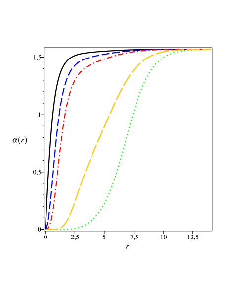
Figure 5: Numerical solutions to $\alpha(r)$ arising from (57) and (56) via (12) and (13). Conventions as in the Fig. 1. In addition, we also depict the results for $m=7$ (long-dashed orange line) and $m=10$ (dotted green line).

The Figure 4 presents the numerical profiles to the energy density $\varepsilon_{bps}(r)$. Here, it is worthwhile to point out that, for $m=1$, the energy distribution stands for a lump centered at the origin (therefore mimicking the canonical result, see the Fig. 4 of the Ref. casana ). In particular, in view of the approximate expressions (42) and (43), one gets that, near $r=0$, the energy density obeys

$$\varepsilon_{bps}(r)\approx 2h\left(C_{0}\right)^{2}+\frac{4}{r_{0}^{2}}\left(\frac{4}{r_{0}^{2}}+g^{4}h^{2}-\frac{h\left(C_{0}\right)^{4}}{6}r_{0}^{2}\right)r^{2}\text{,}$$ (51)

from which one additionally concludes that $\varepsilon_{bps}\left(r=0\right)=2h\left(C_{0}\right)^{2}$, for $m=1$.

On the other hand, for $m\neq 1$, the final configuration corresponds to a ring which, near the origin, behaves as

$$\varepsilon_{bps}(r)\approx\frac{4}{r_{0}^{2}}\left(\frac{4}{r_{0}^{2}}+g^{4}h^{2}\right)r^{2}\text{,}$$ (52)

therefore vanishing at the origin, its amplitude increasing as the vorticity $m$ itself increases. In this case, keeping the standard profile in mind, one also finds an interesting difference: in the absence of the additional terms, the energy density’s ring does not vanish at $r=0$, its amplitude decreasing as $m$ increases, see the Fig. 3 of the Ref. casana .

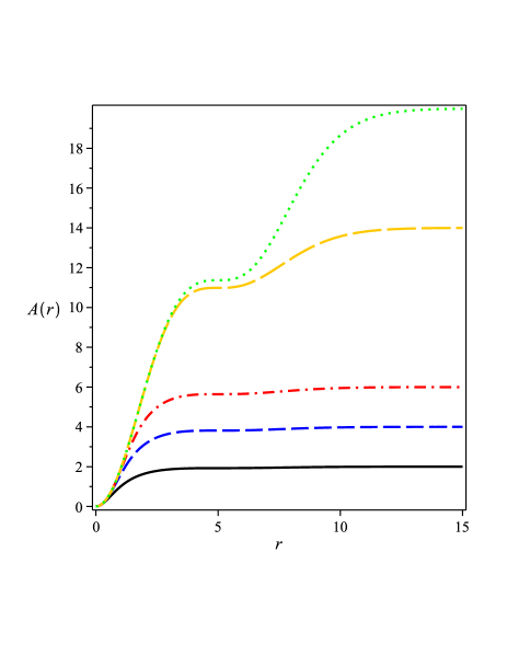
Figure 6: Numerical solutions to $A(r)$. Conventions as in the Fig. 5. In this case, as $m$ increases, $A(r)$ engenders the formation of a plateau around $r=r_{0}$.

We conclude this part by arguing that, given the solutions (47) and (48), the asymptotic one for the energy density can be verified to read

$$\varepsilon_{bps}(r)\approx\frac{16r_{0}^{4}}{r^{6}}\text{,}$$ (53)

which saturates $\varepsilon_{bps}\left(r\rightarrow\infty\right)\rightarrow 0$ (i.e. the finite energy requirement), therefore confirming the convenience of the finite energy boundary conditions (13).

III.2 The second case

We now choose the dielectric function as

$$G\left(\chi\right)=\frac{1}{\chi^{2}}\text{.}$$ (54)

In this case, given that $\chi^{2}$ calculated from (33) equals the unity at $r=0$ and $r\rightarrow\infty$, it follows from (54) that $G\left(r=0\right)=1$ and $G\left(r\rightarrow\infty\right)\rightarrow 1$. As a consequence, at the origin and asymptotically, the corresponding rotationally symmetric solitons behave as the ones arising from a simplest gauged $CP(2)$ scenario. Furthermore, at the point $r=r_{0}$, the field $\chi$ in (33) vanishes and the function $G$ in (54) diverges: in this context, such a divergence is counterbalanced by a null magnetic field at $r=r_{0}$ (therefore introducing an internal structure to the resulting vortices), from which one gets that the first term in (16) results nonsingular, the total energy then converging to the value in (34).

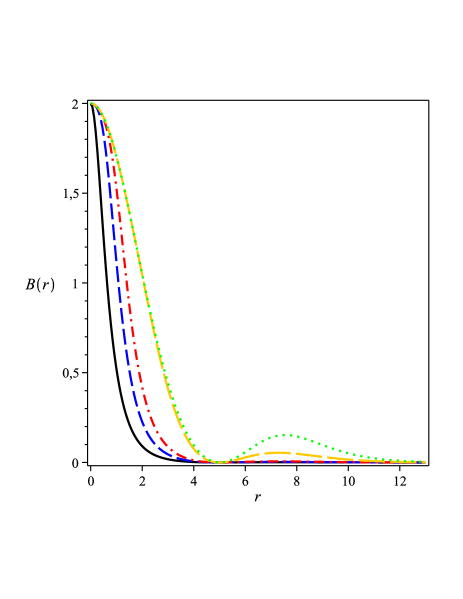
Figure 7: Numerical solutions to the modulus of the magnetic field $B(r)$. Conventions as in the Fig. 5. The magnetic sector vanishes at $r=r_{0}$, which prevents the corresponding energy distribution to be divergent.

We now use (33) in order to write (54) as

$$G(r)=\frac{\left(r^{2}+r_{0}^{2}\right)^{2}}{\left(r^{2}-r_{0}^{2}\right)^{2}}\text{,}$$ (55)

the equations (28) and (29) therefore reducing to

$$\frac{d\alpha}{dr}=\pm\frac{1}{r}\left(\frac{A}{2}-m\right)\sin\alpha\text{,}$$ (56)

$$\frac{1}{r}\frac{dA}{dr}=\mp\frac{\left(r^{2}-r_{0}^{2}\right)^{2}}{\left(r^{2}+r_{0}^{2}\right)^{2}}g^{2}h\cos\alpha\text{,}$$ (57)

These equations must be also solved numerically via the conditions (12) and (13).

We proceed to the study of the differential equations (56) and (57) near the boundaries, again for $m>0$. We begin by considering, near the origin, the profiles as represented in (39), the first-order equations satisfied by the small functions $\delta\alpha$ and $\delta A$ reading

$$\frac{d}{dr}\delta\alpha=m\frac{\delta\alpha}{r}\text{,}$$ (58)

$$\frac{d}{dr}\delta A=g^{2}hr-\frac{4g^{2}h}{r_{0}^{2}}r^{3}\text{,}$$ (59)

from which one gets the solutions

$$\alpha(r)\approx\mathcal{C}_{0}r^{m}\text{,}$$ (60)

$$A(r)\approx\frac{g^{2}h}{2}r^{2}-\frac{g^{2}h}{r_{0}^{2}}r^{4}\text{,}$$ (61)

in which the real positive constant $C_{0}$ must be determined numerically.

Likewise, in the limit $r\rightarrow\infty$, we proceed the implementation of the profile representation (44) into the BPS equations (56) and (57), from which we obtain the following linearized equations for the small functions $\delta\alpha$ and $\delta A$,

$$\frac{d}{dr}\delta\alpha=-\frac{\delta A}{2r}\text{,}$$ (62)

$$\frac{1}{r}\frac{d}{dr}\delta A=-g^{2}h\delta\alpha\text{,}$$ (63)

whose solutions allow us to write the behavior of the functions $\alpha(r)$ and $A(r)$ as

$$\alpha(r)\approx\frac{\pi}{2}-\mathcal{C}_{\infty}e^{-Mr}\text{,}$$ (64)

$$A(r)\approx 2m-g\sqrt{2h}\mathcal{C}_{\infty}re^{-Mr}\text{,}$$ (65)

where $C_{\infty}$ is an integration constant and $M$ is real parameter given by

$$M=g\sqrt{\frac{h}{2}}\text{.}$$ (66)

In this case, the exponential behavior of the asymptotic solutions (64) and (65) reveals that the real constant $M$ defined by (66) in terms of $g$ and $h$ stands for the masses of the $CP(2)$ scalar and gauge bosons inherent to the original model.

In the sequel, we depict the numerical profiles we have obtained from the first-order equations (56) and (57) via the boundary conditions (12) and (13). Here, we have chosen the same values as before for the parameters appearing in the first-order equations, i.e. $h=1$, $g=2$ and $r_{0}=5$, via which we have studied the equations for $m=1$ (solid black line), $m=2$ (dashed blue line), $m=3$ (dash-dotted red line), $m=7$ (long-dashed orange line) and $m=10$ (dotted green line).

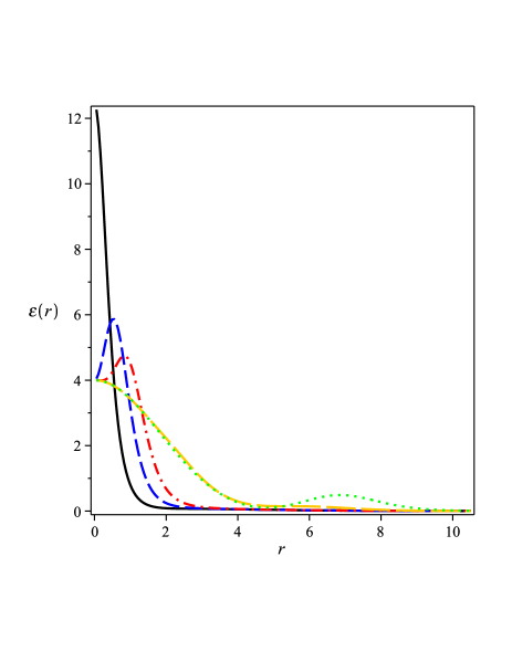
Figure 8: Numerical solutions to the energy density $\varepsilon(r)$. Conventions as in the Fig. 5. In this case, one gets $\varepsilon_{bps}\left(r=0\right)=g^{2}h^{2}+2h\left(\mathcal{C}_{0}\right)^{2}$, for $m=1$.

In the figures 5 and 6, we present the solutions to the profile functions $\alpha(r)$ and $A(r)$, respectively. Here, it is interesting to note how the shape of the solutions depend on the values of the vorticity $m$. In particular, as $m$ increases, the field $A\left(r\right)$ engenders the formation of a plateau around $r=r_{0}$ (it is instructive to compare such an effect with the one identified in the Fig. 5 of the Ref. n44 ), such an internal structure modifying the resulting magnetic field’s profile.

The Figure 7 shows the solutions to the modulus of the magnetic field $B(r)$, the corresponding configuration standing for a double-lump centered at the origin. Here, as we have argued previously, the magnetic sector vanishes at $r=r_{0}$ (such an effect being a consequence of the plateau appearing in the solution for $A(r)$), which prevents the first term in the energy distribution (16) to be divergent, the total energy therefore converging to the well-defined value in (34) (we highlight that a similar effect is shown in the Fig. 5 of the Ref. n44 ).

In addition, in view of the approximate solutions (61) and (65), it can be verified that, near $r=0$, the magnetic sector is given by

$$B(r)\approx-gh+\frac{4gh}{r_{0}^{2}}r^{2}\text{,}$$ (67)

its asymptotic counterpart standing for

$$B(r)\approx-gh\mathcal{C}_{\infty}e^{-Mr}\text{,}$$ (68)

from which one gets that $B\left(r=0\right)=-gh$ and $B\left(r\rightarrow\infty\right)\rightarrow 0$, in agreement to the Fig. 7.

We end this Section by discussing the numerical profiles to the energy density $\varepsilon_{bps}(r)$ appearing in the Figure 8. In this case, for $m=1$, the resulting configuration is a regular lump whose approximate solution, near the origin, reads

$$\varepsilon_{bps}(r)\approx g^{2}h^{2}+2h\left(\mathcal{C}_{0}\right)^{2}+\mathcal{C}_{2}r^{2}\text{,}$$ (69)

the real parameter $\mathcal{C}_{2}$ being given by

$$\mathcal{C}_{2}=2\left(\frac{8}{r_{0}^{4}}-\frac{h}{3}\left(\mathcal{C}_{0}\right)^{4}-g^{2}h^{2}\left(\frac{2}{r_{0}^{2}}+\left(\mathcal{C}_{0}\right)^{2}\right)\right)\text{,}$$ (70)

via which we conclude that $\varepsilon_{bps}\left(r=0\right)=g^{2}h^{2}+2h\left(\mathcal{C}_{0}\right)^{2}$, for $m=1$.

Moreover, for intermediate values of the vorticity, the solutions stand for well-behaved rings centered at $r=0$. However, as $m$ increases, these intermediate rings transmute to nonsingular double-lumps whose intersection occurs around $r=r_{0}$ (at this point, the energy distribution vanishes). Here, it is important to highlight that such a transmutation seems to be a new phenomenon inherent to the gauged $CP(2)$ scenario presently considered.

Finally, the reader can verify that, for $m\neq 1$, the energy distribution, near the origin, behaves as

$$\varepsilon_{bps}(r)\approx g^{2}h^{2}+\frac{4}{r_{0}^{2}}\left(\frac{4}{r_{0}^{2}}-g^{2}h^{2}\right)r^{2}\text{,}$$ (71)

which gives $\varepsilon_{bps}\left(r=0\right)=g^{2}h^{2}$. In addition, for any value of the vorticity $m$, the asymptotic solution for the energy density can be verified to be the very same one appearing in (53), therefore satisfying the finite energy requirement and the convenience of the conditions in (13).

IV Final comments

We have considered a gauged $CP(2)$ model containing an additional real scalar field which couples to the electromagnetic one via a dielectric function multiplying the usual Maxwell’s term. The stationary Gauss law tells us that the time-independent configurations have no electric charge. We have particularized our investigation by choosing well-established conventions supporting the existence of rotationally symmetric solitons with finite energy.

We then have developed the corresponding first-order framework by means of the Bogomol’nyi prescription (i.e. by minimizing the total energy of the effective model). Consequently, we have obtained the corresponding set of first-order differential equations (the Bogomol’nyi ones) engendering genuine field solutions saturating a lower-bound for the resulting energy (the Bogomol’nyi bound). It is interesting to point out that the first-order equations depend on two a priori arbitrary functions, i.e. the superpotential $\mathcal{W}(\chi)$ for the additional field $\chi$ and the dielectric function $G(\chi)$. In view of such a dependence, we have splitted our investigation into two different cases based on different choices for the dielectric function $G(\chi)$.

We have then explored such a freedom in order to construct regular first-order vortices whose shapes dramatically differ from their canonical counterparts (obtained in the absence of the additional field), the new details being understood as internal structures, as argued in the previous work n44 .

It is important to say that the results we have presented in this manuscript hold a priori only for those rotationally symmetric configurations defined by the ansatz (7) and (8), being therefore not possible to ensure that the original theory supports such a first-order framework outside the rotationally symmetric scenario, such question lying beyond the scope of this work.

Interesting ideas regarding future investigations include the search for electrically charged first-order vortices with internal structures arising from both the Chern-Simons and the Maxwell-Chern-Simons versions of the original model (1). It is also worthwhile to consider the connection between these configurations (with internal structures) and the dynamics of the gauged $CP(2)$ vortices in the presence of terms representing the effect of magnetic impurities (as studied for the Maxwell-Higgs case in the Ref. sk ), both scenarios presenting an explicit dependence of the Lagrange density on the radial coordinate $r$. These issues are presently under consideration, and we hope positive results for an incoming contribution.

- (1) N. Manton and P. Sutcliffe, Topological Solitons (Cambridge University Press, Cambridge, England, 2004).
- (2) H. B. Nielsen and P. Olesen, Nucl. Phys. B 61, 45 (1973).
- (3) M. Prasad and C. Sommerfield, Phys. Rev. Lett. 35, 760 (1975).
- (4) E. Bogomol’nyi, Sov. J. Nucl. Phys. 24, 449 (1976).
- (5) R. Jackiw and E. J. Weinberg, Phys. Rev. Lett. 64, 2234 (1990). R. Jackiw, K. Lee and E. J. Weinberg, Phys. Rev. D 42, 3488 (1990).
- (6) P. K. Ghosh, Phys. Rev. D 49, 5458 (1994).
- (7) A. M. Polyakov, Phys. Lett. B 59, 79 (1975). E. Witten, Nucl. Phys. B 149, 285 (1979). M. Shifman and A. Yung, Rev. Mod. Phys. 79, 1139 (2007).
- (8) A. Yu. Loginov, Phys. Rev. D 93, 065009 (2016).
- (9) R. Casana, M. L. Dias and E. da Hora, Phys. Lett. B 768, 254 (2017).
- (10) V. Almeida, R. Casana and E. da Hora, Phys. Rev. D 97, 016013 (2018).
- (11) R. Casana, N. H. Gonzalez-Gutierrez and E. da Hora, Topological first-order solitons in a gauged CP(2) model with the Maxwell-Chern-Simons action, arXiv:1802.10128v1 [hep-th].
- (12) E. Witten, Nucl. Phys. B 249, 557 (1985). M. Shifman, Phys. Rev. D 87, 025025 (2013).
- (13) A. Peterson, M. Shifman and G. Tallarita, Annals Phys. 353, 48 (2014); Annals Phys. 363, 515 (2015).
- (14) D. Bazeia, M. A. Marques and R. Menezes, Phys. Lett. B 780, 485 (2018).
- (15) R. A. Shelby, Science 292, 77 (2001). S. A. Ramakrishna, Rep. Prog. Phys. 68, 449 (2005). C. Caloz, Metamater. Today 12, 12 (2009).
- (16) D. Bazeia, J. Menezes and R. Menezes, Phys. Rev. Lett. 91, 241601 (2003).
- (17) R. Hobart, Proc. Phys. Soc. Lond. 82, 201 (1963). G. H. Derrick, J. Math. Phys. 5, 1252 (1964).
- (18) D. Bazeia, M. M. Doria and E. I. B. Rodrigues, Phys. Lett. A 380, 1947 (2016). D. Bazeia, J. G. G. S. Ramos and E. I. B. Rodrigues, J. Magnetism Magnetic Materials 423, 411 (2017).
- (19) D. Bazeia and A. Mohammadi, Phys. Lett. B 779, 420 (2018).
- (20) R. Casana, M. L. Dias and E. da Hora, Phys. Rev. D. 96, 076013 (2017).
- (21) A. Cockburn, S. Krusch and A. A. Muhamed, J. Math. Phys. 58, 063509 (2017).