Approximating Gaussian Process Emulators with Linear Inequality Constraints and Noisy Observations via MC and MCMC

Abstract

Adding inequality constraints (e.g. boundedness, monotonicity, convexity) into Gaussian processes (GPs) can lead to more realistic stochastic emulators. Due to the truncated Gaussianity of the posterior, its distribution has to be approximated. In this work, we consider Monte Carlo (MC) and Markov Chain Monte Carlo (MCMC) methods. However, strictly interpolating the observations may entail expensive computations due to highly restrictive sample spaces. Furthermore, having (constrained) GP emulators when data are actually noisy is also of interest for real-world implementations. Hence, we introduce a noise term for the relaxation of the interpolation conditions, and we develop the corresponding approximation of GP emulators under linear inequality constraints. We show with various toy examples that the performance of MC and MCMC samplers improves when considering noisy observations. Finally, on 2D and 5D coastal flooding applications, we show that more flexible and realistic GP implementations can be obtained by considering noise effects and by enforcing the (linear) inequality constraints.

1 Introduction

Gaussian processes (GPs) are used in a great variety of real-world problems as stochastic emulators in fields such as biology, finance and robotics (Rasmussen and Williams, 2005; Murphy, 2012). In the latter, they can be used for emulating the dynamics of robots when experiments become expensive (e.g. time consuming or highly costly) (Rasmussen and Williams, 2005).

Imposing inequality constraints (e.g. boundedness, monotonicity, convexity) into GP emulators can lead to more realistic profiles guided by the physics of data (Golchi et al., 2015; Maatouk and Bay, 2017; López-Lopera et al., 2018). Some applications where constrained GP emulators have been successfully used are computer networking (monotonicity) (Golchi et al., 2015), econometrics (positivity or monotonicity) (Cousin et al., 2016), and nuclear safety criticality assessment (positivity and monotonicity) (López-Lopera et al., 2018).

In (Maatouk and Bay, 2017; López-Lopera et al., 2018), an approximation of GP emulators based on (first-order) regression splines is introduced in order to satisfy general sets of linear inequality constraints. Because of the piecewise linearity of the finite-dimensional approximation used there, the inequalities are satisfied everywhere in the input space. Furthermore, The authors of (Maatouk and Bay, 2017; López-Lopera et al., 2018) proved that the resulting posterior distribution conditioned on both observations and inequality constraints is truncated Gaussian-distributed. Finally, it was shown in (Bay et al., 2016) that the resulting posterior mode converges uniformly to the thin plate spline solution when the number of knots of the spline goes to infinity.

Since the posterior is a truncated GP, its distribution cannot be computed in closed-form, but it can be approximated via Monte Carlo (MC) or Markov chain Monte Carlo (MCMC) (Maatouk and Bay, 2017; López-Lopera et al., 2018). Several MC and MCMC samplers have been tested in (López-Lopera et al., 2018), leading to emulators that perform well for one or two dimensional input spaces. Starting from the claim that allowing noisy observations could yield less constrained sample spaces for samplers, here we develop the corresponding approximation of constrained GP emulators when adding noise. Moreover, (constrained) GP emulators for observations that are truly noisy are also of interest for practical implementations. We test the efficiency of various MC and MCMC samplers under 1D toy examples where models without observation noise yield impractical sampling routines. We also show that, in monotonic examples, our framework can be applied up to 5D and for thousands of observations providing high-quality effective sample sizes within reasonable running times.

This paper is organised as follows. In Section 2, we introduce the finite-dimensional approximation of GP emulators with linear inequality constraints and noisy observations. In Section 3, we apply our framework to synthetic examples where the consideration of noise-free observations is unworkable. We also test it on 2D and 5D coastal flooding applications. Finally, in Section 4, we highlight the conclusions, as well as potential future works.

2 Gaussian Process Emulators with Linear Inequality Constraints and Noisy Observations

In this paper, we aim at imposing linear inequality constraints on Gaussian process (GP) emulators when observations are considered noisy. As an example, Figure 1 shows three types of GP emulators $Y$ with training points at $x_{1}=0.2$, $x_{2}=0.5$, $x_{3}=0.8$, and different inequality conditions. We used a squared exponential (SE) covariance function,

$$k_{\bm{\theta}}(x,x^{\prime})=\sigma^{2}\exp\left\{-\frac{(x-x^{\prime})^{2}}{2\ell^{2}}\right\},$$

with $\bm{\theta}=(\sigma^{2},\ell)$. We fixed the variance parameter $\sigma^{2}=0.5^{2}$ and length-scale parameter $\ell=0.2$. We set a noise variance to be equal to 0.5% of the variance parameter $\sigma^{2}$. One can observe that different types of (constrained) Gaussian priors (top) yield different GP emulators (bottom) for the same training data. One can also note that the interpolation constraints are relaxed due to the noise effect, and that the inequality constraints are still satisfied everywhere.

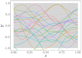
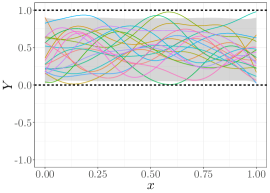
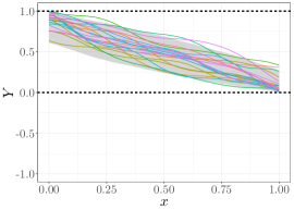
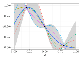
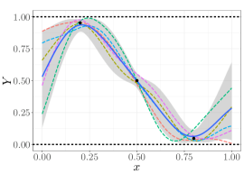
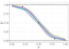
Figure 1: GP emulators under no constraints (left), boundedness constraints $Y\in[0,1]$ (centre), boundedness $Y\in[0,1]$ and non-increasing constraints (right). Samples from the different types of (constrained) Gaussian priors and the resulting GP emulators are shown in the first and second row, respectively. Each panel shows: the conditional emulations (dashed lines), and the 95% prediction interval (grey region). For boundedness constraints, bounds at $l=0$ and $u=1$ correspond to horizontal dashed lines. For GP emulators, the conditional mean (blue solid line) and interpolation points (dots) are also shown.

Next, we formally introduce the corresponding model to obtain constrained GP emulators with linear inequality constraints and noisy observations as in Figure 1.

2.1 Finite-Dimensional Approximation of Gaussian Process Emulators with Noisy Observations

Let $Y$ be a centred GP on $\mathbb{R}$ with arbitrary covariance function $k$. Consider $x\in\mathcal{D}$, with space $\mathcal{D}=[0,1]$. For simplicity, consider a spline decomposition with an equispaced set of knots $t_{1},\cdots,t_{m}\in\mathcal{D}$ such that $t_{j}=(j-1)\Delta_{m}$ for $j=1,\cdots,m$, with $\Delta_{m}=1/(m-1)$. This assumption can be relaxed for non-equispaced designs of knots as in (Larson and Bengzon, 2013), leading to similar developments as obtained in this paper but with slight differences when imposing the inequality constraints (e.g. convexity condition). In contrast to (López-Lopera et al., 2018), here we consider noisy observations $y_{i}\in\mathbb{R}$ for $i=1,\cdots,n$. Define $Y_{m}$ as a stochastic emulator consisting of the piecewise-linear interpolation of $Y$ at knots $(t_{1},\cdots,t_{m})$,

$$Y_{m}(x)=\sum_{j=1}^{m}\phi_{j}(x)Y(t_{j}),\quad\mbox{s.t.}\quad Y_{m}(x_{i})+\varepsilon_{i}=y_{i}\ \mbox{(interpolation constraints)},$$ (1)

where $x_{i}\in\mathcal{D}$, $\varepsilon_{i}\sim\mathcal{N}\left({0,\tau^{2}}\right)$ for $i=1,\cdots,n$, with noise variance $\tau^{2}$, and $\phi_{1},\cdots,\phi_{m}$ are hat basis functions given by

$$\phi_{j}(x):=\begin{cases}1-\left|\frac{x-t_{j}}{\Delta_{m}}\right|&\mbox{if }\left|\frac{x-t_{j}}{\Delta_{m}}\right|\leq 1,\\ 0&\mbox{otherwise}.\end{cases}$$ (2)

As in many classical GP implementations (Rasmussen and Williams, 2005), we assume that $\varepsilon_{1},\cdots,\varepsilon_{n}$ are independent, and independent of $Y$. However, since the framework proposed here does not have any restriction on the type of the covariance function, the extension to other noise distributions and/or noise with autocorrelation can be done as in standard GP implementations (Rasmussen and Williams, 2005; Murphy, 2012).

One must note that the benefit of considering noisy observations in (1) is that, due to the “relaxation” of the interpolation conditions, the number of knots $m$ does not have to be larger than the number of interpolation points $n$ (assumption required in (López-Lopera et al., 2018) for the interpolation of noise-free observations). Then, for $m\ll n$, the finite representation in (1) would lead to less expensive procedures since the cost of the MC and MCMC procedures below grow with the value of $m$ rather than $n$ (see Sections 2.2 and 2.3).

2.2 Imposing Linear Inequality Constraints

Now, assume that $Y_{m}$ also satisfies inequality constraints everywhere in the input space (e.g. boundedness, monotonicity, convexity), i.e.

$$Y_{m}\in\mathcal{E}\quad\mbox{(inequality constraints)},$$ (3)

where $\mathcal{E}$ is a convex set of functions defined by some inequality conditions. Then, the benefit of using (1) is that, for many constraint sets $\mathcal{E}$, satisfying $Y_{m}\in\mathcal{E}$ is equivalent to satisfying only a finite number of inequality constraints at the knots $(Y(t_{1}),\cdots,Y(t_{m}))$ (Maatouk and Bay, 2017), i.e.

$$Y_{m}\in\mathcal{E}\;\;\Leftrightarrow\;\;\bm{\xi}\in\mathcal{C},$$ (4)

with $\xi_{j}:=Y(t_{j})$ for $j=1,\cdots,m$, and $\mathcal{C}$ a convex set on $\mathbb{R}^{m}$. As an example, when we evaluate a GP with bounded trajectories $l\leq Y_{m}(x)\leq u$, the convex set $\mathcal{C}$ can be defined by $\mathcal{C}_{[l,u]}:=\{\textbf{c}\in\mathbb{R}^{m};\ \forall\ j=1,\cdots,m\ :l\leq\ c_{j}\leq u\}$. In this paper, we consider the case where $\mathcal{C}$ is composed by a set of $q$ linear inequalities of the form

$$\mathcal{C}=\bigg{\{}\textbf{c}\in\mathbb{R}^{m};\ \forall\;k=1,\dots,q\;:\;l_{k}\leq\sum_{j=1}^{m}\lambda_{k,j}c_{j}\leq u_{k}\bigg{\}},$$ (5)

where the $\lambda_{k,j}$’s encode the linear operations, the $l_{k}$’s and $u_{k}$’s represent the lower and upper bounds, respectively. One can note that the convex set $\mathcal{C}_{[l,u]}$ is a particular case of $\mathcal{C}$ where $\lambda_{k,j}=1$ if $k=j$ and zero otherwise, and with bounds $l_{k}=l$, $u_{k}=u$, for $k=1,\cdots,m$.

We now aim at computing the distribution of $Y_{m}$ conditionally on the constraints in (1) and (3). One can observe that the vector $\bm{\xi}$ is a centred Gaussian vector with covariance matrix $\bm{\Gamma}=(k(t_{i},t_{j}))_{1\leq i,j\leq m}$. Denote $\bm{\Lambda}=(\lambda_{k,j})_{1\leq k\leq q,1\leq j\leq m}$, $\bm{l}=(\ell_{k})_{1\leq k\leq q}$, $\bm{u}=(u_{k})_{1\leq k\leq q}$, $\bm{\Phi}$ the $n\times m$ matrix defined by $\bm{\Phi}_{i,j}=\phi_{j}(x_{i})$, and $\bm{y}=[y_{1},\cdots,y_{n}]^{\top}$ the vector of noisy observations at points $x_{1},\cdots,x_{n}$. Then, the distribution of $\bm{\xi}$ conditioned on $\bm{\Phi}\bm{\xi}+\bm{\varepsilon}=\bm{y}$, with $\bm{\varepsilon}\sim\mathcal{N}\left({\bm{0},\tau^{2}\bm{I}}\right)$, is given by (Rasmussen and Williams, 2005)

$$\bm{\xi}|\{\bm{\Phi}\bm{\xi}+\bm{\varepsilon}=\bm{y}\}\sim\mathcal{N}(\bm{\mu},\bm{\Sigma}),$$ (6)

where

$$\bm{\mu}=\bm{\Gamma}\bm{\Phi}^{\top}[\bm{\Phi}\bm{\Gamma}\bm{\Phi}^{\top}+\tau^{2}\bm{I}]^{-1}\bm{y},\quad\mbox{and}\quad\bm{\Sigma}=\bm{\Gamma}-\bm{\Gamma}\bm{\Phi}^{\top}[\bm{\Phi}\bm{\Gamma}\bm{\Phi}^{\top}+\tau^{2}\bm{I}]^{-1}\bm{\Phi}\bm{\Gamma}.$$ (7)

One can note that, in the limit as the noise variance $\tau^{2}\to\infty$, then $\bm{\mu}\to\bm{0}$ and $\bm{\Sigma}\to\bm{\Gamma}$, and therefore the distribution in (6) ignores the observations $\bm{y}$. In that case, MC and MCMC samplers are performed in the sample space of the prior of $\bm{\xi}$, which is less restrictive than the one of $\bm{\xi}|\{\bm{\Phi}\bm{\xi}+\bm{\varepsilon}=\bm{y}\}$. Since the inequality constraints are on $\bm{\Lambda}\bm{\xi}$, one can first show that the posterior distribution of $\bm{\Lambda}\bm{\xi}$ conditioned on $\bm{\Phi}\bm{\xi}+\bm{\varepsilon}=\bm{y}$ and $\bm{l}\leq\bm{\Lambda}\bm{\xi}\leq\bm{u}$ is truncated Gaussian-distributed (see, e.g., López-Lopera et al., 2018, for further discussion when noise-free observations are considered), i.e.

$$\bm{\Lambda}\bm{\xi}|\{\bm{\Phi}\bm{\xi}+\bm{\varepsilon}=\bm{y},\bm{l}\leq\bm{\Lambda}\bm{\xi}\leq\bm{u}\}\sim\mathcal{TN}\left({\bm{\Lambda}\bm{\mu},\;\bm{\Lambda}\bm{\Sigma}\bm{\Lambda}^{\top},\;\bm{l},\;\bm{u}}\right).$$ (8)

Notice that the inequality constraints are encoded in the posterior mean $\bm{\Lambda}\bm{\mu}$, the posterior covariance $\bm{\Lambda}\bm{\Sigma}\bm{\Lambda}^{\top}$, and the bounds $(\bm{l},\bm{u})$. Moreover, one must also highlight that by considering noisy observations, due to the “relaxation” of the interpolation conditions, inequality constraints can be imposed also when the observations $(y_{1},\cdots,y_{n})$ do not fulfil the inequalities.

Finally, the truncated Gaussian distribution in (8) does not have a closed-form expression but it can be approximated via MC or MCMC. Hence, samples of $\bm{\xi}$ can be recovered from samples of $\bm{\Lambda}\bm{\xi}$, by solving a linear system (López-Lopera et al., 2018). As discussed in (López-Lopera et al., 2018), the number of inequalities $q$ is usually larger than the number of knots $m$ for many convex sets $\mathcal{C}$. If we further assume that $q\geq m$, and that $\operatorname{rank}(\bm{\Lambda})=m$, then the solution of the linear system $\bm{\Lambda}\bm{\xi}$ exists and is unique (see López-Lopera et al., 2018, for a further discussion). Therefore, samples of $Y_{m}$ can be obtained from samples of $\bm{\xi}$, with the formula $Y_{m}(x)=\sum_{j=1}^{m}\phi_{j}(x)\xi_{j}$ for $x\in\mathcal{D}$. The implementation of the GP emulator $Y_{m}$ is summarised in Algorithm 1.

Algorithm 1 GP emulator with linear inequality constraints.

1:REQUIRE: $\bm{y}\in\mathbb{R}^{n}$, $\bm{\Gamma}\in\mathbb{R}^{m\times m}$, $\tau^{2}\in\mathbb{R}^{+}$, $\bm{\Phi}\in\mathbb{R}^{n\times m}$, $\bm{\Lambda}\in\mathbb{R}^{q\times m}$, $\bm{l}\in\mathbb{R}^{q}$, $\bm{u}\in\mathbb{R}^{q}$

2:ENSURE: Emulated samples from $\bm{\xi}|\{\bm{\Phi}\bm{\xi}+\bm{\varepsilon}=\bm{y},\bm{l}\leq\bm{\Lambda}\bm{\xi}\leq\bm{u}\}$

3:Compute the conditional mean and covariance of $\bm{\xi}|\{\bm{\Phi}\bm{\xi}+\bm{\varepsilon}=\bm{y}\}$,

4:    $\bm{\mu}=\bm{\Gamma}\bm{\Phi}^{\top}(\bm{\Phi}\bm{\Gamma}\bm{\Phi}^{\top}+\tau^{2}\bm{I})^{-1}\bm{y}$,

5:    $\bm{\Sigma}=\bm{\Gamma}-\bm{\Gamma}\bm{\Phi}^{\top}(\bm{\Phi}\bm{\Gamma}\bm{\Phi}^{\top}+\tau^{2}\bm{I})^{-1}\bm{\Phi}\bm{\Gamma}$.

6:Sample $\bm{z}$ from the truncated Gaussian distribution via MC/MCMC,

7:    $\bm{z}=\bm{\Lambda}\bm{\xi}|\{\bm{\Phi}\bm{\xi}+\bm{\varepsilon}=\bm{y},\textbf{{l}}\leq\bm{\Lambda}\bm{\xi}\leq\textbf{{u}}\}\sim\mathcal{TN}\left({\bm{\Lambda}\bm{\mu},\;\bm{\Lambda}\bm{\Sigma}\bm{\Lambda}^{\top},\;\bm{l},\;\bm{u}}\right).$

8:Compute $\bm{\xi}$ by solving the linear system $\bm{\Lambda}\bm{\xi}=\bm{z}$.

2.3 Maximum a Posteriori Estimate via Quadratic Programming

In practice, the posterior mode (maximum a posteriori estimate, MAP) of (8) can be used as a point estimate of unobserved quantities (Rasmussen and Williams, 2005), and as a starting state of MCMC samplers (Murphy, 2012). Let $\bm{\mu}^{\ast}$ be the posterior mode that maximises the probability density function (pdf) of $\bm{\xi}$ conditioned on $\bm{\Phi}\bm{\xi}+\bm{\varepsilon}=\bm{y}$ and $\bm{l}\leq\bm{\Lambda}\bm{\xi}\leq\bm{u}$. Then, maximising the pdf in (8) is equivalent to maximise the quadratic problem

$$\bm{\mu}^{\ast}=\underset{\bm{\xi}\text{ s.t. }\bm{l}\leq\bm{\Lambda}\bm{\xi}\leq\bm{u}}{\arg\max}\{-[\bm{\xi}-\bm{\mu}]^{\top}\bm{\Sigma}^{-1}[\bm{\xi}-\bm{\mu}]\},$$ (9)

with conditional mean $\bm{\mu}$ and conditional covariance $\bm{\Sigma}$ as in (7). By maximising (9), we are looking for the most likely vector $\bm{\xi}$ satisfying both the interpolation and inequality constraints (Bishop, 2007). One must highlight that the posterior mode of (8) converges uniformly to the spline solution when the number of knots $m\to\infty$ (Maatouk and Bay, 2017; Bay et al., 2016). Finally, the optimisation problem in (9) is equivalent to

$$\bm{\mu}^{\ast}=\underset{\bm{\xi}\text{ s.t. }\bm{l}\leq\bm{\Lambda}\bm{\xi}\leq\bm{u}}{\arg\min}\{\bm{\xi}^{\top}\bm{\Sigma}^{-1}\bm{\xi}-2\bm{\mu}^{\top}\bm{\Sigma}^{-1}\bm{\xi}\},$$ (10)

which can be solved via quadratic programming (Goldfarb and Idnani, 1982).

2.4 Extension to Higher Dimensions

The GP emulator of Section 2 can be extended to $d$ dimensional input spaces by tensorisation (see, e.g., Maatouk and Bay, 2017; López-Lopera et al., 2018, for a further discussion on imposing inequality constraints for $d\geq 2$). Consider $\bm{x}=(x_{1},\cdots,x_{d})\in\mathcal{D}$ with input space $\mathcal{D}=[0,1]^{d}$, and a set of knots per dimension $(t_{1}^{1},\cdots,t_{m_{1}}^{1}),\cdots,(t_{1}^{d},\cdots,t_{m_{d}}^{d})$. Then, the GP emulator $Y_{m_{1},\cdots,m_{d}}$ is given by

$$Y_{m_{1},\cdots,m_{d}}(\bm{x})=\sum_{j_{1}=1,\cdots,m_{1}}\cdots\sum_{j_{d}=1,\cdots,m_{d}}[\phi_{j_{1}}^{1}(x_{1})\times\cdots\times\phi_{j_{d}}^{d}(x_{d})]\xi_{j_{1},\cdots,j_{d}},$$ (11)

with $\bm{x}_{i}\in\mathcal{D}$ for $i=1,\cdots,n$, $\xi_{j_{1},\cdots,j_{d}}:=Y(t_{j_{1}},\cdots,t_{j_{d}})$, and $\phi_{j_{\kappa}}^{\kappa}$ are hat basis functions as defined in (2). We aim at computing (11) subject to some interpolation constraints $Y_{m_{1},\cdots,m_{d}}\left(\bm{x}_{i}\right)+\varepsilon_{i}=y_{i}$, with $y_{i}\in\mathbb{R}$ and $\varepsilon_{i}\sim\mathcal{N}\left({0,\tau^{2}}\right)$ for $i=1,\cdots,n$; and inequality constraints $\bm{\xi}=[\xi_{1,\cdots,1},\cdots,\xi_{m_{1},\cdots,m_{d}}]^{\top}\in\mathcal{C}$ with $\mathcal{C}$ a convex set of $\mathbb{R}^{m_{1}\times\cdots\times m_{d}}$. We assume that $\varepsilon_{1},\cdots,\varepsilon_{n}$ are independent, independent of $Y$. Then, following a similar procedure as in Section 2, Algorithm 1 can be used with $\bm{\xi}$ a centred Gaussian vector with an arbitrary covariance matrix $\bm{\Gamma}$.

Notice that having less knots than observations can have a great impact since the MC and MCMC samplers will then be performed in low dimensional spaces when $m=m_{1}\times\cdots\times m_{d}\ll n$. For the case $m\ll n$, the inversion of the matrix $(\bm{\Phi}\bm{\Gamma}\bm{\Phi}^{\top}+\tau^{2}\bm{I})\in\mathbb{R}^{n\times n}$ can be computed more efficiently through the matrix inversion lemma (Press et al., 1992), reducing the computational complexity to the inversion of an $m\times m$ full-rank matrix. Therefore, the computation of the conditional distribution in (7) and the estimation of the covariance parameter can be achieved faster. Moreover, due to the relaxation of the interpolation conditions through a noise effect, MC and MCMC samplers are performed in less restrictive sample spaces, and this leads to faster emulators.

3 Numerical Experiments

The codes were implemented in the R programming language, based on the open source package lineqGPR (López-Lopera, 2018). This package is based on previous R software developments produced by the Dice (Deep Inside Computer Experiments) and ReDice Consortiums (e.g. DiceKriging, Roustant et al. (2012); DiceDesign, Dupuy et al. (2015); kergp Deville et al. (2015)), but incorporating some structures of classic libraries for GP regression modelling from other platforms (e.g. the GPmat toolbox from MATLAB, and the GPy library from Python).

lineqGPR also contains implementations of different samplers for the approximation of truncated (multivariate) Gaussian distribution. Samplers are based on recent contributions on efficient MC and MCMC inference methods. Table 1 summarise some properties of the different MC and MCMC samplers used in this paper (see, e.g., Maatouk and Bay, 2016; Botev, 2017; Taylor and Benjamini, 2017; Pakman and Paninski, 2014, for a further discussion).

Table 1: Comparison between the different MC and MCMC samplers provided in lineqGPR: rejection sampling from the mode (RSM) (Maatouk and Bay, 2016), exponential tilting (ExpT) (Botev, 2017), Gibbs sampling (Taylor and Benjamini, 2017), and exact Hamiltonian monte carlo (HMC)(Pakman and Paninski, 2014).

Item	RSM	ExpT	Gibbs	HMC
Exact method	✓	✓	✗	✗
Non parametric	✓	✓	✓	✓
Acceptance rate	low	high	100%	100%
Speed	slow	fast	slow-fast	fast
Uncorrelated samples	✓	✓	✗	✗
Previous R Implementations	constrKriging	TruncatedNormal	tmvtnorm	tmg

Codes were executed on a single core of an Intel^® Core^TM i7-6700HQ CPU.

3.1 1D Toy Example under Boundedness Constraint

Here, we use the GP framework introduced in Section 2 for emulating bounded trajectories $Y_{m}\in[-\alpha,\alpha]$ with constant $\alpha\in\mathbb{R}$. We aim at analysing the resulting constrained GP emulator when noise-free or noisy observations are considered. The dataset is $(x_{i},y_{i})_{1\leq i\leq 5}$: $(0,0)$, $(0.2,-0.5)$, $(0.5,-0.3)$, $(0.75,0.5)$, and $(1,0.4)$. We use a Matérn 5/2 covariance function,

$$k_{\bm{\theta}}(x,x^{\prime})=\sigma^{2}\left(1+\frac{\sqrt{5}|x-x^{\prime}|}{\ell}+\frac{5}{3}\frac{(x-x^{\prime})^{2}}{\ell^{2}}\right)\exp\left\{-\frac{\sqrt{5}|x-x^{\prime}|}{\ell}\right\},$$

with $\bm{\theta}=(\sigma^{2},\ell)$. We fix the variance parameter $\sigma^{2}=10$ leading to highly variable trajectories. The lengthscale parameter $\ell$ and the noise variance $\tau^{2}$ are estimated via maximum likelihood (ML).

The effect of different bounds $[-\alpha,\alpha]$ on the constrained GP emulators can be seen in Figure 2. There, we set $m=100$ for having emulations with high-quality of resolution, and we generated $10^{4}$ constrained emulations via RSM (Maatouk and Bay, 2016). One can observe that, since interpolation conditions were relaxed due to the influence of the noise variance $\tau^{2}$, the prediction intervals are wider when bounds become closer to the observations. For the case $\alpha=0.5$, the noise-free GP emulator yielded costly procedures due to a small acceptance rate equal to $0.1\%$. In contrast, when noisy observations were assumed, emulations were more likely to be accepted leading to an acceptance rate equal to $16.92\%$.

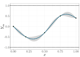
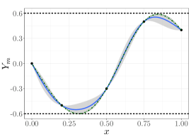
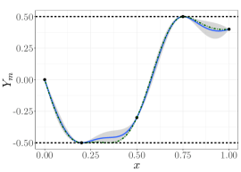
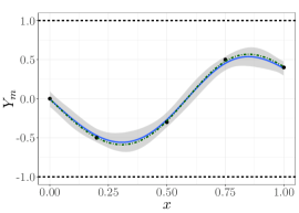
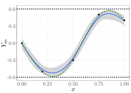
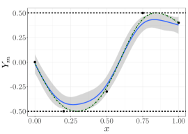
Figure 2: GP emulators under boundedness constraints $Y_{m}\in[-\alpha,\alpha]$. Results are shown considering (top) noise-free and (bottom) noisy observations: (left) $\alpha=1$, (centre) $\alpha=0.6$, and (right) $\alpha=0.5$. Each panel shows: the observations (dots), the conditional mean (solid line), the conditional mode (dot-dash line), the 95% prediction interval (grey region), and the bounds (dashed lines).

Now, we assess all the MC and MCMC methods from Table 1 for the approximation of the truncated Gaussian posterior distribution in (8). We considered the examples from Figure 2. For the MCMC samplers, we used the posterior mode solution from (10) as the starting state of the Markov chains. This initialises the chains in a high probability region. Therefore, only few emulations have been “burned” in order to have samples that appeared to be independent of the starting state. Here, we only burned the first 100 emulations. We evaluated the performance of both MC and MCMC samplers in terms of the effective sample size (ESS):

$$\operatorname{ESS}=\frac{n_{s}}{1+2\sum_{k=1}^{n_{s}}\rho_{k}},$$ (12)

where $n_{s}$ is the size of the sample path, and $\rho_{k}$ is the sample autocorrelation with lag $k$. The ESS indicator gives an intuition on how many emulations of the sample path can be considered independent (Gong and Flegal, 2016). In order to obtain non-negative sample autocorrelations $\rho_{k}$, we used the convex sequence estimator proposed in (Geyer, 1992). We then computed the ESS of each coordinate of $\bm{\xi}\in\mathbb{R}^{m}$, i.e. $\operatorname{ESS}_{j}=\operatorname{ESS}(\xi_{j}^{1},\cdots,\xi_{j}^{n_{s}})$ for $j=1,\cdots,m$, and we evaluated the quantiles $(q_{10\%},q_{50\%},q_{90\%})$ over the $m$ resulting $\operatorname{ESS}$ values. The sample size $n_{s}=10^{4}$ has been chosen to be larger than the minimum ESS required to obtain a proper estimation of the vector $\bm{\xi}\in\mathbb{R}^{m}$ (Gong and Flegal, 2016). Finally, we tested the efficiency of each sampler by computing the time normalised ESS (TN-ESS) (Lan and Shahbaba, 2016) at $q_{10\%}$ (worst case): $\operatorname{TN-ESS}=q_{10\%}(\operatorname{ESS})/\operatorname{(CPU\ Time)}$.

Table 2 displays the performance indicators obtained for each samplers from Table 1. Firstly, one can observe that RSM yielded the most expensive procedures due to its high rejection rate when sampling the constrained trajectories from the posterior mode. In particular, for $\alpha=0.5$, and assuming noise-free observations, the prohibitively small acceptance rate of RSM led to costly procedures (about 7 hours) making it impractical. Secondly, although the Gibbs sampler needs to discard intermediate samples (thinning effect), it provided accurate ESS values within a moderate running time (with effective sampling rates of $400\ s^{-1}$). Thirdly, due to the high acceptance rates obtained by ExpT, and good exploratory behaviour of the exact HMC, both samplers provided much more efficient TN-ESS values compared to their competitors, generating thousands of effective emulations each second. Finally, as we expected, the performance of some samplers were improved when adding a noise. For RSM, due to the relaxation of the interpolation conditions, we noted that emulations were more likely to be accepted leading quicker routines: more than 150 times faster with noise (see Table 2, $\alpha=0.5$).

Table 2: Efficiency of MC and MCMC from Table 1 for emulating bounded samples $Y_{m}\in[-\alpha,\alpha]$ of Figure 2. Best results are shown in bold. For the Gibbs sampler, we set the thinning parameter to 200 emulations aiming to obtain competitive ESS values with respect to other samplers. ^†Results could not be obtained due to numerical instabilities.

Bounds	Method	Without noise variance			With noise variance
		CPU Time	ESS $[\times 10^{4}]$	TN-ESS	CPU Time	ESS $[\times 10^{4}]$	TN-ESS
		$[s]$	$(q_{10\%},q_{50\%},q_{90\%})$	$[\times 10^{4}s^{-1}]$	$[s]$	$(q_{10\%},q_{50\%},q_{90\%})$	$[\times 10^{4}s^{-1}]$
[-1.0, 1.0]	RSM	61.30	(0.97, 1.00, 1.00)	0.02	57.64	(0.91, 1.00, 1.00)	0.02
	ExpT	2.30	(0.98, 1.00, 1.00)	0.43	2.83	(0.96, 1.00, 1.00)	0.34
	Gibbs	19.70	(0.84, 0.86, 0.91)	0.04	21.18	(0.75, 0.84, 0.91)	0.04
	HMC	1.89	(0.95, 0.99, 1.00)	0.50	1.92	(0.94, 0.99, 1.00)	0.49
[-0.75, 0.75]	RSM	63.59	(1.00, 1.00, 1.00)	0.02	48.66	(0.95, 0.99, 1.00)	0.02
	ExpT	3.22	(0.96, 0.99, 1.00)	0.30	3.24	(0.98, 1.00, 1.00)	0.30
	Gibbs	20.20	(0.83, 0.86, 0.91)	0.04	18.23	(0.74, 0.84, 0.93)	0.04
	HMC	1.46	(0.94, 1.00, 1.00)	0.64	1.28	(0.94, 0.97, 1.00)	0.73
[-0.6, 0.6]	RSM	242.34	(0.94, 0.97, 1.00)	0	101.20	(0.96, 1.00, 1.00)	0.01
	ExpT	2.94	(0.94, 1.00, 1.00)	0.32	2.80	(0.98, 1.00, 1.00)	0.35
	Gibbs	18.89	(0.80, 0.83, 0.94)	0.04	18.90	(0.77, 0.84, 0.92)	0.04
	HMC	1.72	(0.92, 0.99, 1.00)	0.53	1.68	(0.93, 0.96, 1.00)	0.55
[-0.5, 0.5]	RSM	25512.77	(0.98, 1.00, 1.00)	0	157.06	(0.96, 0.99, 1.00)	0.01
	ExpT	2.50	(0.99, 1.00, 1.00)	0.40	2.69	(0.97, 1.00, 1.00)	0.36
	Gibbs†	—	—	—	—	—	—
	HMC	6.20	(0.86, 0.90, 0.98)	0.14	2.14	(0.52, 0.85, 0.97)	0.24

Finally, we assess the efficiency of the HMC sampler in terms of its mixing performance (see Figure 3). We analyse the example of Figure 2 using the noisy GP emulator with $\alpha=0.5$. From both the trace and autocorrelation plots at $Y_{m}(0.01)$, one can conclude that the HMC sampler mixes well with small correlations.

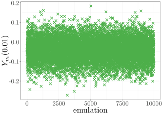
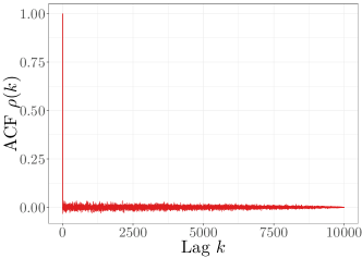
Figure 3: Efficiency of the HMC sampler in terms of its mixing performance. Results are shown for the (left) trace and (right) autocorrelation plots at $Y_{m}(0.01)$.

3.2 1D Toy Example under Multiple Constraints

In (López-Lopera et al., 2018), numerical implementations were limited to noise-free observations that fulfilled the inequality constraints. In this example, we test the case when noisy observations do not necessarily satisfy the inequalities.

Consider the sigmoid function given by

$$x\mapsto\frac{1}{1+\exp\big{\{}-10(x-\frac{1}{2})\big{\}}},\ \mbox{ for }\ x\in[0,1].$$ (13)

We evaluated (13) at $n=300$ random values of $x$, and we contaminated the function evaluations with an additive Gaussian white noise with a standard deviation equal to 10% of the sigmoid range. Since (13) exhibits both boundedness and non-decreasing conditions, we added those constraints into the GP emulator $Y_{m}$ using the convex set

$$\mathcal{C}_{[0,1]}^{\uparrow}=\bigg{\{}\textbf{c}\in\mathbb{R}^{m};\ \forall j=2,\cdots,m\ :\ c_{j}\geq c_{j-1},\ c_{1}\geq 0,\ c_{m}\leq 1\bigg{\}}.$$

Hence, the MC and MCMC samplers will be performed on $\mathbb{R}^{m+1}$ (number of inequality conditions). As a covariance function, we used a SE kernel, and we estimated the parameters $(\sigma^{2},\ell,\tau^{2})$ via ML.

Unlike (López-Lopera et al., 2018), there is no need here to satisfy the condition $m\geq n$, due to the noise. Therefore, the finite approximation of Section 2 can be seen as a surrogate model of standard GP emulators for $m\ll n$. Figure 4 shows the performance of the constrained emulators via HMC for $m=5,25,100$. For smaller values of $m$, the GP emulator runs fast but with a low quality of resolution of the approximation. For example, for $m=5$, because of the linearity assumption between knots, the predictive mean presents breakpoints at the knots. On the other hand, the GP emulator yields smoother (constrained) emulations as $m$ increases ($m\geq 25$). In particular, one can observe that for $m=25$, the emulator leads to a good trade-off between quality of resolution and running time (13 times faster than for $m=100$).

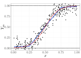
(a) $m=5$, $\text{CPU Time}=0.03\ s$

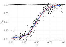
(b) $m=25$, $\text{CPU Time}=0.09\ s$

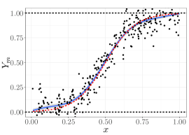
(c) $m=100$, $\text{CPU Time}=1.20\ s$

Figure 4: GP emulators under boundedness and monotonicity constraints. Results are shown for different number values of knots $m$. Each panel shows: the target function (dashed lines), the noisy training points (dots), the conditional mean (solid line), the 95% prediction interval (grey region), and the bounds (horizontal dashed lines).

Finally, we test the performance of the proposed framework under different regularity assumptions, noise levels and inequality constraints. For the example in Figure 4, we fixed $m=200$ and used different choices of covariance functions: either a Matérn 3/2 kernel, a Matérn 5/2 kernel or a SE kernel. Given a fixed noise level, the covariance parameters of each GP model, i.e. $\bm{\theta}=(\sigma^{2},\ell)$, were estimated via ML. The noise levels were chosen using different proportions of the sigmoid range. We assessed the proposed GP emulator accounting for either boundedness constraints, monotonicity constraints or both. We computed the CPU time and the $Q^{2}$ criterion. The $Q^{2}$ criterion is given by $Q^{2}=1-\operatorname{SMSE}$, where SMSE is the standardised mean squared error (Rasmussen and Williams, 2005), and is equal to one if the predictive mean is equal to the test data and lower than one otherwise. We used the 300 noise-free function evaluations from (13) as test data. Results are shown in Table 3. One can note that the introduction of noise let us also have constrained GP emulations in the cases where the regularity of the GP prior is not in agreement with the regularity of data and the inequality conditions. In particular, expensive procedures were obtained for the Matérn 3/2 kernel when considering monotonicity. In those cases, the high irregularity of the (unconstrained) GP prior yielded more restrictive sample spaces that fulfil the monotonicity conditions. Furthermore, one may observe that the computational cost of emulators can be attenuated by increasing the noise level but at the cost of the accuracy of predictions.

Table 3: Performance of the GP emulators from Figure 4 under different regularity assumptions, noise levels and inequality constraints. The noise levels were chosen using different proportions of the range of the sigmoid function in (13). CPU Time $[s]$ and $Q^{2}$ $[\%]$ results are shown for various covariance function (i.e. Matérn 3/2 kernel, Matérn 5/2 kernel and SE kernel), and different inequality constraints.

Noise	Boundedness Constraints
level	Matérn$\frac{3}{2}$		Matérn$\frac{5}{2}$		SE
	Time	$Q^{2}$	Time	$Q^{2}$	Time	$Q^{2}$
0%	—	—	—	—	—	—
0.5%	1.0	99.4	0.8	99.6	0.6	99.7
1.0%	1.1	99.4	0.7	99.6	0.6	99.7
5.0%	1.0	98.9	0.8	99.3	0.6	99.5
10.0%	0.9	98.2	0.8	98.9	0.6	99.2

Noise	Monotonicity Constraints
level	Matérn$\frac{3}{2}$		Matérn$\frac{5}{2}$		SE
	Time	$Q^{2}$	Time	$Q^{2}$	Time	$Q^{2}$
0%	—	—	—	—	—	—
0.5%	117.0	99.5	1.4	99.8	1.2	99.8
1.0%	14.5	99.1	1.2	99.8	1.0	99.8
5.0%	7.4	95.6	1.0	99.3	0.8	99.3
10.0%	6.3	91.9	1.0	98.7	0.6	98.9

Noise	Boundedness & Monotonicity Constraints
level	Matérn$\frac{3}{2}$		Matérn$\frac{5}{2}$		SE
	Time	$Q^{2}$	Time	$Q^{2}$	Time	$Q^{2}$
0%	—	—	—	—	—	—
0.5%	—	—	17.3	99.7	13.9	99.8
1.0%	$>10^{4}$	99.4	15.2	99.6	10.4	99.6
5.0%	251.8	96.7	13.3	98.6	8.6	98.3
10.0%	246.1	94.6	13.3	97.5	8.6	97.0

3.3 Coastal flooding applications

Coastal flooding models based on GP emulators have taken great attention regarding computational simplifications for estimating flooding indicators (like maximum water level at the coast, discharge, flood spatial extend, etc.) (Rohmer and Idier, 2012; Azzimonti et al., 2019). However, since standard GP emulators do not take into account the nature of many coastal flooding events satisfying positivity and/or monotonicity constraints, those approaches often require a large number of observations (commonly costly to obtain) in order to obtain reliable predictions. In those cases, GP emulators yield expensive procedures. Here we show that, by enforcing GP emulators to those inequality constraints, our framework can lead to more reliable prediction also when a small amount of data is available.

Here, we test the performance of the emulator in (1) on two coastal flooding datasets provided by the BRGM (which is the French Geological Survey, “Bureau de Recherches Géologiques et Minières” in French). The first dataset corresponds to a 2D coastal flooding application located on the Mediterranean coast, focusing on the water level at the coast (Rohmer and Idier, 2012). The second one describes a 5D coastal flooding example induced by overflow on the Atlantic coast, focusing on the inland flooded surface (Azzimonti et al., 2019). We trained different GP emulators whether the inequality constraints are considered or not. For the unconstrained emulators, we use the GP-based scheme provided by the R package DiceKriging (Roustant et al., 2012).

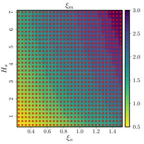
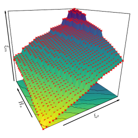
Figure 5: 2D coastal flooding application. (Left) 2D visualization of the $\xi_{m}$ values measured over a regular grid. (Right) 3D visualization of the $\xi_{m}$ data.

3.3.1 2D application

The coastal study site is located on a lido, which has faced two flood events in the past (Rohmer and Idier, 2012). The dataset used here contains 900 observations of the maximum water level at the coast $\xi_{m}$ depending on two input parameters: the offshore water level ($\xi_{o}$) and the wave height ($H_{s}$), both in metre units. The observations are taken within the domains $\xi_{o}\in[0.25,1.50]$ and $H_{s}\in[0.5,7]$ (with each dimension being discretized in 30 elements). One must note that, on the domain considered for the input variables, $\xi_{m}$ increases as $\xi_{o}$ and $H_{s}$ increase (see Figure 5).

Here, we normalised the input space to be in $[0,1]^{2}$. As covariance function, we used the tensor product of 1D SE kernels,

$$k_{\bm{\theta}}(\bm{x},\bm{x}^{\prime})=\sigma^{2}\exp\Big{\{}-{\frac{(x_{1}-x^{\prime}_{1})^{2}}{2\ell_{1}^{2}}}\Big{\}}\exp\Big{\{}-{\frac{(x_{2}-x^{\prime}_{2})^{2}}{2\ell_{2}^{2}}}\Big{\}},$$

with covariance parameters $\bm{\theta}=(\sigma^{2},\ell_{1},\ell_{2})$. Both $\bm{\theta}$ and the noise variance $\tau^{2}$ are estimated via ML. For the constrained model, we proposed emulators accounting for both positivity and monotonicity constraints, and we manually fixed the number of knots $m_{1}=m_{2}=25$ aiming a trade-off between high quality of resolution and computational cost.

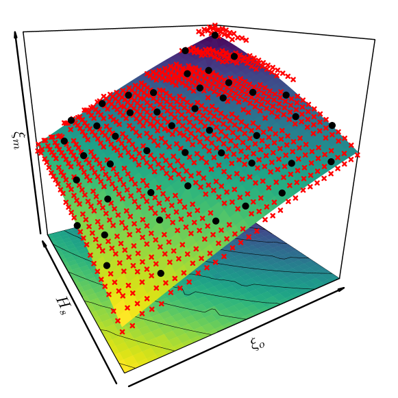
(a) Unconstrained GP: $Q^{2}=0.987$

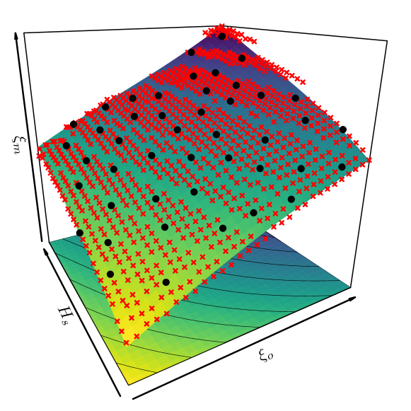
(b) Constrained GP: $Q^{2}=0.991$

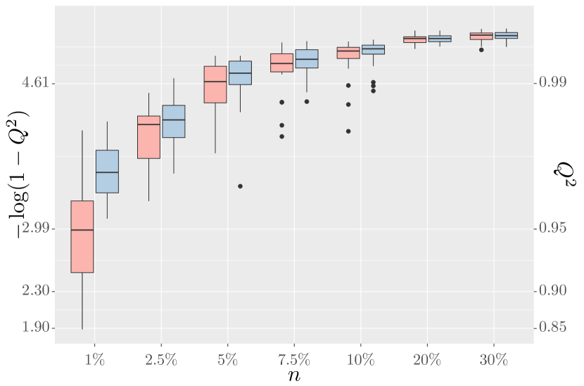
(c) $Q^{2}$ performance

Figure 6: 2D GP emulators for modelling the coastal flooding data in (Rohmer and Idier, 2012). (Left) Prediction results using 5% of the dataset via maximin Latin hypercube DoE. Each panel shows: training and test points (black dots and red crosses), the conditional mean function (solid surface), and the $Q^{2}$ criterion (subcaptions). 6(c) $Q^{2}$ assessment using different proportions of training points $n$ and using twenty different random training sets. Results are shown for the unconstrained (red) and constrained (blue) GP emulators.

For illustrative purposes, we first train both unconstrained and constrained GP emulators using 5% of the data (equivalent to 45 training points chosen by a maximin Latin hypercube DoE), and we aim at predicting the remaining 95%. Results are shown in Figures 6(a) and 6(b). In particular, one can observe that the constrained GP emulator slightly outperformed the prediction around the extreme values of $\xi_{m}$, leading to an absolute improvement of $4\%$ of the $Q^{2}$ indicator. Then, we repeat the experiment using twenty different sets of training data and different proportions of training data. According to Figure 6(c), one can observe that the constrained emulator often outperforms the unconstrained one, with significant $Q^{2}$ improvements for small training sets. As coastal flooding simulators are commonly costly-to-evaluate, the benefit of having accurate prediction with lesser number of observations becomes useful for practical implementations.

3.3.2 5D application

As in (Azzimonti et al., 2019), here we focus on the coastal flooding induced by overflow. We consider the “Boucholeurs” area located close to “La Rochelle”, France. This area was flooded during the 2010 Xynthia storm, an event characterized by a high storm surge in phase with a high spring tide. We focus on those primary drivers, and on how they affect the resulting flooded surface. We refer to (Azzimonti et al., 2019) for further details.

The dataset contains 200 observations of the flooded area $Y$ in $m^{2}$ depending on five input parameters $\textbf{x}=(T,S,\phi,t_{+},t_{-})$ detailing the offshore forcing conditions:

• The tide is simplified by a sinusoidal signal parametrised by its high tide level $T\in[0.95,3.70]$ ($m$).

• The surge signal is described by a triangular model using four parameters: the peak amplitude $S\in[0.65,2.50]$ ($m$), the phase difference $\phi\in[-6,6]$ (hours), between the surge peak and the high tide, the time duration of the raising part $t_{-}\in[-12.0,-0.5]$ (hours), and the falling part $t_{+}\in[0.5,12.0]$ (hours).

The dataset is freely available in the R package profExtrema (Azzimonti, 2018). One must note that the flooded area $Y$ increases as $T$ and $S$ increase.

Before implementing the corresponding GP emulators, we first analysed the structure of the dataset. We tested various standard linear regression models in order to understand the influence of each input variable $\textbf{x}=(T,S,\phi,t_{+},t_{-})$. We assessed the quality of the linear models using the adjusted $R^{2}$ criterion. Similarly to the $Q^{2}$ criterion, the $R^{2}$ indicator evaluates the quality of predictions over all the observation points rather than only over the training data. Therefore, for noise-free observations, the $R^{2}$ indicator is equal to one if the predictors are exactly equal to the data. We also tested various models considering different input variables (e.g. transformation of variables, or inclusion of interaction terms). After testing different linear models, we observed that they were more sensitive to the inputs $T$ and $S$ rather than to other ones. We also noted that, by transforming the phase coordinate $\phi\mapsto\cos(2\pi\phi)$, an absolute improvement about 26% of the $R^{2}$ indicator was obtained, and the influence of both $t_{-}$ and $t_{+}$ becomes more significant. Finally, we used these settings for the GP implementations.

We normalised the input space to be in $[0,1]^{5}$, and we used a covariance function given by the Kronecker product of 1D Matérn 5/2 kernels. The covariance parameters $\bm{\theta}=(\sigma^{2},\ell_{1},\cdots,\ell_{5})$ and the noise variance $\tau^{2}$ were estimated via ML. We also tested other types of kernel structures, including SE and Matérn 3/2 kernels, but less accurate predictions were obtained according to the $Q^{2}$ criterion. For the constrained model, we proposed GP emulators accounting for positivity constraints everywhere. We also imposed monotonicity constraints along the $T$ and $S$ input dimensions. Since the computational complexity of the constrained GP emulator increases with the number of knots $m$ used in the piecewise-linear representation, we strategically fixed them in coordinates requiring high quality of resolution. Since we observed that the contribution of the inputs $T$, $S$, $t_{-}$ and $t_{+}$ was almost linear (result in agreement with Azzimonti et al., 2019), we placed fewer number of knots over those entries. In particular, we fixed as number of knots per dimension: $m_{1}=m_{2}=4$, $m_{3}=5$ and $m_{1}=m_{2}=3$.

As in Section 3.3.1, we trained GP emulators using twenty different sets of training data and different proportions of training data. According to Figure 7, one can observe once again that the constrained GP emulator often outperforms the unconstrained one, with significant $Q^{2}$ improvements for small training sets. In particular, one can note that, by enforcing the GP emulators with both positivity and monotonicity constraints, accurate predictions were also provided by using only 10% of the observations as training points (equivalent to 20 observations).

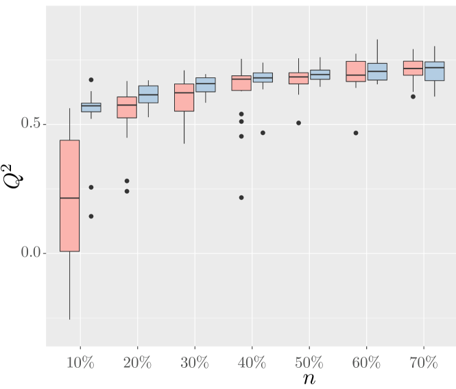
Figure 7: 5D GP emulators for modelling the coastal flooding data in (Azzimonti et al., 2019). The boxplots show the $Q^{2}$ results using different proportions of training points $n$ and using twenty different random training sets. Results are shown for the unconstrained (red) and constrained (blue) GP emulators.

4 Conclusions

We have introduced a constrained GP emulator with linear inequality conditions and noisy observations. By relaxing the interpolation of observations through a noise effect, MC and MCMC samplers are performed in less restrictive sample spaces. This leads to faster emulators while preserving high effective sampling rates. As seen in the experiments, the Hamiltonian Monte Carlo sampler from (Pakman and Paninski, 2014) usually outperformed its competitors, providing much more efficient effective sample rates in high dimensional sample spaces.

Since there is no need of having more knots than observations ($m\geq n$), the computational complexity of MC and MCMC samplers is independent of $n$. Therefore, since the samplers are performed on $\mathbb{R}^{m}$, they can be used for large values of $n$ by letting $m\ll n$. As shown in the 5D monotonic example, effective monotone emulations can be obtained within reasonable running times (about tens of minutes).

Despite the improvements obtained here for scaling the monotonic GP emulator in higher dimensions, its tensor structure makes it impractical for tens of input variables. We believe that this limitation could be mitigated by using other types of designs of the knots (e.g. sparse designs). In addition, supplementary assumptions on the nature of the target function can also be made to reduce the dimensionality of the sample spaces where MC and MCMC samplers are performed (e.g. additivity).

References

- Azzimonti (2018) Azzimonti, D. (2018). profExtrema: Compute and visualize profile extrema functions. https://cran.r-project.org/web/packages/profExtrema/index.html.
- Azzimonti et al. (2019) Azzimonti, D., Ginsbourger, D., Rohmer, J., and Idier, D. (2019). Profile extrema for visualizing and quantifying uncertainties on excursion regions. Application to coastal flooding. Technometrics, 0(ja):1–26.
- Bay et al. (2016) Bay, X., Grammont, L., and Maatouk, H. (2016). Generalization of the Kimeldorf-Wahba correspondence for constrained interpolation. Electronic journal of statistics , 10(1):1580–1595.
- Bishop (2007) Bishop, C. M. (2007). Pattern Recognition And Machine Learning (Information Science And Statistics). Springer.
- Botev (2017) Botev, Z. I. (2017). The normal law under linear restrictions: simulation and estimation via minimax tilting. Journal of the Royal Statistical Society: Series B (Statistical Methodology), 79(1):125–148.
- Cousin et al. (2016) Cousin, A., Maatouk, H., and Rullière, D. (2016). Kriging of financial term-structures. European Journal of Operational Research, 255(2):631–648.
- Deville et al. (2015) Deville, Y., Ginsbourger, D., Roustant, O., and Durrande, N. (2015). kergp: Gaussian Process Models with Customised Covariance Kernels. https://cran.r-project.org/web/packages/kergp/index.html.
- Dupuy et al. (2015) Dupuy, D., Helbert, C., and Franco, J. (2015). DiceDesign and DiceEval: Two R packages for design and analysis of computer experiments. Journal of Statistical Software, 65(i11).
- Geyer (1992) Geyer, C. J. (1992). Practical Markov Chain Monte Carlo. Statistical Science, 7(4):473–483.
- Golchi et al. (2015) Golchi, S., Bingham, D. R., Chipman, H., and Campbell, D. A. (2015). Monotone emulation of computer experiments. SIAM/ASA Journal on Uncertainty Quantification, 3(1):370–392.
- Goldfarb and Idnani (1982) Goldfarb, D. and Idnani, A. (1982). Dual and primal-dual methods for solving strictly convex quadratic programs. In Hennart, J. P., editor, Numerical Analysis, pages 226–239, Berlin, Heidelberg. Springer Berlin Heidelberg.
- Gong and Flegal (2016) Gong, L. and Flegal, J. M. (2016). A practical sequential stopping rule for high-dimensional Markov Chain Monte Carlo. Journal of Computational and Graphical Statistics, 25(3):684–700.
- Lan and Shahbaba (2016) Lan, S. and Shahbaba, B. (2016). Sampling Constrained Probability Distributions Using Spherical Augmentation, pages 25–71. Springer International Publishing, Cham.
- Larson and Bengzon (2013) Larson, M. G. and Bengzon, F. (2013). The Finite Element Method: Theory, Implementation, and Applications. Springer Publishing Company, Incorporated.
- López-Lopera (2018) López-Lopera, A. F. (2018). lineqGPR: Gaussian process regression models with linear inequality constraints. https://cran.r-project.org/web/packages/lineqGPR/index.html.
- López-Lopera et al. (2018) López-Lopera, A. F., Bachoc, F., Durrande, N., and Roustant, O. (2018). Finite-dimensional Gaussian approximation with linear inequality constraints. SIAM/ASA Journal on Uncertainty Quantification, 6(3):1224–1255.
- Maatouk and Bay (2016) Maatouk, H. and Bay, X. (2016). A New Rejection Sampling Method for Truncated Multivariate Gaussian Random Variables Restricted to Convex Sets, pages 521–530. Springer International Publishing, Cham.
- Maatouk and Bay (2017) Maatouk, H. and Bay, X. (2017). Gaussian process emulators for computer experiments with inequality constraints. Mathematical Geosciences, 49(5):557–582.
- Murphy (2012) Murphy, K. P. (2012). Machine Learning: A Probabilistic Perspective (Adaptive Computation And Machine Learning Series). The MIT Press.
- Pakman and Paninski (2014) Pakman, A. and Paninski, L. (2014). Exact Hamiltonian Monte Carlo for truncated multivariate Gaussians. Journal of Computational and Graphical Statistics, 23(2):518–542.
- Press et al. (1992) Press, W. H., Teukolsky, S. A., Vetterling, W. T., and Flannery, B. P. (1992). Numerical Recipes in C (2Nd Ed.): The Art of Scientific Computing. Cambridge University Press, New York, NY, USA.
- Rasmussen and Williams (2005) Rasmussen, C. E. and Williams, C. K. I. (2005). Gaussian Processes for Machine Learning (Adaptive Computation and Machine Learning). The MIT Press.
- Rohmer and Idier (2012) Rohmer, J. and Idier, D. (2012). A meta-modelling strategy to identify the critical offshore conditions for coastal flooding. Natural Hazards and Earth System Sciences, 12(9):2943–2955.
- Roustant et al. (2012) Roustant, O., Ginsbourger, D., Deville, Y., et al. (2012). DiceKriging, DiceOptim: Two R packages for the analysis of computer experiments by Kriging-based metamodeling and optimization. Journal of Statistical Software, 51(i01).
- Taylor and Benjamini (2017) Taylor, J. and Benjamini, Y. (2017). RestrictedMVN: multivariate normal restricted by affine constraints. https://cran.r-project.org/web/packages/restrictedMVN/index.html. [Online; 02-Feb-2017].