Chaos in time delay systems, an educational review

Abstract

The time needed to exchange information in the physical world induces a delay term when the respective system is modeled by differential equations. Time delays are hence ubiquitous, being furthermore likely to induce instabilities and with it various kinds of chaotic phases. Which are then the possible types of time delays, induced chaotic states, and methods suitable to characterize the resulting dynamics? This review presents an overview of the field that includes an in-depth discussion of the most important results, of the standard numerical approaches and of several novel tests for identifying chaos. Special emphasis is placed on a structured representation that is straightforward to follow. Several educational examples are included in addition as entry points to the rapidly developing field of time delay systems.

1 Introduction

The field of dynamical systems characterized by retarded interactions and time delays is rapidly developing. New concepts have been emerging in the last years together with an increasing palette of applications and tools to analyze field data. Against this backdrop we present here a review focusing in particular on recent developments and readability. Aiming to make the review accessible also to newcomers in the field we supplement selected concepts with basic educational examples.

1.1 Time delays in theory and nature

Dynamical systems with time delays are present in many fields [1], including engineering, mathematics, biology, ecology and physics. Especially well studied are optoelectronic circuits and laser coupled systems [2, 3], which may be considered to be model systems for delayed interactions. A range of novel phenomena have emerged in the past two decades from both extensive theoretical modeling efforts and experimental studies. Examples are the implementation of echo-state networks via the time sequencing of a single non-linear optical element with time delayed feedback [4], the optoelectronic realization of multi-stable delay systems, i. e. of systems with coexisting attractors [5], noise-induced resonances in delayed feedback systems [6], neuronal oscillations in feedforward delay networks [7], and the discovery of anticipating chaotic synchronization in autonomous [8, 9] and driven systems [10]. Delayed feedback is employed moreover for the control of chaotic [11, 12] and of noise-induced dynamics [13]. It has been furthermore shown that multistability can arise from delay coupling [14, 15].

Systems with constant time delays have been especially well studied, in part due to the precise timing capabilities of optoelectronics systems and lasers. Recent work addresses also non-constant time delays, which are known to be core to the dynamics of biological systems [16], such as for the brain [17, 18, 19], but which can be relevant also for photonic systems [20].

Turning and milling processes have become alternative prototype systems for the study of the impact of time delays [21, 22], in particular in relation to the question of how to control nonlinear delay systems [23]. The vibrations of the tool cutting a rotating workpiece during milling can be modeled incorporating constant time delays [24], time-varying delays [25], or a retardation depending on the state of the workpiece [21], viz of the dynamical system, with the latter allowing for an efficient suppression of vibrations [25].

For comparatively simple mechanical systems, such as the stick-balancing task [26, 27, 28], the influence of different types of delay have been studied extensively. The analysis of more complex systems, like climate models, for which the interaction of the atmosphere and the ocean may be characterized by distinct types of time-varying and/or state-dependent time delays, is in contrast substantially more demanding [29].

Besides a variety of new systems and time delay induced phenomena, novel methods and classification schemes for time delay dynamics have been proposed. Examples are partially predictable chaotic motion, as it can be found in delayed and classical dynamics systems [30], and a type of laminar chaos inherent to certain delay systems [31], with the latter being closely related to a specific classification of time-varying delays in terms of conservative and dissipative delays [32]. A novel spatio-temporal representation of delay systems allows furthermore for an interpretation in analogy to one-dimensional spatially extended systems [33], and as such for an intuitive understanding of delayed dynamics [34, 35].

1.2 Outline

For the groundwork we present in Sect. 1.3 a formal definition of time delay systems, and of the respective configuration and phase spaces, which will be followed in Sect. 1.4 by a discussion of the distinct ways local and global Lyapunov exponents may be defined for delay systems. The introduction then concludes with an educational analysis of the stability of fixed points in delay systems, for which several approaches to evaluate Lyapunov spectra are compared. Sect. 2 and 3 are then devoted respectively to comprehensive overviews of the most important types of time delay systems and of the dynamics, with the numerical methods being treated in Sect. 4.

1.3 States and state histories

A comprehensive class of delay differential equations are of the form

$$\dot{x}(t) =F\big{(}x(t),x(t-\tau)\big{)}\,,$$ (1)

where $\tau$ is the delay and $x$ a state in configuration space. To simplify the discussion, most definitions and examples presented throughout this review are given, as for (1), for systems characterized by a single scalar variable $x$ and a single constant time delay $\tau$.

The trajectories of a delay differential equation (DDE) such as (1) are uniquely defined by their associated initial functions $\varphi(t)$ on an initial time interval,

$$x(t)=\varphi(t),\qquad\quad t\in[t_{\text{o}}-\tau,t_{\text{o}}]\,.$$ (2)

Delay differential equations (DDE) are, as a consequence, formally infinite dimensional. A state in phase space is hence not uniquely determined by $x=x(t)$, but by the state history

$$\mathbf{X}(t) =\{x(t^{\prime})\}\,,\qquad\quad t^{\prime}\in[t-\tau,t]\,.$$ (3)

In analogy we define the directed distance vector $\mathbf{d}(t)$ between two state histories as

$$\mathbf{d}(t) =\mathbf{X}_{1}(t)-\mathbf{X}_{\text{o}}(t)$$ (4)

$$=\{x_{1}(t^{\prime})-x_{\text{o}}(t^{\prime})\}\,,\qquad\quad t^{\prime}\in[t-\tau,t]\,,$$

with the respective norm $d=d(t)$ being

$$d(t) =\left(\frac{1}{\tau}\int_{t-\tau}^{t}\!\!\mathrm{d}t^{\prime}\;\lvert x_{1}(t^{\prime})-x_{\text{o}}(t^{\prime})\rvert^{\gamma}\right)^{1/\gamma}\,,$$ (5)

where $\gamma=2$ for a Euclidean metric. For $\gamma=1$ one has the Manhattan norm, which corresponds to the average distance between two trajectories, when averaging over a time interval $\tau$. We will work here with a Euclidean space of state histories.

1.4 Lyapunov exponents

The classical definition of Lyapunov exponents, as established for ordinary dynamical systems, can be generalized to time delay systems. We distinguish here between local Lyapunov exponents $\Lambda_{j}\in\mathbb{C}$ [36, 37], which are complex numbers, and real-valued global Lyapunov exponents $\lambda_{j}\in\mathbb{R}$ [38, 36], among which the largest one, the maximal (global) Lyapunov exponent $\lambda_{\text{max}}$ is of particular interest. Futher, note that the finite-time Lyapunov exponents (cf. Sect. 4.2.2) are different from local Lyapunov exponents.

1.4.1 Local Lyapunov exponents

For the local stability of a DDE (1) one considers the time evolution of a small perturbation $\delta$ (see also Sect. 3.1)

$$\dot{\delta}(t)=J_{\text{o}}\,\delta(t)+J_{\tau}\,\delta(t-\tau)\,.$$ (6)

Here we have denoted with $J_{\text{o}}$ the instantaneous Jacobian and with $J_{\tau}$ the delayed Jacobian, which are defined by the partial derivatives of the flow $F$ with respect to the instantaneous and the delayed state, respectively [39]:

$$J_{\text{o}}=\frac{\partial F\big{(}x(t),x(t-\tau)\big{)}}{\partial x(t)},\quad\qquad J_{\tau}=\frac{\partial F\big{(}x(t),x(t-\tau)\big{)}}{\partial x(t-\tau)}\,.$$ (7)

Here, the Jacobians $J_{\text{o}},J_{\tau}$ are scalar quantities, as we only consider scalar systems (1), i. e. $x\in\mathbb{R}$. For DDE in $N$ dimensions, the Jacobians are $N\times N$ matrices. Note that both Jacobians depend on the actual state $x(t)$ and on the delayed state $x(t-\tau)$ of the system.

In the case of ordinary differential equations (ODE), i. e. without delay $\tau=0$, $J_{\tau}=0$, the $N$, generally complex eigenvalues of the Jacobian $J_{\text{o}}$ are termed local Lyapunov exponents. For a one-dimensional ODE, the instantaneous Jacobian $J_{\text{o}}\in\mathbb{R}$ coincides with the only local Lyapunov exponent. One may study local Lyapunov exponents anywhere in phase space, even though they are typically used to classify fixed points as foci, saddles and nodes [40].

In order to generalize the concept of local Lyapunov exponents $\Lambda_{j}$ for finite delays $\tau>0$, one may approximate any DDE by a finite-dimensional Euler map (see Sect. 4.2.3). Then the local Lyapunov exponents $\Lambda_{j}$ of the DDE can be estimated at every point in the phase space of the delayed system from the eigenvalues of the map’s Jacobian matrix. As a special case one may, on the other hand, directly evaluate the local Lyapunov exponents for the delayed system at a fixed point of DDE (1) via a characteristic equation (see Sect. 3.1) [39, 36]. Note that we do not use the term local Lyapunov exponents to refer to finite-time Lyapunov exponents (cf. Sect. 1.4.2).

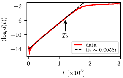
Figure 1: The logarithmic distance $\log(d)$ between two trajectories of the Mackey-Glass system (cf. Sect. 2.1), for $\tau=17.20$ and averaged over $100$ pairs with initial distance $\delta=10^{-6}$. The slope of the linear fit (dashed line) retrieves the maximal Lyapunov exponent $\lambda_{\text{max}}=0.0058$ as defined by Eq. (8). The Lyapunov prediction time $T_{\lambda}=1071$, as defined in Sect. 3.4, is marked to indicate the average time it takes until the distance between a pair of trajectories has reached $d=10^{-2}$. Note that $\log 10^{-6}\approx-13.8$ and $\log 10^{-2}\approx-4.6$.

1.4.2 Global and maximal Lyapunov exponents

An initially small distance $\delta$ between two trajectories, as defined by (5), may be assumed to evolve exponentially,

$$d(t) =\delta\;\e^{\lambda_{\text{max}}t},\quad\qquad\lambda_{\text{max}}=\lim\limits_{t\to\infty}\lim\limits_{\delta\to 0}\frac{1}{t}\log\left(\frac{d(t)}{\delta}\right)\,,$$ (8)

which defines the largest Lyapunov exponent $\lambda_{\text{max}}$. Note that the limit of an infinitesimal small initial distance and an infinitely long divergence is subject to the constraint that overall distances are finite for bounded dynamical systems.

The formal definition (8) has been extended to the more general concept of finite-time Lyapunov exponents [41, 42], and finite-size Lyapunov exponents [43]. Lyapunov exponents may be extracted directly from data series [36], as illustrated in Fig. 1, where the initial slope of the logarithmic distance $\log(d)$ is used to approximate the maximal Lyapunov exponent $\lambda_{\text{max}}$.

The largest global Lyapunov exponent $\lambda_{\text{max}}=\lambda_{1}$ captures the rate of divergence in the direction of the fastest divergence of trajectories. Further Lyapunov exponents $\lambda_{j}$, with $j>1$, describe then the remaining directions. In a system with an infinite number of dimensions there is potentially an infinite number of distinct Lyapunov exponents $\lambda_{j}$, with the entirety being called the Lyapunov spectrum. It is common to order the exponents by size,

$$\lambda_{\text{max}}=\lambda_{1}\geq\lambda_{2}\geq\ldots\,.$$ (9)

Computationally the Lyapunov spectrum is computed in general resorting to Benettin’s method [44, 45, 46, 47], which will be detailed out in Sect. 4.2.2.

1.4.3 Global Lyapunov exponents for maps

As an alternative to the numerical treatment one may extract the Lyapunov spectrum (9) from the Euler map, which we will define in Sect. 4.1.2. For this approach one needs to know the time evolution operator $M(t)$ explicitly, a precondition holding for the Euler map and in general for discrete maps, for which $M(t)$ is given by a suitable product of the map’s Jacobian matrix [48].

We consider the distance vector $\mathbf{d}_{j}(t)$ between the state histories of two trajectories, $x_{\text{o}}(t)$ and $x_{j}(t)$, where $x_{\text{o}}(t)$ is a reference orbit. Neglecting mathematical subtleties [49, 38], one may assume that the time evolution of $\mathbf{d}_{j}(t)$ is governed by the time evolution operator,

$$\mathbf{d}_{j}(t) =M(t)\;\boldsymbol{\delta}_{j}\,,$$ (10)

where $\boldsymbol{\delta}_{j}=\mathbf{d}_{j}(0)$ is the vector corresponding to the initial distance $\delta$, which we take to be small. The norm of the distance vector can then be expressed with

$$\lVert\mathbf{d}_{j}(t)\rVert =\sqrt{\boldsymbol{\delta}_{j}^{\intercal}M^{\intercal}(t)M(t)\boldsymbol{\delta}_{j}}=\sqrt{\boldsymbol{\delta}_{j}^{\intercal}U(t)\boldsymbol{\delta}_{j}}$$ (11)

as a function of the matrix $U(t)=M^{\intercal}(t)M(t)$, where $M^{\intercal}$ and $\boldsymbol{\delta}_{j}^{\intercal}$ are the transpose of $M$, which is a matrix [50, 48], and respectively of $\boldsymbol{\delta}_{j}$. With $U$ being real and symmetric, its eigenvalues $\alpha_{j}(t)$ and the corresponding eigenvectors $\mathbf{e}_{j}$ are also real. One has furthermore that $\alpha_{j}(t)\geq 0$ holds, as

$$\lVert M\mathbf{e}_{j}\rVert^{2}=\mathbf{e}_{j}^{\intercal}M^{\intercal}M\mathbf{e}_{j}=\mathbf{e}_{j}^{\intercal}U\mathbf{e}_{j}=\alpha_{j}\lVert\mathbf{e}_{j}\rVert^{2}\,.$$ (12)

Choosing the $j$th eigenvector $\mathbf{e}_{j}$ of $U$ to be aligned with the initial distance $\boldsymbol{\delta}_{j}$ one then obtains

$$\lVert\mathbf{d}_{j}(t)\rVert =\sqrt{\alpha_{j}(t)}\;\lVert\boldsymbol{\delta}_{j}\rVert$$ (13)

for the evolution of the distance $\lVert\mathbf{d}_{j}(t)\rVert$ between two state histories. Using (8), we may then express the $j$th global Lyapunov exponent $\lambda_{j}$ in terms of the $j$th eigenvalue $\alpha_{j}(t)$ of $U(t)$:

$$\lambda_{j} =\lim\limits_{t\to\infty}\frac{\log\alpha_{j}(t)}{2t}\,.$$ (14)

This expression is useful when extracting Lyapunov exponents from the Euler map (cf. Sect. 1.5.2), as we will detail out in Sect. 4.2.3. Eq. (14) shows in particular that the spectrum of Lyapunov exponents is well defined.

1.5 Educational example: Stability of a fixed point

In order to discuss several notions related to the stability of a fixed point we consider with

$$\dot{x}(t) =-x(t-\tau)$$ (15)

the simplest time delay system [51]. The evolution of small perturbations around $x^{*}$ are determined by the local Lyapunov exponent, which depends in turn on the delay time $\tau$. The stability of the fixed point in terms of the Lyapunov exponent can be evaluated by the standard analytic ansatz, as discussed in the following Sect. 1.5.1, and via the Euler map (cf. Sect. 1.5.2). Numerical methods for the evaluation of both the maximal Lyapunov exponent and of the Lyapunov spectrum, such as the Benettin method [44], will be treated later in Sect. 4.2. Here we will use Benettin’s approach for benchmarking.

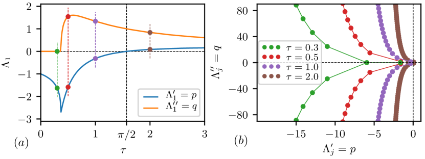
Figure 2: The spectrum of local Lyapunov exponents $\Lambda_{j}=\Lambda_{j}^{\prime}+\imath\Lambda_{\text{j}}^{\prime\prime}$ for the DDE (15) at the fixed point $x^{*}=0$ in terms of the roots of (19). Note that the spectrum is countably infinite. ($a$) Real and imaginary part (shown is one of the two branches) of the largest exponents $\Lambda_{1}$ as a function of the delay $\tau$. The real part changes sign at $\tau=\pi/2$ (vertical dashed line, cf. Eq. (18)). Bullets and vertical lines indicate the maximal local Lyapunov exponent of the spectra shown in the right-hand panel (colors matching). ($b$) The imaginary part $\Lambda_{\text{j}}^{\prime\prime}$ as a function of the real part $\Lambda_{j}^{\prime}$. Lines are guides to the eye.

1.5.1 Analytic ansatz for local Lyapunov exponents

Close to the fixed point $x^{*}=0$ the dynamics of (15) can be approximated by the exponential ansatz $x(t)\propto\exp(\Lambda t)$ for the complex local Lyapunov exponents $\Lambda_{j}=\Lambda_{j}^{\prime}+\imath\Lambda_{j}^{\prime\prime}\to\Lambda=p+\imath q$, where we drop the index and denote with $p=\Lambda_{j}^{\prime}$ the real part and with $q=\Lambda_{j}^{\prime\prime}$ the imaginary part (cf. Sect. 3.1). The characteristic equation is consequently [52]

$$\Lambda =-\e^{-\Lambda\tau},\qquad\quad\Lambda=p+\imath q\,,$$ (16)

which can be separated into a real and an imaginary part:

$$p=-\e^{-p\tau}\cos(q\tau),\qquad\quad q=\e^{-p\tau}\sin(q\tau)\,.$$ (17)

This equation has, as a graphical inspection shows, an infinite number of solutions, which we may order with respect to the real part: $p_{1}\geq p_{2}\geq\dots$. The fixed point is stable when $p_{1}<0$, viz when $\cos(q_{1}\tau)>0$. The transition occurs, as shown in Fig. 2, for

$$p_{1}=0,\quad\quad q_{1}=1,\quad\quad\tau=\pi/2,\quad\quad q_{1}\tau=\pi/2\,,$$ (18)

viz when the time delay $\tau$ starts to be out-of-phase with the period $2\pi/q$ of the Lyapunov oscillation. Eliminating $p$ from (17) one obtains the transcendental equation

$$q =\e^{q\tau/\tan(q\tau)}\sin(q\tau),\qquad\quad p=-q/\tan(q\tau)\,,$$ (19)

for the imaginary part $q$ of the local Lyapunov exponent. Note that (19) has a countable but infinite number of roots, the local Lyapunov spectrum, which can be found numerically, e. g., via bisection.

For any solution of Eq. (19) with non-vanishing imaginary part $q\neq 0$ there exists a complex conjugate solution – a necessary condition when $x=x(t)$ is real. Thus, the Lyapunov spectrum is symmetric with respect to the sign of the imaginary part, viz when interchanging $q\leftrightarrow(-q)$. In Fig. 2 the numerical solution of Eq. (19) for different values of the delay time $\tau$ are given.

All roots have negative real parts, $p<0$, when the delay is small, viz when $\tau<\pi/2$. The fixed point $x^{*}=0$ is then attracting. Above the transition $\tau=\pi/2$ at least one Lyapunov exponent is positive, with the number of positive exponents increasing with increasing delay $\tau$. The fixed point is then repelling.

In Fig. 3 the real part $\Lambda_{j}^{\prime}$ of the roots of (19) is shown in comparison with the Lyapunov exponents $\lambda_{j}$ obtained numerically using Benettin’s approach (cf. Sect. 1.4). One finds point per point agreement.

When the delay vanishes $\tau\to 0$ the DDE (15) turns into an ordinary differential equation (ODE) and the dimensionality of the system reduces from an infinite number of dimension to one dimension. In consequence the spectrum of local Lyapunov exponents $\Lambda_{j}$ collapses onto a single exponent $\Lambda_{1}=\partial\dot{x}/\partial x=-1$, which approaches its value from below when decreasing the delay. The real parts of the rest of the spectrum diverges with the second largest local Lyapunov exponent $\lim_{\tau\to 0}\Lambda_{2}=-\infty$ leading to a compactification of dimensions.

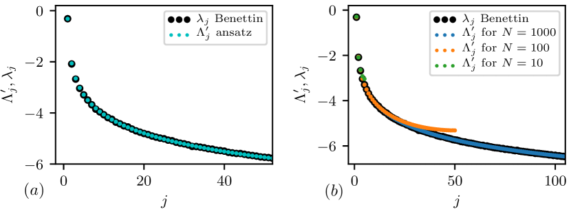
Figure 3: A comparison of methods determining the stability of the fixed point $x^{*}=0$ of the DDE (15) for $\tau=1$ (showing only values for non-negative imaginary parts $\Lambda_{j}^{\prime\prime},\lambda_{j}^{\prime\prime}\geq 0$). ($a$) The real part $\Lambda_{j}^{\prime}$ of the exponents solving (16) are in agreement with the Lyapunov exponents $\lambda_{j}$ computed with Benettin’s method (black bullets, cf. Sect. 4.2.2). ($b$) The real part $\Lambda^{\prime}_{j}$ of the (local) Lyapunov exponents, as estimated from the eigenvalues of the $N\times N$ Jacobian (26) of the Euler map (colored dots), in comparison with the Lyapunov exponents computed with Benettin’s method (black bullets). The agreement improves rapidly with increasing resolution $N$ of the Euler map.

1.5.2 Euler map

One may discretize time, such that the delay interval $\tau$ is subdivided into $N-1$ segments of length $\varDelta t$, as described in Sect. 4.2.3. A DDE is such transformed to a discrete map, the Euler map.

For Eq. (15) the $N\times N$ Jacobian matrix of the Euler map is given by

$$J =\left(\begin{array}[]{cccccc}-\varDelta t&0&\lx@intercol\hfil\cdots\hfil\lx@intercol&0&1\\ -\varDelta t&-\varDelta t&0&\cdots&0&1\\ \vdots&&\ddots&\ddots&\vdots&\vdots\\ \vdots&&\ddots&\ddots&0&\vdots\\ -\varDelta t&\lx@intercol\hfil\cdots\hfil\lx@intercol&&-\varDelta t&1\\ -\varDelta t&\lx@intercol\hfil\cdots\hfil\lx@intercol&-\varDelta t&1-\varDelta t\end{array}\right)\,,$$ (26)

where the steps size $\varDelta t=\tau/(N-1)$ depends on the resolution $N$. From the $N$, in general complex eigenvalues $\sigma_{j}$ of (26), one can estimate the real parts $\Lambda^{\prime}_{j}$ of the $N$ largest (local) Lyapunov exponents of (15). For this purpose one uses the relation (cf. Sect. 4.2.3)

$$\lVert\sigma_{j}\rVert^{2}=(\sigma_{j}^{\prime})^{2}+(\sigma_{j}^{\prime\prime})^{2}\to\e^{2\Lambda^{\prime}_{j}\tau}\quad\text{ for }N\to\infty\,$$ (27)

for the modulus of complex numbers, which follows from (14). From the relation of the complex eigenvalue $\sigma_{j}$ and the complex local Lyapunov exponent $\Lambda_{j}$,

$$\sigma_{j}^{\prime}+\sigma_{j}^{\prime\prime}\to\exp\Big{(}\tau\big{(}\Lambda_{j}^{\prime}+\imath\Lambda^{\prime\prime}_{j}\big{)}\Big{)}\,,$$ (28)

one can also extract the imaginary part $\Lambda_{j}^{\prime\prime}$ modulo $2\pi/\tau$ (cf. Sect. 4.2.3).

Fig. 3 shows the results for $\tau=1$ and a series of $N$, in comparison to the Lyapunov exponent obtained with the Benettin method (cf. Sect. 4.2.2). The largest Lyapunov exponents are approximated well even for a limited resolution $N\sim 10$.

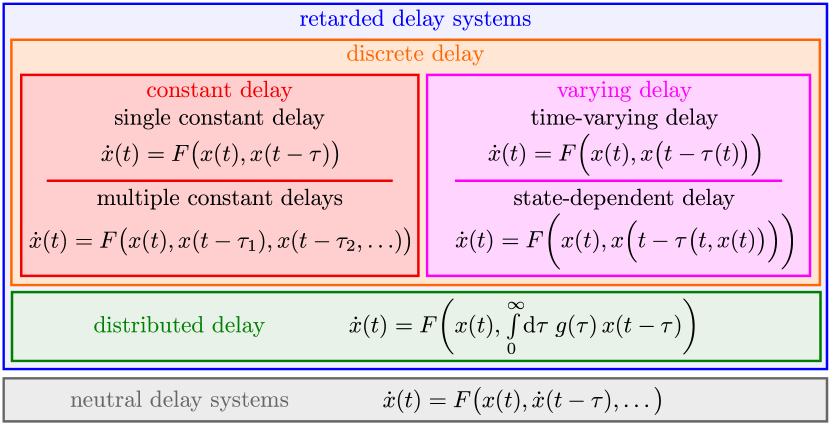
Figure 4: Overview and categorization of the different time delays discussed in Sect. 2.

2 Types of time delay systems

A large class of delay differential equations (DDE) take the form of a continuous-time dynamical system of the type

$$\dot{x}(t) =F\big{(}x(t),\alpha\big{)}\,,$$ (29)

where $x(t)\in\mathbb{R}$ denotes the state of the system parameterized by the time $t$. The flow $F\,:\,\mathbb{R}\times\mathbb{R}\to\mathbb{R}$ depends on the current state $x(t)$ and on a delay function $\alpha\in\mathbb{R}$, which we will specify later on for the distinct types of time delays For simplicity the DDE (29) is chosen to be scalar and the flow to be autonomous, with the latter implying that $F$ is not an explicit function of time. A summary of the most important types time delays is presented in Fig. 4.

2.1 Single constant time delay

The simplest but non-trivial delay function $\alpha=x(t-\tau)$ incorporates a single constant time delay $\tau>0$ [40]. The corresponding DDE depends then on a single past state:

$$\dot{x}(t) =F\big{(}x(t),x(t-\tau)\big{)}\,.$$ (30)

An example for this type of DDE has been discussed previously, see Eq. (15).

Single constant time delays are experimentally realized in optical laser systems [53], where they can be used to generate chaotic communication [54], that is communication channels suitable for private communication [55]. Examples of theoretical investigations using this type of DDE include the modeling of traffic dynamics by car-following models [56] and word recognition with time delayed neural networks [57].

A possible reference system for a DDE is the limit of vanishing time delay, viz the case $\alpha\to 0$ in (29). Systems with stable instantaneous evolution will become unstable, as illustrated in Fig. 2, when the length $\tau$ of the time delay becomes larger than the time scale of the instantaneous dynamics [40]. This observation has led to the suggestions that modern democracies may be generically unstable [58]. The instability would result in this context from the growing mismatch between the ongoing acceleration of the instantaneous political dynamics, as defined by the time scale of opinion swings, and a delayed feedback that is entrenched in the election cycle.

A reference example for a DDE with a delay induced instability is the Mackey-Glass system [59]:

$$\dot{x}(t) =\frac{a\,x(t-\tau)}{1+\big{(}x(t-\tau)\big{)}^{c}}-b\,x(t)~{}.$$ (31)

The typical choice for the parameters, $a=0.2$, $b=0.1$ and $c=10$, ensures that the trivial fixed point $x=0$ is unstable for all time delays [47] and that the non-trivial fixed point $(a/b-1)^{1/c}=1$ is stable for small time delays. Increasing the time delay $\tau$ one observes first periodic oscillations and then a transition to chaos [47]. Originally designed to describe the production of blood cells, the Mackey-Glass is now considered a standard example of deterministic chaos [60], for which it is widely used for bench marking results [61, 46, 62]. The Mackey-Glass system will serve in this review as a reference system for the discussion of chaos, as presented in Sect. 3.

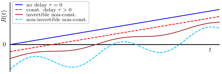
Figure 5: Illustration of selected continuous access functions $R(t)=t-\tau(t)$. An access function is non-invertible if $\dot{R}<0$.

2.2 Multiple constant time delays

For systems with multiple constant time delays $\tau_{1},\tau_{2},\ldots>0$ the delay function $\alpha=\alpha(x(t-\tau_{1}),x(t-\tau_{2}),\ldots)$ depends on several corresponding past states. Multiple constant time delays are used to study, e. g., synchronization properties in heterogeneous networks [63, 64]. Experimentally systems with multiple constant time delays are realized in coupled optoelectronic oscillators [53], where the combination of different time delays is used to create states of full or partial synchronization. In a modified Stuart-Landau model [65] two distinct time delays induce instabilities that exhibit spatio-temporal pattern formation and turbulence [66]. In time delay systems with state-switching the dynamics becomes more robust to noise, when two distinct time delays are incorporated [67].

The destabilization of a stationary state in systems with multiple constant delays can happen via different types of bifurcations [68]. It has been shown [69], on the other hand, that multiple time delay feedback may suppress chaotic dynamics in Chua’s circuit [70]. We note that chaos can be suppressed quite in general by stabilizing fixed points or by inhibiting noise modulations [71]. In addition we mention that an increase of the time delay leads to an improvement in the performance in act-and-wait feedback systems [72].

2.3 Time-varying delay

For time-dependent non-constant time delays $\tau=\tau(t)$ the delay differential equation reads

$$\dot{x}(t) =F\Big{(}x(t),x\big{(}R(t)\big{)}\Big{)}\,,\qquad\quad R(t)=t-\tau(t)\,,$$ (32)

where we have defined with $R(t)$ the access function (or access map [32]). Discontinuous or non-invertible access functions are generically not considered. Periodically varying delays [73, 31], like a sinusoidal variation

$$\tau(t) =\tau_{\text{o}}+A\sin(\omega t)$$ (33)

with mean $\tau_{\text{o}}$ and amplitude $A$, become non-invertible whenever $|A\omega|>1$. An example is shown in Fig. 5. Periodic time delays may be used to stabilize systems that are strongly chaotic in the limit of fixed time delay, viz when $A\to 0$. In general, a periodically varying delay is incorporated to non-linear delayed feedback in order to study the effect on synchronization [74] or on chaotic behavior [75]. Implemented in electronic circuits, periodically varying delay have been shown to stabilize unstable orbits [76].

The dynamics of stochastically varying time delays [77],

$$\tau(t) =\tau_{\text{o}}+\int\limits_{0}^{t}\mathrm{d}t^{\prime}\,\xi(t^{\prime})\,,$$ (34)

can be characterized on the other hand only by statistical distributions. The stochastic process is described by the random variable $\xi(t)$ generating the noise distribution. Noise may prevent the collapse of phase-space trajectories onto simple manifolds [77, 55], as observed regularly for systems with fixed time delays (cf. Sect. 3.2.2 on partially predictable chaos). This effect is illustrated in Fig. 6 for the Mackey-Glass system (31). Stochastically time-varying delays are used in control schemes for communication networks [78] and for tuning fuzzy PID controllers [79]. It has been shown moreover that the distribution of stochastically varying delay has an impact on the stability of the dynamics [80].

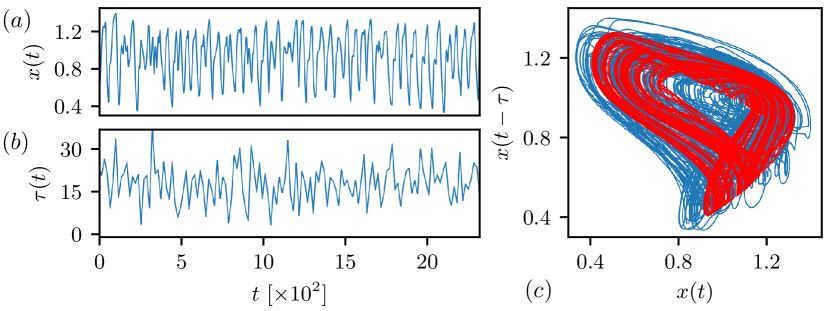
Figure 6: The Mackey-Glass system (31) with stochastically varying time delay (34). ($a$) Chaotic time series $x(t)$ and ($b$) stochastic time delay $\tau(t)$ with mean $\mu_{\tau}=\tau_{\text{o}}=17.20$ and variance $\sigma_{\tau}=7$ over time. ($c$) Attractors in the $x(t)$, $x(t-\tau)$ projection with varying delay (blue, cf. panels ($a,b$)) and fixed time delay $\tau=\tau_{\text{o}}$ (red). Figure replicated from [77].

In systems with digital controllers the controlled signals are measured at discrete times and with finite precision, a strategy called digital sampling [81]. Modern control systems belong mostly to this class of time delay systems. With digital sampling the state of the system is detected with a certain sampling period, inducing a time-dependent delay between the controlled system and the digital controller, which may in turn be expressed in terms of a discrete mapping [82]. For systems with differential control it has been shown that digital sampling can exhibit micro-chaos [82], which manifests itself as chaotic vibrations on comparably small length scales in the controlled system. Micro-chaos can be permanent or appear transiently [83].

2.4 State-dependent delay

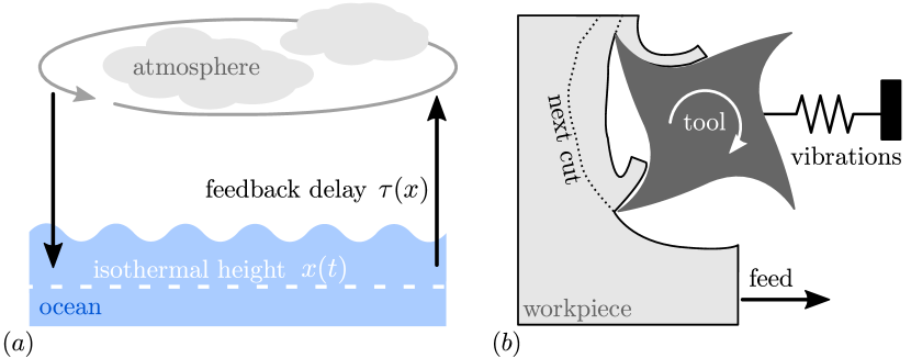
Figure 7: Examples of systems with state-dependent time delay. ($a$) Sketch of the interacting dynamics between the ocean and the atmosphere. The delay in the feedback mechanism depends on the internal state of the atmosphere or the ocean, e. g. on the isothermal height $x(t)$ of the ocean. Figure inspired by [29]. ($b$) Mechanical model for describing the cutting processes with a vibrating tool. The edge cut by the tool into the workpiece depends on the edge of the previous cut, which makes the delay state dependent. Figure inspired by [21].

The feedback mechanism generating time delays in physical systems may depend on the state of the system itself [84]. A non-constant state-dependent time delay $\tau(t,x(t))$,

$$\dot{x}(t) =F\bigg{(}x(t),x\Big{(}t-\tau\big{(}t,x(t)\big{)}\Big{)}\bigg{)}$$ (35)

may then result. This type of time delay can be considered as an additional dimension to the dynamical system, adding further to the complexity.

In the DAO (Delayed Action Oscillator) paradigm of the ENSO (El Ni$\tilde{\mbox{n}}$o Southern Oscillation) climate model [29], the delay induced by the mutual feedback mechanism of ocean and atmosphere depends on the physical state of either part of the system, see Fig. 7.

Time delay systems with state-dependent delays are employed in control tasks, such as the balancing of an inverted pendulum with a PD controller [27], or when modeling milling processes [21] (cf. Fig. 7). Due to the vibrations of workpiece and tool, the chip thickness and shape of each cut of the tool depends on the previous cut, which makes milling processes with vibrations [21], and turning processes [85], prototype systems for state-dependent delays. Besides numerical simulations only few universal analytic results, such as a rigorous theory for linearizing state-dependent DDE [86], are known for state-dependent delays.

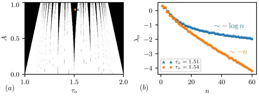
Figure 8: ($a$) Parameter space of a periodically varying time delay (33) with amplitude $A$ and mean $\tau_{\text{o}}$. In the black regions the delay is dissipative, whereas it is conservative in the white regions. The two regions in parameter space are separated by fractal Arnold tongues. ($b$) Lyapunov spectra $\lambda_{n}$ of an attractor in a time delay systems with periodically varying time delay (33) (cf. Sect. 3.2.4, see [87, 32]). Shown is the spectrum for a conservative (blue triangles, $\tau_{\text{o}}=1.51,A=0.9$) and a dissipative (orange bullets, $\tau_{\text{o}}=1.54,A=0.9$) time delay. For the first the asymptotic scaling of the spectrum is logarithmic $\lambda_{n}\sim-\log n$, for the latter it is linear $\lambda_{n}\sim-n$. Figures replicated from [87].

2.5 Conservative vs. dissipative delay

It has been proposed that state-dependent time delays may be classified to be either conservative or dissipative [87, 32]. For invertible access maps $R(t)=t-\tau(x(t),t)$ (see Fig. 5), a transformation $\Phi(t)=\varphi$ of the time scale $t\to\varphi$ leads to a corresponding transformation of the access function $R(t)\to\tilde{R}(\varphi)$:

$$\tilde{R}(\varphi) =\Phi\,R(t)\,\Phi^{-1},\qquad\quad t\to\varphi=\Phi(t)\,.$$ (36)

If the transformed access map $\tilde{R}(\varphi)=\varphi-\tau_{\varphi}$ is equivalent to the access map for a constant delay $\tau_{\varphi}>0$, then the delay is considered to be conservative [32], otherwise it is said to be dissipative. Conservative time delays are known under various names in different fields: Within engineering conservative delays are called variable transport delays [88, 89], whereas they are referred to as threshold delays in biological systems [90, 91].

For periodically varying time delay (cf. Eq. (33)), the dissipative and conservative regions in parameter space are fractionally divided by Arnold tongues (cf. Fig. 8). The mapping of time instances $t_{n}$ defined by the access function $R(t)$

$$t_{n+1} =R(t_{n})=t_{n}-\tau(t_{n})$$ (37)

is equivalent to a circle map [87], when using sinusoidally varying time delays (33), with dissipative time delays corresponding to chaotic behavior of the circle map (37).

Conservative systems, which are equivalent to systems with a constant time delay [89], tend to be less complex than dissipative systems, for which a new type of chaotic motion, laminar chaos [31], has been found. See Sect. 3.2.4. The two classes differ furthermore with respect to the scaling of the Lyapunov spectrum, which we will define in Sect. 1.4. The well studied logarithmic scaling of the Lyapunov exponents $\lambda_{n}\sim-\log n$ for $n\to\infty$ holds for conservative delays [47], as depicted in Fig. 8. For dissipative delays a linear scaling $\lambda_{n}\sim-n$ is observed in contrast [32].

2.6 Distribution of delays

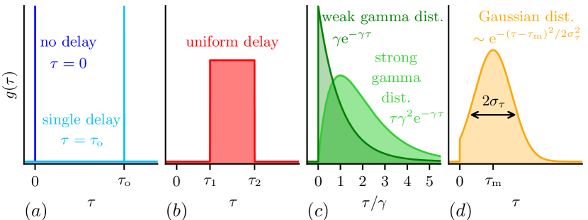
Figure 9: Different distributions $g(\tau)$ of delays $\tau\geq 0$. ($a$) Dirac delta delay distributions are equivalent to single constant delays. ($b$) Uniform distribution of delay in the range $[\tau_{1},\tau_{2}]$ with height $1/(\tau_{2}-\tau_{1})$. ($c$) Two examples of gamma distributions characterized by the parameter $\gamma>0$: the weak gamma distribution, which decays exponentially, and the strong gamma distribution, as characterized by a pronounced contribution around $\tau=1/\gamma$. ($d$) A Gaussian with mean $\tau_{\text{m}}$ and variance $\sigma_{\tau}^{2}$.

The discussion concerned hitherto discrete delays, that is systems for which the evolution of the current state is influenced by distinct instances of the past. This is a valid approximation for, e. g., optical systems, for which there is only little variation of the delay. However, biological [16] and social [58] systems may be described more accurately by time delays that are drawn from a probability distribution $g(\tau)$,

$$g(\tau)\geq 0\,,\qquad\int\limits_{0}^{\infty}\mathrm{d}\tau\;g(\tau) =1\,,\qquad g(\tau\!<\!0)=0\,,$$ (38)

of delays. The distribution vanishes for the sake of causality for negative delays.

A distribution of time delays may enter in two ways. For the first possibility the dynamics as such is averaged over the distribution of time delays:

$$\dot{x}(t)=\int\limits_{0}^{\infty}\mathrm{d}\tau\,g(\tau)F\big{(}x(t),x(t-\tau)\big{)}\,.$$ (39)

For a non-linear bare flow $F$ the delay differential equation is in this case not of the form given by Eq. (29).

A more common way to incorporate a distribution of delays is to assume that the dynamics is influenced solely by a weighted average $\alpha$ of past states:

$$\dot{x}(t) =F\big{(}x(t),\alpha\big{)},\qquad\quad\alpha=\int\limits_{0}^{\infty}\!\mathrm{d}\tau\,g(\tau)\,x(t-\tau)\,.$$ (40)

The two approaches, (39) and (40), coincide for linear dynamics. The standard stability analysis of fixed points (cf. Sect. 1.5.1) can be carried out also for distributed time delays [58], with the investigation being particularly straightforward for a $g(\tau)$ which can be Laplace-transformed analytically [92].

A selection of delay distributions is presented in Fig. 9. Dirac delta functions correspond to fixed time delays and uniform time delay distributions to the flat average over a past time interval $[t-\tau_{1},t-\tau_{2}]$ (cf. Fig. 9). The latter has been employed for describing the aging transition of a delay coupled network of oscillators [92] and for the delayed influences within advanced political systems. [58]. Note, that standard mode decomposition (cf. [93]) may be used also for solving linear delayed dynamical systems with uniformly distributed delays [94].

Distributions from the family of gamma distributions $g_{\gamma p}(\tau)\sim\tau^{p-1}\e^{-\gamma\tau}$ with parameters $\gamma$ and $p$ are typically chosen for their favorable analytic tractability [95]. Two prominent examples, which have been employed to model biological systems [18, 96], are depicted in Fig. 9. For $p=1$, the weak limit, the gamma distribution $g_{\gamma 1}(\tau)$ corresponds to a pure exponential decay. Systems with weakly gamma distributed delays can be reduced to systems without delay (cf. Sect. 2.7). The strong gamma distribution $g_{\gamma 2}$ for $p=2$ has in contrast a maximum around $\tau\sim 1/\gamma$, decaying thereafter exponentially.

For a delay that varies randomly around a given mean, with mean $\tau_{\text{m}}$ and variance $\sigma_{\tau}^{2}$, a Gaussian distribution $g_{\text{G}}(\tau)\sim\exp\big{(}-(\tau-\tau_{\text{m}})^{2}/2\sigma_{\tau}^{2}\big{)}$ is a suitable choice [7] (cf. Fig. 9). One may use alternatively, in particular for the description of neural systems, distributions of time delays that are motivated by experiments [7].

2.7 Reducible time delay systems

A large class of time delay differential systems can be characterized by a time delay function $\alpha$, viz they are of the type

$$\dot{x}(t) =F\big{(}x(t),\alpha\big{)}~{}.$$ (41)

Examples are a single time delay, $\alpha=x(t-\tau)$, time varying time delays, $\alpha=x(t-\tau(t))$, state dependent time delays, $\alpha=x(t-\tau(t,x(t)))$ and distributions of time delay, $\alpha=\int\mathrm{d}\tau g(\tau)x(t-\tau)$ as discussed respectively in Sect. 2.1, 2.3, 2.4 and 2.6.

We have seen in Sect. 2.5, that it is sometime possible to find a transformation between distinct types of delay functions $\alpha$, which become then equivalent. Conservative time delays are in this framework equivalent to constant time delays. For time delays that are distributed according to a distribution from the family of gamma distributions [97] (cf. Sect. 2.6, Fig. 9 ($c$)) an even stronger reduction occurs, for which the time evolution of the corresponding delay function $\alpha=\alpha(t)$ can be written in closed form as [89, 98]

$$\dot{\alpha}(t) =G\big{(}x(t),\alpha(t)\big{)}~{}.$$ (42)

The equations of motion for the pair of variables $\{x(t),\alpha(t)\}$ is manifestly closed in terms of a system of ordinary differential equations (ODE), when (42) holds together with (41).

Systems for which (42) holds are called reducible time delay systems [96, 98]. As an example of a reducible system consider the linear DDE [99, 100]

$$\dot{x}(t)=F\big{(}x(t),\alpha(t)\big{)},\qquad\quad\alpha(t)=\gamma\int\limits_{0}^{\infty}\mathrm{d}\tau\,\e^{-\gamma\tau}x(t-\tau)\,,$$ (43)

where the delay function $\alpha$ is given by an exponentially distributed average over past states. Taking the derivative of $\alpha$, interchanging $\partial/\partial t$ with $-\partial/\partial\tau$ in the integral, and integrating in part, one obtains the closed form

$$\dot{\alpha}(t) =\gamma\big{(}x(t)-\alpha(t)\big{)}\,.$$ (44)

This reduction of a time delayed system to a system of coupled ODEs is also called the linear chain trick [101, 16]. Note that the argument of $x=x(t)$ on the right-hand side does not contain a time delay. Averaging over past states corresponds in this case to a dramatic dimensionality reduction, namely to the reduction of a formally infinite-dimensional delay system to a 2-dimensional system of ordinary differential equations. As a corollary we point out that there is no chaos in Mackey-Glass systems, see Eq. (31), with exponentially distributed delay functions.

2.8 Neutral delay systems

The delay systems discussed so far where functionally dependent on past states. Systems of this type are called retarded delay systems. The delay may enter however also via a higher order derivative [90], f. i. via a first-order time derivative:

$$\dot{x}(t) =F\big{(}x(t),\dot{x}(t-\tau_{1}),x(t-\tau_{2})\big{)}\,.$$ (45)

The corresponding system is considered in this case to be neutral [102, 23]. Neutral delay differential equations (NDDE), such as the neutral delay logistic equation [103], occur in population dynamics [90], where they describe, e. g., ecological systems with feedback mechanisms.

The analytic and numerical treatment of neutral delay systems is substantially distinct from that of retarded delay systems. Stability criteria [104, 105] and the concept of Lyapunov stability [106] needs to be adapted in particular (cf. Sect. 1.4). Leaving these interesting questions apart, we will focus for the remainder of this review on retarded delay systems.

2.9 Networks with delay coupling

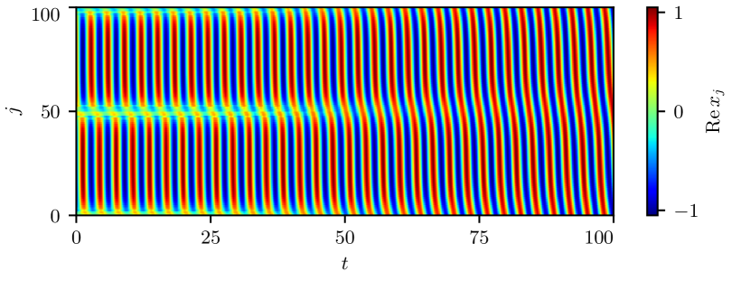
Figure 10: Real part $\operatorname{Re}x_{j}$ (indicated by color) of $100$ delay-coupled Stuart-Landau oscillators on a ring indexed by $j$ over time $t$. The coupling takes into account the ten nearest neighbors of an oscillator and acts with a constant time delay $\tau=\pi$ which is equivalent to the natural frequency $\omega=2$ of the oscillator. Initially the oscillators show a transient chimera state, i. e. a state in which a fraction of the oscillators is synchronized and another fraction is not synchronized. The chimera disappears with increasing time and the systems ends up in a state where all oscillators are synchronized with a phase-lag (chimera death). Figure replicated from [107, Fig. 3].

Transmission delays are common in physical networks, where they may impact synchronization processes of functionally similar constituting units [108]. Examples are optical systems [3] and gene expression networks [109]. In reaction-diffusion systems, such as the Gray-Scott model [110, 111], delays impact the occurrence of self-organized spatio-temporal patterns. For an overview of delay-coupled systems see [112]. The synchronization of networks with delay coupling has been addressed with a special focus on distributed delays [113], observing death and birth regions of amplitude synchronization [114]. Also, a general criterion for the synchronization of delay-coupled networks based on the networks topology has been derived [115].

In neural networks with time delay couplings [116], the synchronization of neurons may be studied with diffusive or with pulse-like delay couplings [117]. The delayed feedback of neural activity to the network has been shown to be able to suppress noise induced dynamics and thus to stabilize brain activity [118]. The type of delay, and its spatial distribution, have in general a pronounced influence on network activity [119].

From a more abstract perspective, the effect of time delay couplings on oscillatory systems has applications for control problems [120], as realizable in electric circuits [121]. Chimera states are observed in this kind of delay-coupled oscillatory networks [107, 122], that is states for which a finite fraction of the oscillators is synchronized, while the rest is fully desynchronized, i. e. chaotic (cf. Fig. 10). The interplay between the inherent dynamics of the network units and the delayed feedback can be used both to stabilize partially synchronized states [123], and to control the lifetime of chimeras [124]. In optical systems delay coupling can give rise to two-dimensional chimeras and soliton solutions [125].

Another application of delay coupling is the realization of reservoir computing networks [126], which are closely related to so-called echo state networks [127]. It has been shown that the time delayed feedback of a single optical unit allows information processing in a reservoir like manner [128, 4].

An externally driven system is considered consistent [129, 130, 131], if the system produces the same output, when presented with a certain input, independently of the initial internal state of the system. The concept of consistency is therefore an important feature for information processing networks. Further, the concept is closely related to synchronization of chaotic units in a network [131]. Consistency has been achieved with the help of time delay coupling for reservoir computing networks [132] and other optical networks [130, 131].

2.10 Long time delays

Time delays are considered long if they act on a substantially longer time scale than the internal dynamics. This is the case, e. g. for coupled optical systems, when the optical feedback via fiber transmission is slower than the dynamics of the lasers [133, 3]. Time delays may hence induce an additional time scale. In control theory [134, 135], long delays have a significant impact on stability regulation, with the consequence that the motion resulting from controlling the balance of an inverted pendulum differs qualitatively for short and long time delays [26].

Regarding the stability analysis of systems with long delays, an equivalence between the dynamics in the vicinity of a fixed point and a generalized reaction diffusion process has been worked out [136]. In the asymptotic limit, $\tau\to\infty$, the Lyapunov spectrum may be rescaled by $1/\tau$, in terms of the real part, with the resulting rescaled asymptotic spectrum being continuous [137, 138, 139]. The stability of fixed points and limit cycles becomes in this sense independent of the exact value of the delay in the long-delay limit [140, 141].

3 Characterizing the dynamics of time delay systems

We start with some preliminary remarks regarding the notation used for the subsequent discussion of a range of approaches and measures that identify and describe regular and chaotic dynamics in time delay systems.

3.1 Fixed points

Fixed point attractors often constitute the starting point when analyzing the dynamics of a time delay systems. The entire state history collapses, with (1) reducing to

$$F(x^{*},x^{*}) =0,\qquad\quad x^{*}=x(t)=x(t-\tau)\,.$$ (46)

Linear DDE, like (15), have the trivial fixed point $x^{*}=0$, the Mackey-Glass system (31) the fixed point $x^{*}=1$ (for $a=2b$ and $c>0$).

For a standard stability analysis [40] one considers a perturbation $\delta(t)$ to a given trajectory $x(t)$. For the DDE (1) one obtains

$$\frac{\mathrm{d}}{\mathrm{d}t}\Big{(}x(t)+\delta(t)\Big{)} =F\Big{(}x(t)+\delta(t),x(t-\tau)+\delta(t-\tau)\Big{)}\,,$$ (47)

which leads to Eq. (6) when expanding the flow $F$ into a first-order Taylor expansion around the fixed point solution $x(t)\equiv x^{*}$. Eq. (6) is itself a delay differential equation. For a further treatment the state history of the perturbation $\delta(t)$ needs to be known on a time interval $[t-\tau,t]$, which is however normally not the case.

In the vicinity of a fixed point $x^{*}$ one can however assume that the perturbation evolves exponentially, $\delta(t)=\delta(0)\,\e^{\Lambda t}$, as characterized by the complex local Lyapunov exponent $\Lambda$ (cf. Sect. 1.4). The time evolution (6) of the perturbation reduces then to

$$\dot{\delta}(t)=J_{\text{eff}}\,\delta(t)\,,\quad J_{\text{eff}}=J_{\text{o}}(x^{*},x^{*})+\e^{-\Lambda t}J_{\tau}(x^{*},x^{*})\,,$$ (48)

with an effective Jacobian $J_{\text{eff}}$ [39]. Applying (48) to the exponential ansatz for the perturbation, one obtains the characteristic equation

$$\Lambda=J_{\text{o}}+\e^{-\Lambda t}J_{\tau}\,,$$ (49)

which is a transcendental equation solved by infinitely many local Lyapunov exponents $\Lambda=\Lambda_{j}$. A special case of (49) is discussed in Sect. 1.5.

The perturbation $\delta(t)$ lives in the $N\to\infty$ dimensional phase space of states histories. The flow around a fixed point is governed therefore by the local Lyapunov exponents $\Lambda_{k}$,

$$x(t)=x^{*}+\delta(t),\quad\qquad\delta(t)=\sum\limits_{k=1}^{\infty}c_{k}\,\e^{\Lambda_{k}t}\,,$$ (50)

where $c_{k}$ and $\Lambda_{k}$ are complex (cf. Sect. 1.5.1). For real states $x=x(t)$, as assumed here, the local Lyapunov exponents come in complex conjugate pairs $\bar{\Lambda}_{k}=\Lambda_{k^{\prime}}$ whenever the imaginary part is non-zero.

Ordering the exponents $\Lambda_{k}$ with respect to the magnitude of the real part we have

$$\operatorname{Re}\Lambda_{1}\geq\operatorname{Re}\Lambda_{2}\geq\operatorname{Re}\Lambda_{3}\geq\ldots\,,$$ (51)

with the largest value $\operatorname{Re}\Lambda_{1}$ determining the stability of the fixed point. The steady state solution $x=x^{*}$ is stable for $\operatorname{Re}\Lambda_{1}<0$, and unstable otherwise.

3.2 Types of chaotic motion

Deterministic chaos [60, 142] can be classified along a series of distinct criteria, which are not necessarily mutually exclusive. This is in particular true for some recent classifications schemes discussed in this section, which describe in part different features of chaotic motion.

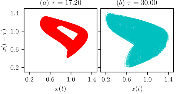
Figure 11: Trajectories of chaotic attractors in the Mackey-Glass system (31) in the stroboscopic projection $x(t)$-$x(t-\tau)$, for ($a$) $\tau=17.20$ and ($b$) $\tau=30.00$, both sampled over $t\in[0,5\cdot 10^{4}$].

3.2.1 Delay induced chaos

Stable fixed points and limit cycles existing in the limit $\tau\to 0$ are necessarily destabilized by a Hopf bifurcation when increasing $\tau$ continuously [40, 47]. The local Lyapunov exponents then first become complex. Once the time delay $\tau$ becomes large enough to be out of phase with the period $2\pi/\operatorname{Im}\Lambda_{1}$ of the oscillation, a perturbation $\delta(t)$ can increase in a self-reinforcing manner (cf. Fig. 2).

This mechanism is well documented for the Mackey-Glass system (31), for which a series of period doubling bifurcations leads to chaotic dynamics [59, 143]. The respective route to delay-induced chaos has been observed experimentally for a catalytic reaction [144]. We note, however, that the limit cycle appearing beyond the first Hopf bifurcation may remain stable [58], even tough it is non unexpected that chaos will eventually show up, given that DDEs are formally infinite dimensional.

In Fig. 11 we present the trajectories of two chaotic attractors of the Mackey-Glass system by a stroboscopic projection (cf. Sect. 3.6). We will show in the next Section that these two attractors differ qualitatively in terms their cross-correlation functions.

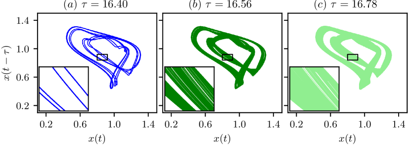
Figure 12: Stroboscopic projection of attractors of the Mackey-Glass system (31) for different values of the time delay $\tau$ and sampled over $t\in[0,5\cdot 10^{4}]$; insets magnifying the indicated area. ($a$) A limit cycle for $\tau=16.40$ with $8$ windings per period. ($b$) A partially predictable chaotic (PPC) attractor for $\tau=16.56$ with visible gaps in the fractal braid. ($c$) A partially predictable chaotic (PPC) attractor for $\tau=16.78$ with one extended fractal braid winding twice per period.

3.2.2 Partially predictable chaos

Chaotic attractors may fill a substantial part of the phase space, forming in this way a fractal structure (cf. Fig. 11). On the other hand, one can observe chaotic attractors differing in shape overall only slightly from a periodic orbit [145, 146, 147]. Such kind of attractors are also found for the Mackey-Glass system (31), as presented in Fig. 12 in comparison with a regular limit cycle. The insets magnifying the selected parts of the respective trajectories show that the chaotic attractors consist of a fractal braids with either a coarser structure, including gaps of all sizes, or fine fractal filaments.

The difference between the chaotic attractors shown in Figs. 11 and 12 can be quantified by the cross correlation

$$C(t) =\Big{\langle}\big{(}x_{\text{o}}(t)-\mu\big{)}\big{(}x_{1}(t)-\mu\big{)}\Big{\rangle}/\sigma^{2}$$ (52)

of a pair of trajectories $x_{\text{o}}(t)$ and $x_{1}(t)$ in the vicinity of an attractor with mean $\mu$ and variance $\sigma^{2}$. Included in (52) is an average over respectively initial conditions (for ordinary differential equations) and initial functions (for delay systems), as indicated by $\langle\cdot\rangle$. For delay systems one needs to average (52) in addition over a delay interval, viz to add an integral $\int_{t-\tau}^{t}\mathrm{d}t^{\prime}(\ldots)$, as in the definition (5) for the distance $d(t)$ between two state histories.

The cross-correlation is related via

$$1-C(t)=d^{2}(t)/(2\sigma^{2})$$ (53)

to the distance $d(t)$ between the two trajectories [30], where $d(t)$ is either the instantaneous distance (for ordinary differential equations), or the distance between state histories defined by Eq. (5).

A pair of trajectories is initially maximally correlated, in the sense that $C(t\!=\!0)\to 1$, when the initial distance of state histories $d(t\!=\!0)=\delta$ is small with respect to the extent $\sigma$ of the attractor, viz when $\delta\ll\sigma$. This is clearly true independently of the type of the attractor under consideration. Inter-trajectory correlations are retained in the long-term limit $t\to\infty$ for regular motion, that is, e. g., for fixed points and limit cycles, but fully lost for chaotic attractors [30]:

$$\lim\limits_{t\to\infty}C(t)\ =\ \left\{\begin{array}[]{cl}1&\text{regular motion}\\ 0&\text{chaotic attractor}\end{array}\right.\,.$$ (54)

The long-term limit is usually approximated by the Lyapunov prediction time $T_{\lambda}$ (cf. Sect. 3.4), which is inversely proportional to the maximal Lyapunov exponent (cf. Sect. 1.4), since $T_{\lambda}$ provides an estimate for the time needed for the exponential divergence of two trajectories to become sizable.

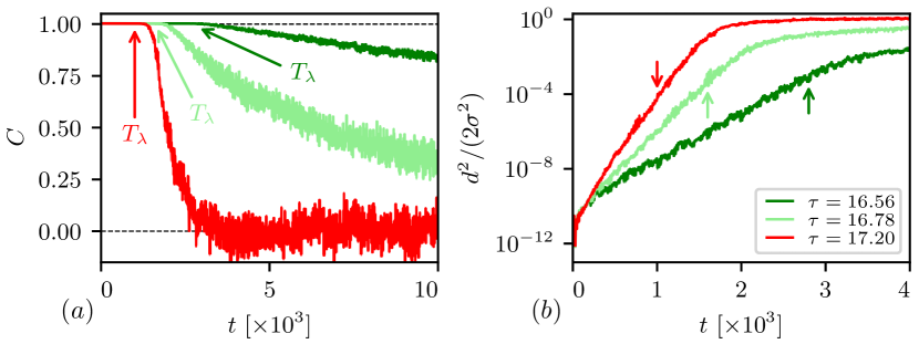
Figure 13: The cross-correlation $C$ of initially close ($\delta=10^{-6}$) pairs of trajectories for the chaotic attractors of the Mackey-Glass system shown in Figs. 11 and 12 (dark green: $\tau=16.56$, $T_{\lambda}=2791$; light green: $\tau=16.78$, $T_{\lambda}=1588$; red: $\tau=17.20$, $T_{\lambda}=1071$). An average over $100$ initial functions has been performed, with the arrows indicating the corresponding Lyapunov prediction times $T_{\lambda}$ (cf. Sect. 3.4). Shown is ($a$) the cross-correlation (52) over time and ($b$) a semi-log plot of the initial exponential divergence of the corresponding distance $d(t)$. Full decorrelation, which occurs strictly only in the long-term limit $C(t\!\to\!\infty)\to 0$, is sizable for classical chaos (red) for $t\approx T_{\lambda}$. The final decorrelation is much slower for partially predictable chaos (PPC, green).

In Fig. 13 the cross-correlation $C$ for the chaotic attractors from Figs. 11 and 12 is plotted over time, with the arrows indicating the respective Lyapunov prediction times $T_{\lambda}$. Also presented in Fig. 13 is the distance $d^{2}/(2\sigma^{2})$ in a semi-log plot that amplifies the initial exponential divergence of the two trajectories.

For some attractors the exponential initial decorrelation is followed by a second slower phase of linear decorrelation. The latter is due to diffusive motion of trajectories on the chaotic attractor along the braid tracing the formerly stable limit cycle [30].

• For the chaotic attractor with $\tau=17.20$ the exponential and diffusive loss of correlation happen on the same time scale, leading to an essentially fully uncorrelated motion when the Lyapunov prediction time $T_{\lambda}$ is reached. See Fig. 13. We term this type of behavior ‘classical chaos’.

• For $\tau=16.56$ and $\tau=16.78$ only the exponential initial decorrelation occurs within the Lyapunov prediction time, with the subsequent diffusive loss of correlation taking orders of magnitudes longer. This leads to a high residual correlation even after comparably long times $t\gg T_{\lambda}$, which implies that long-term coarse-grained predictions remain possible. This type of behavior has been denoted ‘partially predictable chaos’ (PPC) [30].

The distinction between classical and partially predictable chaos in terms of the cross-correlation function is

$$C(t\!\gg\!T_{\lambda})\quad\left\{\begin{array}[]{rl}=\!0&\text{classical chaos}\\ >\!0&\text{partially predictable chaos (PPC)}\end{array}\right.\,.$$ (57)

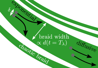
Figure 14: Sketch of the time-scale separation characterizing the divergence of trajectories for partially predictable chaos (PPC). Two initially close states $d(t\!=\!0)=\delta$ (gray bullets) diverge exponentially leading to an exponential drop of correlation (cf. Fig. 13). This process is limited by the width of the braid (green), such that by the Lyapunov prediction time $d(t\!=\!T_{\lambda})$ the distance is of the order of the braid width. The residual cross-correlation is lost subsequently due diffusive motion of trajectories along the fractal braid.

The time scale separation between exponential and diffusive decorrelation in PPC is closely related to the topology of the chaotic braids, as evident from the insets of Fig. 12. The initial exponential divergence occurring mainly perpendicular to a braid is limited by the braid width (cf. Fig. 14), which is therefore related to the distance $d(t\!=\!T_{\lambda})$ of two trajectories after the Lyapunov prediction time. Distinct fractal braids are on the other hand absent for classical chaos, with the consequence that the initial exponential decorrelation is not directly bounded by topology, see Figs. 11 and 13. Classical chaos and PPC are two limiting cases, with the distinction becoming somewhat fluid for very thick fractal braids.

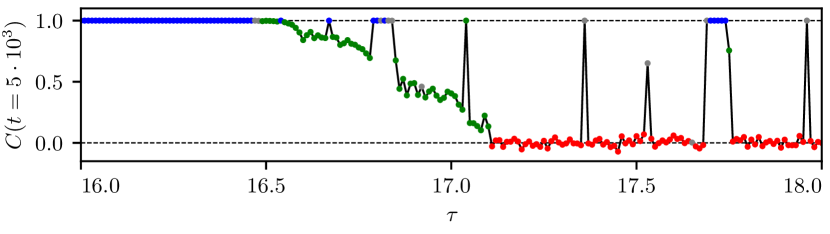
Figure 15: Long-term cross-correlation $C(t\!=\!5\!\cdot\!10^{3})$ of the Mackey-Glass system (31) as a function of the delay time $\tau$ and averaged over $100$ pairs of trajectories. The initial distance is $\delta=10^{-6}$. Regular motion (blue) is fully correlated $C=1$, with classical chaos being characterized by a complete loss of correlation $C\to 0$. Partially predictable chaos (PPC, green) occurs for chaotic motion with finite residual long-term correlation $1>C>0$.

PPC chaos is found for the Mackey-Glass system (31), e. g., close to the transition to chaos at a time delay $\tau\approx 16.48$. Figure 15 shows the residual correlation $C(t\!=\!5\cdot 10^{3})$, where $5\cdot 10^{3}\gg T_{\lambda}$, for pairs of trajectories and as a function of the time delay $\tau$ (cf. Sect. 3.4).

Note that the auto-correlation function [148, 149], which can be computed from a single trajectory, can be also used to describe the decorraltion process on chaotic attractors. However, it has been pointed out [30] that it is more challenging to quantify both the initial decorrelation and the linear loss of correlation in PPC through the auto-correlation function.

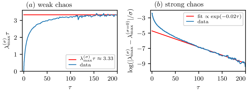
Figure 16: The maximal Lyapunov exponent $\lambda_{\text{max}}=\lambda_{\text{max}}^{(\sigma)}$ and the maximal instantaneous Lyapunov exponent $\lambda_{\text{max}}^{(\sigma=0)}$ of an attractor of the Lang-Kobayashi system [150] (cf. Eq. (58)). ($a$) The rescaled maximal Lyapunov exponent $\lambda_{\text{max}}^{(\sigma)}$ as a function of the time delay $\tau$ for weak chaos with coupling $\sigma=21\,\mathrm{ns}^{-1}$. In the limit of large delays $\tau\to\infty$ the maximal Lyapunov scales $\lambda_{\text{max}}^{(\sigma)}\sim 1/\tau$ inversely with the delay. ($b$) The logarithmic difference of the maximal $\lambda_{\text{max}}^{(\sigma)}$ and the instantaneous Lyapunov exponent $\lambda_{\text{max}}^{(\sigma=0)}$ over time delay $\tau$ for coupling $\sigma=12\,\mathrm{ns}^{-1}$. In the regime of strong chaos the difference vanishes exponentially in the limit $\tau\to\infty$ of large delays. Figure replicated from [151].

3.2.3 Weak and strong chaos

Several proposals for the distinction of weak and strong chaos, and thus for a differentiation between different types of chaotic motion, have been put forward [145, 152, 153]. For concreteness consider with

$$\dot{\mathbf{x}}(t) =\mathbf{F}_{1}\big{(}\mathbf{x}(t)\big{)}+\sigma\mathbf{F}_{2}\big{(}\mathbf{x}(t-\tau)\big{)}$$ (58)

a network of dynamical units $\mathbf{x}=(x_{1},\,x_{2},\,\dots)$ that are coupled instantaneously through $\mathbf{F}_{1}(\mathbf{x}(t))$, and delayed via $\mathbf{F}_{2}(\mathbf{x}(t-\tau))$ [151] (see also [34, 154]). The respective coupling strength is $\sigma$. Networks of this type are suitable for the description of chaos in coupled lasers [155, 3] and for the study of delay induced chaos (cf. Sect. 3.2.1),

A distinction between weak and strong chaos can now be made [151] for the special case that a fully synchronized state $\mathbf{s}(t)$, as defined by $x_{i}(t)\equiv s(t)$, is a solution of (58). The synchronized state may be stable or unstable. Stable synchronized states correspond to weak chaos, unstable synchronized states on the other side to strong chaos. One starts by defining two types of maximal Lyapunov exponents [151]:

• $\lambda_{\text{max}}^{(\sigma)}=\lambda_{\text{max}}$, which describes the divergence of trajectories from the synchronized state for the original system (58).

• $\lambda_{\text{max}}^{(\sigma\!=\!0)}$, which describes the divergence of trajectories from the synchronized state $\mathbf{s}(t)$ under the influence of only the instantaneous dynamics $\mathbf{F}_{1}(\mathbf{s}(t))$. Note, that $\mathbf{s}(t)$ is still a solution of the full system.

The distinction of weak and strong chaos follows then from the comparison of the full exponent $\lambda_{\text{max}}^{(\sigma)}$ and the instantaneous maximal Lyapunov exponent $\lambda_{\text{max}}^{(\sigma\!=\!0)}$:

• Weak chaos: For weak chaos the instantaneous Lyapunov exponent is negative, $\lambda_{\text{max}}^{(\sigma\!=\!0)}<0$, indicating that the evolution of perturbations at $\sigma=0$ is stable. The overall dynamics is at the same time unstable due to a positive full exponent, $\lambda_{\text{max}}^{(\sigma)}>0$. The synchronized state is then a stable but chaotic solution of (58).

• Strong chaos: For strong chaos both the instantaneous and the full maximal Lyapunov exponents are positive, $\lambda_{\text{max}}^{(\sigma\!=\!0)}>0$ and $\lambda_{\text{max}}^{(\sigma)}>0$. The system then settle into a global chaotic state, which is however not given by $\mathbf{s}(t)$.

Strong and weak chaos differ furthermore by their Lyapunov divergence times $T_{\lambda}\sim 1/\lambda_{\text{max}}$ (cf. Sect. 3.4), with the scaling $T_{\lambda}\sim\tau^{\eta}$ for large time delays $\tau\to\infty$, where $\eta=1$ for strong chaos and $\eta=0$ for weak chaos [151] (cf. Fig. 16).

According to this classification scheme, the Mackey-Glass system (31), which has a negative instantaneous Lyapunov exponent $\lambda_{\text{max}}^{(\sigma\!=\!0)}=b<0$, exhibits only weak chaos. Note that the coupling constant $a$ corresponds here to $\sigma$ and that bounded solutions need negative $b$. Vice versa, the difference between the attractors shown in Fig. 11 and Fig. 12 cannot be explained in terms of weak and strong chaos.

3.2.4 Intermittent and laminar chaos

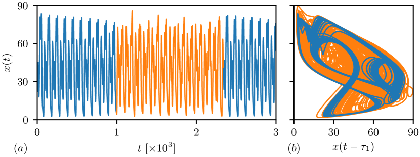
Figure 17: The solution $x(t)$ of a delayed feedback system with multiple time delays as defined by Eq. (59) for parameters $n=6$, $m=1$ and $\xi=38$, coupling strengths $k=0.2$ and $g=50$ and time delays $\tau_{1}=26$ and $\tau_{2}=26.25$. ($a$) A trajectory $x(t)$ showing intermittent chaos. The almost period dynamics (blue) is interseeded by chaotic bursts (orange). ($b$) Projection of the trajectory $x(t)$ shown in panel ($a$) with respect to the delayed state $x(t-\tau_{1})$. Highlighted (blue) is the braid of the quasi-periodic motion, which the solution follows most of the time. The chaotic bursts lead the system intermittently away from the braid. Figure replicated from [145].

Intermittent chaos is a type of chaos known from non-delayed systems [156, 157]. It is also observed in time delay systems [158, 159], e. g. in models describing gene regulation networks [145]. Consider the case that the delay term is with

$$\dot{x}(t) =-k\,x(t)+g\,f_{1}\big{(}x(t-\tau_{1})\big{)}\,f_{2}\big{(}x(t-\tau_{2})\big{)}$$ (59)

a product of a self-inhibitory and a self-activation term, $f_{1}$ and $f_{2}$, acting respectively with fixed but distinct delays $\tau_{1}$ and $\tau_{2}$. The coupling constants $k$ and $g$ determine the respective influence of the instantaneous and the delayed feedback on the dynamics.

Choosing Hill functions [160]

$$f_{1}(x)=1/\big{(}1+(x/\xi)^{n}\big{)}\,,\qquad f_{2}(x)=1-1/\big{(}1+(x/\xi)^{m}\big{)}$$ (60)

with parameters $n$, $m$ and $\xi$ for the activation and inhibition function [145], the solutions of (59) show intermittent chaos, which is in this case characterized by quasi-periodic dynamics interseeded by chaotic bursts. A typical trajectory is presented in Fig. 17.

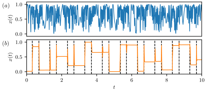
Figure 18: Chaotic solutions $x(t)$ of (61), as a function of time $t$, for $A=0.9/(2\pi)$ and $T=200$. The corresponding Lyapunov exponents are shown in Fig. 8. ($a$) Turbulent chaos for a conservative delay with $\tau_{\text{o}}=1.54$. ($b$) Laminar chaos for dissipative delay with $\tau_{\text{o}}=1.51$. The solution jumps between different laminar levels, where the height $h_{n}$ of the levels and the switching times $T_{n}$ (indicated by vertical dashed lines) can be predicted by an appropriate mapping. Figure replicated from [31].

Laminar chaos is on the other side closely related to the concept of dissipative time-varying delay [32] (cf. Sect. 2.5). An example of a system with time-varying feedback for which laminar chaos is observed is [31]

$$\frac{1}{T}\dot{x}(t) =-x(t)+4x\big{(}R(t)\big{)}\Big{(}1-x\big{(}R(t)\big{)}\Big{)},\quad\quad R(t)=t-\tau_{\text{o}}-A\sin(2\pi t)\,,$$ (61)

where $T$ is the overall time-scale. The access function $R(t)$, which enters (61) via a logistic feedback coupling, incorporates here a superposition of a constant delay $\tau_{\text{o}}$ and a sinusoidal contribution of amplitude $A$. Depending on the parameters, the dynamics may jump between constant plateaus of laminar motion, as illustrated in Fig. 18. The system is chaotic because both the sequence of plateau heights and the sequence of plateau durations exhibit non-regular dynamics [31]. For comparison a case of classically turbulent chaotic dynamics is shown as well.

Laminar chaos is not to be confused with intermittent chaos: for the first the laminar plateaus have a chaotically distributed height, while for the latter the chaotic bursts are framed by laminar or quasi-periodic oscillations of similar amplitudes.

3.2.5 Transient chaos

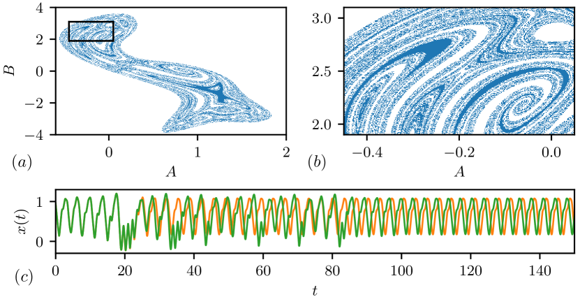
Figure 19: ($a$) Basin of attraction of the delayed logistic Eq. (63) for $\tau=1$ and $\beta=6.16$, with $A$ being the offset and $B$ the frequency of the initial function (62) on a $2^{11}\times 2^{11}$ grid. Parameter pairs $(A,B)$ marked blue correspond to an initial function for which the system (63) converges to a periodic attractor. Else the motion diverges as $\lim_{t\to\infty}x(t)=-\infty$. ($b$) Magnifying the parameter region marked by the black square in panel ($a$) reveals the fractal character of the basin of attraction. Its fractal dimension is found to be $D_{\text{f}}=1.85\pm 0.01$ (cf. Sect. 3.8.3). ($c$) Two solutions of DDE (63) for $\tau=1$ and $\beta=6.16$, starting at initial functions (62), with parameters $B_{1}=-0.95$ and $A_{1}=0.947$ and respectively with $B_{2}=B_{1}$ and $A_{2}=A_{1}+10^{-4}$. The trajectories experience transient chaos before joining the same periodic attractor, albeit with a phase shift. Figure replicated from [161].

The chaotic attractors discussed in Sects. 3.2.1 to 3.2.4 are asymptotically stable, i. e. the dynamics settles onto the attracting set in the long-term limit $t\to\infty$. However, it is known that (asymptotically) unstable, fractal sets in the phase space of a system, so-called chaotic saddles [162, 163], can cause initially close-by trajectories to decorrelate. The motion of a trajectory in the vicinity of a chaotic saddle is termed transient chaos [164, 165, 166]. Transiently chaotic motion is furthermore accompanied by fractal basin boundaries in the phase space of the system. In the case of a time delay system this is reflected as a fine-grained subdivision of the space of initial functions. Small changes of the initial condition may then lead to different asymptotic attractors.

For DDE a trajectory is uniquely determined by an initial function (2), as defined on an initial time interval. A practical way to scan the space of possible initial functions is to sub-sample using functions parameterized by a finite number of parameters [161, 14]. An arbitrary but suitable choice is

$$\varphi(t)=A+\sin(Bt)\qquad\text{ for }t\in[-\tau,0]\,,$$ (62)

where the initial function $\varphi(t)$ is parameterized by an offset $A$ and a sinusoidal with frequency $B$. Using (62) for the delayed logistic equation

$$\dot{x}(t)=-x(t)+\beta x(t-\tau)\big{(}1-x(t-\tau)\big{)}$$ (63)

with a fixed time delay $\tau=1$ and a coupling strength $\beta=6.16$ one finds that for almost any pairs $(A,B)$ of parameters entering $\varphi(t)$ via (62) the motion is not bound, that is $\lim_{t\to\infty}x(t)=-\infty$. Only for certain combinations of parameters from a fractal set in the parameter set shown in Fig. 19 the motion settles to a periodic attractor in the long term. As argued in [161], the presence of a chaotic saddle induces transient chaos (cf. Fig. 19).

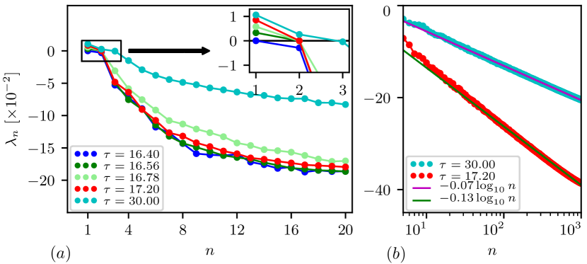
Figure 20: The largest global Lyapunov exponents $\lambda_{n}$ of the Mackey-Glass system (31), as computed with Benettin’s method and for different delays $\tau$ (cf. Sect. 4.2.2). ($a$) As in Figs. 11 and 12, for regular motion ($\tau=16.40$, blue), for PPC ($\tau=16,56$, green; $\tau=16.78$, light green) and classical chaos ($\tau=17.20$, red). The hyper-chaotic attractor ($\tau=30.00$, cyan) has two positive exponents. ($b$) A semi-log plot of the extended spectrum for the chaotic attractors shown in Fig. 11. The fits indicate logarithmic scaling $\lambda_{n}\sim-\log n$ in the limit $n\to\infty$, where $n$ is the index.

Table 1: Scheme for identifying different types of dynamics using the number of positive and zero global Lyapunov exponents $\lambda_{\text{max}}=\lambda_{1}\geq\lambda_{2}\geq\ldots\,$ [46].

	Lyapunov exponents
dynamics	positive	zero	largest neg.
stable fixed point			$\lambda_{\text{max}}<0$
limit cycle		$\lambda_{\text{max}}=0$	$\lambda_{2\phantom{+1}}<0$
hypertorus ($d$ dim.)		$\lambda_{\text{max}},\ldots,\lambda_{d}=0$	$\lambda_{d+1}<0$
chaos	$\lambda_{\text{max}}>0$	$\lambda_{2\phantom{+1}}=0$	$\lambda_{3\phantom{+1}}<0$
hyperchaos	$\lambda_{\text{max}},\ldots,\lambda_{k}>0$	$\lambda_{k+1}=0$	$\lambda_{k+2}<0$

3.3 Lyapunov spectrum

Chaotic attractors are considered to be strange in the sense that they are overall contracting [38, 42], being characterized on the other hand by at least one positive global Lyapunov exponent, as defined in Sect. 1.4.

As an illustration we present in Fig. 20 the spectrum of global Lyapunov exponents of the Mackey-Glass system (31) for different values of the time delay $\tau$. The largest Lyapunov exponent vanishes for regular motion (limit cycles), for which an initial deviation $\delta$ does not grow nor vanish on the average. This is consistent with the definition of the maximal Lyapunov as an average over the attractor. The spectrum of Lyapunov exponents is in contrast very broad on short time scales [30].

For chaotic motion at least one exponent is positive, $\lambda_{\text{max}}>0$, with chaotic motions with two or more positive exponents being termed hyperchaotic [167, 46]. This is the case in Fig. 20 for $\tau=30.00$. Note that all strange attractors have in addition one vanishing exponent describing the neutral flow along the trajectory. A categorization of the chaotic dynamics derived from the spectrum of Lyapunov exponents is given in Table 1.

It can be shown analytically [47], that the Lyapunov spectrum of a DDE with linear dependence on the instantaneous state $x(t)$ and a single constant time delay scales logarithmically, $\lambda_{n}\sim-\log n$, as a function of the index $n$, when $n\to\infty$. This results holds for the two Lyapunov spectra of the Mackey-Glass system shown in Fig. 20. The scaling is in contrast linear for DDE with time-varying $\tau=\tau(t)$ that are dissipative [32], as discussed in Sect. 2.3.

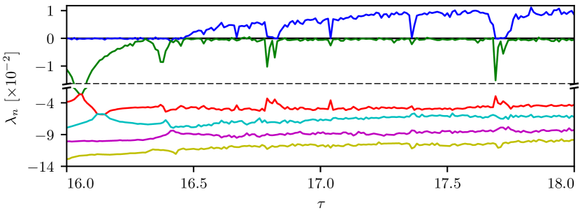
Figure 21: As a function of the delay $\tau$, the six largest Lyapunov exponents $\lambda_{n}$ of the Mackey-Glass system (31). Note the change in the scaling of the vertical axis indicated by the dashed horizontal line.

3.4 Lyapunov prediction time

For the Mackey-Glass system (31), the evolution of the six largest global Lyapunov exponents as a function of the time delay is presented in Fig. 21. The maximal exponent $\lambda_{\text{max}}$ changes from zero to a positive value at $\tau\approx 16.45$, the classical indicator of the transition from regular motion to chaos.

The maximal Lyapunov exponent $\lambda_{\text{max}}$ describes by definition the maximum rate of divergence, or the minimum rate of convergence (for positive and respectively for negative exponents). With the distance of two trajectories scaling as $\sim\delta\exp(\lambda_{\text{max}}t)$, one defines the Lyapunov prediction time $T_{\lambda}$ as

$$T_{\lambda}(\delta,d_{\text{p}}) =\frac{1}{\lambda_{\text{max}}}\log\left(\frac{d_{\text{p}}}{\delta}\right)\,.$$ (64)

It quantifies the time it takes the exponential divergence of two trajectories with initial distance $\delta$ to reach a final distance $d_{\text{p}}$ (cf. Fig. 1). The exact values for $d_{\text{p}}$ and $\delta$ are not critical, due to the logarithmic discounting in (64).

In Table 2 the four largest Lyapunov exponents for the attractors of the Mackey-Glass system shown in Figs. 11 and 12 are listed together with the corresponding Lyapunov prediction times $T_{\lambda}$. One finds that the thin chaotic braids of PPC also lead to longer predictability in the regime of exponential divergence (cf. Sect. 3.2.2).

Table 2: The largest four Lyapunov exponents and the Lyapunov prediction time $T_{\lambda}$, as defined by (64), for the attractors of the Mackey-Glass system (31) shown in Figs. 11 and 12. The parameters entering (64) are $d_{\text{p}}=10^{-2}$ and $\delta=10^{-6}$. For orientation the zero Lyapunov exponent is printed in bold.

$\tau$		$16.40$	$16.56$	$16.78$	$17.20$	$30.00$
dynamics		regular	PPC	PPC	chaos	hyperchaos
$T_{\lambda}$		-	$2791$	$1588$	$1071$	$\phantom{0}867$
$\lambda_{\text{max}}$	[$\times 10^{-2}$]	$\phantom{-}\mathbf{0.0}$	$\phantom{-}0.3$	$\phantom{-}0.6$	$\phantom{-}0.9$	$\phantom{-}1.1$
$\lambda_{2}$	[$\times 10^{-2}$]	$-0.3$	$\phantom{-}\mathbf{0.0}$	$\phantom{-}\mathbf{0.0}$	$\phantom{-}\mathbf{0.0}$	$\phantom{-}0.3$
$\lambda_{3}$	[$\times 10^{-2}$]	$-5.3$	$-5.0$	$-5.3$	$-4.8$	$\phantom{-}\mathbf{0.0}$
$\lambda_{4}$	[$\times 10^{-2}$]	$-7.2$	$-7.4$	$-6.7$	$-6.4$	$-1.5$

3.5 Phase space contraction rate

The phase space contraction rate $\kappa$ is an effective tool to quantify the behavior of the flow in finite dimensional continuous-time systems [40]. It describes the evolution of a volume element $V$ in the phase space over time

$$V(t) =V_{\text{o}}\;\e^{\kappa t}\,,$$ (65)

where the initial volume is denoted $V_{\text{o}}$ [168]. The sign of the phase space contraction rate indicates whether a system is dissipative, $\kappa<0$, conservative, $\kappa=0$, or whether energy is taken up when $\kappa>0$. The contraction rate is a local quantity that may vary strongly within phase space. For stable limit cycles and chaotic attractors the contraction rate needs to be negative when averaged over the attracting set, but not locally [169].

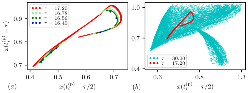
Figure 22: Poincaré sections (defined by $x_{\text{p}}=0.85$ in Eq. (68)) for the Mackey-Glass system (31), sampled over time $t\in[0,10^{4}]$ and projected to states $x(t-\tau/2)$ and $x(t-\tau)$, at the intersection times $t\to t_{i}^{(p)}$. ($a$) The periodic trajectory ($\tau=16.40$, blue) crosses the Poincaré plane eight times, whereas one observes extended fractal sets for PPC ($\tau=16.56$, green; $\tau=16.78$, light-green). For classical chaos ($\tau=17.20$, red) the fractal set has a larger extent than for PPC. ($b$) The Poincaré sections of classical chaos ($\tau=17.20$, red), as in ($a$), and for hyperchaos ($\tau=30.00$, cyan). Compare Figs. 11 and 12 and Table 2.

For a finite dimensional system the contraction rate is given by the sum of local Lyapunov exponents, viz as $\kappa=\sum_{n}\Lambda_{n}$. The situation is less clear for infinite dimensional time delay systems, for which the number of negative Lyapunov exponents diverges [47], as discussed in Sect. 1.4, as $\Lambda_{n}\to-\log n$ for $n\to\infty$. In the phase space of state histories the contraction rate is therefore formally diverging,

$$\kappa =\lim\limits_{N\to\infty}\sum\limits_{n=1}^{N}\Lambda_{n}\ =\ -\infty\,,$$ (66)

and hence not well defined for time delay systems.

3.6 Poincaré section

A widely used tool for the analysis of the flow in reduced dimensions is the Poincaré section [170, 40]. For a dynamical system with dimension $N$ the Poincaré hyperplane $P$ has dimension $N-1$, which is still infinite for a DDE, for which the phase space is given by the formally infinite-dimensional space of state histories $\mathbf{X}(t)=\{x(t^{\prime})\}$, where $t^{\prime}\in[t-\tau,t]$ (cf. Sect. 1.3). The intersections of a trajectory $\mathbf{X}(t)$ in the space of state histories with the selected hyperplane $P$ defines via

$$\mathbf{X}^{(\text{p})}_{i}\equiv\mathbf{X}(t^{(\text{p})}_{i}),\qquad\quad\mathbf{X}(t^{(\text{p})}_{i})\in P,\qquad\quad\mathbf{X}^{(\text{p})}_{i}\to\mathbf{X}^{(\text{p})}_{i+1}\,,$$ (67)

a map $\mathbf{X}^{(\text{p})}_{i}\to\mathbf{X}^{(\text{p})}_{i+1}$ between consecutive crossings. A convenient way to define the intersections, and the respective crossing times $t^{(\text{p})}_{i}$, is to choose a value $x_{\text{p}}$, such that

$$x^{(\text{p})}_{i}\equiv x(t^{(\text{p})}_{i})=x_{\text{p}}$$ (68)

holds for the trajectory $x(t)$ in configuration space.

The map between consecutive intersections, also called first recurrence map, defined by the Poincaré section can be studied also in configuration space, $x^{(\text{p})}_{i}\to x^{(\text{p})}_{i+1}$. Apart from the location, one may also consider the direction of the intersection and restrict, as it is usually done, the Poincaré map to consecutive intersections characterized by the same direction.

For graphical illustrations in two dimensions it is custom to select two states from the state histories that are separated in time, such as $x(t-\tau_{1})$ and $x(t-\tau_{2})$, as representatives of the state histories defined by the intersection of the trajectory with the Poincaré hyperplane. For a system with a fixed time delay $\tau$, a convenient choice for the Poincaré section is $\tau_{1}<\tau_{2}=\tau$.

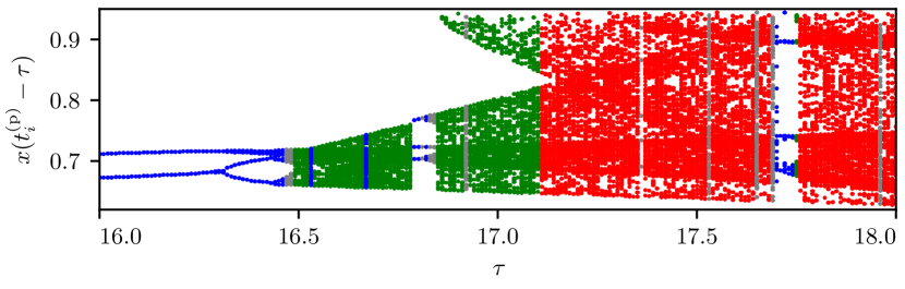
Figure 23: Poincaré sections of the Mackey-Glass system (31) for a range of time delays $\tau$, as projected to $x(t^{(\text{p})}_{i}-\tau)$ (for details see Fig. 22). The transition from periodic motion (blue) to PPC (green) occurs due to a period-doubling cascade. PPC is distinguished from classical chaos (red) by its finite residual correlation (cf. Fig. 15).

In Fig. 22 the Poincaré section for the attractors of the Mackey-Glass system (31) shown in Figs. 11 and 12 are compared. Note that periodic motion, which corresponds to fixed points of the Poincaré map, may also be of higher period, like $x^{(\text{p})}_{1}\to\ldots\to x^{(\text{p})}_{8}\to x^{(\text{p})}_{1}$. Partially predictable and classical chaotic attractors form on the other hand extended sets resembling thin filaments in the projection of the Poincaré hyperplane, which can be shown to be self-similar [38, 171]. Moreover, one observes that hyperchaotic attractors tend to be more space filling in terms of the Poincaré section (cf. Sect. 3.8).

In Fig. 23 a color-coded bifurcation diagram of the Mackey-Glass system generated using a one dimensional projection of the Poincaré section is presented. The cascade of period-doubling bifurcations [172, 173] (also called Brunovsky bifurcation [174]) leading to partially predictable chaos (PPC) upon increasing the time delay $\tau$ is evident, with the phase of PPC being interseeded by periodic windows. The transition from PPC to classical chaos then induces a fast drop in correlations, as detailed out in Sect. 3.2.2.

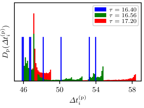
Figure 24: For different attractors of the Mackey-Glass system (31), the distribution $D_{\text{p}}$ (in arbitrary units) of the time intervals $\varDelta t^{(\text{p})}_{i}$ between consecutive Poincaré sections (cf. Fig. 22). $120$ bins have been used. The periodic attractor ($\tau=16.40$, blue) cuts the Poincaré plane eight times (cf. Fig. 22) leading to a distribution that consists of peaks of equal height. For partially predictable (PPC, $\tau=16.56$, green) and classical chaos ($\tau=17.20$, red) the distribution widens around the peaks.

Another aspect of the Poincaré map involves the time intervals between consecutive sections, the recurrence time [175, 176]:

$$\varDelta t^{(\text{p})}_{i} =t^{(\text{p})}_{i+1}-t^{(\text{p})}_{i}\,.$$ (69)

The distribution of the recurrence times of three attractors is presented in Fig. 24. As the regular motion crosses the Poincaré plane periodically, the inter-section times are discrete peaks of equal probability.

For partially predictable chaos the distribution is blurred, with some residual resemblance to the original periodic peaks. As the topology of the classical chaotic state deviates from periodic and PPC attractors, the distribution becomes more wide-spread.

3.7 The power spectrum of attractors

In addition to the distribution of return times in the Poincaré plane, the power spectrum $S(\omega)$ (the spectral density) of an attractor can be used to characterize classes of distinct time delay dynamics [177, 178]. It is evaluated from the Fourier transformation $\hat{x}(\omega)$ of a trajectory $x(t)$ as

$$\hat{x}(\omega)=\int\limits_{-\infty}^{\infty}\!\!\!\mathrm{d}t\;x(t)\;\e^{-\imath\omega t}\,,\quad\qquad S(\omega)=\lVert\hat{x}(\omega)\rVert^{2}\,,$$ (70)

which is in practice evaluated using numerical tools, such as the Fast Fourier Transformation [179, 180]. For comparison, Fig. 25 shows the power spectra of a periodic, a partially predictable and a classical chaotic attractor of the Mackey-Glass system (31).

The frequency has been rescaled in Fig. 25 by the frequency $\omega_{\text{p}}=0.016$ of the periodic trajectory, which corresponds to the period $T_{\text{p}}=2\pi/\omega_{\text{p}}\approx 390$. As a consequence of the eightfold winding of the limit cycle the main peak in the corresponding power spectrum occurs at $\omega_{\text{qp}}=8\,\omega_{\text{p}}$, with a winding time of $T_{\text{qp}}=T_{\text{p}}/8\approx 48.8$ (cf. Fig. 12 and Sect. 3.6). The remainder of the spectrum of the limit cycle consists of sharp peaks at integer multiples of the frequency $\omega_{\text{p}}$.

The peaks in the spectral density of the PPC attractor shown in Fig. 25 overlap with the spectrum of the periodic attractor, having in addition smaller contributions close to the main peak. This behavior results from the fact that the topology of the partially predictable chaotic attractor resembles the topology of the former limit cycle (cf. Fig. 12). For the frequency spectrum of the classical chaotic attractor one can also observe major contributions close to the frequencies of the periodic orbit, this time however with a substantial spread [181, 178].

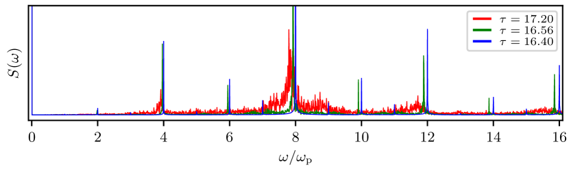
Figure 25: The spectral density $S(\omega)$ (in arbitrary units) as a function of the frequency $\omega$, of different attractors of the Mackey-Glass system (31). The data was obtained by sampling trajectories over $t\in[0,5\cdot 10^{4}]$, with a resolution of $\varDelta t=10^{-1}$. The frequency is normalized by the frequency $\omega_{\text{p}}\approx 0.016$ of the periodic attractor found for $\tau=16.40$. For periodic motion ($\tau=16.40$, blue) the distribution consists of isolated peaks, which widen when going from PPC ($\tau=16.56$, green) to classical chaos ($\tau=17.20$, red).

Table 3: Comparing the Mori dimension $D_{\text{M}}$ and the Kaplan-Yorke dimension $D_{\text{KY}}$ to the fractal dimension $D_{\text{f}}$ and the correlation dimension $D_{\text{c}}$ of the attractors shown in Figs. (11) and (12). PPC stands for partially predictable chaos.

$\tau$	$D_{\text{M}}$	$D_{\text{KY}}$	$D_{\text{f}}$	$D_{\text{c}}$	dynamics
$16.40$	$1$	$1.094$	$1.008\pm 0.014$	$1.000\pm 0.001$	regular
$16.56$	$2$	$2.061$	$1.968\pm 0.005$	$1.964\pm 0.003$	PPC
$16.78$	$2$	$2.110$	$2.040\pm 0.007$	$2.070\pm 0.005$	PPC
$17.20$	$2$	$2.180$	$2.133\pm 0.009$	$2.146\pm 0.003$	classical chaos
$30.00$	$3$	$3.707$	$3.258\pm 0.026$	$3.197\pm 0.022$	hyperchaos

3.8 The dimension of attractors

An interesting point when investigating chaotic dynamics is the dimension of the attracting set of points in phase space. Different measures describing the number of independent dimensions needed for embedding the attractor, based either on the geometric properties [171], on the change of the entropy [182], and on the correlation of trajectories on the attractor [183], have been proposed in this context. The embedding dimension is of particular relevance for infinite dimensional systems, such as a DDE, as it determines the number of time delays $\tau_{i}\in[0,\tau]$ needed to span a minimal Poincaré hypercube $\{x(t-\tau_{i})\}$. An attractor can then be studied without information loss via its projection onto the minimal Poincaré hypercube.

In this section several different definitions for the dimension of an attractor are reviewed, of which two are computed from the Lyapunov spectrum (cf. Sect. 1.4), with the remaining two definitions retrieving geometric information from Poincaré sections. An overview of the respective estimates for the attractors shown in Figs. (11) and (12) is given in Table 3, as discussed below.

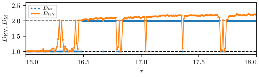
Figure 26: The Mori dimension $D_{\text{M}}$ and the Kaplan-Yorke dimension $D_{\text{KY}}$, defined respectively by (71) and (72), for the Mackey-Glass system (31). The estimates have been computed from the Lyapunov spectrum as a function of the time delay $\tau$ (cf. Fig. 21). For time delay systems the Mori dimension $D_{\text{M}}$ attains only integer values, which is the number of dimensions for embedding the Poincaré section of the corresponding attractor. The Kaplan-Yorke dimension $D_{\text{KY}}\geq D_{\text{M}}$ is in contrast able to probe the fractal character of the attractors.

3.8.1 Mori dimension

The Mori dimension $D_{\text{M}}$ is calculated from the ordered spectrum of global Lyapunov exponents $\lambda_{n}$ via [47, 168]

$$D_{\text{M}} =p+\frac{\sum_{\lambda_{n}>0}\,\lambda_{n}}{\sum_{\lambda_{n}<0}\,\lvert\lambda_{n}\rvert}\,,\qquad\quad\lambda_{\text{max}}=\lambda_{1}\geq\lambda_{2}\geq\ldots$$ (71)

where $p$ denotes the number of non-negative Lyapunov exponents $\lambda_{n}\geq 0$. It is constructed to weigh the contribution of expanding dimensions $\lambda_{n}>0$ with respect to the contribution of contracting dimensions $\lambda_{n}<0$.

For time delay systems the Mori dimension reduces to $D_{\text{M}}=p$, due to the fact that the spectrum of negative exponents is not integrable, viz that $\lambda_{n}\sim-\log n$ for $n\to\infty$ (cf. Sect. 1.4). The results for the Mori dimension of the Mackey-Glass system (31) are given in Fig. 26 as function of the time delay $\tau$, see also Fig. 21. The Mori dimension is $D_{\text{M}}=1$ for limit cycles and $D_{\text{M}}=2$ for both classical and partially predictable chaos, increasing further for hyperchaos. A comparison is presented in Table 3.

3.8.2 Kaplan-Yorke dimension

The Kaplan-Yorke dimension [47, 184], originally also called Lyapunov dimension [185], is defined by

$$D_{\text{KY}} =j+\frac{\sum_{n=1}^{j}\lambda_{n}}{\lvert\lambda_{j+1}\rvert}\,,$$ (72)

which resembles the definition of the Mori dimension (71). Here $j$ is the largest index for which the sum of Lyapunov exponents is not negative:

$$\sum\limits_{n=1}^{j}\lambda_{n}\geq 0\qquad\text{and}\qquad\sum\limits_{n=1}^{j}\lambda_{n}+\lambda_{j+1}<0\,.$$ (73)

The first sum in (73) takes into account the $j$ largest dimensions describing the overall expansion of the system, that is the maximal number of exponents for which the phase volume expansion, as defined in Sect. 3.5, is still positive.

With the second term in (72) the non-integer part of the fractal dimension of a chaotic attractor is estimated as the ratio of the phase volume expansion generated by the $j$ largest exponents, $\sum_{i=1}^{j}\lambda_{n}$, and the magnitude of the contraction rate due to the next largest exponent, $\lambda_{j+1}$. From the second condition in (73) one infers that $j\leq D_{\text{KY}}<j+1$.

The Kaplan-Yorke dimension is used to characterize attractors in instantaneous and delayed systems [186], e. g., when modelling turning processes [187].

With $p$ being the number of non-negative Lyapunov exponents, it follows that $p\leq j$ and consequently that the Mori dimension is a lower bound for the Kaplan-Yorke dimension, $D_{\text{M}}\leq D_{\text{KY}}$. This relation shows up in Fig. 26, where both estimates are presented in comparison. The Mori and the Kaplan-Yorke dimension take the same value $D_{\text{M}}=D_{\text{KY}}=1$ when the underlying motion is periodic (limit cycle). For chaos the Kaplan-Yorke dimension is fractal and hence larger, $D_{\text{KY}}>D_{\text{M}}$. See also Fig. 21. The Kaplan-Yorke dimension does however not distinguish qualitatively between classical and partially predictable chaos (cf. Table 3 and Fig. 15).

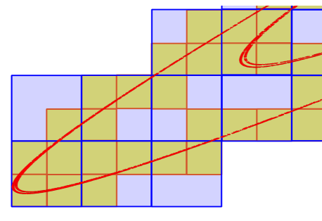
Figure 27: Sketch of the box-counting method for computing the fractal dimension $D_{\text{f}}$ of a trajectory (red lines), as projected to a two-dimensional plane (cf. Fig. 22), by counting the number of boxes $N(\epsilon)$ (orange squares) it takes to cover the attracting set in relation to the box size $\epsilon$.

3.8.3 Fractal dimension

The fractal dimension $D_{\text{f}}$ measures the space-filling capacity of a geometric set [188], or of a set of points embedded in a $D\geq D_{\text{f}}$ dimensional space [171], e. g. such as a time series $\left\{\mathbf{x}_{i}=x(t_{i})\right\}$ sampled equidistant in time from a trajectory $x(t)$. It is effectively defined by the scaling exponent of the number $N(\epsilon)$ of $D$ dimensional boxes with box size $\epsilon$ needed to cover the set in the limit of small boxes:

$$N(\epsilon) \sim\epsilon^{-D_{\text{f}}}\qquad\text{for}\qquad\epsilon\to 0\,.$$ (74)

Equivalently one has

$$D_{\text{f}} =-\lim\limits_{\epsilon\to 0}\frac{\log N(\epsilon)}{\log\epsilon}\,.$$ (75)

The method, which is also called box-counting, is illustrated in Fig. 27 for the two-dimensional projection of an attracting set. For a simple geometric object the fractal dimension is integer, as it corresponds to the number of linearly independent vectors needed to span the object. However, for objects with a more complicated, e. g. fractal structure, such as the Poincaré section of chaotic attractors, the fractal dimension attains non-integer values. It has been conjectured that the fractal and the Kaplan-Yorke dimension may coincide [185].

In order to determine the fractal dimension of an attractor one usually considers two options: either retrieving the fractal dimension from a trajectory on the attractor; alternatively one performs the box-counting on the Poincaré section of the trajectory and determines the fractal dimension of the sections, which neglects by definition of the section one dimension. With the Poincaré hyperplane of a DDE being infinite-dimensional, one then works with a projection, with the dimension $D$ of the projection being large enough to embed the attractor in question, that is at least the overall embedding dimension minus one.

There are different approaches for embedding an infinite-dimensional attractor in a time delay system to a space spanned by $D<\infty$ dimensions. The so-called time delay embedding or Takens’ embedding is one of the most widely used techniques [189, 190]. In practice one selects $D$ time delays $\tau_{1},\tau_{2},\ldots,\tau_{D}$ for the embedding, such that $\mathbf{x}_{i}=(x(t_{i}-\tau_{1}),x(t_{i}-\tau_{2}),\ldots,x(t_{i}-\tau_{D}))$ corresponds to the projection of the time series sampling the attractor. A convenient choice for the embedding delays is $\tau=\tau_{1}>\tau_{2}>\ldots>\tau_{D}>0$, where $\tau>0$ denotes the delay of the system. Note that Takens embedding does not require the underlying dynamics to be delayed. It rather samples past states in order to describe a system’s state. How to find the minimal embedding dimension, i. e. how to determine the smallest possible $D$ for which the embedded attractor has the same features as the original dynamics, is a problem that has been studied extensively [191, 192].

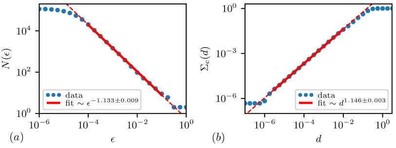
Figure 28: ($a$) Number of boxes $N(\epsilon)$ over the box size $\epsilon$ (blue bullets) for the Poincaré section of the chaotic attractor $\tau=17.20$ embeded into two dimensions as presented in Fig. 22 on log-log axes. The slope of the fit (red line) yields the estimate $D_{\text{f}}=1+1.133\pm 0.009$ for the fractal dimension $D_{\text{f}}$ of the attractor. ($b$) The correlation integral $\Sigma_{\text{c}}(d)$, as defined by Eq. (76), as a function of the distance $d$ (blue bullets) for the chaotic attractor $\tau=17.20$ shown in Fig. 22, on log-log axes. The slope of the fit (red line) yields an estimate $D_{\text{c}}=1+1.146\pm 0.003$ for the correlation dimension of the attractor.

For the box counting of the chaotic attractor in the Mackey-Glass system we use the time series of the states obtained from the Poincaré section in Fig. 22, i. e. $\mathbf{x}_{i}=(x(t^{(\text{p})}_{i}-\tau_{1}),\ldots,x(t^{(\text{p})}_{i}-\tau_{D}))$. The result is plotted in Fig. 28, with both the number of boxes $N(\epsilon)$ and the box size $\epsilon$ being logarithmic. From a linear fit one retrieves the exponent of the fractal dimension of the Poincaré section, which is here $D_{\text{f}}^{(2)}\approx 1.13$. The fractal dimension of the attractor, which is shown in Fig. 11, is in consequence $D_{\text{f}}\approx 2.13$. The range of box sizes for which the linear fit holds is $\epsilon>10^{-4}$, due to the circumstance that the number of points in the Poincaré section is limited to $\sim\!10^{5}$, for computational reasons.

A comparison of the estimates for the fractal and the Kaplan-Yorke dimension is given in Table 3. For regular motion and classical chaos the results are in good agreement, though for PPC a substantial quantitative discrepancy is observed. We note that the dimension used for embedding the Poincaré section has been selected to be the Mori dimension. The fractal dimension would however change only for an embedding with of insufficient dimension.

Table 4: Comparing the exponent $K$ from the Gottwald-Melbourne $0-1$ test and the distance scaling exponent $\nu$ of the Mackey-Glass system (31) for different delays $\tau$. $K$ is computed from $5\cdot 10^{3}$ points sampled with step size $\varDelta t=10$ and $\zeta=2$ in (81) (cf. Fig. 31). The distance scaling exponent $\nu$ is averaged over $100$ pairs trajectories starting from initial distance $\delta=10^{-6}$ (cf. Fig. 29).

$\tau$	$\nu$	$K$	dynamics
$16.40$	$0.997\pm 0.003$	$0.01\pm 0.04$	regular
$16.56$	$0.021\pm 0.005$	$0.70\pm 0.02$	PPC
$16.78$	$0.015\pm 0.006$	$0.61\pm 0.02$	PPC
$17.20$	$0.001\pm 0.003$	$0.97\pm 0.01$	classical chaos
$30.00$	$0.001\pm 0.004$	$1.04\pm 0.01$	hyperchaos

3.8.4 Correlation dimension

An alternative to box counting is the correlation integral $\Sigma_{\text{c}}(d)$

$$\Sigma_{\text{c}}(d) =\lim\limits_{N\to\infty}\frac{1}{N^{2}}\sum\limits_{i,j=0}^{N}\theta\big{(}d-\lVert\mathbf{x}_{i}-\mathbf{x}_{j}\rVert\big{)}\,,$$ (76)

which depends on the distance $d$ and where $\theta$ denotes the Heaviside function. The correlation integral measures the spatial correlation of a set of $N$ points $\left\{\mathbf{x}_{i}\right\}$ sampled equidistant in time from the trajectory of an attractor or a set of points in a Poincaré section.

The correlation dimension $D_{\text{c}}$ is defined from the scaling of the correlation integral $\Sigma_{\text{c}}(d)$ with the distance $d$ in the limit of small distances [62, 183],

$$D_{\text{c}} =\lim\limits_{d\to 0}\frac{\log\Sigma_{\text{c}}(d)}{\log d}\,.$$ (77)

An example is shown in Fig. 28, where the correlation integral has been computed for $\sim 10^{5}$ points from the projected Poincaré section of the chaotic attractor $\tau=17.20$ shown in Fig. 22. From the linear fit to the log-log representation one obtains $D_{\text{c}}^{(2)}\approx 1.15$ for the Poincaré section and thus $D_{\text{c}}\approx 2.15$ for the trajectory of the chaotic attractor. The fractal dimension $D_{\text{f}}$ has been shown to be an upper bound for the correlation dimension [62] (cf. Table 3).

3.9 Binary tests for identifying chaos

The measures described hitherto are capable of characterizing different types of dynamics in a quantitative manner. However, quantities such as the maximal Lyapunov exponent and the fractal dimension change continuously between regular motion and chaotic sates. It is numerically therefore challenging to detect a qualitative difference in the vicinity of the transition.

In this section we present two alternative methods, which are based respectively on the computation of distinct scaling exponents and which hence are capable of identifying chaos in a binary manner. A comparison of the corresponding results for the Mackey-Glass system for selected time delays is presented in Table 4.

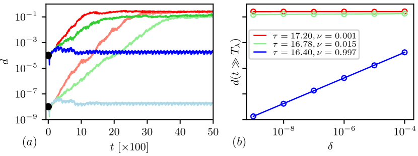
Figure 29: The evolution of the distance $d=d(t)$ between pairs of trajectories in the Mackey-Glass system (31). For each time delay $\tau$ and initial distance $\delta$ an average over $100$ pairs has been performed. ($a$) For initial distances $\delta=10^{-8}$ (light colors) and $\delta=10^{-4}$ (dark colors), as marked by black bullets. For PPC ($\tau=16.78$, green) and classical chaos ($\tau=17.20$, red), the distance grows exponentially as a function of time $t$, with the saturation plateau $d(t\to\infty)\sim\sigma$ being of order of the attractor size $\sigma$, independently of the initial distance $\delta$. For regular motion ($\tau=16.40$, blue), the long-term distance depends on the initial separation $\delta$. ($b$) Log-log plot of the long-term distance plateau $d(t\!\gg\!T_{\lambda})$ as a function of the initial separation $\delta$, with the lines corresponding to linear fits. The dependence is linear for regular motion (blue), being near to constant on the other side for both partially predictable (green) and classical chaos (red).

3.9.1 Cross-distance scaling exponent

In the vicinity of a chaotic attractor the divergence of two trajectories $x_{\text{o}}(t)$ and $x_{1}(t)$ with a small initial distance $d(t\!=\!0)=\delta\ll\sigma$ is exponential for $t<T_{\lambda}$. Here we have denoted with $\sigma^{2}$ the variance of the attractor. For systems characterized by attractors confined in a finite volume element of the phase space, viz when $\sigma<\infty$, the cross-distance $d(t)$ of a pair of trajectories reaches a saturation level, $d(t\!\gg\!T_{\lambda})\approx\text{const.}$, after the initial divergence.

As an example we present in Fig. 29 the evolution of the inter-trajectory distance $d(t)$ of the Mackey-Glass system (31) for different parameters and initial distances. Due to the finite size of the attractor the long-term distance is independent of the initial conditions $\delta$ for both classical and partially predictable chaos, one hence finds that $d(t\gg T_{\lambda})\sim\sigma$. This saturation is a consequence of the decorrelation of pairs of trajectories occurring in the vicinity of chaotic attractors, as discussed in Sect. 3.2.2. See also the decorrelation condition (54).

On the other hand, in the case of periodic motion, the long-term distance varies linearly with the initial distance [30], as shown in Fig. 29. Introducing the cross-distance scaling exponent $\nu$, one can summarize the scaling relation as

$$d(t\!\gg\!T_{\lambda}) \propto\delta^{\nu}\,,\qquad\text{where}\qquad\left\{\begin{array}[]{cl}\nu=1&\text{ for regular motion}\\ \nu=0&\text{ for chaos}\end{array}\right.$$ (80)

The scaling exponent attains in general only two values, $\nu\in\{0,1\}$, qualifying hence as a binary indicator for chaos and, respectively, for regular motion, as evident from Fig. 29. Binary classification using (80) works also for hyperchaos (cf. Table 4).

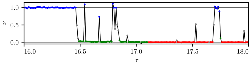
Figure 30: The cross-distance scaling exponent $\nu$ (80) for the Mackey-Glass system (31). The exponent distinguishes in a binary manner regular motion ($\nu\approx 1$, blue), when changing the time delay $\tau$, from chaos ($\nu\approx 0$, green, red). A sharp drop marks the transition from regular motion (blue) to partially predictable chaos (green). The exponents are obtained by fitting the long-term inter-pair distance plateaus as a function of the initial distances $\delta$, with $\delta\in[10^{-9},10^{-4}]$, when averaged over $100$ pairs of trajectories (cf. Fig. 29).

The binary character of the cross-distance scaling exponent can be seen also in the parameter scan presented in Fig. 30. The scaling exponent $\nu$ allows therefore to determine the transition between regular motion and chaos, as well as the presence of periodic windows.

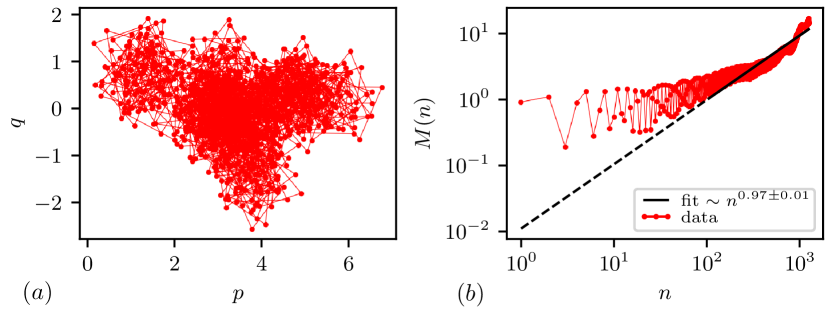
Figure 31: The Gottwald-Melbourn $0-1$ test for a chaotic attractor of the Mackey-Glass system (31) with $\tau=17.20$, using $\phi_{n}=x(t_{n})$ (extracted from $10^{3}$ points sampled with step size $t_{n+1}-t_{n}=10$) as the driving time series for the measuring device (81). Here $\zeta=2$. ($a$) The motion in phase space $p,\,q$ resembles a diffusive process. ($b$) Log-log plot of the mean-square deviation $M$, as defined by (82), as function of $n$. The close to linear growth exponent $K\approx 0.97$ correctly indicates chaotic motion.

3.9.2 Gottwald-Melbourn test

For the Gottwald-Melbourne test one uses a time series characterizing the attractor under consideration to drive a dynamical system, which serves hence as a ‘measuring device’ [193, 194]. We discuss here the case of a scalar time series $\{\phi_{j}\}_{1\leq j\leq N}$, which may be extracted, e. g., form a scalar projection of a given trajectory. This time series is used to drive the evolution of a two-dimensional mapping:

$$p(n+1) =p(n)+\phi_{n}\cos(n\zeta)\,,\qquad q(n+1)=q(n)+\phi_{n}\sin(n\zeta)\,,$$ (81)

where $\zeta>0$ corresponds to a constant angular velocity and $p$ and $q$ to the map coordinates. Of interest is the mean-square displacement (MSD)

$$M(n) =\lim\limits_{N\to\infty}\frac{1}{N}\sum\limits_{j=1}^{N}\Big{(}\big{(}p(j+n)-p(j)\big{)}^{2}+\big{(}q(j+n)-q(j)\big{)}^{2}\Big{)}\,,$$ (82)

which reflects the properties of the driving time series through the mapping (81). It has been proposed [193, 194], that the MSD is constant when the driving time series describes regular motion, growing on the other hand linearly with $n$ for irregular behavior. This would imply the binary growth rate

$$K =\lim\limits_{n\to\infty}\frac{\log M(n)}{\log n}=\left\{\begin{array}[]{cl}0&\text{ for regular motion}\\ 1&\text{ for chaotic motion}\end{array}\right.\,.$$ (85)

As an example we present in Fig. 31 the $p,\,q$ phase plane plot together with the MSD, the latter as function of iteration number $n$, for a chaotic attractor of the Mackey-Glass system (31). The representation in the phase space of the ‘measuring device’ (81) resembles a diffusion process. From a linear fit to the MSD in Fig. 31 one obtains a close to linear growth rate $K\approx 1$, which correctly indicates chaotic motion.

The Gottwald-Melbourne test is an interesting approach, which can be used at times to effectively identify chaos in time delay systems [195]. It is however also known to yield ambiguous results in some particular cases [196, 30]. The results presented for different attractors of the Mackey-Glass system in Table 4 yield correct results for periodic motion, classical chaos and hyperchaos. Though for PPC the results are ambiguous, which might hint at an insufficient, i. e. too fine, sampling rate (see also [197]).

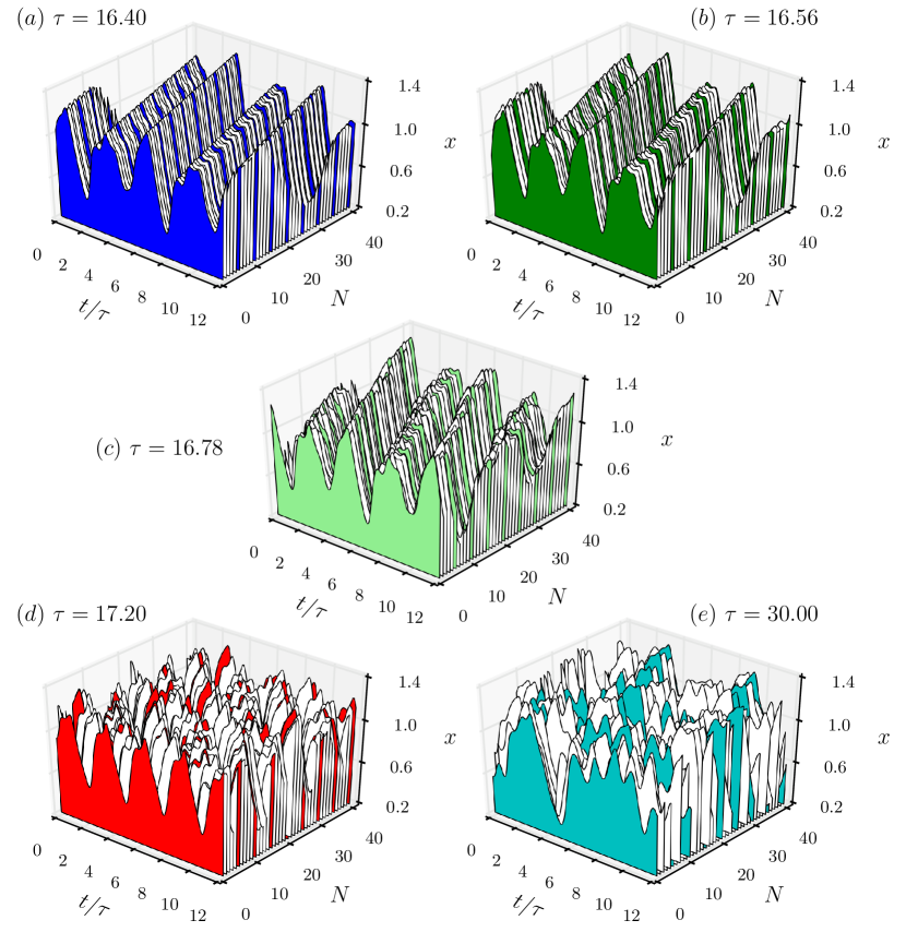
Figure 32: Space-time representation of the Mackey-Glass system (31) for different values of the delay time $\tau$ following [33]. In each panel a single trajectory $x(t)$ corresponding to an attractor is split along the time axis $t$ into $40$ slices and numbered by the quasi special dimension $N$, see (86). Time is rescaled by the delay time $\tau$ and every fifth slice is colored for better visibility. Shown is ($a$) a periodic orbit for $\tau=16.40$, ($b$) and ($c$) partially predictable chaos for $\tau=16.56$ and $\tau=16.78$, ($d$) classical chaos for $\tau=17.20$ and ($e$) hyperchaos for $\tau=30.00$.

3.10 Space-time interpretation of time delay systems

Time delay systems of scalar variables can be interpreted in terms of two-dimensional space-time coordinates [33], a visualization technique that helps at times when investigating complex dynamical patterns [34]. Within this approach, a scalar trajectory $x(t)$ is cut into slices,

$$X(N)=\{x(t)\,:\,t\in[NT,(N+1)T]\}\,,$$ (86)

of length $T$, which is usually assumed to be a multiple of the time delay $\tau$. Each point of the trajectory $X(N,t)=x(NT+t)$ is parametrized by the slicing index $N$ and the time $t\in[0,T]$ within one slice.

In Fig. 32 the space-time representation of a limit cycle and of partially predicable and classical chaotic states are shown together with a hyperchaotic trajectory of the Mackey-Glass system (31). The periodic motion appears as perfectly regular wave fronts, with PPC showing slight modulations. For classical chaotic and hyperchaotic motion, the space-time representation is instead irregular.

The space-time representation allows for regularities or irregular patterns to be identified by visual inspections. Thus, it is used to analyze pulse trains from laser cavities [198], spatio-temporal pattern formation in systems with multiple delays [66], and for the identification of chimera states in time delay systems [122].

4 Numerical treatment

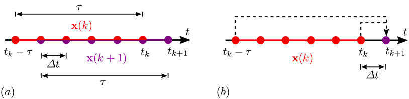
Figure 33: ($a$) Illustration of the discretized state history $\mathbf{x}(k)$ that approximates the history of a time delay system on the interval $t\in[t_{k}-\tau,t_{k}]$, with the $N>0$ steps being equidistantly spaced in time by $\varDelta t$. ($b$) The Euler algorithm for the numerical integration (91) approximates the next state $x(t_{k+1})$ combining the information of the first and last state in the state history $\mathbf{x}(k)$.

In this section, which is concerned with the numerical treatment of delay differential equations (DDE), we restrict ourselves for the sake of simplicity to autonomous DDE with constant time delay $\tau>0$ and generic flow $f$,

$$\dot{x}(t) =f\big{(}x(t),x(t-\tau)\big{)}~{},$$ (87)

where $x=x(t)$ is the scalar state of the system parametrized by time $t$. For an ordinary differential equation (ODE), a state in the phase space of the system determines the time evolution uniquely. Discretizing time, the full information about a system with fixed time delay $\tau$ at time $t=t_{k}$ is contained in contrast in the system’s state history, i. e. the states $x(t)$ on the whole interval $t\in[t_{k}-\tau,t_{k}]$. A discretization into $N>0$ equally spaced time steps, i. e. $N-1$ time intervals, therefore leads to a step-size $\varDelta t=\tau/(N-1)$, with the discretized state history taking the form

$$\mathbf{x}(k) =\left\{x(t_{k}-\tau),x(t_{k}-\tau+\varDelta t),\ldots,x(t_{k}-\varDelta t),x(t_{k})\right\}$$ (88)

$$=\{x_{\text{o}}(k),x_{1}(k),\ldots,x_{N-2}(k),x_{N-1}(k)\}\,.$$ (89)

Note that we used capital letters in Sect. 1.3 to denote state histories which are not discrete, like in (88), but continuous in time. The subscript index of $x_{j}$ indicates $x_{j}$ is the $j$th element of a vector, namely that $\mathbf{x}\in\mathbb{R}^{N}$

Two consecutive discretized time steps are linked by $t_{k+1}=t_{k}+\varDelta t$, which implies that the state history vectors $\mathbf{x}(k)$ and $\mathbf{x}(k+1)$ differ only with respect to the last element $x(t_{k+1})$ (cf. Fig. 33).

4.1 Numerical integration

Numerical methods approximate the exact solution $\hat{x}(t)$ of an DDE that is determined by an initial function $\varphi(t)$ given on the time interval $t\in[t_{k}-\tau,t_{k}]$ by a discrete set of points $\{x(t_{k}),x(t_{k+1}),\ldots\}$ for time instances $\{t_{k},t_{k+1},\ldots\}$ [179, 199]. At every integration step one can estimate the local numerical error $\lvert x(t_{k})-\hat{x}(t_{k})\rvert$, which will generally depend on the discretization step size $\varDelta t$.

For the purpose of numerical integration the state vector $\mathbf{x}(k)$ is updated to the next state vector $\mathbf{x}(k+1)$, as illustrated in Fig. 33. The challenge lies in the discretized nature of the state history, which may not contain the states $x(t)$ at the times $t$ a given integration algorithm may need when calculating the new element $x(t_{k+1})$.

4.1.1 Euler algorithm

The Euler integration algorithm uses the simplest numerical approximation of the time derivative occurring in a differential equation,

$$\dot{x}(t) =\lim\limits_{\varDelta t\to 0}\frac{x(t+\varDelta t)-x(t)}{\varDelta t}\approx\frac{x(t+\varDelta t)-x(t)}{\varDelta t}\,.$$ (90)

This approximation implies that

$$x(t_{k+1}) =x(t_{k})+F\big{(}x(t_{k}),x(t_{k}-\tau)\big{)}\varDelta t~{},$$ (91)

which requires the system’s state at the previous time step $x(t_{k})$ and the delayed state $x(t_{k}-\tau)$ (cf. Fig. 33). Thus, for the Euler integration algorithm the discretization step size $\varDelta t$ and the delay $\tau$ must be commensurate, which is in accordance with the choice $\tau=(N-1)\varDelta t$.

From the approximation (90) of the time derivative the local numerical error is $\mathcal{O}(\varDelta t^{2})$. The cumulative error of the Euler method when integrating up successively to a finite time difference is however $\mathcal{O}(\varDelta t)$, which determines the overall numerical accuracy.

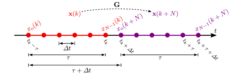
Figure 34: The Euler map $G$, as defined by Eqs. (92) and (93), maps the state history $\mathbf{x}(k)$ onto the disjoint state history $\mathbf{x}(k+N)$. Both state histories contain the discretized states over a time span of length $\tau$, but shifted by $\tau+\varDelta t$ with respect to each other.

4.1.2 Euler integration as a discrete map

As described by [47], one can interpret the Euler algorithm (91) as the discrete map

$$\mathbf{x}(k+N) =\mathbf{G}\big{(}\mathbf{x}(k)\big{)}\,,$$ (92)

where the map $\mathbf{G}\,:\,\mathbb{R}^{N}\to\mathbb{R}^{N}$ maps the state history $\mathbf{x}(k)$ of $N$ time steps of size $\varDelta t$, i. e. with $N\varDelta t=\tau+\varDelta t$, onto the disjoint state history $\mathbf{x}(k+N)$. At first sight this approach, which is depicted in Fig. 34, seems arbitrary, but is has the advantage of being an explicit forward recursive map once the recursive dependencies are expanded:

$$\begin{array}[]{rcll}x_{\text{o}}(k+N)&=&x_{N-1}(k)&+\,\varDelta t\,F\big{(}x_{N-1}(k),x_{\text{o}}(k)\big{)}\\[2.15277pt] x_{1}(k+N)&=&x_{\text{o}}(k+N)&+\,\varDelta t\,F\big{(}x_{\text{o}}(k+N),x_{1}(k)\big{)}\\[2.15277pt] &\vdots&\\[2.15277pt] x_{N-1}(k+N)&=&x_{N-2}(k+N)&+\,\varDelta t\,F\big{(}x_{N-2}(k+N),x_{N-1}(k)\big{)}\,.\end{array}$$ (93)

Note the implicit recursion, namely that the RHS of $x_{1}(k+N)$ depends on $x_{\text{o}}(k+N)$, and so on.

As an illustrative example we consider as in Sect. 1.5 the integration of $\dot{x}(t)=-x(t-\tau)$, here with step size $\varDelta t=\tau/2$, which corresponds to $N=3$ steps per state history. The state history therefore consists of

$$\mathbf{x}(k) =\big{\{}x_{\text{o}}(k),\;x_{1}(k),\;x_{2}(k)\big{\}}$$

$$=\big{\{}x(t_{k}-\tau),\;x(t_{k}-\tau/2),\;x(t_{k})\big{\}}~{},$$

which means for the Euler map (92) that one computes the consecutive disjoint state history

$$\mathbf{x}(k+N) =\big{\{}x_{\text{o}}(k+N),\;x_{1}(k+N),\;x_{2}(k+N)\big{\}}$$

$$=\big{\{}x(t_{k}+\tau/2),\;x(t_{k}+\tau),\;x(t_{k}+3\tau/2)\big{\}}\,.$$

The single states follow from the iterative stepwise map (93):

$$\begin{split}x_{\text{o}}(k+N)&=x_{2}(k)-\frac{\tau}{2}x_{\text{o}}(k)\\ x_{1}(k+N)&=x_{2}(k)-\frac{\tau}{2}\big{(}x_{\text{o}}(k)+x_{1}(k)\big{)}\\ x_{2}(k+N)&=x_{2}(k)-\frac{\tau}{2}\big{(}x_{\text{o}}(k)+x_{1}(k)+x_{2}(k)\big{)}\,.\end{split}$$ (94)

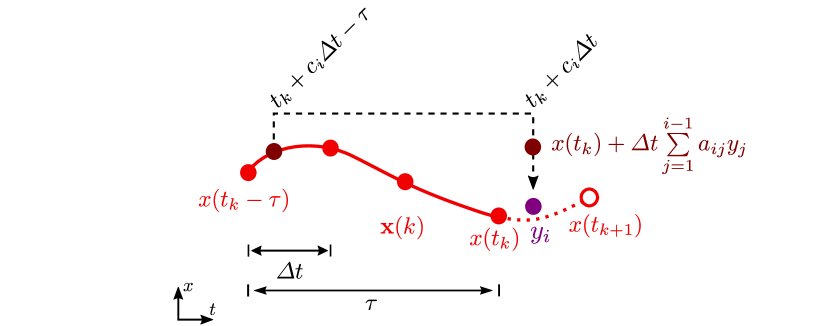
Figure 35: For a Runge-Kutta integration step (95) at $t=t_{k}$ one needs to compute the intermediate states $y_{i}$ defined by Eq. (96). The flow is hence to be evaluated at times $t_{k}+c_{i}\varDelta t$ and at corresponding estimated points in phase space. The delayed contribution $x(t_{k}+c_{i}\varDelta t-\tau)$ to the flow are obtained correspondingly by interpolating the state history $\mathbf{x}(k)$.

4.1.3 Explicit Runge-Kutta algorithms

The trade-off between the integration step size and the numerical error makes the explicit Euler integration algorithm either slow or inaccurate. Its generalization is referred to as explicit Runge-Kutta (RK) algorithms [200, 201, 202]. Explicit RK algorithms use $s>0$ intermediate sampling points $y_{i}$ to estimate the next state,

$$x(t_{k+1}) =x(t_{k})+\varDelta t\sum\limits_{i=1}^{s}b_{i}y_{i}~{},$$ (95)

where the coefficients $b_{i}>0$ are weighting factors for the sampling points. They are computed for $\dot{x}(t)=f(t,x(t),x(t-\tau))$ iteratively as

$$y_{i} =f\left(t_{k}+c_{i}\varDelta t,\;x(t_{k})+\varDelta t\sum\limits_{j=1}^{i-1}a_{ij}y_{j},\;x(t_{k}+c_{i}\varDelta t-\tau)\right)\,.$$ (96)

The flow $f$ is hence evaluated at time instances $t_{k}+c_{i}\varDelta t$ in $[t_{k},t_{k+1}]$, which are determined in turn by the coefficients $0\leq c_{i}\leq 1$, with the state argument of the flow being a superposition of previous intermediate stages, as weighted by the coefficients $a_{ij}$.

The times at which the $y_{i}$ are to be evaluated, $t_{k}+c_{i}\varDelta t$, are in general incommensurate with the underlying time discretization, as illustrated in Fig. 35, which means that the state history $\mathbf{x}(k)$ needs to interpolated [203]. However, the advantage is that an $s$ stage RK algorithm comes with a global numerical error of the order $\mathcal{O}(\varDelta t^{p})$ with $p\leq s$, allowing such for a faster and/or more accurate integration compared to the straightforward Euler method.

The coefficients $a_{ij},b_{i},c_{i}$ for the explicit RK algorithms are usually written as a ‘Butcher tableau’ [204]:

$$\begin{array}[]{c|cccccc}c_{1}=0&0&\lx@intercol\hfil\dots\hfil\lx@intercol&0\\ c_{2}&a_{21}&0\\ c_{3}&a_{31}&a_{32}&0&&\vdots\\ \vdots&\vdots&&\ddots&\ddots\\ c_{s}&a_{s1}&a_{s2}&\dots&a_{s,s-1}&0\\ \hline\cr&b_{1}&b_{2}&\dots&b_{s-1}&b_{s}\end{array}$$ (97)

where the upper triangle contains only zeros for explicit RK algorithms. The so-called 3/8 rule [201] is a fourth order ($s=4$) Runge-Kutta method has the Butcher tableau:

$$\begin{array}[]{c|cccc}0\\ \nicefrac{{1}}{{3}}&\phantom{-}\nicefrac{{1}}{{3}}\\ \nicefrac{{2}}{{3}}&-\nicefrac{{1}}{{3}}&\phantom{-}1\\ 1&\phantom{-}1&-1&1\\ \hline\cr&\phantom{-}\nicefrac{{1}}{{8}}&\phantom{-}\nicefrac{{3}}{{8}}&\nicefrac{{3}}{{8}}&\nicefrac{{1}}{{8}}\end{array}$$ (98)

It is appreciated for its stability and convergence properties [201].

4.2 Lyapunov exponents

Lyapunov exponents describe the contraction or expansion of phase space volume associated with certain directions in phase space, or on an attractor in particular. While for an ordinary differential equation there is only a finite number of Lyapunov exponents, which equals the number of dimensions of the phase space, a time delay system has infinitely many Lyapunov exponents. In consequence one can only approximate the $N$ largest exponents (largest by real part) with numerical methods. In the following three different commonly used numerical methods for computing the largest or the $N$ largest Lyapunov exponents are discussed.

Note that the methods for evaluating Lyapunov exponents presented in this section are suited for smooth systems. For non-smooth dynamical systems one typically needs dedicated approaches [205, 206], which holds also for time delay systems [187].

4.2.1 Maximal Lyapunov exponent from two diverging trajectories

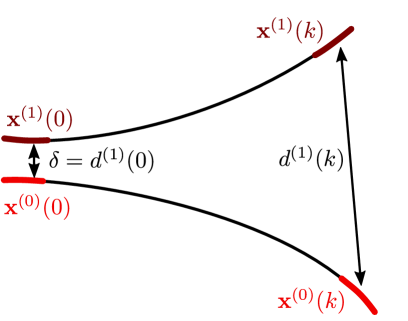
Figure 36: Measuring the rate of divergence of two trajectories starting at initial states $\mathbf{x}^{(0)}(0)$ and $\mathbf{x}^{(1)}(0)$ with an initial distance $d^{(1)}(0)=\delta$ (cf. Eq. (100)). The distance $d^{(1)}(k)$ after $k$ integration steps is used to compute the Lyapunov exponent via (101). The thick segments of length $\tau$ indicate the respective state histories.

The most basic method of determining Lyapunov exponents implies measuring the divergence rate of initially close-by trajectories [30]. For the maximal Lyapunov exponent $\lambda_{\text{max}}=\lambda_{1}$ two initial state histories $\mathbf{x}^{(0)}(0)=\left\{x^{(0)}_{\text{o}}(0),\ldots,x^{(0)}_{N-1}(0)\right\}$ and $\mathbf{x}^{(1)}(0)$ at $t=t_{\text{o}}$ are chosen and evolved for $k>0$ steps, until $t_{k}=t_{\text{o}}+k\varDelta t$, to states $\mathbf{x}^{(0)}(k)$ and $\mathbf{x}^{(1)}(k)$, cf. Fig. 36.

At every time step $t_{k}$ one can define the difference vector between the two state history vectors,

$$\mathbf{d}^{(1)}(k)=\mathbf{x}^{(1)}(k)-\mathbf{x}^{(0)}(k)~{},$$ (99)

from which one can compute the average Euclidean distance of the state history vectors, namely

$$d^{(1)}(k) =\frac{\lVert\mathbf{d}^{(1)}(k)\rVert}{\sqrt{N}}=\left(\frac{1}{N}\sum\limits_{i=0}^{N-1}\left(x_{i}^{(0)}(k)-x_{i}^{(1)}(k)\right)^{2}\right)^{1/2}\,.$$ (100)

In contrast to the Euclidean distance between continuous state history vectors, as defined in Sect. 1.3, the average distance defined by (100) does not diverge in the limit $N\to\infty$. Note also that we adapted the notation in order to emphasis that we are working in this section with discrete and not with continuous state histories.

The initial states $\mathbf{x}^{(0)}(0)$ and $\mathbf{x}^{(1)}(0)$ are normally chosen randomly in the vicinity of the attractor under investigation, with the initial distance $d^{(1)}(0)=\delta$ being small, $\delta\ll\sigma$, with respect to the variance $\sigma^{2}$ of the attractor. If $\sigma=0$, as for a fixed point, the initial distance should be small with respect to the microscopic length scales of the system. The maximal Lyapunov exponent $\lambda_{\text{max}}$ is given, as pointed out in Sect. 1.4.2, by the divergence rate of the two trajectories,

$$\lambda_{\text{max}} =\lim\limits_{k\to\infty}\lim\limits_{\delta\to 0}\frac{1}{k\varDelta t}\log\frac{d^{(1)}(k)}{\delta}\,,$$ (101)

where the limit of infinitely small initial distances $\delta\to 0$ and the long-term limit for the measurement time $k\varDelta t$ needs to be taken. For chaotic attractors, for which pairs of trajectories eventually decorrelate, one has that $d^{(1)}(k)\to\sigma$ in the limit $k\to\infty$ [30]. The maximal Lyapunov exponent has to be evaluated accordingly for intermediate distances $d^{(1)}$, as defined by $\delta\ll d^{(1)}\ll\sigma$.

This expression, Eq. (101), is an intuitive and robust method, it allows however to determine only a single Lyapunov exponent, namely the maximal Lyapunov exponent. An extension to compute the $N$ largest Lyapunov exponents is discussed in the following section.

4.2.2 Benettin’s algorithm

The largest Lyapunov exponents can be evaluated efficiently following the idea of Benettin et al [44], which is widely used and illustrated, e. g. in [45]. Here we discuss two different aspects of Benettin’s algorithm.

Iterated finite-time method

Instead of measuring the divergence of one pair of trajectories for large times, one can rely on iterated measurements of the rate of divergence for shorter time intervals. Within this approach one computes a reference trajectory $\mathbf{x}^{(0)}$ starting at a random initial condition $\mathbf{x}^{(0)}(0)$ in the vicinity of the attractor. The initial condition $\mathbf{x}^{(1)}(0)$ for the auxiliary trajectory $\mathbf{x}^{(1)}$ is chosen such that the initial distance is $d^{(1)}(0)=\delta\ll\sigma$ is small compared to the extent $\sigma$ (or the variance $\sigma^{2}$) of the attractor under investigation. The divergence of both trajectories is measured by their distance $d^{(1)}(k)$ after $k$ integration steps, viz after an integration time $k\varDelta t$. The finite-time Lyapunov exponent,

$$\lambda_{1}^{(\text{ft})}=\frac{1}{k\varDelta t}\log\frac{d^{(1)}(k)}{\delta}~{},$$ (102)

then provides a local estimate of (101). Next one rescales the auxiliary vector $\mathbf{x}^{(1)}(k)$ to $\tilde{\mathbf{x}}^{(1)}(k)$, such that the distance to the reference trajectory is reset to

$$\lVert\tilde{\mathbf{x}}^{(1)}(k)-\mathbf{x}^{(0)}(k)\rVert=\sqrt{N}\delta\,.$$ (103)

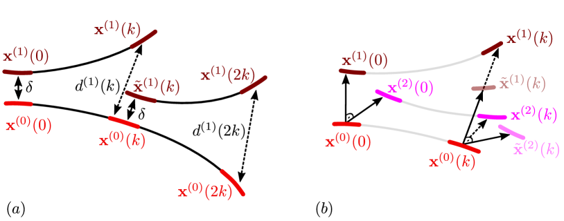
Figure 37: Estimating Lyapunov exponents using Benettin’s method. ($a$) Iteratively measuring the distance $d^{(1)}$ between the reference trajectory $\mathbf{x}^{(0)}$ and the auxiliary trajectory $\mathbf{x}^{(1)}$. After each iteration the auxiliary state is rescaled, such that the initial distance $d^{(1)}=\delta$ is restored. ($b$) Computing the $L=2$ largest Lyapunov exponents using a reference trajectory $\mathbf{x}^{(0)}$ and two auxiliary trajectories $\mathbf{x}^{(1)}$ and $\mathbf{x}^{(2)}$, in the same way as shown in ($a$). The set of difference vectors are initially selected to be orthogonal, and re-orthogonalized and rescaled after every step of the iteration. The thick segments of length $\tau$ indicate the respective state histories.

The procedure described above is repeated with $\mathbf{x}^{(0)}(k)$ and $\tilde{\mathbf{x}}^{(1)}(k)$ being the new pair of starting state histories, cf. Fig. 37. After $M$ iterations the average of the finite time Lyapunov exponents

$$\langle\lambda_{1}^{(\text{ft})}\rangle =\frac{1}{M}\sum\limits_{j=1}^{M}\frac{1}{k\varDelta t}\log\left(\frac{d^{(1)}(j\cdot k)}{\delta}\right)\approx\lambda_{1}\quad\qquad(M\to\infty)$$ (104)

then converges to the largest Lyapunov exponent $\lambda_{1}$. Of interest in this context is that the distribution of local finite-time Lyapunov exponents can have a variance that is large compared to the average value [30].

Keeping the direction of the difference vector $\mathbf{d}^{(1)}(k)$ in every iteration ensures that $\mathbf{d}^{(1)}(k)$ aligns with the direction of the largest divergence in phase space. Note that this is not a fixed direction, but a direction that depends on the location on the attractor. For a given system the integration step size $\varDelta t$, the number of steps $k$ during divergence, the initial distance $\delta$ and the number of iterations $M$ have to be optimized.

Computing arbitrary many exponents

The iterated method of diverging trajectories allows also to compute, when suitably generalized, the $L\leq N$ largest exponents. In this context the trajectory $\mathbf{x}^{(0)}$ serves as reference for a set of $L$ auxiliary trajectories of state histories, $\left\{\mathbf{x}^{(1)},\ldots,\mathbf{x}^{(L)}\right\}$. The initial conditions $\mathbf{x}^{(i)}(0)$ of the auxiliary trajectories are selected such that their distance to the reference state history $\mathbf{x}^{(0)}(0)$ is small, $d^{(i)}(0)=\delta$, with the difference vectors with respect to the reference point being mutually orthogonal:

$$\mathbf{d}^{(i)}(0)\cdot\mathbf{d}^{(j)}(0) =\left\{\begin{array}[]{cl}N\delta^{2}&\text{ if }\;i=j\\ 0&\text{ else}\end{array}\right.\,.$$ (107)

From the distances $d^{(i)}(k)$ after $k$ integration steps the local Lyapunov exponents $\lambda_{i}^{(\text{ft})}$ are estimated following (102). In order to prepare the next iteration, the first reference state is rescaled $\mathbf{x}_{1}(k)\to\tilde{\mathbf{x}}_{1}(k)$ according to (103). The remaining reference states are then modified, such that all $L$ difference vectors form an orthogonal set with each vector having an average length $d^{(i)}(k)=\delta$. This procedure is sketched in Fig. 37 for $L=2$. Performing the iteration $M$ times allows then to estimate the average Lyapunov exponents $\langle\lambda_{i}^{(\text{ft})}\rangle$ via Eq. (104).

Using in every time step an iterative algorithm for the orthogonalization, such as the Gram-Schmidt procedure, ensures that the $i$th difference vector aligns with the $i$th direction of divergence and that the average Lyapunov exponents $\langle\lambda_{\text{max}}^{(\text{ft})}\rangle=\langle\lambda_{1}^{(\text{ft})}\rangle\geq\langle\lambda_{2}^{(\text{ft})}\rangle\geq\ldots\geq\langle\lambda_{L}^{(\text{ft})}\rangle$ are ordered [207, 208].

Benettin’s method is widely used for the evaluation of the Lyapunov spectrum of a dynamical system. Its accuracy is limited however in particular by the numerical restrictions arising from the Gram-Schmidt orthogonalization procedure. Alternative concepts for addressing the Lyapunov exponents and the corresponding directional vectors are consequently of interest [139].

4.2.3 Extracting Lyapunov exponents from the Euler map

Lyapunov exponents may be extracted, as mentioned already in Sect. 1.4.3, also from the discretized system (92), viz from the Euler map $\mathbf{x}(k+N)=\mathbf{G}(\mathbf{x}(k))$, where $G$ is a $N\times N$ matrix. The respective Jacobian matrix of derivatives $J(k)=\left\{J_{lm}(k)\right\}$ evaluated for a state $\mathbf{x}(k)$ of the map (92),

$$J_{lm}(k) =\frac{\partial G_{l}\big{(}\mathbf{x}(k)\big{)}}{\partial x_{m}(k)},\qquad\quad 0\leq l,m<N~{},$$ (108)

has $N$ complex eigenvalues $\sigma_{j}(k)\equiv\sigma_{j}=\sigma_{j}^{\prime}+\imath\sigma_{j}^{\prime\prime}$, with real and imaginary parts $\sigma_{j}^{\prime}$ and $\sigma_{j}^{\prime\prime}$, that describe the dynamics of the Euler mapping (92) in tangent space [42, 48]. We now consider with

$$\mathbf{d}^{(1)}(k)=\mathbf{x}^{(1)}(k)-\mathbf{x}^{(0)}(k)=\delta\,\mathbf{e}_{j}(k)$$ (109)

two state vectors $\mathbf{x}^{(0)}(k)$ and $\mathbf{x}^{(1)}(k)$ for which the distance vector $\mathbf{d}^{(1)}(k)$ is aligned to the $j$th (normalized) eigenvector $\mathbf{e}_{j}(k)$ of the Jacobian $J$ of the Euler map. The Jacobian maps this distance vector to $J\mathbf{d}^{(1)}(k)=\delta\sigma_{j}\mathbf{e}_{j}(k)$, viz to a vector having the norm

$$\lVert J(k)\,\mathbf{d}^{(1)}(k)\rVert=\lVert\delta\,\sigma_{j}(k)\,\mathbf{e}_{j}(k)\rVert=\delta\,\lVert\sigma_{j}(k)\rVert\,.$$ (110)

It is known that the local Lyapunov exponents of a map equal the logarithm of the eigenvalues of the corresponding Jacobian matrix [40]. For the Euler map the logarithm of the Jacobian’s eigenvalues $\sigma_{j}$ converges for $N\to\infty$ to the local Lyapunov exponents $\Lambda_{j}$ of the approximated DDE:

$$\frac{1}{\tau}\log\sigma_{j}\to\Lambda_{j}\quad\text{ for }N\to\infty\,,\qquad\sigma_{j}=\lVert\sigma_{j}\rVert\;\exp(\imath\arg\sigma_{j})\,,$$ (111)

where $\arg\sigma_{j}$ denotes the argument of a complex number, which corresponds to its phase angle in polar representation. The normalization factor $1/\tau$ in Eq. (111) stems from the fact that the Euler map evolves by a time difference of $\tau$ in every iteration.

One may thus use the modulus $\lVert\sigma_{j}(k)\rVert$ of the $j$th eigenvalue of the Jacobian of the Euler map to approximate the real part $\Lambda_{j}^{\prime}$ of the local Lyapunov exponent at a point in phase space, which corresponds to the state $\mathbf{x}(k)$ of the Euler map (92):

$$\Lambda^{\prime}_{j} =\lim\limits_{N\to\infty}\frac{1}{\tau}\log\lVert\sigma_{j}(k)\rVert\,,\qquad\lVert\sigma_{j}\rVert^{2}=(\sigma_{j}^{\prime})^{2}+(\sigma_{j}^{\prime\prime})^{2}\,,$$ (112)

compare Eq. (27).

5 Conclusions

Dynamical systems with retarded interactions constitute an active and rapidly developing research field with increasing relevance for real-world applications. An example is the proposal [58], that the time delays resulting from entrenched election cycles may contribute to destabilizing modern democracies, in particular if the presumption holds that the technological progress induces a continuously accelerating opinion dynamics.

A defining feature of time delay system is the enlarged phase space, which becomes formally infinite-dimensional when retarded feedback is introduced into a finite dimensional dynamical system. The existence of an infinitely large phase space, the space of state histories, raises a series of interesting questions, as pointed out in the introduction, Sect. 1, such as: How to treat an infinite dimensional system and it’s diverging spectrum of Lyapunov exponents? How does the phase space compactify in the limit of vanishing time delays?

Time delays come in large varieties, as detailed out systematically in Sect. 2, one of the fascinating aspects of the field. The possibilities range here from time delays that are characterized by their dependence on time, on the state, or by a statistical distribution. Time delays may be classified furthermore by alternative criteria, such as being conservative or dissipative.

The distinct types of time delays lead to a corresponding large range of dynamical behaviors, as discussed in Sect. 3, in particular for chaotic states, the central theme of this review. Chaos may be classical or partially predictable, weak or strong, intermittent or laminar. Of particular importance in this respect are binary tests for chaos, which we also included in Sect. 3. There exists furthermore a range of complementing proposals for the dimension of a chaotic attractor, for which we discussed the respective implementations for time delay systems.

Numerical simulations of time delay systems is generally demanding, as explained in Sect. 4, as a consequence of the formally diverging dimension of the phase space of state histories. A central algorithm for the evaluation of the spectrum of global Lyapunov exponents is here Benettin’s method, but it is also of interest, as we point out in Sect. 4, to cross-check with the results obtained from the Euler map.

Overall we hope that this review serves its purpose as a concise compendium of the state of the field that provides in addition tools for a comprehensive classification of time delay systems and of the respective induced types of chaotic dynamics. We interseeded the discussion with several educational examples aiming to provide a self-contained presentation of the material. Our intention is that this comprehensive review may also serve as an entry points for both practitioners and newcomers to the field.

6 Competing interests

The authors declare that they have no competing interests.

7 Funding

This research was funded by the German research foundation (DFG). H. W. acknowledges the financial support from Stiftung Polytechnische Gesellschaft Frankfurt am Main.

8 Authors’ contributions

The paper was mostly written by H. W. and C. G., B. S. adding some paragraphs and contributing to the analytical derivations and numerical methods part. H. W. did all simulations and prepared all figures. All authors reviewed the manuscript.

References

References

- [1] W. Just, A. Pelster, M. Schanz, E. Schöll, Delayed complex systems: an overview (2010).
- [2] T. Erneux, J. Javaloyes, M. Wolfrum, S. Yanchuk, Introduction to Focus Issue: Time-delay dynamics, Chaos: An Interdisciplinary Journal of Nonlinear Science (114201).
- [3] M. C. Soriano, J. García-Ojalvo, C. R. Mirasso, I. Fischer, Complex photonics: Dynamics and applications of delay-coupled semiconductors lasers, Reviews of Modern Physics 85 (1) (2013) 421.
- [4] L. Larger, M. C. Soriano, D. Brunner, L. Appeltant, J. M. Gutiérrez, L. Pesquera, C. R. Mirasso, I. Fischer, Photonic information processing beyond Turing: an optoelectronic implementation of reservoir computing, Optics express 20 (3) (2012) 3241–3249.
- [5] J. Houlihan, D. Goulding, T. Busch, C. Masoller, G. Huyet, Experimental investigation of a bistable system in the presence of noise and delay, Physical Review Letters 92 (5) (2004) 050601.
- [6] C. Masoller, Noise-induced resonance in delayed feedback systems, Physical Review Letters 88 (3) (2002) 034102.
- [7] A. Payeur, L. Maler, A. Longtin, Oscillatorylike behavior in feedforward neuronal networks, Physical Review E 92 (1) (2015) 012703.
- [8] H. U. Voss, Anticipating chaotic synchronization, Physical Review E 61 (5) (2000) 5115.
- [9] C. Masoller, Anticipation in the synchronization of chaotic semiconductor lasers with optical feedback, Physical Review Letters 86 (13) (2001) 2782.
- [10] M. Ciszak, O. Calvo, C. Masoller, C. R. Mirasso, R. Toral, Anticipating the response of excitable systems driven by random forcing, Physical Review Letters 90 (20) (2003) 204102.
- [11] K. Pyragas, Continuous control of chaos by self-controlling feedback, Physics Letters A 170 (6) (1992) 421–428.
- [12] E. Schöll, H. G. Schuster, Handbook of chaos control, John Wiley & Sons, 2008.
- [13] N. B. Janson, A. G. Balanov, E. Schöll, Delayed feedback as a means of control of noise-induced motion, Physical Review Letters 93 (1) (2004) 010601.
- [14] J. Foss, A. Longtin, B. Mensour, J. Milton, Multistability and delayed recurrent loops, Physical Review Letters 76 (4) (1996) 708.
- [15] J. Foss, J. Milton, Multistability in recurrent neural loops arising from delay, Journal of Neurophysiology 84 (2) (2000) 975–985.
- [16] N. MacDonald, T. Lags, Lecture notes in biomathematics, Springer, 1978.
- [17] G. Stepan, Delay effects in brain dynamics, Phil. Trans. R. Soc. A 367 (2009) 1059–1062.
- [18] B. Rahman, K. B. Blyuss, Y. N. Kyrychko, Dynamics of neural systems with discrete and distributed time delays, SIAM Journal on Applied Dynamical Systems 14 (4) (2015) 2069–2095.
- [19] G. Deco, V. Jirsa, A. R. McIntosh, O. Sporns, R. Kötter, Key role of coupling, delay, and noise in resting brain fluctuations, Proceedings of the National Academy of Sciences (2009) pnas–0901831106.
- [20] J. Martínez-Llinàs, X. Porte, M. C. Soriano, P. Colet, I. Fischer, Dynamical properties induced by state-dependent delays in photonic systems, Nature Communications 6 (2015) 7425.
- [21] T. Insperger, G. Stépán, F. Hartung, J. Turi, State dependent regenerative delay in milling processes, in: ASME 2005 International Design Engineering Technical Conferences and Computers and Information in Engineering Conference, American Society of Mechanical Engineers, 2005, pp. 955–964.
- [22] D. Bachrathy, G. Stépán, J. Turi, State dependent regenerative effect in milling processes, Journal of Computational and Nonlinear Dynamics 6 (4) (2011) 041002.
- [23] P. Hövel, Control of complex nonlinear systems with delay, Springer Science & Business Media, 2010.
- [24] E. Stone, S. A. Campbell, Stability and bifurcation analysis of a nonlinear DDE model for drilling, Journal of Nonlinear Science 14 (1) (2004) 27–57.
- [25] A. Otto, G. Radons, Application of spindle speed variation for chatter suppression in turning, CIRP Journal of Manufacturing Science and Technology 6 (2) (2013) 102–109.
- [26] J. Milton, J. L. Cabrera, T. Ohira, S. Tajima, Y. Tonosaki, C. W. Eurich, S. A. Campbell, The time-delayed inverted pendulum: implications for human balance control, Chaos: An Interdisciplinary Journal of Nonlinear Science 19 (2) (2009) 026110.
- [27] J. Sieber, B. Krauskopf, Complex balancing motions of an inverted pendulum subject to delayed feedback control, Physica D: Nonlinear Phenomena 197 (3-4) (2004) 332–345.
- [28] S. A. Campbell, S. Crawford, K. Morris, Friction and the inverted pendulum stabilization problem, Journal of Dynamic Systems, Measurement, and Control 130 (5) (2008) 054502.
- [29] A. Keane, B. Krauskopf, C. M. Postlethwaite, Climate models with delay differential equations, Chaos: An Interdisciplinary Journal of Nonlinear Science 27 (11) (2017) 114309.
- [30] H. Wernecke, B. Sándor, C. Gros, How to test for partially predictable chaos, Scientific Reports 7.
- [31] D. Müller, A. Otto, G. Radons, Laminar chaos, Physical Review Letters 120 (8) (2018) 084102.
- [32] A. Otto, D. Müller, G. Radons, Universal dichotomy for dynamical systems with variable delay, Physical Review Letters 118 (4) (2017) 044104.
- [33] F. Arecchi, G. Giacomelli, A. Lapucci, R. Meucci, Two-dimensional representation of a delayed dynamical system, Physical Review A 45 (7) (1992) R4225.
- [34] S. Yanchuk, G. Giacomelli, Spatio-temporal phenomena in complex systems with time delays, Journal of Physics A: Mathematical and Theoretical 50 (10) (2017) 103001.
- [35] C. Masoller, Spatiotemporal dynamics in the coherence collapsed regime of semiconductor lasers with optical feedback, Chaos: An Interdisciplinary Journal of Nonlinear Science 7 (3) (1997) 455–462.
- [36] H. D. Abarbanel, R. Brown, M. B. Kennel, Local Lyapunov exponents computed from observed data, Journal of Nonlinear Science 2 (3) (1992) 343–365.
- [37] H. D. Abarbanel, R. Brown, M. B. Kennel, Variation of Lyapunov exponents on a strange attractor, Journal of Nonlinear Science 1 (2) (1991) 175–199.
- [38] J.-P. Eckmann, D. Ruelle, Ergodic theory of chaos and strange attractors, in: The Theory of Chaotic Attractors, Springer, 1985, pp. 273–312.
- [39] M. Lakshmanan, D. V. Senthilkumar, Delay Differential Equations, in: Dynamics of Nonlinear Time-Delay Systems, Springer, 2011, pp. 1–15.
- [40] C. Gros, Complex and adaptive dynamical systems: A primer, Springer, 2015.
- [41] G. Lapeyre, Characterization of finite-time Lyapunov exponents and vectors in two-dimensional turbulence, Chaos: An Interdisciplinary Journal of Nonlinear Science 12 (3) (2002) 688–698.
- [42] A. Pikovsky, A. Politi, Lyapunov exponents: a tool to explore complex dynamics, Cambridge University Press, 2016.
- [43] G. Károlyi, M. Pattantyús-Ábrahám, T. Krámer, J. Józsa, T. Tél, Finite-size Lyapunov exponents: A new tool for lake dynamics, Proceedings of the Institution of Civil Engineers-Engineering and Computational Mechanics 163 (4) (2010) 251–259.
- [44] G. Benettin, L. Galgani, A. Giorgilli, J.-M. Strelcyn, Lyapunov characteristic exponents for smooth dynamical systems and for Hamiltonian systems; a method for computing all of them. Part 1: Theory, Meccanica 15 (1) (1980) 9–20.
- [45] C. Skokos, The Lyapunov characteristic exponents and their computation, in: Dynamics of Small Solar System Bodies and Exoplanets, Springer, 2010, pp. 63–135.
- [46] A. Wolf, J. B. Swift, H. L. Swinney, J. A. Vastano, Determining Lyapunov exponents from a time series, Physica D: Nonlinear Phenomena 16 (3) (1985) 285–317.
- [47] J. D. Farmer, Chaotic attractors of an infinite-dimensional dynamical system, Physica D: Nonlinear Phenomena 4 (3) (1982) 366–393.
- [48] B. Sándor, The world of dynamical systems: multistability, neural dynamics and robotic locomotion, Ph.D. thesis, Goethe University Frankfurt, Institute for Theoretical Physics, Goethe University Frankfurt/Main, Germany (9 2017).
- [49] E. Ott, Chaos in dynamical systems, Cambridge University Pressversity press, 2002.
- [50] I. Shimada, T. Nagashima, A numerical approach to ergodic problem of dissipative dynamical systems, Progress of Theoretical Physics 61 (6) (1979) 1605–1616.
- [51] J. Sieber, R. Szalai, Characteristic matrices for linear periodic delay differential equations, SIAM Journal on Applied Dynamical Systems 10 (1) (2011) 129–147.
- [52] W. Just, On the eigenvalue spectrum for time-delayed Floquet problems, Physica D: Nonlinear Phenomena 142 (1-2) (2000) 153–165.
- [53] C. R. Williams, F. Sorrentino, T. E. Murphy, R. Roy, Synchronization states and multistability in a ring of periodic oscillators: Experimentally variable coupling delays, Chaos: An Interdisciplinary Journal of Nonlinear Science 23 (4) (2013) 043117.
- [54] G. D. VanWiggeren, R. Roy, Chaotic communication using time-delayed optical systems, International Journal of Bifurcation and Chaos 9 (11) (1999) 2129–2156.
- [55] B. Mensour, A. Longtin, Synchronization of delay-differential equations with application to private communication, Physics Letters-Section A 244 (1) (1998) 59–70.
- [56] R. Jiang, Q. Wu, Z. Zhu, Full velocity difference model for a car-following theory, Physical Review E 64 (1) (2001) 017101.
- [57] K. J. Lang, A. H. Waibel, G. E. Hinton, A time-delay neural network architecture for isolated word recognition, Neural networks 3 (1) (1990) 23–43.
- [58] C. Gros, Entrenched time delays versus accelerating opinion dynamics: are advanced democracies inherently unstable?, The European Physical Journal B 90 (11) (2017) 223.
- [59] M. C. Mackey, L. Glass, et al., Oscillation and chaos in physiological control systems, Science 197 (4300) (1977) 287–289.
- [60] T. Tél, M. Gruiz, Chaotic dynamics: An introduction based on classical mechanics, Cambridge University Press, 2006.
- [61] S. A. J. Marsden, L. S. S. Wiggins, L. Glass, R. Kohn, S. Sastry, Interdisciplinary Applied Mathematics, Vol. 3, Springer, 1993.
- [62] P. Grassberger, I. Procaccia, Measuring the strangeness of strange attractors, Physica D: Nonlinear Phenomena 9 (1-2) (1983) 189–208.
- [63] A. Otto, G. Radons, D. Bachrathy, G. Orosz, Synchronization in networks with heterogeneous coupling delays, Physical Review E 97 (1) (2018) 012311.
- [64] C. Masoller, A. C. Marti, Random delays and the synchronization of chaotic maps, Physical Review Letters 94 (13) (2005) 134102.
- [65] J. Stuart, On the non-linear mechanics of wave disturbances in stable and unstable parallel flows Part 1. The basic behaviour in plane Poiseuille flow, Journal of Fluid Mechanics 9 (3) (1960) 353–370.
- [66] S. Yanchuk, G. Giacomelli, Pattern formation in systems with multiple delayed feedbacks, Physical Review Letters 112 (17) (2014) 174103.
- [67] Y. Kyrychko, I. Schwartz, Enhancing noise-induced switching times in systems with distributed delays, Chaos: An Interdisciplinary Journal of Nonlinear Science 28 (6) (2018) 063106.
- [68] L. P. Shayer, S. A. Campbell, Stability, bifurcation, and multistability in a system of two coupled neurons with multiple time delays, SIAM Journal on Applied Mathematics 61 (2) (2000) 673–700.
- [69] A. Ahlborn, U. Parlitz, Stabilizing unstable steady states using multiple delay feedback control, Physical Review Letters 93 (26) (2004) 264101.
- [70] L. O. Chua, C. W. Wu, A. Huang, G.-Q. Zhong, A universal circuit for studying and generating chaos. I. Routes to chaos, IEEE Transactions on Circuits and Systems I: Fundamental Theory and Applications 40 (10) (1993) 732–744.
- [71] L. Jaurigue, E. Schöll, K. Lüdge, Suppression of noise-induced modulations in multidelay systems, Physical Review Letters 117 (15) (2016) 154101.
- [72] T. Insperger, Act-and-wait concept for continuous-time control systems with feedback delay, IEEE Transactions on Control Systems Technology 14 (5) (2006) 974–977.
- [73] D. Ghosh, S. Banerjee, A. R. Chowdhury, Synchronization between variable time-delayed systems and cryptography, EPL (Europhysics Letters) 80 (3) (2007) 30006.
- [74] D. Senthilkumar, M. Lakshmanan, Delay time modulation induced oscillating synchronization and intermittent anticipatory/lag and complete synchronizations in time-delay nonlinear dynamical systems, Chaos: An Interdisciplinary Journal of Nonlinear Science 17 (1) (2007) 013112.
- [75] S. Madruga, S. Boccaletti, M. A. Matías, Effect of a variable delay in delayed dynamical systems, International Journal of Bifurcation and Chaos 11 (11) (2001) 2875–2880.
- [76] T. Jüngling, A. Gjurchinovski, V. Urumov, Experimental time-delayed feedback control with variable and distributed delays, Physical Review E 86 (4) (2012) 046213.
- [77] W.-H. Kye, M. Choi, S. Rim, M. Kurdoglyan, C.-M. Kim, Y.-J. Park, Characteristics of a delayed system with time-dependent delay time, Physical Review E 69 (5) (2004) 055202.
- [78] J. Nilsson, B. Bernhardsson, B. Wittenmark, Stochastic analysis and control of real-time systems with random time delays, Automatica 34 (1) (1998) 57–64.
- [79] I. Pan, S. Das, A. Gupta, Tuning of an optimal fuzzy PID controller with stochastic algorithms for networked control systems with random time delay, ISA Transactions 50 (1) (2011) 28–36.
- [80] D. Yue, E. Tian, Y. Zhang, C. Peng, Delay-distribution-dependent robust stability of uncertain systems with time-varying delay, International Journal of Robust and Nonlinear Control: IFAC-Affiliated Journal 19 (4) (2009) 377–393.
- [81] R. Isermann, Digital control systems, Springer Science & Business Media, 2013.
- [82] G. Haller, G. Stépán, Micro-chaos in digital control, Journal of Nonlinear Science 6 (5) (1996) 415–448.
- [83] G. Csernák, G. Gyebrószki, G. Stépán, Multi-baker map as a model of digital pd control, International Journal of Bifurcation and Chaos 26 (02) (2016) 1650023.
- [84] F. Hartung, T. Krisztin, H.-O. Walther, J. Wu, Functional differential equations with state-dependent delays: theory and applications, in: Handbook of differential equations: ordinary differential equations, Vol. 3, Elsevier, 2006, pp. 435–545.
- [85] T. Insperger, D. A. Barton, G. Stépán, Criticality of Hopf bifurcation in state-dependent delay model of turning processes, International Journal of Non-Linear Mechanics 43 (2) (2008) 140–149.
- [86] I. Gyori, F. Hartung, Exponential stability of a state-dependent delay system, Discrete and Continuous Dynamical Systems 18 (4) (2007) 773.
- [87] D. Müller, A. Otto, G. Radons, From dynamical systems with time-varying delay to circle maps and Koopman operators, Physical Review E 95 (6) (2017) 062214.
- [88] D. Bresch-Pietri, N. Petit, Implicit integral equations for modeling systems with a transport delay, in: Recent Results on Time-Delay Systems, Springer, 2016, pp. 3–21.
- [89] A. Otto, G. Radons, Transformations from variable delays to constant delays with applications in engineering and biology, in: Time Delay Systems, Springer, 2017, pp. 169–183.
- [90] Y. Kuang, Delay differential equations: with applications in population dynamics, Vol. 191, Academic Press, 1993.
- [91] J. M. Mahaffy, J. Bélair, M. C. Mackey, Hematopoietic Model with Moving Boundary Condition and State Dependent, Journal of Theoretical Biology 190 (1998) 135–146.
- [92] B. Rahman, K. Blyuss, Y. Kyrychko, Aging transition in systems of oscillators with global distributed-delay coupling, Physical Review E 96 (3) (2017) 032203.
- [93] A. Amann, E. Schöll, W. Just, Some basic remarks on eigenmode expansions of time-delay dynamics, Physica A: Statistical Mechanics and its Applications 373 (2007) 191–202.
- [94] A. René, A. Longtin, Mean, covariance, and effective dimension of stochastic distributed delay dynamics, Chaos: An Interdisciplinary Journal of Nonlinear Science 27 (11) (2017) 114322.
- [95] R. V. Hogg, A. T. Craig, Introduction to mathematical statistics., Upper Saddle River, New Jersey: Prentice Hall, 1995.
- [96] S. N. Busenberg, C. C. Travis, On the use of reducible-functional differential equations in biological models, Journal of Mathematical Analysis and Applications 89 (1) (1982) 46–66.
- [97] H. Smith, Distributed delay equations and the linear chain trick, in: An Introduction to Delay Differential Equations with Applications to the Life Sciences, Springer, 2011, pp. 119–130.
- [98] A. Wörz-Busekros, Global stability in ecological systems with continuous time delay, SIAM Journal on Applied Mathematics 35 (1) (1978) 123–134.
- [99] S. M. Lenhart, C. C. Travis, Stability of functional partial differential equations, Journal of Differential Equations 58 (2) (1985) 212–227.
- [100] D. S. Cohen, E. Coutsias, J. C. Neu, Stable oscillations in single species growth models with hereditary effects, Mathematical Biosciences 44 (3-4) (1979) 255–267.
- [101] H. L. Smith, An introduction to delay differential equations with applications to the life sciences, Vol. 57, Springer New York, 2011.
- [102] J. K. Hale, S. M. V. Lunel, Introduction to functional differential equations, Vol. 99, Springer Science & Business Media, 2013.
- [103] K. Gopalsamy, B. Zhang, On a neutral delay logistic equation, Dynamics and stability of systems 2 (3-4) (1988) 183–195.
- [104] M. Wu, Y. He, J.-H. She, New delay-dependent stability criteria and stabilizing method for neutral systems, IEEE Transactions on Automatic Control 49 (12) (2004) 2266–2271.
- [105] Y. He, M. Wu, J.-H. She, G.-P. Liu, Delay-dependent robust stability criteria for uncertain neutral systems with mixed delays, Systems & Control Letters 51 (1) (2004) 57–65.
- [106] Y. He, Q.-G. Wang, C. Lin, M. Wu, Augmented Lyapunov functional and delay-dependent stability criteria for neutral systems, International Journal of Robust and Nonlinear Control: IFAC-Affiliated Journal 15 (18) (2005) 923–933.
- [107] A. Gjurchinovski, E. Schöll, A. Zakharova, Control of amplitude chimeras by time delay in oscillator networks, Physical Review E 95 (4) (2017) 042218.
- [108] A. Englert, W. Kinzel, Y. Aviad, M. Butkovski, I. Reidler, M. Zigzag, I. Kanter, M. Rosenbluh, Zero lag synchronization of chaotic systems with time delayed couplings, Physical Review Letters 104 (11) (2010) 114102.
- [109] G. Tiana, M. H. Jensen, The dynamics of genetic control in the cell: the good and bad of being late, Phil. Trans. R. Soc. A 371 (1999) (2013) 20120469.
- [110] Y. Kyrychko, K. Blyuss, S. Hogan, E. Schöll, Control of spatiotemporal patterns in the Gray–Scott model, Chaos: An Interdisciplinary Journal of Nonlinear Science 19 (4) (2009) 043126.
- [111] N. Baba, A. Amann, E. Schöll, W. Just, Giant improvement of time-delayed feedback control by spatio-temporal filtering, Physical Review Letters 89 (7) (2002) 074101.
- [112] V. Flunkert, I. Fischer, E. Schöll, Dynamics, control and information in delay-coupled systems: an overview (2013).
- [113] Y. Kyrychko, K. Blyuss, E. Schöll, Synchronization of networks of oscillators with distributed delay coupling, Chaos: An Interdisciplinary Journal of Nonlinear Science 24 (4) (2014) 043117.
- [114] F. M. Atay, Distributed delays facilitate amplitude death of coupled oscillators, Physical Review Letters 91 (9) (2003) 094101.
- [115] V. Flunkert, S. Yanchuk, T. Dahms, E. Schöll, Synchronizing distant nodes: a universal classification of networks, Physical Review Letters 105 (25) (2010) 254101.
- [116] S. A. Campbell, Time delays in neural systems, in: Handbook of brain connectivity, Springer, 2007, pp. 65–90.
- [117] E. Rossoni, Y. Chen, M. Ding, J. Feng, Stability of synchronous oscillations in a system of Hodgkin-Huxley neurons with delayed diffusive and pulsed coupling, Physical Review E 71 (6) (2005) 061904.
- [118] C. Masoller, M. Torrent, J. García-Ojalvo, Interplay of subthreshold activity, time-delayed feedback, and noise on neuronal firing patterns, Physical Review E 78 (4) (2008) 041907.
- [119] S. Petkoski, A. Spiegler, T. Proix, P. Aram, J.-J. Temprado, V. K. Jirsa, Heterogeneity of time delays determines synchronization of coupled oscillators, Physical Review E 94 (1) (2016) 012209.
- [120] A. Zakharova, I. Schneider, Y. Kyrychko, K. Blyuss, A. Koseska, B. Fiedler, E. Schöll, Time delay control of symmetry-breaking primary and secondary oscillation death, EPL (Europhysics Letters) 104 (5) (2013) 50004.
- [121] D. R. Reddy, A. Sen, G. L. Johnston, Experimental evidence of time-delay-induced death in coupled limit-cycle oscillators, Physical Review Letters 85 (16) (2000) 3381.
- [122] L. Larger, B. Penkovsky, Y. Maistrenko, Virtual chimera states for delayed-feedback systems, Physical Review Letters 111 (5) (2013) 054103.
- [123] E. Schöll, Synchronization patterns and chimera states in complex networks: interplay of topology and dynamics, The European Physical Journal Special Topics 225 (6-7) (2016) 891–919.
- [124] F. Böhm, A. Zakharova, E. Schöll, K. Lüdge, Amplitude-phase coupling drives chimera states in globally coupled laser networks, Physical Review E 91 (4) (2015) 040901.
- [125] D. Brunner, B. Penkovsky, R. Levchenko, E. Schöll, L. Larger, Y. Maistrenko, Two-dimensional spatiotemporal complexity in dual-delayed nonlinear feedback systems: Chimeras and dissipative solitons, Chaos: An Interdisciplinary Journal of Nonlinear Science 28 (10) (2018) 103106.
- [126] W. Maass, T. Natschläger, H. Markram, Real-time computing without stable states: A new framework for neural computation based on perturbations, Neural computation 14 (11) (2002) 2531–2560.
- [127] H. Jaeger, The “echo state” approach to analysing and training recurrent neural networks-with an erratum note, Bonn, Germany: German National Research Center for Information Technology GMD Technical Report 148 (34) (2001) 13.
- [128] L. Appeltant, M. C. Soriano, G. Van der Sande, J. Danckaert, S. Massar, J. Dambre, B. Schrauwen, C. R. Mirasso, I. Fischer, Information processing using a single dynamical node as complex system, Nature communications 2 (2011) 468.
- [129] A. Uchida, R. McAllister, R. Roy, Consistency of nonlinear system response to complex drive signals, Physical Review Letters 93 (24) (2004) 244102.
- [130] N. Oliver, T. Jüngling, I. Fischer, Consistency properties of a chaotic semiconductor laser driven by optical feedback, Physical Review Letters 114 (12) (2015) 123902.
- [131] T. Jüngling, M. Soriano, N. Oliver, X. Porte, I. Fischer, Consistency properties of chaotic systems driven by time-delayed feedback, Physical Review E 97 (4) (2018) 042202.
- [132] J. Nakayama, K. Kanno, A. Uchida, Laser dynamical reservoir computing with consistency: an approach of a chaos mask signal, Optics express 24 (8) (2016) 8679–8692.
- [133] C. Otto, K. Lüdge, A. Vladimirov, M. Wolfrum, E. Schöll, Delay-induced dynamics and jitter reduction of passively mode-locked semiconductor lasers subject to optical feedback, New Journal of Physics 14 (11) (2012) 113033.
- [134] P. Albertos, P. García, Robust control design for long time-delay systems, Journal of Process Control 19 (10) (2009) 1640–1648.
- [135] O. Camacho, R. Rojas, W. García-Gabín, Some long time delay sliding mode control approaches, ISA Transactions 46 (1) (2007) 95–101.
- [136] S. Yanchuk, L. Lücken, M. Wolfrum, A. Mielke, Spectrum and amplitude equations for scalar delay-differential equations with large delay, Discrete & Continuous Dynamical Systems-A 35 (1) (2015) 537–553.
- [137] M. Lichtner, M. Wolfrum, S. Yanchuk, The spectrum of delay differential equations with large delay, SIAM Journal on Mathematical Analysis 43 (2) (2011) 788–802.
- [138] S. Yanchuk, G. Giacomelli, Dynamical systems with multiple long-delayed feedbacks: Multiscale analysis and spatiotemporal equivalence, Physical Review E 92 (4) (2015) 042903.
- [139] D. Pazó, J. M. López, Characteristic Lyapunov vectors in chaotic time-delayed systems, Physical Review E 82 (5) (2010) 056201.
- [140] J. Sieber, M. Wolfrum, M. Lichtner, S. Yanchuk, On the stability of periodic orbits in delay equations with large delay, Discrete & Continuous Dynamical Systems-A 33 (7) (2013) 3109–3134.
- [141] O. D’Huys, T. Jüngling, W. Kinzel, Stochastic switching in delay-coupled oscillators, Physical Review E 90 (3) (2014) 032918.
- [142] E. N. Lorenz, Deterministic nonperiodic flow, Journal of the Atmospheric Sciences 20 (2) (1963) 130–141.
- [143] J. Wei, Bifurcation analysis in a scalar delay differential equation, Nonlinearity 20 (11) (2007) 2483.
- [144] N. Khrustova, G. Veser, A. Mikhailov, R. Imbihl, Delay-induced chaos in catalytic surface reactions: no reduction on Pt (100), Physical Review Letters 75 (19) (1995) 3564.
- [145] Y. Suzuki, M. Lu, E. Ben-Jacob, J. N. Onuchic, Periodic, quasi-periodic and chaotic dynamics in simple gene elements with time delays, Scientific Reports 6 (2016) 21037.
- [146] Y. Li, D. Xu, Y. Fu, J. Zhang, Dynamic effects of delayed feedback control on nonlinear vibration isolation floating raft systems, Journal of Sound and Vibration 333 (13) (2014) 2665–2676.
- [147] H. Wernecke, B. Sándor, C. Gros, Attractor metadynamics in terms of target points in slow-fast systems: adiabatic vs. symmetry protected flow in a recurrent neural network, Journal of Physics Communications.
- [148] S. Thomae, S. Grossmann, Correlations and spectra of periodic chaos generated by the logistic parabola, Journal of Statistical Physics 26 (3) (1981) 485–504.
- [149] R. Badii, K. Heinzelmann, P. Meier, A. Politi, Correlation functions and generalized lyapunov exponents, Physical Review A 37 (4) (1988) 1323.
- [150] R. Lang, K. Kobayashi, External optical feedback effects on semiconductor injection laser properties, IEEE Journal of Quantum Electronics 16 (3) (1980) 347–355.
- [151] S. Heiligenthal, T. Dahms, S. Yanchuk, T. Jüngling, V. Flunkert, I. Kanter, E. Schöll, W. Kinzel, Strong and weak chaos in nonlinear networks with time-delayed couplings, Physical Review Letters 107 (23) (2011) 234102.
- [152] M. Rabaud, S. Michalland, Y. Couder, Dynamical regimes of directional viscous fingering: Spatiotemporal chaos and wave propagation, Physical Review Letters 64 (2) (1990) 184.
- [153] R. Klages, Weak chaos, infinite ergodic theory, and anomalous dynamics, in: From Hamiltonian Chaos to Complex Systems, Springer, 2013, pp. 3–42.
- [154] O. D’Huys, S. Zeeb, T. Jüngling, S. Heiligenthal, S. Yanchuk, W. Kinzel, Synchronisation and scaling properties of chaotic networks with multiple delays, EPL (Europhysics Letters) 103 (1) (2013) 10013.
- [155] S. Heiligenthal, T. Jüngling, O. D’Huys, D. A. Arroyo-Almanza, M. C. Soriano, I. Fischer, I. Kanter, W. Kinzel, Strong and weak chaos in networks of semiconductor lasers with time-delayed couplings, Physical Review E 88 (1) (2013) 012902.
- [156] H. G. Schuster, W. Just, Deterministic chaos: an introduction, John Wiley & Sons, 2006.
- [157] B. Sándor, C. Gros, A versatile class of prototype dynamical systems for complex bifurcation cascades of limit cycles, Scientific Reports 5 (2015) 12316.
- [158] D. Parthimos, D. H. Edwards, T. M. Griffith, Universal scaling properties of type-I intermittent chaos in isolated resistance arteries are unaffected by endogenous nitric oxide synthesis, Physical Review E 64 (6) (2001) 061906.
- [159] I. Hamilton, Intermittently chaotic oscillations for a differential-delay equation with Gaussian nonlinearity, Physical Review A 45 (2) (1992) 1259.
- [160] R. Gesztelyi, J. Zsuga, A. Kemeny-Beke, B. Varga, B. Juhasz, A. Tosaki, The Hill equation and the origin of quantitative pharmacology, Archive for history of exact sciences 66 (4) (2012) 427–438.
- [161] S. R. Taylor, S. A. Campbell, Approximating chaotic saddles for delay differential equations, Physical Review E 75 (4) (2007) 046215.
- [162] H. E. Nusse, J. A. Yorke, A procedure for finding numerical trajectories on chaotic saddles, Physica D: Nonlinear Phenomena 36 (1-2) (1989) 137–156.
- [163] D. Sweet, H. E. Nusse, J. A. Yorke, Stagger-and-step method: Detecting and computing chaotic saddles in higher dimensions, Physical Review Letters 86 (11) (2001) 2261.
- [164] H. Kantz, P. Grassberger, Repellers, semi-attractors, and long-lived chaotic transients, Physica D: Nonlinear Phenomena 17 (1) (1985) 75–86.
- [165] P. M. Battelino, C. Grebogi, E. Ott, J. A. Yorke, E. D. Yorke, Multiple coexisting attractors, basin boundaries and basic sets, Physica D: Nonlinear Phenomena 32 (2) (1988) 296–305.
- [166] Y.-C. Lai, T. Tél, Transient chaos: complex dynamics on finite time scales, Vol. 173, Springer Science & Business Media, 2011.
- [167] O. Rossler, An equation for hyperchaos, Physics Letters A 71 (2-3) (1979) 155–157.
- [168] H. Mori, Fractal dimensions of chaotic flows of autonomous dissipative systems, Progress of Theoretical Physics 63 (3) (1980) 1044–1047.
- [169] D. Daems, G. Nicolis, Entropy production and phase space volume contraction, Physical Review E 59 (4) (1999) 4000.
- [170] H. Poincaré, Sur le problème des trois corps et les équations de la dynamique, Acta Mathematica 13 (1) (1890) A3–A270.
- [171] B. B. Mandelbrot, The fractal geometry of nature, Vol. 1, WH Freeman New York, 1982.
- [172] J. A. Yorke, K. T. Alligood, Period doubling cascades of attractors: a prerequisite for horseshoes, Communications in Mathematical Physics 101 (3) (1985) 305–321.
- [173] E. Sander, J. A. Yorke, Period-doubling cascades galore, Ergodic Theory and Dynamical Systems 31 (4) (2011) 1249–1267.
- [174] P. Brunovsky, Symposium on Differential Equations and Dynamical Systems. Warwick 1968–1969, in: Lecture Notes in Mathematics No. 206, Springer Berlin, 1971.
- [175] H. L. Frisch, Poincaré recurrences, Physical Review 104 (1) (1956) 1.
- [176] J. Gao, Recurrence time statistics for chaotic systems and their applications, Physical Review Letters 83 (16) (1999) 3178.
- [177] S. D. Conte, C. De Boor, Elementary numerical analysis: an algorithmic approach, Vol. 78, SIAM, 2017.
- [178] E. Gwinn, R. Westervelt, Frequency locking, quasiperiodicity, and chaos in extrinsic Ge, Physical Review Letters 57 (8) (1986) 1060.
- [179] W. H. Press, B. P. Flannery, S. A. Teukolsky, W. T. Vetterling, et al., Numerical recipes, Vol. 3, Cambridge University Press, Cambridge, 1989.
- [180] J. P. Boyd, Chebyshev and Fourier spectral methods, Courier Corporation, 2001.
- [181] J. A. Glazier, A. Libchaber, Quasi-periodicity and dynamical systems: An experimentalist’s view, IEEE Transactions on Circuits and Systems 35 (7) (1988) 790–809.
- [182] G. Benettin, L. Galgani, J.-M. Strelcyn, Kolmogorov entropy and numerical experiments, Physical Review A 14 (6) (1976) 2338.
- [183] P. Grassberger, I. Procaccia, Characterization of strange attractors, Physical Review Letters 50 (5) (1983) 346.
- [184] P. Grassberger, I. Procaccia, Dimensions and entropies of strange attractors from a fluctuating dynamics approach, Physica D: Nonlinear Phenomena 13 (1-2) (1984) 34–54.
- [185] P. Frederickson, J. L. Kaplan, E. D. Yorke, J. A. Yorke, The Liapunov dimension of strange attractors, Journal of Differential Equations 49 (2) (1983) 185–207.
- [186] M. Sano, Y. Sawada, Measurement of the lyapunov spectrum from a chaotic time series, Physical review letters 55 (10) (1985) 1082.
- [187] Z. Pálmai, G. Csernák, Effects of built-up edge-induced oscillations on chip formation during turning, Journal of Sound and Vibration 332 (8) (2013) 2057–2069.
- [188] J. D. Farmer, E. Ott, J. A. Yorke, The dimension of chaotic attractors, Physica D: Nonlinear Phenomena 7 (1-3) (1983) 153–180.
- [189] F. Takens, Detecting strange attractors in turbulence, in: Dynamical systems and turbulence, Warwick 1980, Springer, 1981, pp. 366–381.
- [190] T. Sauer, J. A. Yorke, M. Casdagli, Embedology, Journal of statistical Physics 65 (3-4) (1991) 579–616.
- [191] M. B. Kennel, R. Brown, H. D. Abarbanel, Determining embedding dimension for phase-space reconstruction using a geometrical construction, Physical review A 45 (6) (1992) 3403.
- [192] L. Cao, Practical method for determining the minimum embedding dimension of a scalar time series, Physica D: Nonlinear Phenomena 110 (1-2) (1997) 43–50.
- [193] G. A. Gottwald, I. Melbourne, A new test for chaos in deterministic systems, in: Proceedings of the Royal Society of London A: Mathematical, Physical and Engineering Sciences, Vol. 460, The Royal Society, 2004, pp. 603–611.
- [194] G. A. Gottwald, I. Melbourne, Testing for chaos in deterministic systems with noise, Physica D: Nonlinear Phenomena 212 (1-2) (2005) 100–110.
- [195] G. Litak, S. Schubert, G. Radons, Nonlinear dynamics of a regenerative cutting process, Nonlinear Dynamics 69 (3) (2012) 1255–1262.
- [196] G. Litak, A. Syta, M. Wiercigroch, Identification of chaos in a cutting process by the 0–1 test, Chaos, Solitons & Fractals 40 (5) (2009) 2095–2101.
- [197] G. A. Gottwald, I. Melbourne, On the implementation of the 0–1 test for chaos, SIAM Journal on Applied Dynamical Systems 8 (1) (2009) 129–145.
- [198] S. Terrien, B. Krauskopf, N. G. Broderick, R. Braive, G. Beaudoin, I. Sagnes, S. Barbay, Pulse train interaction and control in a microcavity laser with delayed optical feedback, Optics Letters 43 (13) (2018) 3013–3016.
- [199] K. E. Atkinson, An introduction to numerical analysis, John Wiley & Sons, 2008.
- [200] C. Runge, Über die numerische Auflösung von Differentialgleichungen., Math. Ann. (1895) 167–178.
- [201] W. Kutta, Beitrag zur näherungsweisen Integration totaler Differentialgleichungen., Zeit. Math. Physik (1901) 435–452.
- [202] E. J. Nyström, Über die numerische Integration von Differentialgleichungen., Acta Soc. Sci Fennicae.
- [203] K. W. Neves, Control of interpolatory error in retarded differential equations, ACM Transactions on Mathematical Software (TOMS) 7 (4) (1981) 421–444.
- [204] J. C. Butcher, Numerical methods for ordinary differential equations, John Wiley & Sons, 2016.
- [205] A. Stefanski, et al., Using chaos synchronization to estimate the largest lyapunov exponent of nonsmooth systems, Discrete Dynamics in Nature and society 4 (3) (2000) 207–215.
- [206] A. Stefanski, A. Dabrowski, T. Kapitaniak, Evaluation of the largest lyapunov exponent in dynamical systems with time delay, Chaos, Solitons & Fractals 23 (5) (2005) 1651–1659.
- [207] L. N. Trefethen, D. Bau III, Numerical linear algebra, Vol. 50, Siam, 1997.
- [208] A. Ruhe, Numerical aspects of Gram-Schmidt orthogonalization of vectors, Linear Algebra and its Applications 52 (1983) 591–601.