SISC: End-to-end Interpretable Discovery Radiomics-Driven Lung Cancer Prediction via Stacked Interpretable Sequencing Cells

Abstract

Objective: Lung cancer is the leading cause of cancer-related death worldwide. Computer-aided diagnosis (CAD) systems have shown significant promise in recent years for facilitating the effective detection and classification of abnormal lung nodules in computed tomography (CT) scans. While hand-engineered radiomic features have been traditionally used for lung cancer prediction, there have been significant recent successes achieving state-of-the-art results in the area of discovery radiomics. Here, radiomic sequencers comprising of highly discriminative radiomic features are discovered directly from archival medical data. However, the interpretation of predictions made using such radiomic sequencers remains a challenge. Method: A novel end-to-end interpretable discovery radiomics-driven lung cancer prediction pipeline has been designed, build, and tested. The radiomic sequencer being discovered possesses a deep architecture comprised of stacked interpretable sequencing cells (SISC). Results: The SISC architecture is shown to outperform previous approaches while providing more insight in to its decision making process. Conclusion: The SISC radiomic sequencer is able to achieve state-of-the-art results in lung cancer prediction, and also offers prediction interpretability in the form of critical response maps. Significance: The critical response maps are useful for not only validating the predictions of the proposed SISC radiomic sequencer, but also provide improved radiologist-machine collaboration for effective diagnosis.

I Introduction

Lung cancer is the most diagnosed form of cancer and the leading cause of cancer-related death worldwide [1]. Approximately 225,000 new cases in the United States appear each year and it leads to $12 billion in annual health care costs [2]. In fact, the number of individuals suffering from lung cancer is greater than all individuals suffering from breast, colon, and prostate cancer combined.

Early detection and diagnosis of lung cancer is critical as it can significantly reduce mortality rates. In particular, low dose computed tomography (CT) imaging has proven to be one of the most effective ways of detecting early stages of lung cancer [3]. However, one of the key challenges with lung cancer detection and diagnosis using CT imaging is that the manual screening of CT scans is a very laborious and time-consuming process. This is true even for expert radiologists, given the large amount of imaging data that needs to be analyzed. As such, there is a growing need for computer-aided diagnosis (CAD) systems which can assist radiologists in cancer detection in a fast yet accurate manner. Such systems can provide automatic identification of the cancerous nodules in CT scans along with useful information about their malignancy characteristics.

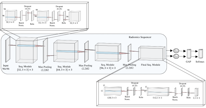
Figure 1: Overview of the proposed deep stacked interpretable sequencing cell (SISC) architecture used as the radiomic sequencer within a discovery radiomics framework. The SISC radiomic sequencer is formed by stacking interpretable sequencing cells together, each comprised of different specialized convolutional layers along with max-pooling and dropout operations. A typical interpretable sequencing cell consists of a block of convolutional layers followed by batchnorm, dropout, and ReLU layers, repeated three times. The final interpretable sequencing cell is flexible and can be changed based on the input and task. Here, the final layer in the last cell consists of two 1$\times$1 convolutions as this study is focused on binary lung cancer classification.

Until recently, state-of-the-art CAD systems relied on radiomics-based approaches built from hand-engineered radiomic features. These features are designed to characterize cancer phenotypes in a high-dimensional feature space that facilitates tumor discrimination. The extracted radiomic sequence consists of a large number of predefined, hand-engineered features for capturing image-based traits such as intensity, texture, and shape. These hand-engineered features can greatly limit the ability of the radiomic sequence to fully characterize the unique traits of different forms of cancer. More recently, the concept of discovery radiomics [4, 5, 6, 7, 8] was shown to achieve state-of-the-art performance. In discovery radiomics, the radiomic sequencers generate highly-discriminative quantitative radiomic features which are discovered, rather than hand-engineered, from vast amounts of available archival medical data. In particular, radiomic sequencers with deep convolutional architectures that are discovered in an end-to-end manner were shown to consistently achieve state-of-the art performance in medical imaging analysis. The use of such radiomic sequencers within the discovery radiomics framework is particularly effective for lung cancer prediction using CT imaging. This is due to the availability of very large annotated CT scan data sets such as LIDC-IDRI [9], which enables highly discriminative radiomic features to be discovered directly from this wealth of data.

Despite the effectiveness of discovery radiomics-based approaches from a diagnostic performance perspective, a key challenge that still remains is the difficulty in interpreting the rationale behind their predictions. As such, one can view such radiomics-based approaches as ’black box’, and the lack of transparency in their decision-making processes makes it difficult for radiologists to verify, validate, and ultimately trust the predictions being made. To enable the widespread adoption of discovery radiomics within CAD systems, one needs to improve radiologists’ trust by providing interpretable reasoning behind the predictions made by radiomic sequencers.

Motivated by this, we propose an end-to-end interpretable discovery radiomics-driven lung cancer prediction pipeline. Specifically, the main contributions of our approach are:

• the introduction of SISC architecture (Fig. 1), comprising of interpretable sequencing cells, for building radiomic sequencers with state-of-the-art performance for lung cancer prediction, and

• interpretable lung cancer predictions in the form of critical response maps generated through a stack of interpretable sequencing cells which highlight the key critical regions leveraged in the prediction process (Fig. 2).

II Background

There has been significant interest and a wealth of literature in the past decade, especially in lung cancer detection and diagnosis [10, 11, 12, 13, 14, 15]. CAD systems designed for automated lung cancer diagnosis can be divided into two main stages: 1) Lung nodule detection and segmentation; and 2) malignancy classification of segmented nodules.

The first stage consists of processing CT images to isolate the lung region [16] and search for potential pulmonary nodule candidates [17, 18]. The process involves finding the location of the pulmonary nodules in a given CT scan slice by defining its position and contour [19]. The candidate detection step is usually followed by false positive reduction algorithms [20, 21, 22] to control the rate of candidate generation.

The second stage is the nodule classification process, where the detected nodules are classified as either malignant or benign. In particular, there has been significant interest in the concept of radiomics, which involves the high-throughput extraction and analysis of a large amount of quantitative features from medical imaging data to characterize tumor phenotypes in a quantitative manner. Different radiomic feature extraction techniques and algorithms have been proposed in the literature to perform the classification task, and can be split into two broad categories: 1) hand-engineered radiomic features, and 2) learned/discovered radiomic features.

II-A Hand-Engineered Radiomic Features

Traditional radiomics-based approaches leveraged pre-defined, hand-engineered features designed with the help of radiologists  [23, 24, 25]. Such hand-engineered features typically capture generic image-based traits such as intensity, texture, and shape. For example, Way et al. [26] used the segmented nodules to extract texture features and classified them using linear discriminant classifier. El-Baz et al. [27] used the shape of nodules as features whereas, Han et al. [28] used 3D texture analysis to extract discriminative features for nodule classification. Dhara et al. [29] used an ensemble of margin-based, shape-based and texture-based features extracted from the segmented nodule to form the feature set. Support vector machines were then used to classify the nodule as malignant or benign using this radiomic feature set.

Aydin et al. [23] used radiologist-provided evaluations to develop a weighted rule-based algorithm using an ensemble of classifiers to predict malignancy score. Recently, Robherson et al. [11] used taxonomic diversity index and mean plylogenetic distance to calculate the malignancy score. In general, the most commonly used feature extraction methods are histogram of oriented gradients (HOG) [30, 31] and local binary patterns (LBP) [32]. Different machine learning classifiers such as support vector machines (SVM) [33], random forests [34] and weighted nearest neighbour (NN) [35] were used with the hand-crafted features for classification. One limitation to hand-engineered radiomic features is that they are typically designed based on generic image-based features that are not customized for the task of lung cancer detection and diagnosis, and thus can greatly limit the classifier’s ability to fully characterize the unique traits of different forms of cancer.

II-B Learned/Discovered Radiomic Features

With the recent advances and success in machine learning, particularly deep learning [36], many researchers have started to leverage such approaches for medical image analysis [37, 38, 39, 40, 4]. This has led to significant interest in the concept of discovery radiomics, where high-dimensional quantitative radiomic features are learned and discovered directly from the wealth of medical imaging data available. Such discovered radiomic sequences enable a much more customized characterization of tumor phenotype. As one of the first deep learning-driven discovery radiomics approaches for the purpose of lung cancer classification, Kumar et al. [41] learned deep radiomic features using an auto-encoder radiomic sequencer for the purpose of classifying lung nodules as malignant or benign. Currently, deep convolutional radiomic sequencers have shown tremendous success for the task of nodule classification. With sufficient architectural depth, these radiomic sequencers enable a robust classification framework that can accommodate the variability found in characteristics of the lung nodules. For example, Mario et al. [24] combined shape and appearance radiomic features with learnt radiomic features from a deep convolutional radiomic sequencer to form a combined radiomic sequence that is then used to feed a random forest classifier. Shen et al. [42] proposed a multi-scale convolutional radiomic sequencer to obtain radiomic features for the purpose of nodule classification. Zhao et al. [37] proposed a hybrid radiomic sequencer to combine deep convolutional features with LBP and HOG features. A novel multi–scale, multi–view radiomic sequencer architecture was proposed by Liu et al. [14] for nodule classification. The 3D nature of the CT scans has also inspired the use of 3D convolutional radiomic sequencer architectures. Liu et al. [43] proposed a novel 3D convolutional architecture for lung nodule classification. Zhu et al. [44] proposed an end–to–end automated lung cancer detection framework called ”DeepLung”, where 3D dual path net feature extraction was introduced. Dey et al. [45] proposed a two-pathway 3D convolutional architecture to capture both local and global characteristics.

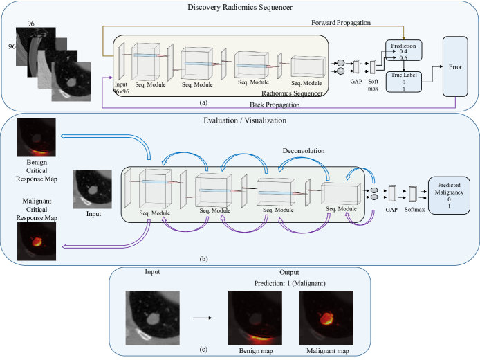
Figure 2: Overview of the end-to-end interpretable discovery radiomics-driven framework for lung cancer prediction. Part (a) shows the sequencer discovery process, where a specialized radiomic sequencer, comprised of a deep stack of interpretable sequencer cells, is discovered for the given set of CT lung nodule data. Part (b) presents the cancer prediction process, where the discovered radiomic sequencer is used to make a prediction based on CT data and how interpretable critical response maps are generated through the stack of sequencer cells. In part (b), the input CT data of a new patient is fed into the radiomic sequencer to generate a radiomic sequence and perform prediction on whether it is a benign and malignant case. To generate the critical response map, the output of the last layer in the sequencing cell of the radiomic sequencer is backpropagated through each sequencing cell using the method described in Section III-C for each of the possible prediction states (benign and malignant). As such, we obtained two critical response maps, each highlighting the critical regions used by the sequencer for making predictions regarding whether the given input nodule is benign or malignant. The last part (c) is the interface seen by the end user, which shows the given input, the prediction and evidence been used to obtain the particular prediction through critical response map.

II-C Interpretability

While highly complex deep convolutional radiomic sequencer architectures can achieve state-of-the-art performance, one of the biggest limitations to leveraging such sequencers is that they are very difficult to interpret. As such, researchers have in recent years explored different approaches for better understanding the inner workings of such architectures. The current approaches can be grouped into two categories. The first group of approaches attempts to understand the global decision making process of the deep convolutional architectures by identifying inputs which maximize the outputs in the architecture [46, 47, 48, 49]. The second group of approaches provides an explanation for the prediction being made by generating attentive maps for the input image. The attentive maps highlight the attentive regions used by the architecture for making a particular prediction. Since it is important for clinicians interacting with a CAD system to be able to visualize critical regions linked to cancer and for the purpose of justifying the computer-aided lung cancer prediction, we will discuss the second group of approaches in detail below.

Simonyan et al. [50] used derivatives of the class score found by back-propagation for each pixel to create the class saliency map. Zeiler et al. [51] and Springenberg et al. [52] used a deconvolution-based method and gradient-based method, respectively, to project activations back to the input space. A limitation of both methods is that there is no class information to their visualizations. Zhou et al. [53] proposed to use global average pooling layers in CNN to create what they refer to as Class Activation Maps (CAM). Zintgraf et al. [54] proposed to use multi-variate conditional sampling to visualize the predictions made by deep convolutional architectures and highlight the input image’s pixel which contributes for and against a particular class. Kumar et al. [55] proposed the concept of CLEAR (CLass-Enhanced Attentive Response) maps which can provide the per-class attentive interest levels on each input image’s pixel in the given deep convolutional architecture.

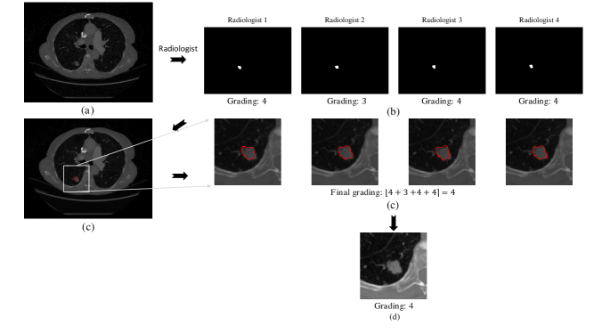
Figure 3: Data preparation flow for i) computing malignancy score, and ii) obtaining an 96$\times$96 nodule image directly from the raw LIDC-IDRI dataset. For a given lung CT slice image (a), the LIDC-IDRI dataset contains lung nodule masks from up to four radiologist (b). We use these masks to locate the contour of the nodule in the CT slice image. As can be seen in the zoomed-in images in (c), the contours of the mask differ due to the inter-observer variability. To mitigate this, we selected an sub-image of 96$\times$96 from the average center pixel obtained from the radiologist masks to create a single 96$\times$96 lung nodule image (d). For computing the malignancy score (as shown in (d)), we average the scores given by the radiologists as indicated in part (c). A detailed discussion on data preparation is discussed in Section III part A.

III Methodology

This section describes the design and implementation of a radiomics sequencer. The modular design of the SISC architecture (see Section III-B) enables a significant reduction in the design search space while improving classification performance. Furthermore, the introduction of interpretable sequencing cells allow us to achieve end-to-end interpretability through the generation of critical region maps to aid the clinician in the decision-making process (see Section III-C). The LIDC-IDRI dataset (see Section III-A) is used to validate the proposed radiomic sequencer architecture.

III-A Dataset

The Lung Image Database Consortium (LIDC) and Image Database Resource Initiative (IDRI) [9] published a structured and categorized repository of computed tomography (CT) scans to assist the development of CAD methods for automated lung cancer diagnosis. The dataset consists of 1018 thoracic CT scans, where each scan is processed by four radiologists at both blinded and un–blinded stages. In the blinded stage, each radiologist reviews the CT scans without inputs from other radiologists. In the second, un–blinded stage, each radiologist is shown the results of other radiologists from the blinded stage and is given a chance to change their initial evaluations. The two stage process was designed to provide the best estimate of the nodule characteristics.

The suspected lung lesions in the LIDC dataset are divided into three categories: i) Non-nodule$\geq$3mm, ii) Nodule$\geq$3mm, and iii) Nodule$<$3mm, where the diameter is measured as the length of the lesion’s longest axis. For each category, different nodule characteristics are included in the dataset. Similar to previous methods, we decided to only use Nodule$\geq$3mm. For the Nodule$\geq$3mm category, the required malignancy score along with the nodule location and contour information by at least one radiologist are included. Therefore, the Nodule$\geq$3mm category is used for our experiments. A total of $2669$ nodules are reported in the dataset under the Nodule$\geq$3mm category.

For each nodule, its characteristics are provided by at most four radiologists. The final malignancy score for each nodule is obtained by combining the scores from all of the radiologists. As suggested in [28], the average score rounded to the nearest integer was taken as the final malignancy score. In each slice of the given nodule, a $96\times 96$ window was cropped at the nodule center. The size was determined to accommodate for all the variability in the nodule contour and also to include sufficient background information. The same malignancy score was assigned for all the slices in the given nodule. A total of $14,433$ nodule images along with their corresponding malignancy score were extracted from the dataset.

III-B Interpretable Sequencing Cells

A modular design strategy was leveraged to construct the proposed SISC radiomics sequencer, where the underlying architecture is comprised of a deep stack of interpretable sequencing cells with similar micro-architectures. More specifically, an intepretable sequencing cell as introduced in this study comprises of a block of convolutional layers along with max-pooling and dropout operations, all optimized using the available data. The proposed SISC radiomic sequencer is then constructed by stacking the interpretable sequencing cells together in a depth-wise manner. The aim is to reduce the design search space while improving classification accuracy, thus enabling optimized design of sequencer architectures in a more predictable manner. The micro-architecture of an interpretable sequencing cell is defined by three convolutional layers separated by batch normalization [56] and drop–out [57]. Furthermore, the ReLU [58] activation is used after each convolutional layer. The interpretable sequencing cell is optimized by sharing the same architectural values. For example, all the dropout layers in a given interpretable sequencing cell have the same dropout rate.

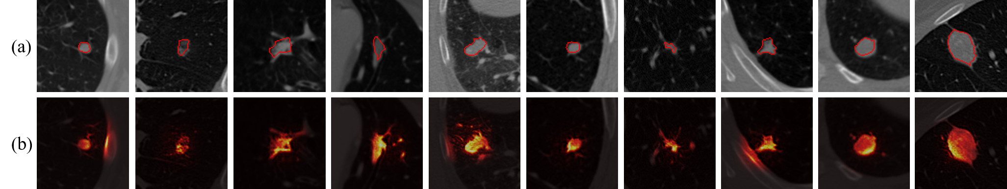
Figure 4: Example critical response maps for malignant cases. (a) original 96$\times$96 malignant nodule sub-image taken from lung CT slices with the radiologist-provided best contours for a given patient CT slice image, and (b) corresponding critical response maps showing the malignant critical regions been used for correctly predicting malignant nodules. It can be seen that for almost all the example cases, the proposed SISC radiomic sequencer uses clinically relevant markers when achieving correct predictions. Therefore, the use of critical response maps can potentially improve the overall confidence of the clinician on the discovered SISC radiomic sequencer.

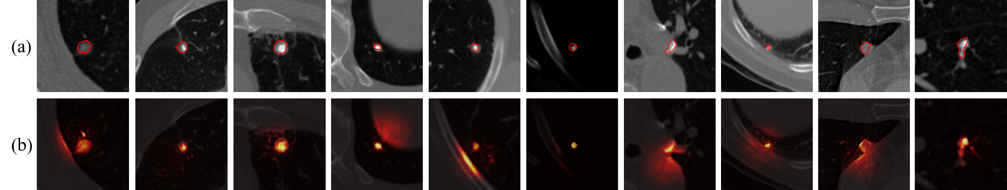
Figure 5: Example critical response maps for benign cases. (a) original 96$\times$96 malignant nodule sub-image taken from lung CT slices with the radiologist-provided best contours for a given patient CT slice image, and (b) corresponding critical response maps showing the benign critical regions been used for correctly predicting benign nodules. It can be seen that for almost all the example cases, the proposed SISC radiomic sequencer uses clinically relevant markers when achieving correct predictions. Therefore, as with the previous figure, the use of critical response maps can potentially improve the overall confidence of the clinician on the discovered SISC radiomic sequencer.

In this study, the proposed SISC radiomic sequencer is comprised of four interpretable sequencing cells stacked together in a depth-wise manner as shown in Fig 1. The number of channels is increased as we go deeper into the SISC architecture whereas the size of the kernel is fixed for the first three cells. Each cell is followed by a max pooling layer. The dropout, batch normalization parameters and number of cells are optimized with the LIDC-IDRC dataset. The final cell of the SISC radiomic sequencer is defined as shown in Fig. 1. The number of kernels in the final convolutional layer of the final cell is equivalent to the total number of classes to enable end-to-end interpretability via critical response maps, which will be further discussed in the following section. The final convolutional layer is followed by a global average pooling layer, which is then followed by a softmax output layer.

The proposed SISC radiomic sequencer formed by the stacking of interpretable sequencing cells with learned parameters is shown in Fig 1. We can observe that the repeated modular approach allows us to compactly define the sequencer with a minimum number of configurable architectural parameters. The modular approach also leads to state-of-the-art results as described in Section IV.

III-C Interpretability through Critical Response Maps

To enable interpretability and explainability in the decision-making process of the proposed SISC radiomic sequencer, we take inspiration from [55] and [59] and introduce an approach where critical response maps are generated through the entire stack of interpretable sequencing cells. An critical response map provides spatial insights on critical regions in the CT scan and their level of contribution to a particular prediction made. Here, an individual critical response map is generated for each possible prediction (benign and malignant).

Using these critical response maps, the clinician can not only validate the the evidence behind the predictions made using the proposed SISC radiomic sequencer, but the maps also help in locating relevant regions in the CT scan responsible for either a malignant or benign nodule prediction. An example pair of critical response maps can be seen in Fig. 2.

For example, in the case of a malignant nodule, a successful and reasonable prediction should lead to the malignant critical map highlighting the nodule regions. As such, critical response maps may potentially help radiologists to have greater confidence in the CAD system and in aiding them with their clinical diagnosis decisions.

The critical response map generation process can be described as follows. Let the critical response maps $A(x|c)$ for a given CT scan slice image $x$ for each prediction $c$ be computed via back-propagation from the last layer of the last interpretable sequencing cell in the proposed SISC radiomic sequencer. The notation used in this study are based on the study done by Kumar et. al.[55] for consistency. As shown in Fig 1, the last layer in the interpretable sequencing cell at the end of the proposed SISC radiomic sequencer contains $N=2$ nodes, equal to the number of possible predictions (i.e., benign and malignant). The output activations of this layer are followed by global average pooling and then a softmax output layer. So, to create the critical maps for each possible prediction, the back-propagation starts with the individual prediction nodes in the last layer to the input space. For a single layer $l$, The deconvolved output response $\hat{r}_{l}$ is given by,

$$\hat{h}_{l}=\sum_{k=1}^{K}f_{k,l}*p_{k,l}$$ (1)

where $f_{k}$ is the feature map and $p_{l}$ is the kernel of layer $l$. the symbol $*$ represents the convolution operator. For simplicity, The convolution and summation can be combined as $\hat{h}_{l}=D_{l}f_{l}$. Therefore, the critical response map $A(\stackunder[1.2pt]{$x$}{\rule{3.44444pt}{0.32289pt}}|c)$, for a given prediction $c$ is defined as,

$$A(\stackunder[1.2pt]{x}{\rule{3.44444pt}{0.32289pt}}|c)=D_{1}M^{\prime}_{1}D_{2}M^{\prime}_{2}....D_{L-1}M^{\prime}_{L-1}D^{c}_{L}F_{L}.$$ (2)

Where $M^{\prime}$ is the un-pooling operation as described in [60] and $D^{c}_{L}$ is the convolution operation at the last layer with kernel $p_{L}$ replaced by zero except at the $c^{th}$ location corresponding to the prediction $c$.

IV Experiments and Results

In this section, we will evaluate and discuss the efficacy for the proposed SICS radiomic sequencer for the purpose of lung cancer prediction on two main fronts: i) cancer prediction performance of the proposed sequencer compared to state-of-the-art, and ii) interpretability of the cancer predictions made by the proposed sequencer through the generated critical response maps.

IV-A Experimental Setup

TABLE I: Number of samples for corresponding malignancy scores, for three different datasets. The datasets were created based on how the radiologist malignancy rating 3 was treated i.e., Ignored (I), treated as benign (B), or treated as malignant (M).

Malignancy score	Size	I	B	M
1	1376	3981	9638	3981
2	2605
3	5657	Ignored		10452
4	3192	4795	4795
5	1603

The setup of the experiments in this study can be described as follows. The cropped lung nodule images with their corresponding malignancy scores are obtained from the LIDC-IDRI dataset as explained in section III-A. The distribution of the malignancy scores in the dataset is described in Table I. Malignancy scores $1$ and $2$ are considered as benign, whereas scores $4$ and $5$ are considered as Malignant. The malignancy score $3$ can be either considered as benign, malignant or ignored depending as done by previous studies in this field. In this paper, we have created three different datasets where the score $3$ is considered malignant (dataset: ‘M’), benign (dataset: ‘B’), and ignored (Dataset: ‘I’). The final dataset distribution is shown in Table I. Each dataset was further divided into $80\%$ training data, $10\%$ for validation and $10\%$ testing data. The pre-processing and dataset distribution is similar to Xie et. al. [10].

Table II shows the distribution of training data for the three datasets. We can observe that dataset ‘B’ and ‘M’ are not evenly distributed. To mitigate this imbalance, data augmentation was performed on each of the datasets to balance the number of examples associated with each class. Furthermore, the data augmentation performed also acts to enhance the variability and generalizability of the radiomic sequencer. In particular, random horizontal shifts, vertical shifts, and rotations were applied along with vertical and horizontal flips to construct the augmented training dataset. Since the size of the training data has a huge impact on the performance of the proposed radiomic sequencer, three different augmented datasets with varying size were created for each of the ‘M’, ‘B’ and ‘I’ datasets, as shown in Table II. The performance of dataset ’I’ under different levels of data augmentation is shown in Fig 10. We can observe that the $\approx 15$k size yielded the best performance. Going forward, we have finalized the dataset size to be $\approx 15$k for further hyper-parameter tuning and validations for the ‘M’, ‘B’ and ‘I’ datasets.

Different data normalization techniques such as standard deviation, Min-Max, and ZCA whitening [61] were also applied to the lung nodule images. It was found that Min-Max normalization yielded the best results. After optimizing the hyper-parameter using the validation set, batch normalization was implemented with momentum$=0.99$ and dropout layer was used with rate$=0.25$. The Adam optimizer was used with learning rate $=1e^{-}5$ and batch size as $128$. The proposed radiomic sequencer was learnt for approximately $200$ epochs and evaluated against the test dataset. The final results were reported by averaging over 10-fold cross validation for all three datasets.

IV-B Cancer prediction performance

To evaluate the cancer prediction performance of the proposed SISC radiomic sequencer, we computed the sensitivity, specificity, accuracy, and AUC of the proposed sequencer and compared it with five other state-of-the-art approaches. The average lung cancer prediction performance of the proposed radiomic sequencer for dataset ‘M’, ‘B’ and ‘I’ are shown in Table. V & IV & III respectively. The AUC curves of the 10 different cross validation runs for each dataset are shown in Figs. 6, 7 & 8. The best performing AUC curve from each dataset is shown in Fig. 9. From the results, we can observe that, for the dataset ‘I’, by leveraging the proposed SISC radiomic sequencer, we were able to achieve comparable performance with the current state-of-the-art method proposed by Xie et al. [10]. For datasets ‘B’ and ‘M’, the proposed sequencer is able to outperform the accuracy results from Xie et al. [10]. The comparison of the existing and current state-of-the-art methods with the proposed SISC radiomic sequencer is given in Table. V & IV & III. The comparison methods are based on the previous studies in this field, employing the same data pre–processing steps for fair comparison amongst the methods. Based on these experimental results, it can be observed that the proposed SISC radiomic sequencer can provide strong cancer prediction performance that exceeds state-of-the-art in all but one case, where in that case the performance is comparable to state-of-the-art.

TABLE II: Dataset distribution for the three different dataset configuration obtained from the LIDC-IDRI dataset before and after data augmentation (as described in Section IV-A).

Dataset	Grade	Before Data Aug	15k	30k	60k
I	Malignant	3836	9836	15836	30836
	Benign	3184	9184	15184	30184
	Total	7020	19020	31020	61020
B	Malignant	3836	7672	19180	38360
	Benign	7712	7712	21712	35712
	Total	11548	15384	40892	74072
M	Malignant	8361	8361	16361	33444
	Benign	3187	6374	15935	28683
	Total	11548	14735	32296	62127

TABLE III: Performance comparison between tested cancer prediction methods for the ignored (I) dataset. Best results are highlighted in bold.

Method	Accuracy	Sensitivity	Specificity	AUC
Han et al. [28]	85.59	70.62	93.02	89.25
Dhara et al. [29]	88.38	84.58	90.03	95.76
Shen et al. [38]	87.14	77.00	93.00	93.00
Sun et al. [62]	-	-	-	88.23$\pm$1.70
Xie et al. [10]	89.53$\pm$0.09	84.19$\pm$0.09	92.02$\pm$0.01	96.65$\pm$0.01
Ours (SISC)	89.36$\pm$1.20	90.28$\pm$2.00	88.25$\pm$2.00	96.01$\pm$0.70

TABLE IV: Performance comparison between tested cancer prediction methods for the benign (B) dataset. Best results are highlighted in bold.

Method	Accuracy	Sensitivity	Specificity	AUC
Han et al. [28]	87.36	73.75	93.37	93.79
Dhara et al. [29]	87.69	80.00	89.30	94.44
Xie et al. [10]	87.74$\pm$0.03	81.11$\pm$0.85	89.67$\pm$0.09	94.45$\pm$0.01
Ours (SISC)	88.57$\pm$1.70	78.32$\pm$8.12	93.66$\pm$2.06	94.34$\pm$0.08

TABLE V: Performance comparison between tested cancer prediction methods for the malignant (M) dataset. Best results are highlighted in bold.

Method	Accuracy	Sensitivity	Specificity	AUC
Kumar et al. [41]	75.01	83.35	-	-
Han et al. [28]	70.97	53.61	89.41	76.26
Dhara et al. [29]	71.17	53.47	89.74	79.74
Sharma et al. [63]	84.13	91.69	73.16	-
Xie et al. [10]	71.93$\pm$0.04	59.22$\pm$0.04	84.85$\pm$0.10	81.24$\pm$0.01
Ours (SISC)	84.17$\pm$1.50	90.71$\pm$4.01	67.00$\pm$8.64	89.06$\pm$1.20

Res

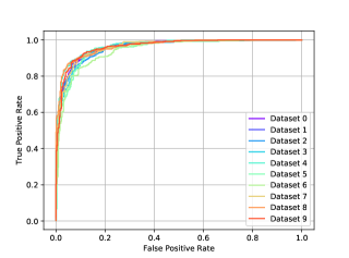
Figure 6: Receiver operating curve (ROC) for the ignored (I) dataset for 10 different cross validation runs.

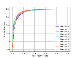
Figure 7: Receiver operating curve (ROC) for the benign (B) dataset for 10 different cross validation runs.

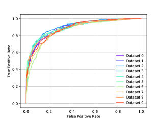
Figure 8: Receiver operating curve (ROC) for the malignant (M) dataset for 10 different cross validation runs.

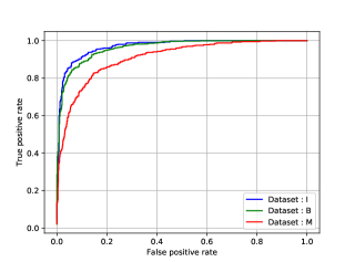
Figure 9: Comparing the best ROC curves for the three different datasets: ignored (I), benign (B) and malignant (M).

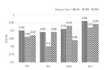
Figure 10: Accuracy, sensitivity, and specificity for the “ignored” (I) dataset for three different training sample sizes. It can be observed that the $\approx$15k size performed the best for 3 out of 4 metrics, including AUC; hence it was chosen as the default training size for the three different dataset categories: ignored (I), benign (B), and malignant (M).

IV-C Interpretability

Here, we will investigate the efficacy of the proposed SISC radiomic sequencer in terms of interpretability of the lung cancer predictions made. Fig. 4 shows example critical response maps generated in an end-to-end manner for several example malignant nodule images that were correctly predicted to be malignant. From the figure, it can be observed that the proposed SISC radiomic sequencer is able to successfully identify the nodule regions in the given CT slices without being explicitly directed to do so. As shown in Fig. 4, the highlighted region’s contour closely matches the contours given by the radiologists, and in some cases provide improved contour localization than that provided by the radiologists. The proposed SISC radiomic sequencer is able to successfully highlight a wide range of nodules with different shapes and sizes. We can also infer the discriminative nature of the proposed sequencer by observing that the highlighted regions in the critical response maps that contribute highly to a malignancy prediction. This helps to gain better insight in the rationale behind the malignancy prediction. Similar observations can also be observed for benign nodules as shown in Fig.5.

Due to the end-to-end interpretable nature of the proposed SISC radiomic sequencer, the critical response maps produced through the entire stack of interpretable sequencing cells can potentially help improve the confidence of radiologists working with the CAD system. Furthermore, the critical response maps can also assist radiologists to more consistently and rapidly spot abnormal nodules within the large volume of a CT scan, as well as understand the nature and characteristics most linked to malignancy.

V Conclusion

In this paper, we introduce a novel end-to-end interpretable discovery radiomics-driven lung cancer prediction framework. This framework is enabled by the proposed radiomic sequencer: a deep stacked interpretable sequencing cell (SISC) architecture comprised of interpretable sequencing cells. Experimental results show that the proposed SISC radiomic sequencer is able to not only achieve state-of-the-art results in lung cancer prediction, but also offers prediction interpretability in the form of critical response maps generated through the stack of interpretable sequencing cells which highlights the critical regions used by the sequencer for making predictions. The critical response maps are useful for not only validating the predictions of the proposed SISC radiomic sequencer, but also provide improved radiologist-machine collaboration for improved diagnosis.

References

- [1] H. Nagai and Y. H. Kim, “Cancer prevention from the perspective of global cancer burden patterns,” in Journal of thoracic disease, vol. 9, no. 3. AME Publications, 2017, p. 448.
- [2] C. for Disease Control and . c. s. Prevention, “https://www.cdc.gov/cancer/lung/statistics/,” 2016.
- [3] M. Zanon, G. S. Pacini, V. V. S. de Souza, E. Marchiori, G. S. P. Meirelles, G. Szarf, F. S. Torres, and B. Hochhegger, “Early detection of lung cancer using ultra-low-dose computed tomography in coronary ct angiography scans among patients with suspected coronary heart disease,” in Lung Cancer, vol. 114. Elsevier, 2017, pp. 1–5.
- [4] A. G. Chung, M. J. Shafiee, D. Kumar, F. Khalvati, M. A. Haider, and A. Wong, “Discovery radiomics for multi-parametric mri prostate cancer detection,” in arXiv preprint arXiv:1509.00111, 2015.
- [5] M. J. Shafiee, A. G. Chung, D. Kumar, F. Khalvati, M. Haider, and A. Wong, “Discovery radiomics via stochasticnet sequencers for cancer detection,” in arXiv preprint arXiv:1511.03361, 2015.
- [6] D. Kumar, A. G. Chung, M. J. Shaifee, F. Khalvati, M. A. Haider, and A. Wong, “Discovery radiomics for pathologically-proven computed tomography lung cancer prediction,” in International Conference Image Analysis and Recognition. Springer, 2017, pp. 54–62.
- [7] A. Wong, A. G. Chung, D. Kumar, M. J. Shafiee, F. Khalvati, and M. Haider, “Discovery radiomics for imaging-driven quantitative personalized cancer decision support,” in Journal of Computational Vision and Imaging Systems, vol. 1, no. 1, 2015.
- [8] A.-H. Karimi, A. G. Chung, M. J. Shafiee, F. Khalvati, M. A. Haider, A. Ghodsi, and A. Wong, “Discovery radiomics via a mixture of deep convnet sequencers for multi-parametric mri prostate cancer classification,” in International Conference Image Analysis and Recognition. Springer, 2017, pp. 45–53.
- [9] S. G. Armato, G. McLennan, L. Bidaut, M. F. McNitt-Gray, C. R. Meyer, A. P. Reeves, B. Zhao, D. R. Aberle, C. I. Henschke, E. A. Hoffman et al., “The lung image database consortium (lidc) and image database resource initiative (idri): a completed reference database of lung nodules on ct scans,” in Medical physics, vol. 38, no. 2. Wiley Online Library, 2011, pp. 915–931.
- [10] Y. Xie, J. Zhang, Y. Xia, M. Fulham, and Y. Zhang, “Fusing texture, shape and deep model-learned information at decision level for automated classification of lung nodules on chest ct,” in Information Fusion, vol. 42. Elsevier, 2018, pp. 102–110.
- [11] A. O. de Carvalho Filho, A. C. Silva, A. C. de Paiva, R. A. Nunes, and M. Gattass, “Classification of patterns of benignity and malignancy based on ct using topology-based phylogenetic diversity index and convolutional neural network,” in Pattern Recognition, vol. 81. Elsevier, 2018, pp. 200–212.
- [12] W. Zhu, C. Liu, W. Fan, and X. Xie, “Deeplung: Deep 3d dual path nets for automated pulmonary nodule detection and classification,” in arXiv preprint arXiv:1801.09555, 2018.
- [13] S. Shen, S. X. Han, D. R. Aberle, A. A. Bui, and W. Hsu, “An interpretable deep hierarchical semantic convolutional neural network for lung nodule malignancy classification,” in arXiv preprint arXiv:1806.00712, 2018.
- [14] X. Liu, F. Hou, H. Qin, and A. Hao, “Multi-view multi-scale cnns for lung nodule type classification from ct images,” in Pattern Recognition. Elsevier, 2018.
- [15] Z. Wang, J. Xin, P. Sun, Z. Lin, Y. Yao, and X. Gao, “Improved lung nodule diagnosis accuracy using lung ct images with uncertain class,” in Computer methods and programs in biomedicine, vol. 162. Elsevier, 2018, pp. 197–209.
- [16] S. Shen, A. A. Bui, J. Cong, and W. Hsu, “An automated lung segmentation approach using bidirectional chain codes to improve nodule detection accuracy,” in Computers in biology and medicine, vol. 57. Elsevier, 2015, pp. 139–149.
- [17] K. Suzuki, “A supervised ‘lesion-enhancement’filter by use of a massive-training artificial neural network (mtann) in computer-aided diagnosis (cad),” in Physics in Medicine & Biology, vol. 54, no. 18. IOP Publishing, 2009, p. S31.
- [18] N. Duggan, E. Bae, S. Shen, W. Hsu, A. Bui, E. Jones, M. Glavin, and L. Vese, “A technique for lung nodule candidate detection in ct using global minimization methods,” in International Workshop on Energy Minimization Methods in Computer Vision and Pattern Recognition. Springer, 2015, pp. 478–491.
- [19] O. Ronneberger, P. Fischer, and T. Brox, “U-net: Convolutional networks for biomedical image segmentation,” in International Conference on Medical image computing and computer-assisted intervention. Springer, 2015, pp. 234–241.
- [20] K. Suzuki, S. G. Armato, F. Li, S. Sone et al., “Massive training artificial neural network (mtann) for reduction of false positives in computerized detection of lung nodules in low-dose computed tomography,” in Medical physics, vol. 30, no. 7. Wiley Online Library, 2003, pp. 1602–1617.
- [21] K. Suzuki, J. Shiraishi, H. Abe, H. MacMahon, and K. Doi, “False-positive reduction in computer-aided diagnostic scheme for detecting nodules in chest radiographs by means of massive training artificial neural network1,” in Academic Radiology, vol. 12, no. 2. Elsevier, 2005, pp. 191–201.
- [22] K. Suzuki, S. G. Armato, F. Li, S. Sone, and K. Doi, “Effect of a small number of training cases on the performance of massive training artificial neural network (mtann) for reduction of false positives in computerized detection of lung nodules in low-dose ct,” in Medical Imaging 2003: Image Processing, vol. 5032. International Society for Optics and Photonics, 2003, pp. 1355–1367.
- [23] A. Kaya and A. B. Can, “A weighted rule based method for predicting malignancy of pulmonary nodules by nodule characteristics,” in Journal of biomedical informatics, vol. 56. Elsevier, 2015, pp. 69–79.
- [24] M. Buty, Z. Xu, M. Gao, U. Bagci, A. Wu, and D. J. Mollura, “Characterization of lung nodule malignancy using hybrid shape and appearance features,” in International Conference on Medical Image Computing and Computer-Assisted Intervention. Springer, 2016, pp. 662–670.
- [25] P. Huang, S. Park, R. Yan, J. Lee, L. C. Chu, C. T. Lin, A. Hussien, J. Rathmell, B. Thomas, C. Chen et al., “Added value of computer-aided ct image features for early lung cancer diagnosis with small pulmonary nodules: A matched case-control study,” in Radiology, vol. 286, no. 1. Radiological Society of North America, 2017, pp. 286–295.
- [26] T. W. Way, L. M. Hadjiiski, B. Sahiner, H.-P. Chan, P. N. Cascade, E. A. Kazerooni, N. Bogot, and C. Zhou, “Computer-aided diagnosis of pulmonary nodules on ct scans: Segmentation and classification using 3d active contours,” in Medical physics, vol. 33, no. 7Part1. Wiley Online Library, 2006, pp. 2323–2337.
- [27] A. El-Baz, M. Nitzken, F. Khalifa, A. Elnakib, G. Gimel’farb, R. Falk, and M. A. El-Ghar, “3d shape analysis for early diagnosis of malignant lung nodules,” in Biennial International Conference on Information Processing in Medical Imaging. Springer, 2011, pp. 772–783.
- [28] F. Han, G. Zhang, H. Wang, B. Song, H. Lu, D. Zhao, H. Zhao, and Z. Liang, “A texture feature analysis for diagnosis of pulmonary nodules using lidc-idri database,” in Medical Imaging Physics and Engineering (ICMIPE), 2013 IEEE International Conference on. IEEE, 2013, pp. 14–18.
- [29] A. K. Dhara, S. Mukhopadhyay, A. Dutta, M. Garg, and N. Khandelwal, “A combination of shape and texture features for classification of pulmonary nodules in lung ct images,” in Journal of digital imaging, vol. 29, no. 4. Springer, 2016, pp. 466–475.
- [30] N. Dalal and B. Triggs, “Histograms of oriented gradients for human detection,” in Computer Vision and Pattern Recognition, 2005. CVPR 2005. IEEE Computer Society Conference on, vol. 1. IEEE, 2005, pp. 886–893.
- [31] M. Firmino, G. Angelo, H. Morais, M. R. Dantas, and R. Valentim, “Computer-aided detection (cade) and diagnosis (cadx) system for lung cancer with likelihood of malignancy,” in Biomedical engineering online, vol. 15, no. 1. BioMed Central, 2016, p. 2.
- [32] T. Ojala, M. Pietikainen, and T. Maenpaa, “Multiresolution gray-scale and rotation invariant texture classification with local binary patterns,” in IEEE Transactions on pattern analysis and machine intelligence, vol. 24, no. 7. IEEE, 2002, pp. 971–987.
- [33] F. Han, H. Wang, G. Zhang, H. Han, B. Song, L. Li, W. Moore, H. Lu, H. Zhao, and Z. Liang, “Texture feature analysis for computer-aided diagnosis on pulmonary nodules,” in Journal of digital imaging, vol. 28, no. 1. Springer, 2015, pp. 99–115.
- [34] S. G. Armato, K. Drukker, F. Li, L. Hadjiiski, G. D. Tourassi, J. S. Kirby, L. P. Clarke, R. M. Engelmann, M. L. Giger, G. Redmond et al., “Lungx challenge for computerized lung nodule classification,” in Journal of Medical Imaging, vol. 3, no. 4. International Society for Optics and Photonics, 2016, p. 044506.
- [35] A. P. Reeves, Y. Xie, and A. Jirapatnakul, “Automated pulmonary nodule ct image characterization in lung cancer screening,” in International journal of computer assisted radiology and surgery, vol. 11, no. 1. Springer, 2016, pp. 73–88.
- [36] A. Krizhevsky, I. Sutskever, and G. E. Hinton, “Imagenet classification with deep convolutional neural networks,” in Advances in neural information processing systems, 2012, pp. 1097–1105.
- [37] T. Zhao, H. Wang, L. Li, Y. Qi, H. Gao, F. Han, Z. Liang, Y. Qi, and Y. Cao, “A hybrid cnn feature model for pulmonary nodule differentiation task,” in Imaging for Patient-Customized Simulations and Systems for Point-of-Care Ultrasound. Springer, 2017, pp. 19–26.
- [38] W. Shen, M. Zhou, F. Yang, C. Yang, and J. Tian, “Multi-scale convolutional neural networks for lung nodule classification,” in International Conference on Information Processing in Medical Imaging. Springer, 2015, pp. 588–599.
- [39] W. Li, P. Cao, D. Zhao, and J. Wang, “Pulmonary nodule classification with deep convolutional neural networks on computed tomography images,” in Computational and mathematical methods in medicine, vol. 2016. Hindawi, 2016.
- [40] A. A. A. Setio, F. Ciompi, G. Litjens, P. Gerke, C. Jacobs, S. J. van Riel, M. M. W. Wille, M. Naqibullah, C. I. Sánchez, and B. van Ginneken, “Pulmonary nodule detection in ct images: false positive reduction using multi-view convolutional networks,” in IEEE transactions on medical imaging, vol. 35, no. 5. IEEE, 2016, pp. 1160–1169.
- [41] D. Kumar, A. Wong, and D. A. Clausi, “Lung nodule classification using deep features in ct images,” in Computer and Robot Vision (CRV), 2015 12th Conference on. IEEE, 2015, pp. 133–138.
- [42] W. Shen, M. Zhou, F. Yang, D. Yu, D. Dong, C. Yang, Y. Zang, and J. Tian, “Multi-crop convolutional neural networks for lung nodule malignancy suspiciousness classification,” in Pattern Recognition, vol. 61. Elsevier, 2017, pp. 663–673.
- [43] S. Liu, Y. Xie, A. Jirapatnakul, and A. P. Reeves, “Pulmonary nodule classification in lung cancer screening with three-dimensional convolutional neural networks,” in Journal of Medical Imaging, vol. 4, no. 4. International Society for Optics and Photonics, 2017, p. 041308.
- [44] W. Zhu, C. Liu, W. Fan, and X. Xie, “Deeplung: 3d deep convolutional nets for automated pulmonary nodule detection and classification,” in arXiv preprint arXiv:1709.05538, 2017.
- [45] R. Dey, Z. Lu, and Y. Hong, “Diagnostic classification of lung nodules using 3d neural networks,” in Biomedical Imaging (ISBI 2018), 2018 IEEE 15th International Symposium on. IEEE, 2018, pp. 774–778.
- [46] D. Erhan, A. Courville, and Y. Bengio, “Understanding representations learned in deep architectures,” in Department d’Informatique et Recherche Operationnelle, University of Montreal, QC, Canada, Tech. Rep, vol. 1355, 2010.
- [47] D. Baehrens, T. Schroeter, S. Harmeling, M. Kawanabe, K. Hansen, and K.-R. MÞller, “How to explain individual classification decisions,” in Journal of Machine Learning Research, vol. 11, no. Jun, 2010, pp. 1803–1831.
- [48] I. Goodfellow, H. Lee, Q. V. Le, A. Saxe, and A. Y. Ng, “Measuring invariances in deep networks,” in Advances in neural information processing systems, 2009, pp. 646–654.
- [49] J. Yosinski, J. Clune, A. Nguyen, T. Fuchs, and H. Lipson, “Understanding neural networks through deep visualization,” in arXiv preprint arXiv:1506.06579, 2015.
- [50] K. Simonyan, A. Vedaldi, and A. Zisserman, “Deep inside convolutional networks: Visualising image classification models and saliency maps,” in arXiv preprint arXiv:1312.6034, 2013.
- [51] M. D. Zeiler and R. Fergus, “Visualizing and understanding convolutional networks,” in European conference on computer vision. Springer, 2014, pp. 818–833.
- [52] J. T. Springenberg, A. Dosovitskiy, T. Brox, and M. Riedmiller, “Striving for simplicity: The all convolutional net,” in arXiv preprint arXiv:1412.6806, 2014.
- [53] B. Zhou, A. Khosla, A. Lapedriza, A. Oliva, and A. Torralba, “Learning deep features for discriminative localization,” in Proceedings of the IEEE Conference on Computer Vision and Pattern Recognition, 2016, pp. 2921–2929.
- [54] L. M. Zintgraf, T. S. Cohen, T. Adel, and M. Welling, “Visualizing deep neural network decisions: Prediction difference analysis,” in arXiv preprint arXiv:1702.04595, 2017.
- [55] D. Kumar, A. Wong, and G. W. Taylor, “Explaining the unexplained: A class-enhanced attentive response (clear) approach to understanding deep neural networks,” in IEEE Computer Vision and Pattern Recognition (CVPR) Workshop, 2017.
- [56] S. Ioffe and C. Szegedy, “Batch normalization: Accelerating deep network training by reducing internal covariate shift,” in arXiv preprint arXiv:1502.03167, 2015.
- [57] N. Srivastava, G. Hinton, A. Krizhevsky, I. Sutskever, and R. Salakhutdinov, “Dropout: A simple way to prevent neural networks from overfitting,” in The Journal of Machine Learning Research, vol. 15, no. 1. JMLR. org, 2014, pp. 1929–1958.
- [58] X. Glorot, A. Bordes, and Y. Bengio, “Deep sparse rectifier neural networks,” in Proceedings of the fourteenth international conference on artificial intelligence and statistics, 2011, pp. 315–323.
- [59] D. Kumar, G. W. Taylor, and A. Wong, “Opening the black box of financial ai with clear-trade: A class-enhanced attentive response approach for explaining and visualizing deep learning-driven stock market prediction,” in arXiv preprint arXiv:1709.01574, 2017.
- [60] M. D. Zeiler, D. Krishnan, G. W. Taylor, and R. Fergus, “Deconvolutional networks,” in IEEE, 2010.
- [61] A. Krizhevsky and G. Hinton, “Learning multiple layers of features from tiny images,” in Citeseer, 2009.
- [62] W. Sun, B. Zheng, X. Huang, and W. Qian, “Balance the nodule shape and surroundings: a new multichannel image based convolutional neural network scheme on lung nodule diagnosis,” in Medical Imaging 2017: Computer-Aided Diagnosis, vol. 10134. International Society for Optics and Photonics, 2017, p. 101343L.
- [63] M. Sharma, J. S. Bhatt, and M. V. Joshi, “Early detection of lung cancer from ct images: nodule segmentation and classification using deep learning,” in Tenth International Conference on Machine Vision (ICMV 2017), vol. 10696. International Society for Optics and Photonics, 2018, p. 106960W.