Quantum cosmology of a Hořava-Lifshitz model coupled to radiation

Abstract

In the present paper, we canonically quantize an homogeneous and isotropic Hořava-Lifshitz cosmological model, with constant positive spatial sections and coupled to radiation. We consider the projectable version of that gravitational theory without the detailed balance condition. We use the ADM formalism to write the gravitational Hamiltonian of the model and the Schutz variational formalism to write the perfect fluid Hamiltonian. We find the Wheeler-DeWitt equation for the model, which depends on several parameters. We study the case in which parameter values are chosen so that the solutions to the Wheeler-DeWitt equation are bounded. Initially, we solve it using the Many Worlds interpretation. Using wavepackets computed with the solutions to the Wheeler-DeWitt equation, we obtain the scalar factor expected value $\left<a\right>$. We show that this quantity oscillates between finite maximum and minimum values and never vanishes. Such result indicates that the model is free from singularities, at the quantum level. We reinforce this indication by showing that by subtracting one standard deviation unit from the expected value $\left<a\right>$, the latter remains positive. Then, we use the DeBroglie-Bohm interpretation. Initially, we compute the Bohm’s trajectories for the scale factor and show that they never vanish. Then, we show that each trajectory agrees with the corresponding $\left<a\right>$. Finally, we compute the quantum potential, which helps understanding why the scale factor never vanishes.

1 Introduction

General relativity is presently the most successful theory of gravitation, because it explains in a precise way several observational phenomena and also predicts several new ones, that have been confirmed over the years. The most recent confirmation was the first detection of gravitational waves [1]. The application of general relativity to cosmology gave rise to a very complete and detailed description of the birth and the evolution of our Universe. Unfortunately, general relativity is not free of problems. In a series of theorems it has been shown that, for very general and reasonable conditions, a large class of spacetimes satisfying the general relativity field equations do develop singularities [2]. Those singularities develop under extreme gravitational conditions and once they appear general relativity loses its predictive power. One proposal for eliminating those singularities was the quantization of general relativity. Unfortunately, it was shown that general relativity is not perturbatively renormalizable [3]. After that discovery many geometrical theories of gravity, distinct from general relativity and perturbatively renormalizable, have been introduced. Regrettably, those theories produce massive ghosts in their physical spectrum and they are not unitary theories[4].

In 2009 Petr Hořava introduced a geometrical theory of gravity with a different property [5]. In his theory, nowadays known as Hořava-Lifshitz theory (HL), there is an anisotropic scaling between space and time. His inspiration came from condensed matter physics where that anisotropy between space and time is common and it is represented by a dynamical critical exponent $z$ [6, 7, 8, 9]. For physical systems which satisfy Lorentz invariance we have $z=1$. The main motivation of Hořava for the introduction of that anisotropy is that of improving the short-distance behavior of the theory. It means that Lorentz symmetry is broken, at least at high energies, where that asymmetry between space and time takes place. At low energies the HL theory tends to GR, thus recovering Lorentz symmetry. As discussed by Hořava [5], a theory of gravity using those ideas is power-counting renormalizable, in 3+1 dimensions, for $z=3$. Besides, GR is recovered when $z\to 1$. The HL theory was formulated, originally, with the aid of the Arnowitt-Deser-Misner (ADM) formalism [10]. In the ADM formalism the four dimensional metric $g_{\mu\nu}$ ($\mu,\nu=0,1,2,3$) is decomposed in terms of the three dimensional metric $h_{ij}$ ($i,j=1,2,3$), of spatial sections, the shift vector $N_{i}$ and the lapse function ${\cal N}$, which is viewed as a gauge field for time reparametrizations. In general all those quantities depend both on space and time. In his original work, Hořava considered the simplified assumption that ${\cal N}$ should depend only on time [5]. This assumption has became known as the projectable condition. Although many works have been written about HL theory using the projectable condition, some authors have considered the implications of working in the non-projectable condition. In other words, they have considered ${\cal N}$ as a function of space and time [11, 12]. The gravitational action of the HL theory was proposed such that the kinetic component was constructed separately from the potential one. The kinetic component was motivated by the one coming from GR, written in terms of the extrinsic curvature tensor. It contains time derivatives of the spatial metric up to the second order and one free parameter ($\lambda$), which is not present in the general relativity kinetic component. At the limit $\lambda\to 1$, one recovers GR kinetic component. The potential component must depend only on the spatial metric and its spatial derivatives. As a geometrical theory of gravity, the potential component of the HL theory should be composed of scalar contractions of the Riemann tensor and its spatial derivatives.

In his original paper [5], Hořava considered a simplification in order to reduce the number of possible terms contributing to the potential component of his theory. It is called the detailed balance condition. Although this condition indeed reduces the number of terms contributing to the potential component, some authors have shown that, without using this condition, it is possible to construct a well defined and phenomenologically interesting theory, without many more extra terms [13, 14]. Like other geometrical theories of gravity, it was shown that the projectable version of the HL theory, with the detailed balance condition, has massive ghosts and instabilities [14, 15]. The HL theory has been applied to cosmology and produced very interesting models [16, 17, 18, 19, 20, 21, 22, 23]. For a recent review on some aspects of the HL theory, see Ref.[24].

One of the first attempts to quantize the gravitational interaction was the canonical quantization of general relativity (CQGR). When applied to homogeneous cosmological spacetimes, the CQGR gives rise to quantum cosmology (QC). Although many physicists believe that QC is not the correct theory to describe the Universe, at the quantum level, an important point has been raised by that theory. It is related to the interpretation of that quantum theory of the whole Universe. The Copenhagen interpretation of quantum mechanics cannot be applied to that theory because it is not possible to apply a statistical interpretation to a system composed of the entire Universe. One cannot repeat experiments for that system. Two important interpretations of quantum mechanics that can be used in QC are those known as the Many Worlds [25] and the DeBroglie-Bohm [26, 27] interpretations. In many aspects they lead to the same results as the Copenhagen interpretation and can be applied to a system composed of the entire Universe. The Many Worlds is the interpretation most commonly used in QC, although the DeBroglie-Bohm interpretation has been applied to several models of quantum cosmology with great success [23, 28, 29, 30, 31, 32, 33, 34, 35]. For more references on the use of the DeBroglie-Bohm interpretation in QC see Ref.[36]. In most of those models, the authors compute the scale factor trajectory and shows that this quantity never vanishes. That result gives a strong indication that those models are free from singularities, at the quantum level. Another important quantity introduced by the DeBroglie-Bohm interpretation is the quantum potential ($Q$) [26, 27]. For those quantum cosmological models, the determination of $Q$ helps understanding why the scale factor never vanishes.

Another interesting application of the DeBroglie-Bohm interpretation in QC is a recent proof of the idea that the Universe could be spontaneously created from nothing. In Ref. [37], the authors show that a Friedmann-Robertson-Walker (FRW) quantum cosmological model, without any matter content, produces exponentially growing Bohm’s trajectories for the scale factor, for a particular operator ordering. The exponential expansion ends when the Universe becomes large enough such that the early Universe appears. The authors show that such expansion may be explained by the presence of a specific term in $Q$, for that model, which has the same mathematical expression of one that would be produced in the classical potential if a cosmological constant were present. Finally, in Ref. [38], the authors introduce a new interpretation for the square modulus of the wavefunction of the Universe ($\rho$). For a certain FRW quantum cosmological model, they show that $\rho$, which, in that case, is a function of the scale factor $a$, represents the probability density of the universe staying in the state where the scale factor assumes the value $a$, during its evolution. The authors call it the dynamical interpretation of the wavefunction of the Universe. As we shall see, in Section 3, it is not possible to use that interpretation for the present HL cosmological models.

In the present paper, we canonically quantize a homogeneous and isotropic Hořava-Lifshitz cosmological model, with constant positive spatial sections and coupled to radiation. We consider the projectable version of that gravitational theory without the detailed balance condition. We use the ADM formalism to write the gravitational Hamiltonian of the model and the Schutz variational formalism to write the perfect fluid Hamiltonian. We find the Wheeler-DeWitt equation for the model. That equation depends on several parameters coming from the HL theory. We study the case in which the values of the HL parameters are such that the solutions to the Wheeler-DeWitt equation are bounded. Initially, we solve it using the Many Worlds interpretation. Using wavepackets computed with the solutions to the Wheeler-DeWitt equation, we obtain the scalar factor expected value $\left<a\right>$. We show that this quantity oscillates between maximum and minimum values and never vanishes, indicating that the model is free from singularities at the quantum level. This indication is further reinforced by the observation that if one unit of standard deviation is subtracted from the expected value $\left<a\right>$, what results is still positive. We also study how the expected value of the scale factor depends on each of the HL parameters. Next, now from the standpoint of DeBroglie-Bohm interpretation, we compute Bohm’s trajectories for the scale factor, showing that they never vanish. We show that each trajectory agrees with the corresponding $\left<a\right>$. In addition, we also compute the quantum potential, which helps understanding why the scale factor never vanishes.

It is important to mention that in Refs.[18, 23], the authors studied the QC version of the present model with $k\neq 0$, but neglecting the HL parameters $g_{C}$, $g_{\Lambda}$ and $g_{r}$. There, the Many Worlds interpretation[18, 23] and the DeBroglie-Bohm interpretation[23] were used. In Ref.[17], the authors studied the QC version of the present model with $k=1$, using the Many Worlds interpretation, but neglecting the HL parameter $g_{\Lambda}$. In the present work, we will study the QC version of the HL model with $k=1$, without neglecting any HL parameter and using both the Many Worlds and the DeBroglie-Bohm interpretations.

Taking into account current cosmological observations, the model introduced here is not able to describe the present accelerated expansion of our Universe [39]. However, it is not our intention to describe the present stage of our Universe with such model; rather, we intend to describe a ‘possible’ stage of our primordial Universe. Of course, after that initial stage the Universe would have to undergo a transition in which the HL parameters should change in order to allow an accelerated expansion.

In Section 2, we construct the classical version of the homogeneous and isotropic HL cosmological model, with constant positive spatial sections and coupled to radiation. In Section 3, we quantize the classical version of the model and solve the resulting Wheeler-DeWitt equation. Using the solutions, we construct wavepackets and compute the scale factor expected value, and investigate how the latter depends on each of the HL parameters. Finally, we evaluate the behavior of the scale factor expected value after subtracting from it one unit of standard deviation of $a$. In Section 4, we compute Bohm’s trajectories for the scale factor and the corresponding quantum potentials, also investigating how the Bohm’s trajectories depend on the HL parameters. We also compare Bohm’s trajectories for the scale factor with the corresponding expected values of that quantity. Section 5 summarizes our main points and results.

2 Classical Hořava-Lifshitz model coupled to radiation

In the present work, we shall consider homogeneous and isotropic spacetimes. They are described by the FRW line element, given by

$$ds^{2}=-{\cal N}(t)^{2}dt^{2}+a(t)^{2}\left(\frac{dr^{2}}{1-kr^{2}}+r^{2}d\Omega^{2}\right)\,,$$ (1)

in which $d\Omega^{2}$ is the line element of the two-dimensional sphere with unitary radius, $a(t)$ is the scale factor, ${\cal N}(t)$ is the lapse function [40] and $k$ represents the constant curvature of the spatial sections. The curvature is positive for $k=1$, negative for $k=-1$ and zero for $k=0$. Here, we are using the natural unit system, in which $c=8\pi G=\hbar=1$. We assume that the matter content of the model is represented by a perfect fluid with four-velocity $U^{\mu}=\delta^{\mu}_{0}$ in the co-moving coordinate system used. The energy-momentum tensor is given by

$$T_{\mu\nu}=(\rho+p)U_{\mu}U_{\nu}+pg_{\mu\nu},$$ (2)

in which $\rho$ and $p$ are the energy density and pressure of the fluid, respectively. The Greek indices $\mu$ and $\nu$ run from zero to three. The equation of state for a perfect fluid is $p=\omega\rho$, in which $\omega$ is a constant the value of which specifies the type of fluid.

The action for the projectable HL gravity, without the detailed balance condition, for $z=3$ and in $3+1$-dimensions is given by [16],

$$\mathcal{S}_{HL} = \frac{M_{p}^{2}}{2}\int d^{3}xdt{\cal N}\sqrt{h}\left[K_{ij}K^{ij}-\lambda K^{2}-g_{0}{M_{p}}^{2}-g_{1}R-{M_{p}}^{-2}\Big{(}g_{2}R^{2}+g_{3}R_{ij}R^{ij}\Big{)}\right.$$

$$- \left.{M_{p}}^{-4}\left(g_{4}R^{3}+g_{5}RR^{\,i}_{\phantom{i}j}R^{\,j}_{\phantom{j}i}+g_{6}R^{\,i}_{\phantom{i}j}R^{\,j}_{\phantom{j}k}R^{\,k}_{\phantom{k}i}+g_{7}R\nabla^{2}R+g_{8}\nabla_{i}R_{jk}\nabla^{i}R^{jk}\right)\right],$$

in which $g_{i}$ and $\lambda$ are parameters associated with HL gravity, $M_{p}$ is the Planck mass, $K_{ij}$ are the components of the extrinsic curvature tensor and $K$ represents its trace, $R_{ij}$ are the components of the Ricci tensor and $R$ is the Ricci scalar, both should be computed with the metric of the spatial sections $h_{ij}$, $h$ is the determinant of $h_{ij}$ and $\nabla_{i}$ represents covariant derivatives. The Latin indices $i$ and $j$ run from one to three. As we have mentioned above, the GR kinetic component is recovered in the limit $\lambda\to 1$.

Introducing the metric of the spatial sections that comes from the FRW space-time (1), in the action (2) and choosing $g_{0}M_{p}^{2}=2\Lambda$ and $g_{1}=-1$, we can write the action as

$$\mathcal{S}_{HL} = \kappa\int dt{\cal N}\left[-\frac{\dot{a}^{2}a}{{\cal N}^{2}}+\frac{1}{3\left(3\lambda-1\right)}\left(6ka-2\Lambda a^{3}-\frac{12k^{2}}{aM_{p}^{2}}\left(3g_{2}+g_{3}\right)\right.\right.$$ (4)

$$- \left.\left.\frac{24k^{3}}{a^{3}{M_{p}^{4}}}\left(9g_{4}+3g_{5}+g_{6}\right)\right)\right],$$

in which

$$\kappa=\frac{3(3\lambda-1)M_{p}^{2}}{2}\int d^{3}x\frac{r^{2}\sin\theta}{\sqrt{1-kr^{2}}}\,\,.$$

If we choose, for simplicity, $\kappa=1$, we will write the HL Lagrangian density ($\mathcal{L}_{HL}$), from $\mathcal{S}_{HL}$ in Eq. (4) as,

$$\mathcal{L}_{HL}={\cal N}\left[-\frac{\dot{a}^{2}a}{{\cal N}^{2}}+g_{c}ka-g_{\Lambda}a^{3}-g_{r}\frac{k^{2}}{a}-g_{s}\frac{k^{3}}{a^{3}}\right],$$ (5)

in which the new parameters are defined by

$$g_{c} = \frac{2}{3\lambda-1},\quad g_{\Lambda}=\frac{2\Lambda}{3\left(3\lambda-1\right)},\quad g_{r}=\frac{4}{(3\lambda-1)M_{p}^{2}}\left(3g_{2}+g_{3}\right),$$ (6)

$$g_{s} = \frac{8}{(3\lambda-1)M_{p}^{4}}\left(9g_{4}+3g_{5}+g_{6}\right).$$

The parameter $g_{c}$ is positive, by definition, and the others may be either positive or negative.

Now, we want to write the HL Hamiltonian density. To accomplish the task, we must compute the momentum canonically conjugated to the single dynamical variable present in the geometry sector, i.e., the scale factor. Using the definition, that momentum ($P_{a}$) is given by,

$$P_{a}=\frac{\partial\mathcal{L}}{\partial\dot{a}}=\frac{\partial}{\partial\dot{a}}\left[-\frac{\dot{a}^{2}a}{{\cal N}}\right]=-\frac{2\dot{a}a}{{\cal N}}\,\,.$$ (7)

Introducing $P_{a}$ (7) into the definition of the Hamiltonian density, with the aid of $\mathcal{L}_{HL}$ (5), we obtain the following HL Hamiltonian ($H_{HL}$):

$$H_{HL}={\cal N}\mathcal{H}_{HL}={\cal N}\left[-\frac{P_{a}^{2}}{4a}-g_{c}ka+g_{\Lambda}a^{3}+g_{r}\frac{k^{2}}{a}+g_{s}\frac{k^{3}}{a^{3}}\right].$$ (8)

In this work, we will obtain the perfect fluid Hamiltonian ($H_{pf}$) using Schutz’s variational formalism [41, 42], in which the four-velocity ($U_{\nu}$) of the fluid is expressed in terms of six thermodynamical potentials ($\mu$, $\epsilon$, $\zeta$, $\beta$, $\theta$, $S$), in the following way,

$$U_{\nu}=\frac{1}{\mu}\left(\epsilon_{,\nu}+\zeta\beta_{,\nu}+\theta S_{,\nu}\right)\,\,,$$ (9)

in which $\mu$ is the specific enthalpy, $S$ is the specific entropy. The parameters $\zeta$ and $\beta$, absent from the FRW models, are connected to rotation. The remaining parameters $\epsilon$ and $\theta$ have no clear physical meaning. The four-velocity obeys the normalization condition,

$$U^{\nu}U_{\nu}=-1.$$ (10)

The starting point for writing the $H_{pf}$ for the perfect fluid is the action ($\mathcal{S}_{pf}$), which in this formalism is written as

$$\mathcal{S}_{pf}=\int d^{4}x\sqrt{-g}(16\pi p)\,\,,$$ (11)

in which $g$ is the determinant of the four-dimensional metric ($g_{\alpha\beta}$) and $p$ is the fluid pressure. Inserting the metric (1), Eqs. (9) and (10), the fluid equation of state and the first law of thermodynamics into the action (11), and after some thermodynamical considerations, that action takes the form [43],

$$\mathcal{S}_{pf}=\int dt\left[{\cal N}^{-\frac{1}{\omega}}a^{3}\frac{\omega(\dot{\epsilon}+\theta\dot{S})^{1+\frac{1}{\omega}}}{(\omega+1)^{1+\frac{1}{\omega}}}e^{-\frac{S}{\omega}}\right].$$ (12)

From this action, we can obtain the perfect fluid Lagrangian density and write the Hamiltonian ($H_{pf}$),

$$H_{pf}={\cal N}{\mathcal{H}_{pf}}={\cal N}\left(P_{\epsilon}^{\omega+1}a^{-3\omega}e^{S}\right),$$ (13)

in which

$$P_{\epsilon}={\cal N}^{-\frac{1}{\omega}}a^{3}(\dot{\epsilon}+\theta\dot{S})^{\frac{(\omega+1)^{-\frac{1}{\omega}}}{\omega}}e^{-\frac{S}{\omega}}\,\,.$$

We can further simplify the Hamiltonian (13), by performing the following canonical transformations [44],

$$T=-P_{S}e^{-S}P_{\epsilon}^{-(\omega+1)},\quad P_{T}=P_{\epsilon}^{\omega+1}e^{S},\quad\bar{\epsilon}=\epsilon-(\omega+1)\frac{P_{S}}{P_{\epsilon}},\quad\bar{P_{\epsilon}}=P_{\epsilon},$$ (14)

in which $P_{S}=\theta P_{\epsilon}$. Under these transformations the Hamiltonian (13) takes the form

$$H_{pf}={\cal N}{\mathcal{H}_{pf}}={\cal N}\frac{P_{T}}{a^{3\omega}},$$ (15)

in which $P_{T}$ is the momentum canonically conjugated to $T$. We can write now the total Hamiltonian of the model ($H$), which is written as the sum of $H_{HL}$ (8) with $H_{pf}$ (15),

$$H={\cal N}{\mathcal{H}}={\cal N}\left[-\frac{P_{a}^{2}}{4a}-g_{c}a+g_{\Lambda}a^{3}+\frac{g_{r}}{a}+\frac{g_{s}}{a^{3}}+\frac{P_{T}}{a}\right].$$ (16)

Here, we have set $k=1$ (in order to consider only spacelike hypersurfaces with positive constant curvatures) and $\omega=1/3$ (to restrict the matter content of the Universe to radiation). The classical dynamics is governed by Hamilton’s equations, derived from eq. (16).

In order to have an idea of the scale factor classical behavior, we derive Friedmann equation by varying $H$ (16) with respect to ${\cal N}$ and equating it to zero. In the ADM formalism, such equation is also known as the superHamiltonian constraint [40]. Now, in the conformal gauge ${\cal N}=a$, we have $P_{a}=-2\dot{a}$, in which the dot means derivative with respect to the conformal time. Therefore, we may write Friedmann equation in terms of $\dot{a}$ as

$$\dot{a}^{2}+V_{c}(a)=0,$$ (17)

in which,

$$V_{c}(a)=g_{c}a^{2}-g_{\Lambda}a^{4}-g_{r}-\frac{g_{s}}{a^{2}}-P_{T}$$ (18)

is the classical potential. The scale factor behavior depends on the particular shape of the classical potential which, in its turn, depends on the values of its parameters. The parameters $g_{c}$ and $P_{T}$ are both positives because $g_{c}$ is associated to the curvature coupling constant and $P_{T}$ to the fluid energy density. The other parameters may be either positive or negative. In the present work, we shall study the models in which $g_{r}$ is positive and $g_{s}$ and $g_{\Lambda}$ are negative. For those choices, the scale factor turns out be bounded (in other words, it oscillates between maximum and minimum finite values). Those models are thus free from the big bang singularity.

3 Many Worlds Interpretation

3.1 Eigenvalue equation and the spectral method

We wish to quantize the model following the Dirac formalism for constrained systems [45]. First we introduce a wave-function $\Psi$ which is a complex function of the canonical variables $a$ and $T$,

$$\Psi\,=\,\Psi(a,T)\,.$$ (19)

By setting up the correspondence between the real variables $a$ and $T$ and operators $\hat{a}$ and $\hat{T}$, respectively, we then impose appropriate commutators between those operators and their corresponding conjugate momenta $\hat{P}_{a}$ and $\hat{P}_{T}$. In the Schrödinger picture, the effect of applying $\hat{a}$ and $\hat{T}$ on $\Psi$ amounts to multiplying $\Psi$ by $a$ and $T$, respectively, whereas operating the conjugate momenta on $\Psi$ amounts to applying the differential operators

$$\hat{P}_{a}\rightarrow-i\frac{\partial}{\partial a}\hskip 5.69046pt,\hskip 5.69046pt\hskip 5.69046pt\hat{P}_{T}\rightarrow-i\frac{\partial}{\partial T}\hskip 5.69046pt$$ (20)

on $\Psi$. Finally, we demand that the operator corresponding to $H$ (16) ($\hat{H}$) annihilate the wave-function $\Psi$. That leads to Wheeler-DeWitt equation,

$$\bigg{(}-\frac{1}{4}\frac{\partial^{2}}{\partial a^{2}}+g_{c}a^{2}-g_{\Lambda}a^{4}-g_{r}-\frac{g_{s}}{a^{2}}\bigg{)}\psi(a,\tau)=i\frac{\partial}{\partial\tau}\psi(a,\tau).$$ (21)

in which the new variable $\tau=-T$ has been introduced. The operator $\hat{H}$ is self-adjoint [46] with respect to the internal product of two functions $\phi_{i}$ and $\phi_{j}$,

$$(\phi_{i},\phi_{j})=\int_{0}^{\infty}da\,\,\phi_{i}(a,\tau)^{*}\,\phi_{j}(a,\tau)\,,$$ (22)

if the wave functions $\phi$ are restricted to those satisfying either $\phi(0,\tau)=0$ or $\phi^{\prime}(0,\tau)=0$. Here, the prime $\prime$ means the partial derivative with respect to $a$. We consider wave functions satisfying the first type of boundary condition and we also demand that they vanish when $a\rightarrow\infty$.

The Wheeler-DeWitt equation (21) may be solved by writing the wave function $\Psi(a,\tau)$ as

$$\Psi(a,\tau)=e^{-iE\tau}\,\eta(a),$$ (23)

in which $\eta(a)$ depends solely on $a$ and satisfies the eigenvalue equation

$$-\frac{d^{2}{\eta(a)}}{da^{2}}+V(a)\,\eta(a)=4\,E\,\eta(a)\,,$$ (24)

so that

$$V(a)=4g_{c}a^{2}-4g_{\Lambda}a^{4}-4g_{r}-\frac{4g_{s}}{a^{2}}.$$ (25)

In the same way as in the classical regime, the potential $V(a)$ gives rise to bound states. Therefore, the possible values of the energy $E$ in Eq.(24) of those states belong to a discrete set of eigenvalues $E_{n}$, in which $n\in\{1,2,3,...\}$. For each eigenvalue $E_{n}$, there is a corresponding eigenvector $\eta_{n}(a)$. The general solution to the Wheeler-DeWitt equation (21) is a linear combination of all those eigenvectors,

$$\Psi(a,\tau)=\sum_{n=1}^{\infty}C_{n}\eta_{n}(a)e^{-iE_{n}\tau},$$ (26)

in which $C_{n}$ are constant coefficients to be specified. We will use Galerkin spectral method (SM) [47] in order to solve the eigenvalue equation (24). This method has already been used in quantum cosmology [48, 49, 50] and also in several areas of classical general relativity [51, 52, 53, 54]. One important condition for the SM is that the solutions of the equation in question must fall sufficiently fast for large values of the independent variable. In the present situation that variable is the scale factor $a$. Taking into account such restrictions, we impose that $0<a<L$, in which $L$ is a real number to be suitably chosen. As we have mentioned above, we shall consider, here, wavefunctions satisfying the condition $\Psi(0,\tau)=0$. It is convenient, then, to choose our basis functions to be sine functions. Therefore, we may write $\eta_{n}(a)$ in Eq. (24) as,

$$\eta(a)\approx\sum_{n=1}^{N}A_{n}\sqrt{\frac{2}{L}}\sin\left({\frac{n\pi a}{L}}\right),$$ (27)

in which the coefficients $A_{n}$ are yet to be determined, and a finite number $N$ of base functions has been chosen. For the same domain of $a$, we also use the same basis to expand the terms of Eq. (24),

$$V(a)\eta(a)\approx\sum_{n=1}^{N}\sum_{m=1}^{N}C_{m,n}A_{m}\sqrt{\frac{2}{L}}\sin\left({\frac{n\pi a}{L}}\right),$$ (28)

$$4\eta(a)\approx\sum_{n=1}^{N}\sum_{m=1}^{N}C_{m,n}^{\prime}A_{m}\sqrt{\frac{2}{L}}\sin\left({\frac{n\pi a}{L}}\right),$$ (29)

in which $V(a)$ is given by Eq. (25) and the coefficients $C_{m,n}$ and $C_{m,n}^{\prime}$ can be easily determined to be,

$$C_{m,n}=\frac{2}{L}\int_{0}^{L}\sin\left(\frac{m\pi a}{L}\right)V(a)\sin\left(\frac{n\pi a}{L}\right)da,$$ (30)

$$C_{m,n}^{\prime}=\frac{2}{L}\int_{0}^{L}\sin\left(\frac{m\pi a}{L}\right)4\sin\left(\frac{n\pi a}{L}\right)da.$$ (31)

Introducing the results in Eqs. (27)-(31) into the eigenvalue equation (24) and due to orthonormality of the basis functions, we obtain

$$\left(\frac{n\pi}{L}\right)^{2}A_{n}+\sum_{m=1}^{N}C_{m,n}A_{m}=E\sum_{m=1}^{N}C_{m,n}^{\prime}A_{m},$$ (32)

which may be written in compact notation as

$$C^{\prime-1}\,D\,A\,=E\,A\,,$$ (33)

in which $C^{\prime}$ is the $N\times N$ square matrix the elements of which are given by (31) and $D$ is a $N\times N$ square matrix with elements of the form,

$$D_{m,n}=\left(\frac{n\pi}{L}\right)^{2}\delta_{m,n}+C_{m,n}.$$ (34)

The solution to Eq. (33) gives the eigenvalues and corresponding eigenfunctions to the bound states of our quantum cosmological model.

For the sake of completeness, it is interesting to notice that the dynamical interpretation of the wavefunction of the Universe, introduced in Ref. [38], cannot be used in our paper, because Eq. (14), page 362, of Ref. [38] is not satisfied here. Although we consider HL quantum cosmological models and Schutz variational formalism, in order to describe the matter content of those models, it is possible to introduce a conserved current $j^{a}$, from Eq. (24), page 11, similar to the one given in Eq. (7), page 362, of Ref. [38] and we can, also, write an expression similar to Eq. (13), page 362, of Ref. [38]. The problem is that the operator ordering parameter $p$, introduced in Eq. (5), page 362, of Ref. [38], is $p=0$ in our paper, from the Wheeler-DeWitt Eq. (21) or Eq. (24), page 11. Therefore, Eq. (14) of Ref. [38] cannot be satisfied, and the relation between $\rho(a)$ and the Hubble parameter is not well-behaved, for the entire domain of $a$.

3.2 Scale factor expected values and standard deviation

In the present subsection we solve the eigenvalue equation (24) using the SM. In order to understand how the expected value of the scale factor $\left<a\right>$ depends on each HL parameter, we compute $\left<a\right>$ by fixing all parameters but one, thus observing how $\left<a\right>$ depends on that varying parameter. The procedure is repeated, having all HL parameters vary in the same manner. We also study how $\left<a\right>$ depends on the number of base functions $N$ present in $\eta_{n}(a)$ (27). We consider the cases where $2\leq N\leq 10$. An important ingredient in the SM is the variable $L$. In order to improve our results, we compute the best value of $L$ for each value of a given HL parameter.

We compute the scale factor expected value as

$$\left<a\right>=\frac{\int_{0}^{\infty}a\,|\Psi(a,\tau)|^{2}da}{\int_{0}^{\infty}|\Psi(a,\tau)|^{2}da},$$ (35)

in which $\Psi(a,\tau)$ is given by Eq. (26). In order to compute $\Psi(a,\tau)$, we use the eigenvectors $\eta_{n}(a)$ and eigenvalues $E_{n}$, derived from Eq. (24) with the SM. We, also, set all coefficients $C_{n}$ to unit in Eq. (26).

As we shall see, for all HL parameters and $N$ values considered, $\left<a\right>$ oscillates between maximum and minimum values and never vanishes, hence giving an initial indication that those models are free from singularities, at the quantum level. The domain where $\left<a\right>$ oscillates depends on the mean energy ($\bar{E}$) of the wavepacket considered. That quantity is specified by the number $N$, of base functions contributing to the wavepacket, and the energy eigenvalues of those $N$ base functions. We may refine the evidence that $\left<a\right>$ never vanishes by computing $\underline{a}\equiv\left<a\right>-\sigma_{a}$, in which $\sigma_{a}$ is the standard deviation of $a$. If $\underline{a}$ is always positive like $\left<a\right>$, it will be a stronger indication that the model is free from singularities, at the quantum level. We compute $\underline{a}$, for the present model. The standard deviation of $a$ is defined as

$$\sigma_{a}=\sqrt{\left<a^{2}\right>-\left<a\right>^{2}},$$ (36)

in which,

$$\left<a^{2}\right>=\frac{\int_{0}^{\infty}a^{2}\,|\Psi(a,\tau)|^{2}da}{\int_{0}^{\infty}|\Psi(a,\tau)|^{2}da},$$ (37)

and $\left<a\right>^{2}$ is obtained by squaring Eq. (35). By using the wavefunction (26) and repeating the same procedure for computing $\left<a\right>$, we obtained $\underline{a}=\left<a\right>-\sigma_{a}$ for all HL parameters and $N$ values considered. In what follows we present our results on how $\left<a\right>$ depends on the HL parameters ($g_{c}$, $g_{r}$, $g_{s}$, $g_{\Lambda}$) and $N$. The values of the HL parameters and $N$, in all figures below, were chosen for the sake of better visualization of results.

3.2.1 Behavior of $\left<a\right>$ as $g_{c}$ varies

If we fix $N$ and the HL parameters but $g_{c}$, and let $g_{c}$ increase, we observe that: ($i$) the maximum value of $\left<a\right>$ decreases; ($ii$) the amplitude of oscillation of $\left<a\right>$ decreases; ($iii$) the number of oscillations of $\left<a\right>$, for a fixed interval of $\tau$, increases.

That behavior may be understood by the observation of the potential that confines the scale factor. As $g_{c}$ increases, $\left<a\right>$ is forced to oscillate within an ever smaller region. Under those conditions, for fixed $N$ and the other HL parameters, the maximum value and the amplitude of $\left<a\right>$ both decrease. Moreover, since the domain where $\left<a\right>$ oscillates is smaller, the number of oscillations of $\left<a\right>$ for a fixed $\tau$ interval also increases. Figs. 1 and 2 illustrate the behavior of the potential $V(a)$ and of the expected value $\left<a\right>$, for two different values of $g_{c}$ whereas the $\tau$ interval, $N$ and the other HL parameters remain fixed.

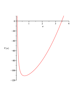
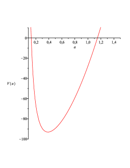
Figure 1: The potential $V(a)$ for $g_{s}=-2$, $g_{r}=120$, $g_{\Lambda}=0$, for $g_{c}=10$ (left) and $g_{c}=90$ (right).

For $g_{c}=10$, we have $\bar{E}=-104.592479205836$. Therefore, from the potential $V(a)$ (Fig. 1), the interval where $\left<a\right>$ oscillates is
$\left[0.3782813789,1.182224715\right]$, which has an amplitude of 0.8039433361. On the other hand, for $g_{c}=90$, we have $\bar{E}=-73.7774376335110$. The interval where $\left<a\right>$ oscillates is $\left[0.2184008560,0.6825577576\right]$, with smaller amplitude, equal to 0.4641569016.

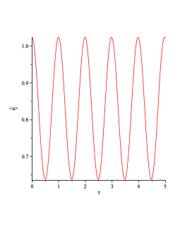
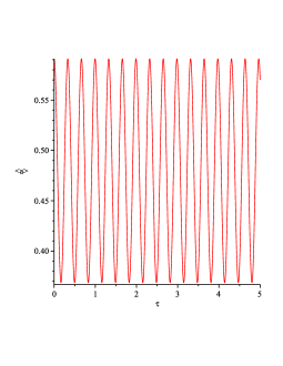
Figure 2: The expected value of the scale factor $\left<a\right>$. Here, $N=2$, $g_{s}=-2$, $g_{r}=120$, $g_{\Lambda}=0$. We show the cases of $g_{c}=10$ (left) and $g_{c}=90$ (right).

3.2.2 Behavior of $\left<a\right>$ as $g_{\Lambda}$ varies

If we fix $N$ and the HL parameters but $g_{\Lambda}$, and let $g_{\Lambda}$ decrease, we observe that: ($i$) the maximum value of $\left<a\right>$ decreases; ($ii$) the amplitude of oscillation of $\left<a\right>$ decreases; ($iii$) the number of oscillations of $\left<a\right>$, for a fixed interval of $\tau$, increases.

That behavior may be understood by the observation of the potential that confines the scale factor. As $g_{\Lambda}$ decreases, $\left<a\right>$ is forced to oscillate within an ever smaller region. Under those conditions, for fixed $N$ and the other HL parameters, the maximum value and the amplitude of $\left<a\right>$ both decrease. Moreover, since the interval where $\left<a\right>$ oscillates is smaller, the number of oscillations of $\left<a\right>$ for a fixed $\tau$ interval also increases. Figs. 3 and 4 illustrate the behavior of the potential $V(a)$ and of the expected value $\left<a\right>$, for two different values of $g_{\Lambda}$ whereas the $\tau$ interval, $N$ and the other HL parameters remain fixed.

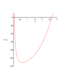
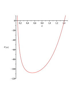
Figure 3: The potential $V(a)$ for $g_{s}=-2$, $g_{r}=120$, $g_{c}=10$. We have used $g_{\Lambda}=-1$ (left) and $g_{\Lambda}=-25$ (right).

For $g_{\Lambda}=-1$, we have $\bar{E}=-103.833980119716$. Therefore, from the potential $V(a)$ (Fig. 3), the interval where $\left<a\right>$ oscillates is
$\left[0.3676565615,1.137772203\right]$, which has an amplitude of 0.7701156415. On the other hand, for $g_{\Lambda}=-25$, we have $\bar{E}=-95.6220677191430$. The interval where $\left<a\right>$ oscillates is $\left[0.2927449802,0.8679732690\right]$, with smaller amplitude, equal to 0.5752282888.

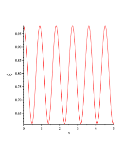
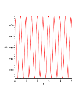
Figure 4: The expected value of the scale factor $\left<a\right>$ for $N=2$, $g_{s}=-2$, $g_{r}=120$, $g_{c}=10$. We have used $g_{\Lambda}=-1$ (left) and $g_{\Lambda}=-25$ (right).

3.2.3 Behavior of $\left<a\right>$ as $g_{r}$ varies

If we fix $N$ and the HL parameters but $g_{r}$, and let $g_{r}$ vary, we observe that the maximum value, the amplitude of oscillation and the number of oscillations of $\left<a\right>$ all remain constant. This is because as $g_{r}$ varies, the amplitude of the interval in which $\left<a\right>$ can oscillate is unaltered. Figs. 5 and 6 show examples of how $\left<a\right>$ behaves for two different values of $g_{r}$, whereas the $\tau$ interval, $N$ and the other HL parameters remain fixed.

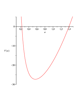
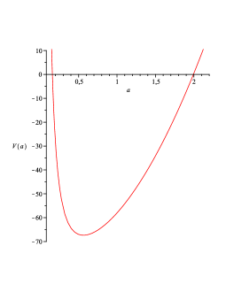
Figure 5: The potential $V(a)$ for $g_{s}=-2$, $g_{\Lambda}=0$, $g_{c}=20$. We have used $g_{r}=40$ (left) and $g_{r}=80$ (right).

For $g_{r}=40$, we have $\bar{E}=-18.2104751421654$. Therefore, from the potential $V(a)$ (Fig. 5), the interval where $\left<a\right>$ oscillates is
$\left[0.3180954556,0.9941285249\right]$, which has an amplitude of 0.6760330693. On the other hand, for $g_{r}=80$, we have $\bar{E}=-58.2104751421655$. The interval where $\left<a\right>$ oscillates is $\left[0.3180954556,0.9941285249\right]$, which has an amplitude of 0.6760330693. Identical to the case $g_{r}=40$.

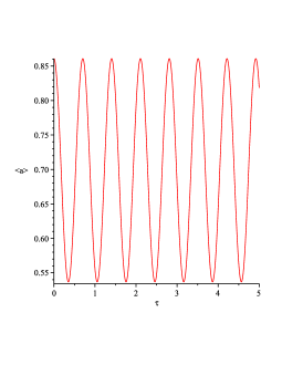
Figure 6: The expected value of the scalar factor $\left<a\right>$ for $N=2$, $g_{s}=-2$, $g_{\Lambda}=0$, $g_{c}=20$. We have used $g_{r}=40$ (left) and $g_{r}=80$ (right).

3.2.4 Behavior of $\left<a\right>$ as $g_{s}$ varies

If we fix $N$ and the HL parameters but $g_{s}$, by letting $g_{s}$ vary, we observe that: (i) both the amplitude and the number of oscillation of $\left<a\right>$, for a fixed $\tau$ interval, remain the same; (ii) the maximum value of $\left<a\right>$ increases as $g_{s}$ decreases.

That behavior may be understood by the observation of the potential that confines the scale factor. As $g_{s}$ decreases, the interval of oscillation of $\left<a\right>$ is unaltered. Under those conditions, for fixed $N$ and the other HL parameters, neither the amplitude nor the number of oscillations of $\left<a\right>$ vary. Notwithstanding, decreasing $g_{s}$ the interval of oscillation of $\left<a\right>$ shifts to the right; hence the maximum value of $\left<a\right>$ gets larger. Figs. 7 and 8 illustrate the behavior of the potential $V(a)$ and of the expected value $\left<a\right>$, for two different values of $g_{s}$ whereas the $\tau$ interval, $N$ and the other HL parameters remain fixed.

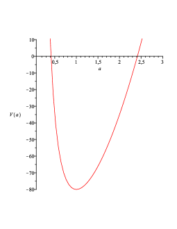
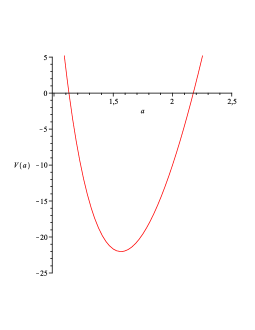
Figure 7: The potential $V(a)$ for $g_{\Lambda}=0$, $g_{r}=120$, $g_{c}=20$. We have used $g_{s}=-20$ (left) and $g_{s}=-120$ (right).

For $g_{s}=-20$, we have $\bar{E}=-70.9932768412420$. Therefore, from the potential $V(a)$ (Fig. 7), the interval where $\left<a\right>$ oscillates is
$\left[0.7192555414,1.390326445\right]$, which has an amplitude of 0.6710709036. On the other hand, for $g_{s}=-120$, we have $\bar{E}=-13.0506261790150$. The interval where $\left<a\right>$ oscillates is $\left[1.265657001,1.935350368\right]$, with amplitude equal to 0.669693367.

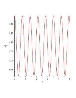
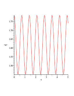
Figure 8: The expected value $\left<a\right>$ of the scale factor for $N=2$, $g_{\Lambda}=0$, $g_{r}=120$, $g_{c}=20$. We have used $g_{s}=-20$ (left) and $g_{s}=-120$ (right).

3.2.5 Behavior of $\left<a\right>$ as $N$ varies

If we fix all the HL parameters but let $N$ increase, we observe that: ($i$) the maximum value of $\left<a\right>$ increases; ($ii$) the amplitude of oscillation of $\left<a\right>$ increases; ($iii$) the number of oscillations of $\left<a\right>$, for a fixed interval of $\tau$, remains constant.

That behavior may be understood by the observation that the mean energy associated with the wavepacket increases with the increase of $N$. As $N$ increases, $\left<a\right>$ oscillates in a ever larger region; hence its maximum value and the amplitude of the oscillation interval of $\left<a\right>$ both increase. The number of oscillations of $\left<a\right>$ for a fixed $\tau$ interval does not change, though. Although the mean energy increases, the potential energy does not vary; hence only the kinetic energy increases. Therefore, $\left<a\right>$ oscillates more rapidly in a larger region. The most interesting result is that the oscillation velocity increases in such way that the oscillation frequency remains constant, as $N$ is increased.

Fig. 1 provides an example for the potential $V(a)$, and Figs. 2 and 9 for $\left<a\right>$, for fixed values of the HL parameters but with different values of $N$.

For $g_{c}=10$, with $N=5$, we have $\bar{E}=-95.1047199335060$. Therefore, from the potential $V(a)$ (Fig. 1), the interval where $\left<a\right>$ oscillates is $\left[1.551262998,0.2882899909\right]$, which has an amplitude of 1.262973007. On the other hand, for $g_{c}=10$ and $N=10$, we have $\bar{E}=-79.2852819937343$. The interval where $\left<a\right>$ oscillates is $\left[2.005428161,0.2230015536\right]$, with amplitude, equal to 1.782426607. Those results must be compared to the results shown in Figs. 1 and 2, in which $g_{c}=10$ and $N=2$.

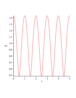
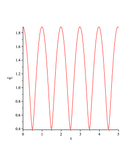
Figure 9: The expected value $\left<a\right>$ of the scale factor for $g_{c}=10$, $g_{\Lambda}=0$, $g_{r}=120$, $g_{s}=-2$. We have used $N=5$ (left) and $N=10$ (right).

3.2.6 Results for the standard deviations

We calculated $\underline{a}=\left<a\right>-\sigma_{a}$, in which $\left<a\right>$ is given by Eq.(35) and $\sigma_{a}$ by Eq.(36), for different ranges of the HL parameters ($g_{c}$, $g_{r}$, $g_{s}$, $g_{\Lambda}$) and values of $N$. For all computed cases, $\underline{a}$ is always positive, thus giving a stronger indication that the present models are free from singularities at the quantum level. As for the mathematical significance of that result, we should mention that if our probability distribution were a normal one and if one took the interval $[\left<a\right>-\sigma_{a},\left<a\right>+\sigma_{a}]$, symmetric about the mean value $\left<a\right>$, it would cover $68,26\%$ of the area under the distribution curve [55]. Fig. 10 shows two examples of how $\left<a\right>$ and $\underline{a}$ evolve with time.

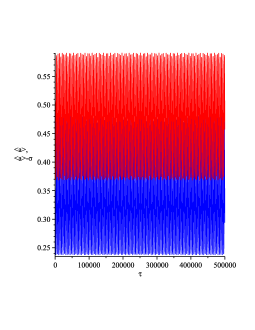
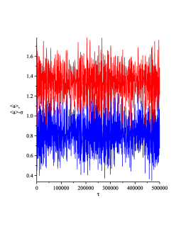
Figure 10: The functions $\left<a\right>$ and $\underline{a}=\left<a\right>-\sigma_{a}$. during the time interval $0<\tau<500000$. Left: we have used $g_{c}=90$, $g_{r}=120$, $g_{\Lambda}=0$, $g_{s}=-2$ and $N=2$. Right: we have used $g_{s}=-20$, $g_{r}=120$, $g_{\Lambda}=0$, $g_{c}=20$ and $N=10$.

4 DeBroglie-Bohm Interpretation

In this section we approach the HL quantum cosmological model using the DeBroglie-Bohm interpretation of quantum mechanics [26, 27]. There are several works in quantum cosmology that have employed such interpretation [23, 28, 29, 30, 31, 32, 33, 34, 35]. We aim at comparing results obtained from this interpretation with that of the Many Worlds interpretation, mainly that the model is free from singularities at the quantum level.

The first step of applying DeBroglie-Bohm interpretation is that of rewriting the quantum cosmological wavefunction $\Psi(a,\tau)$ in its polar form [27]

$$\Psi(a,\tau)=R(a,\tau)e^{iS(a,\tau)},$$ (38)

in which $R(a,\tau)$ and $S(a,\tau)$ are the amplitude and phase of the wavefunction, respectively. Equations for $R(a,\tau)$ and $S(a,\tau)$ can be obtained by inserting $\Psi(a,\tau)$ of Eq. (38) into Eq. (21). Following Refs. [27] and [56], we then obtain two independent equations: one from the real part,

$$\left(\frac{\partial S(a,\tau)}{\partial a}\right)^{2}+Q(a,\tau)+4\left(g_{c}ka^{2}-g_{\Lambda}a^{4}-g_{r}k^{2}-\frac{g_{s}k}{a^{2}}\right)=0,$$ (39)

and another from the imaginary part,

$$2\frac{\partial{R(a,\tau)}}{\partial a}\frac{\partial S(a,\tau)}{\partial a}+R(a,\tau)\frac{\partial^{2}S(a,\tau)}{\partial a^{2}}+\frac{4}{a^{3\omega-1}}\left(\frac{\partial R(a,\tau)}{\partial\tau}\right)=0.$$ (40)

In Eq. (39), the function $Q(a,\tau)$ is known as the Bohmian quantum potential. From the calculations leading to Eq. (39) one obtains that $Q(a,\tau)$ is given by,

$$Q(a,\tau)=-\frac{1}{R(a,\tau)}\frac{\partial^{2}R(a,\tau)}{\partial a^{2}}.$$ (41)

The Bohmian trajectory of the scale factor $a$ is [27]

$$\frac{da(\tau)}{d\tau}=\frac{1}{M}\frac{\partial S}{\partial a},$$ (42)

in which, from Eq. (16), we have the mass $M=2$.

In DeBroglie-Bohm interpretation, the quantum behavior of the Universe is described by the solution of Eq. (42). To each given initial value of $a(\tau)$ corresponds a deterministic scale factor trajectory, representing the evolution of the Universe at the Planck scale.

4.1 Bohmian trajectories of the scale fator $a$

Using the wavepacket determined in Eq. (26), we have obtained its polar form, Eq. (38), identifying its amplitude and phase. Inserting its phase $S(a,\tau)$ in Eq. (42), we computed the Bohmian trajectories of $a$, for different values of all HL parameters. We have used here the same procedure as that of the previous section, in order to investigate how the Bohmian trajectories of $a$ depend on the HL parameters. We fixed all parameters but one, and let that parameter vary over a wide range of values. Then, we repeated the calculation, in the same manner, for all HL parameters. Eq. (42) has been solved, then, for many different values of $g_{c}$, $g_{\Lambda}$, $g_{r}$, $g_{s}$ and $N$. For all values, the qualitative behavior of the Bohmian trajectories of $a(\tau)$ were the same. They oscillate between maxima and minima values and never vanished. Therefore, in the same way as in the Many Worlds interpretation, as we saw in the previous section, in the DeBroglie-Bohm interpretation those models are free from singularities. We have also noticed that the Bohmian trajectories of $a$ are, qualitatively, very similar to the corresponding expected values of $a$. That result helps verifying the equivalence between both quantum mechanical interpretations.

In what follows, we compare some Bohmian trajectories of $a$ with their corresponding expected values of $a$. In order to better compare those two quantum mechanical interpretations we used, for each model, as initial conditions for $a(\tau)$ at $\tau=0$, in the Bohmian trajectories of $a$, the expected values of $a$ at $\tau=0$.

4.1.1 Bohmian trajectories of $a$ as $g_{c}$ varies

Solving equation (42) for several different values of $g_{c}$, $N$ and various $\tau$ intervals, while keeping fixed the other HL parameters, we have observed the following properties of the Bohmian trajectories of $a$, as $g_{c}$ increases: ($i$) the maximum value of $a$ decreases; ($ii$) the amplitude of oscillation of $a$ decreases; ($iii$) the number of oscillations of $a$, for a fixed $\tau$ interval, increases. Such behavior, exemplified in Figs. 2 and 11, agrees with that of the expected value $\left<a\right>$, described in the previous section.

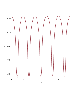
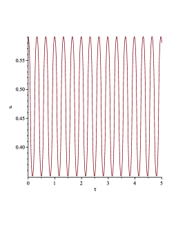
Figure 11: Bohmian trajectories of $a$ for $N=2$, $g_{s}=-2$, $g_{r}=120$, $g_{\Lambda}=0$. Left: we have $g_{c}=10$. Right: we have $g_{c}=90$.

4.1.2 Bohmian trajectories of $a$ as $g_{\Lambda}$ varies

Solving equation (42) for several different values of $g_{\Lambda}$, $N$ and various $\tau$ intervals, while keeping fixed the other HL parameters, we have observed the following behavior of the Bohmian trajectories of $a$, as $g_{\Lambda}$ decreases: ($i$) the maximum value of $a$ decreases; ($ii$) the amplitude of oscillation of $a$ decreases; ($iii$) the number of $a$ oscillations, for a fixed $\tau$ interval, increases. Such behavior of the Bohmian trajectories agrees with that of the expected value $\left<a\right>$, obtained in the previous section. Figures 4 and 12 exemplify such agreement.

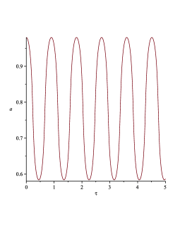
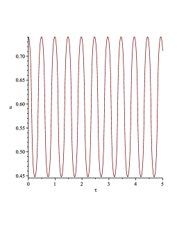
Figure 12: Bohmian trajectories of $a$ for $N=2$, $g_{s}=-2$, $g_{r}=120$, $g_{c}=10$. Left: we have $g_{\Lambda}=-1$. Right: we have $g_{\Lambda}=-25$.

4.1.3 Bohmian trajectories of $a$ as $g_{r}$ varies

Solving equation (42) for several different values of $g_{r}$, $N$ and various $\tau$ intervals, while keeping fixed the other HL parameters, we have observed that the maximum value, the amplitude of oscillation and the number of $a$ oscillations do not vary as $g_{r}$ varies, for a fixed $\tau$ interval. Such behavior agrees with that of the expected value of $a$, obtained in the previous section. Figs. 6 and 13 illustrate that agreement.

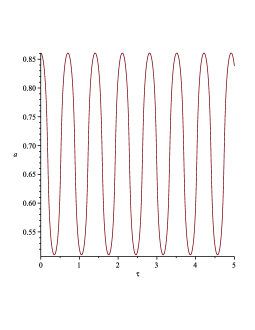
Figure 13: Bohmian trajectories of $a$ for $N=2$, $g_{s}=-2$, $g_{\Lambda}=0$, $g_{c}=20$. Left: we have $g_{r}=40$. Right: we have $g_{r}=80$.

4.1.4 Bohmian trajectories of $a$ as $g_{s}$ varies

Solving equation (42) for several different values of $g_{s}$, $N$ and various $\tau$ intervals, while keeping fixed the other HL parameters, we have observed the following behavior of the Bohmian trajectories of $a$, as $g_{s}$ varies: ($i$) the amplitude of oscillation and the number of oscillations of $a$, for a fixed $\tau$ interval, do not vary; ($ii$) the maximum value of $a$ increases as $g_{s}$ decreases. Such behavior agree with that of expected value $\left<a\right>$, obtained in the previous section. This is exemplified by Figs. 8 and 14.

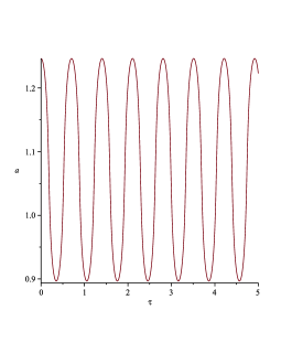
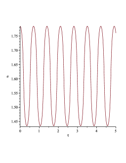
Figure 14: Bohmian trajectories of $a$ for $N=2$, $g_{r}=120$, $g_{\Lambda}=0$, $g_{c}=20$. Left: we have $g_{s}=-20$. Right: we have $g_{s}=-120$.

4.2 The Bohmian quantum potential

Observing the quantum potential $Q(a,\tau)$ in Eq. (41) for the present models, it is not difficult to understand why they are free from singularities. Here, together with the Bohmian trajectories of $a$, we have also computed the potential $Q(a,\tau)$ for many different values of $g_{c}$, $g_{\Lambda}$, $g_{r}$, $g_{s}$ and $N$. The calculations have been made over each Bohmian trajectory of $a$. For all situations considered, we obtained the same qualitative behavior for $Q(a,\tau)$.

If we compute the quantum potential $Q$ as a function of $\tau$ only, we see that it oscillates between maximum and minimum values. There are two different types of maximum values: the absolute maxima and the local maxima. The absolute maxima values are greater than the local maxima values. The absolute maxima of $Q$ occur as the scale factor reaches its minimum values. Therefore, $Q(a,\tau)$ prevents $a(\tau)$ from ever vanishing. On the other hand, the local maxima of $Q$ occur as the scale factor reaches its maximum values. In this way, the quantum potential prevents the scale factor from reaching infinite values. We have also computed $Q(a,\tau)$ as a function of $a$ only. In that case, for all considered values of $g_{c}$, $g_{\Lambda}$, $g_{r}$, $g_{s}$ and $N$, we have observe the same type of quantum potential curve. The absolute and local maxima values of $Q$ can be clearly identified in that curve. Fig. 15 exemplifies the Bohmian quantum potential Eq. (41) for the model with $g_{\Lambda}=-1$, $g_{c}=10$, $g_{r}=120$, $g_{s}=-2$ and $N=2$. In the left panel of Fig. 15, $Q$ is shown as a function of the time $\tau$; in the right panel, $Q$ is shown as a function of $a$. For a better understanding of the behavior of $Q$ it is important to observe the Bohmian trajectory of $a$ plotted on the left panel of Fig. 12. The same time interval used for $a$ in Fig. 12 has been used for $Q$ in Fig. 15, and the initial condition $a(\tau=0)$ for that trajectory was given by the expected value of $a$ at $\tau=0$, for the same model.

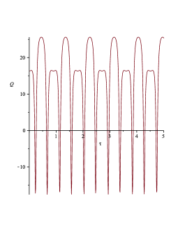
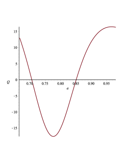
Figure 15: Left: the quantum potential $Q$ as a function of the time $\tau$. Right: the quantum potential $Q$ as a function of the scale factor $a$. In both panels, we have $g_{\Lambda}=-1$, $N=2$, $g_{c}=10$, $g_{r}=120$ and $g_{s}=-2$. The potential $Q$ shown has been computed along the Bohmian trajectory of $a$ presented on the left panel of Fig. 12.

5 Conclusions

In the present paper, we canonically quantized a homogeneous and isotropic Hořava-Lifshitz cosmological model, with constant positive spatial sections and coupled to radiation. We considered the projectable version of that gravitational theory without the detailed balance condition. We used the ADM formalism to write the gravitational Hamiltonian of the model and the Schutz variational formalism to write the perfect fluid Hamiltonian. We obtained the Wheeler-DeWitt equation for the model, which depends on several parameters coming from the HL theory. We studied the case of bounded solutions to the Wheeler-DeWitt equation, and the HL parameters have been chosen accordingly.

First, we have solved it using the Many Worlds interpretation of quantum mechanics. Using wavepackets computed with the solutions to the Wheeler-DeWitt equation, we obtained the expected value of the scalar factor $\left<a\right>$. We showed that this quantity oscillates between maximum and minimum values and never vanishes, indicating that the model is free from singularities, at the quantum level. We have also reinforced this indication by showing that if we subtract a standard deviation unit of $a$ from the expected value $\left<a\right>$, a positive value is still obtained. We have also studied how the expected value of scale factor depends on each of the HL parameters and $N$.

Then we have used the DeBroglie-Bohm interpretation of quantum mechanics. First, by computing the Bohmian trajectories of $a$, for many different values of the HL parameters and $N$. We showed that $a$, for all those trajectories, oscillates between maximum and minimum values and never vanish, in agreement with the behavior of the expected value of $a$. We were able to evaluate how those trajectories depend on the HL parameters and $N$ and compare the Bohmian trajectories of $a$ to the expected value $\left<a\right>$, showing that they agree for the corresponding models. Finally, we computed the quantum potential $Q$, for many different values of the HL parameters and $N$, showing how that quantity helps understanding why the scale factor never vanishes, in the present HL cosmological model.

References

- [1] B. P. Abbott et al., Phys. Rev. Lett. 116, 061102 (2016).
- [2] For a complete list of references see: S. W. Hawking and G. F. R. Ellis, The large scale structure of space-time, (Cambridge University Press, Cambridge, 1973).
- [3] For an introduction to this subject see: S. Weinberg, in General Relativity. An Einstein Centenary Survey, edited by S. W. Hawking and W. Israel (Cambridge University Press, Cambridge, 1980).
- [4] K. S. Stelle, Phys. Rev. D 16, 953 (1977).
- [5] P. Hořava, Phys. Rev. D 79, 084008 (2009).
- [6] S. K. Ma, Modern Theory of Critical Phenomena, (Benjamin, New York, 1976).
- [7] P. C. Hohenberg and B. I. Halperin, Rev. Mod. Phys. 49, 435 (1977).
- [8] S. Sachdev, Quantum Phase Transitions (Cambridge University Press, Cambridge, U.K., 1999).
- [9] E. Ardonne, P. Fendley and E. Fradkin, Ann. Phys. (N. Y.) 310, 493 (2004).
- [10] R. Arnowitt, S. Deser and C. W. Misner, in Gravitation: an introduction to current research, ed. L. Witten (Wiley, New York, 1962), Chapter 7, pp 227-264 and arXiv:gr-qc/0405109.
- [11] D. Blas, O. Pujolas and S. Sibiryakov, Consistent extension of Hořava gravity, Phys. Rev. Lett. 104, 181302 (2010).
- [12] D. Blas, O. Pujolas and S. Sibiryakov, On the extra mode and inconsistency of Hořava-Lifshitz, JHEP 04, 018 (2011).
- [13] T. P. Sotiriou, M. Visser and S. Weinfurtner, Phenomenologically viable Lorentz-violating quantum gravity, Phys. Rev. Lett. 102, 251601 (2009).
- [14] T. P. Sotiriou, M. Visser and S. Weinfurtner, Quantum gravity without Lorentz invariance, JHEP 10, 033 (2009).
- [15] A. Wang and R. Maartens, Linear perturbation of cosmological models in the Hořava-Lifshitz theory of gravity without detailed balance, Phys. Rev. D 81, 024009 (2010).
- [16] O. Bertolami and C. A. D. Zarro, Hořava-Lifshitz quantum cosmology, Phys. Rev. D 84, 044042 (2011).
- [17] J. P. M. Pitelli and A. Saa, Quantum singularities in Hořava-Lifshitz cosmology, Phys. Rev. D 86, 063506 (2012).
- [18] B. Vakili and V. Kord, Classical and quantum Hořava-Lifshitz cosmology in a minisuperspace perspective, Gen. Relativ. Gravit. 45, 1313 (2013).
- [19] H. Ardehali and P. Pedram, Chaplygin gas Hořava-Lifshitz quantum cosmology, Phys. Rev. D 93, 043532 (2016).
- [20] Y. Misonoh, M. Fukushima and S. Miyashita, Stability of singularity-free cosmological solutions in Hořava-Lifshitz gravity, Phys. Rev. D 95, 044044 (2017).
- [21] R. Maier and I. D. Soares, Hořava-Lifshitz bouncing Bianchi IX Universes: A dynamical system analysis, Phys. Rev. D 96, 103532 (2017).
- [22] S. F. Bramberger et al, Solving the flatness problem with an anisotropic instanton in Hořava-Lifshitz gravity, Phys. Rev. D 97, 043512 (2018).
- [23] G. Oliveira-Neto, L. G. Martins, G. A. Monerat and E. V. Corrêa Silva, De Broglie-Bohm interpretation of a Hořava-Lifshitz quantum cosmology model, Mod. Phys. Lett. A 33, 1850014 (2018).
- [24] A. Wang, Hořava gravity at a Lifshitz point: A progress report, Int. J. Mod. Phys. D 26, 1730014 (2017).
- [25] H. Everett, Relative state formulation of quantum mechanics, Rev. Mod. Phys. 29, 454 (1957).
- [26] D. Bohm and B. J. Hiley, The undivided Universe: an ontological interpretation of quantum theory, Routledge, London, 1993;
- [27] P. R. Holland, The quantum theory of motion: an account of the de Broglie-Bohm interpretation of quantum mechanics, Cambridge University Press, Cambridge, 1993.
- [28] S. P. Kim, Phys. Lett. A 236, 11 (1997).
- [29] J. Acacio de Barros, N. Pinto-Neto and M. A. Sagioro-Leal, Phys. Lett. A 241, 229 (1998).
- [30] P. Pedram and S. Jalalzadeh, Phys. Lett. B 660, 1 (2008).
- [31] G. A. Monerat, L. G. Ferreira Filho, G. Oliveira-Neto, E. V. Corrêa Silva, C. Neves, Phys. Lett. A 374, 4741 (2010).
- [32] B. Vakili, Phys. Lett. B 718, 34 (2012).
- [33] S. Das, Phys. Rev. D 89, 084068 (2014).
- [34] A. F. Ali and S. Das, Phys. Lett. B 741, 276 (2015).
- [35] G. Oliveira-Neto, M. Silva de Oliveira, G. A. Monerat and E. V. Corrêa Silva, Int. J. Mod. Phys. D 26, 1750011 (2016).
- [36] N. Pinto-Neto and J. C. Fabris, Class. Quantum Grav. 30, 143001 (2013).
- [37] Dongshan He, Dongfeng Gao and Qing-yu Cai, Phys. Rev. D 89, 083510 (2014).
- [38] Dongshan He, Dongfeng Gao and Qing-yu Cai, Phys. Lett. B 748, 361 (2015).
- [39] A. G. Riess et al. Astron. J. 116, 1009 (1998); S. Perlmutter et al., Astrophys. J. 517, 565 (1999).
- [40] C. W. Misner, K. S. Thorne and J. A. Wheeler, Gravitation, (W. H. Freeman and Company, New York, 1973).
- [41] Schutz, B. F., Phys. Rev. D 2, 2762, (1970).
- [42] Schutz, B. F., Phys. Rev. D 4, 3559, (1971).
- [43] F.G. Alvarenga, J.C. Fabris, N.A. Lemos and G.A. Monerat, Gen. Rel. Grav. 34, 651 (2002).
- [44] V. G. Lapchinskii and V. A. Rubakov, Theor. Math. Phys. 33, 1076 (1977).
- [45] P. A. M. Dirac, Can. J. Math. 2, 129 (1950); Proc. Roy. Soc. London A 249, 326 and 333 (1958); Phys. Rev. 114, 924 (1959).
- [46] N. A. Lemos, J. Math. Phys. 37, 1449 (1996).
- [47] J. P. Boyd. Chebyshev and Fourier Spectral Methods. 2nd ed., New York, Dover (2001).
- [48] P. Pedram, M. Mirzaei, S. Jalalzadeh, S.S. Gousheh. Gen. Rel. Grav. 40, 1663 (2008).
- [49] G. Oliveira-Neto, G. A. Monerat, E. V. Corrêa Silva, C. Neves and L. G. Ferreira Filho, Int. J. Theor. Phys. 52, 2991 (2013).
- [50] E. V. Corrêa Silva, G. A. Monerat, G. Oliveira-Neto and L. G. Ferreira Filho, Comput. Phys. Commun. 185, 380 (2014).
- [51] R. F. Aranha, I. D. Soares and E. V. Tonini, Phys. Rev. D 85, 024003 (2012).
- [52] J. Celestino, H. P. de Oliveira and E. L. Rodrigues, Phys. Rev. D 93, 104018 (2016).
- [53] P. C. M. Clemente and H. P. de Oliveira, Phys. Rev. D 96, 024035 (2017).
- [54] W. Barreto, P. C. M. Clemente, H. P. de Oliveira and B. R. Mueller, Phys. Rev. D 97, 104035 (2018).
- [55] P. L. Meyer, Introductory Probability and Statistical Applications, (Addison-Wesley, Reading, 1970).
- [56] S. P. Kim, Phys. Rev. D 55, 7511 (1997).