Reconstructing braneworld inflation

Abstract

The reconstruction of a braneworld inflationary universe considering the parametrization (or attractor) of the scalar spectral index $n_{s}(N)$ in terms of the number of $e$-foldings N is developed. We also study the possibility that the reconstruction for the scenario of braneworld inflation, can be realized in terms of the tensor to scalar ratio $r(N)$. For both reconstruction methodologies, we consider a general formalism in order to obtain the effective potential as a function of the cosmological parameters $n_{s}(N)$ or $r(N)$. For both reconstruction methods, we consider the specific examples for large $N$ in the framework of the slow roll approximation as; the attractor $n_{s}-1\propto N^{-1}$ for the scalar spectral index and the attractor $r\propto N^{-2}$ for the tensor to scalar ratio. In this context and depending on the attractors used, we find different expressions for the effective potential $V(\phi)$, as also the constraints on the parameters present in the reconstruction.

I Introduction

It is well known that during the early universe, the introduction of the inflationary stage or inflation, is to date a possible solution to many long-standing problems of the hot big bang model (horizon, flatness, monopoles, etc.)Staro ; guth ; infla . However, the most significant characteristic of the inflationary model is that inflation gives account of a causal interpretation of the origin of the observed anisotropy of the cosmic microwave background radiation (CMB), as also the distribution of a large scale structure observed todayA1 ; astro ; astro2 ; Planck2018 .

In order to describe the inflationary epoch for the early universe, different inflationary models have been proposed in the framework of General Relativity (GR) as in modified gravity or an alternative to Einstein’s General Relativity. In this context, implications of string/M-theory to Friedmann-Robertson-Walker (FRW) cosmological models have attracted a great deal of attention in the last years and in particular some models with brane-antibrane configurations like some time-like branes, together with their applications to the inflationary cosmologysen1 . In this framework, the introduction of extra dimensions generates extra terms in the Friedmann equation product of the dimensional reduction (embedded) to four-dimensions 1 ; 3 ; 8 and the standard model of particles is confined to the brane, while the gravitation propagates into the bulk space-time3 . In this respect, the inflationary model of a Randall-Sundrum (RS) type II scenario has taken great attentiveness in the last yearsRS and this modification to GR for the cosmological models has been widely studied. In particular the chaotic model on the brane in the framework of slow roll was analyzed in Ref.Maartens:1999hf . In Ref.Huey:2001ae an inverse power law potential was studied, where a single scalar field can act as an inflaton field and quintessence for an appropriate value of the brane tension. In the case of a tachyonic potential considering the power law inflation in the frame of braneworld cosmology was developed in Ref.Sami:2002zy . For a comprehensible review of brane-cosmology, see e.g. Refs.4 ; 5 ; M1 and recent articles; see the list in Kallosh:2018zsi .

On the other hand, the reconstruction of the background and in particular the effective potential associated with a scalar field in the context of inflation from observational data such as the scalar spectrum, scalar spectral index $n_{s}$ and the tensor to scalar ratio $r$, has been analyzed by several authors Hodges:1990bf ; HL1 ; H2 ; H3 ; H4 ; Chiba:2015zpa ; H5 . Originally, considering a single scalar as the reconstruction of inflationary potentials from the primordial scalar spectrum was proposed in Ref.Hodges:1990bf .

An attractive mechanism to reconstruct the effective potential of the scalar field assuming the slow roll approximation is through the parametrization in terms of the number of $e$-folds $N$. In this respect, by considering the scalar spectral index $n_{s}(N)$ and the tensor to scalar ratio $r(N)$ (commonly called attractors) it is possible to reconstruct the background during the inflationary epoch. From an observational point of view, the attractors given by $n_{s}-1\propto N^{-1}$ and $r\propto N^{-2}$, by considering the number of $e$-foldings $N\simeq 50-70$ at the end of the inflationary epoch, agree with the Planck resultsPlanck2018 . In particular and considering the framework of GR the scalar spectral index given by $n_{s}(N)-1\propto N^{-1}$, it is possible to build different effective potentials such as; the T-model T , E-modelE , Staronbisky $R^{2}$-modelStaro , the chaotic modelLinde83 and the model of Higgs inflation with non minimal couplingHiggs ; Higgs2 . In the framework of warm inflation unlike cold inflation, it was necessary to consider jointly the attractors $n_{s}(N)$ and $r(N)$, in order to reconstruct the effective potential and the dissipation coefficient Herrera:2018cgi . Analogously, the reconstruction of an inflationary model in the context of the Galileon model or G-model, considering as attractors the scalar spectral index and the tensor to scalar ratio as a function of the number of $e$-folding jointly was studied in Ref.Herrera:2018kera .

We also mentioned another way to reconstruct the background and it is related with the slow-roll parameter $\epsilon$ and its parametrization in terms of $N$ i.e., $\epsilon(N)$. In this sense, considering $\epsilon(N)$ is possible to find the scalar spectral index and the tensor to scalar ratio for inflationary models in GR, see Huang:2007qz ; Gao:2017owg . In particular choosing different slow-roll parameters $\epsilon(N)$, the reconstruction of several effective potentials associated with a scalar field and the observational parameters were studied in Ref.M1 . Also, in Refs.Roest:2013fha ; N1 ; N2 were found the effective potential and the consistency relation $r=r(n_{s})$, but considering the two slow roll parameters $\epsilon(N)$ and $\eta(N)$.

In the context of modified gravity, in Ref.Odintsov:2018zhw the reconstruction of the effective potential and the coupling of the Gauss-Bonnet function was obtained during the inflationary epoch by fixing the tensor-to-scalar ratio and the Hubble parameter as a function of the $e$-folds, in the framework of Einstein Gauss-Bonnet gravity. Also, the reconstruction of an inflationary stage assuming the slow-roll approximation for $F(R)$ gravity considering different expressions for the tensor to scalar ratio in terms of $N$, was developed in Ref.Odintsov:2017fnc , see also Ref.Odintsov:2018ggm for other modified gravities.

On the other hand, the reconstruction technique from different Equation of State (EoS) in the context of the fluid cosmology during inflation was studied in Refs.fluido ; fluidoA ; expo and for the case of the current universe in fluido2 . In particular for the reconstruction of the inflationary epoch it is possible to assume an ansatz on the effective EoS as function of the number of $e-$foldingsfluido . Here, rewriting the scalar spectral index and the tensor to scalar ratio in terms of the effective EoS, one can find the attractors $n_{s}(N)$ and $r(N)$ in the fluid inflation. Subsequently, if the fluid corresponds to a standard scalar field, one can obtain the reconstruction of the effective potential under slow roll approximationfluido .

It is interesting to mention that from the point of view of the fluid cosmology, it is possible to consider effects of viscosity terms dependent on the Hubble rate and its derivatives in the EoS of the dark fluid and then the equations of motion from this fluid can be visualized as modifications to the GR, which is how it happens in some braneworld models or fourth order gravity, see Ref.Capozziello:2005pa .

Another methodology that has been widely studied in the literature for the reconstruction of the effective potential and the observables $n_{s}(N)$ and $r(N)$ in the framework of inflation is to consider the scale factor as ansatz. In this sense, we mentioned the inflationary models such as; power-lawpowerl , intermediateinterm , logamediateloga , exponential expo ; Herrera:2018ker , among others. Models of dark energy and its reconstruction from the scale factor were studied in Refs.m1 ; m2 .

The goal of this study is to reconstruct the braneworld inflation, through the parametrization of the scalar spectral index or the tensor to scalar ratio, as function of the number of e-foldings. In fact, we analyze how the brane model changes the reconstruction of the scalar potential, considering as attractors the spectral index $n_{s}(N)$ or the tensor to scalar ratio $r(N)$. In this respect, we will consider the domination of the brane effect, in order to obtain analytical solutions in the reconstruction of the background. We will also formulate a general formalism to find the effective potential, by assuming the parametrization $n_{s}(N)$ or $r(N)$, in the context of the slow roll approximation. Thus, choosing a specific attractor for the observable $n_{s}$ or the tensor to scalar ratio $r$ in terms of the number of $e$-folds for large $N$, we will show the possibility of reconstructing the effective potential $V(\phi)$, in the frame of braneworld inflation.

As an application of the formulated formalism, we will analyze two different reconstructions. Following the standard reconstruction of the background from $n_{s}(N)$, we shall consider the specific case in which the scalar spectral index is given by $n_{s}=1-2/N$. As a second reconstruction, we shall regard the reconstruction from the point of view of the tensor to scalar ratio $r(N)$ and as it modifies the reconstruction of the effective potential. In these reconstructions, we will derive different constraints on the parameters present in the models.

The outline of the paper is as follows. The next section presents a brief review of the background and the cosmological perturbations on brane world. In section III, we develop the reconstruction in our model. In Section IV, we consider the high energy limit and the reconstruction, considering the attractor as the scalar spectral index $n_{s}(N)$. Here, we formulate a general formalism to find the effective potential and in Sec. IV.1, we also apply our results to a specific example for the spectral index $n_{s}(N)$. In section V, we formulate the reconstruction from the tensor to scalar ratio $r(N)$ under a general formalism and in subsectionV.1, we consider as example the attractor $r(N)\propto N^{-2}$. Finally, in section VI we summarize our findings. We chose units so that $c=\hbar=1$.

II Braneworld inflation: basic equations

In this section we give a brief review of the background equations and cosmological perturbations on the brane. We begin with the action given by

$$S=M_{5}^{3}\int\,d^{5}x\,\sqrt{G}\left({}^{(5)}R-2\Lambda_{5}\right)-\int\,d^{4}x\,\sqrt{-g}\,L_{matter},$$ (1)

where the quantity ${}^{5}R$ corresponds to the Ricci scalar curvature of the metric $G_{ab}$ of the five dimensional bulk, $L_{matter}$ describes the matter confined on the brane, $M_{5}$ and $\Lambda_{5}$ are the five-dimensional Planck mass and cosmological constant, respectively. The relation between the Planck mass in four dimensional $m_{p}$ and $M_{5}$ and also the relationship between the cosmological constants becomes 2

$$m_{p}=\sqrt{\frac{3}{4\pi}}\,\left(\frac{M_{5}^{2}}{\sqrt{\tau}}\right)M_{5},\,\,\mbox{and}\,\,\,\,\Lambda_{4}=\frac{4\pi}{M_{5}^{4}}\left(\Lambda_{5}+\frac{4\pi}{3M_{5}^{3}}\tau^{2}\right),$$

respectively. Here, $\Lambda_{4}$ corresponds to the four dimensional cosmological constant and the quantity $\tau$ denotes the brane tension.

From the action (1) the authors of Ref.3 have shown that the four dimensional Einstein equations induced on the brane can be written as (see also Ref.RM )

$$G_{\mu\nu}=-\Lambda_{4}\,g_{\mu\nu}+\left(\frac{8\pi}{m_{p}^{2}}\right)\,T_{\mu\nu}+\left(\frac{8\pi}{M_{5}^{2}}\right)S_{\mu\nu}-{\mathcal{E}}_{\mu\nu},$$ (2)

in which $T_{\mu\nu}$ corresponds to the energy-momentum tensor of the matter, the quantity $S_{\mu\nu}$ denotes the local correction to standard Einstein eqs. from the extrinsic curvature and ${\mathcal{E}}_{\mu\nu}$ is the nonlocal effect correction due to a free gravitational field which emerges from the projection of the bulk Weyl tensor. By considering an extended version of Birkhoff’s theorem, we find that if the bulk space-time is anti-de Sitter, then the nonlocal effect corrections ${\mathcal{E}}_{\mu\nu}=0$ B1 and from the Bianchi identity ($\nabla^{\mu}G_{\mu\nu}=0$), we have $\nabla^{\mu}S_{\mu\nu}=0$RM . On the other hand, assuming that the matter in the brane (the matter is confined in the brane and the gravity can be propagated to the extra dimension) is describe by a perfect fluid together with a flat FRW metric, then we find that the modified Friedmann equation becomes 2 ; 3

$$3H^{2}=\kappa\,\rho\left[1+\frac{\rho}{2\tau}\right]+\Lambda_{4}+\frac{\xi}{a^{4}},$$ (3)

where the quantity $H=\dot{a}/a$ denotes the Hubble rate, $a$ corresponds to the scale factor and $\rho$ denotes the matter field confined to the brane. Here, the constant $\kappa=8\pi/m_{p}^{2}$, where $m_{p}$ is the four-dimensional Planck mass. The quantity $\xi/a^{4}$ has a form of dark radiation and it indicates the influence of the bulk gravitons on the brane, in which $\xi$ corresponds to an integration constant. As we emphasized before, the brane tension $\tau$ is related with the four and five dimensional Planck masses by the relation $m_{p}^{2}=3M_{5}^{6}/(4\pi\tau)$ and a constraint on the value of the brane tension is found from nucleosynthesis given by $\tau>$ (1MeV)⁴ Cline . However, a different constraint for the brane tension from current tests for deviation from Newton‘s law was obtained in Refs.test1 ; test2 in which it is restricted to $\tau\geq$(10 TeV)⁴.

In the following, we will consider that the constant $\Lambda_{4}=0$, and once the inflation epoch initiates, the quantity $\xi/a^{4}$ will rapidly become unimportant, with which the modified Friedmann Eq.(3) becomes3

$$3H^{2}=\kappa\,\rho\left[1+\frac{\rho}{2\tau}\right].$$ (4)

In order to describe the matter, we consider that the energy density $\rho$ corresponds to a standard scalar field $\phi$, where the energy density $\rho(\phi)$ and the pressure $P(\phi)$ are defined as $\rho=\frac{\dot{\phi}^{2}}{2}+V(\phi)$, and $P=\frac{\dot{\phi}^{2}}{2}-V(\phi)$, respectively. Here, the quantity $V(\phi)=V$ denotes the scalar potential. We also consider that the scalar field $\phi$ is a homogeneous scalar field i.e., $\phi=\phi(t)$ and also this field is confined to the brane 2 ; 3 . In this context, the dynamics of the scalar field can be written as

$$\dot{\rho}+3H(\rho+P)=0,$$ (5)

or equivalently

$$\ddot{\phi}+3H\dot{\phi}+V^{\prime}=0,$$ (6)

where $V^{\prime}=\partial V(\phi)/\partial\phi$. Here the dots mean derivatives with respect to the cosmological time.

By assuming the slow roll approximation in which the energy density $\rho\sim V(\phi)$, then the Eq.(4) reduces to2 ; 3

$$3H^{2}\approx\kappa\,V\left[1+\frac{V}{2\tau}\right],$$ (7)

and Eq.(6) can be written as

$$3H\dot{\phi}\approx-V^{\prime}.$$ (8)

Following Ref.2 we can introduce the slow roll parameters $\epsilon$ and $\eta$ defined as

$$\epsilon=\frac{1}{2\kappa}\left(\frac{V^{\prime}}{V}\right)^{2}\,\frac{(1+V/\tau)}{(1+V/2\tau)^{2}},\,\,\,\,\,\mbox{and}\,\,\,\,\,\,\,\eta=\frac{1}{\kappa}\frac{V^{\prime\prime}}{V(1+V/2\tau)}.$$ (9)

On the other hand, introducing the number of $e$-folding $N$ between two different values of the time $t$ and $t_{e}$ gives

$$N=\int_{t}^{t_{e}}\,H\,dt\simeq\kappa\int_{\phi_{e}}^{\phi}\,\frac{V}{V^{\prime}}\left(1+\frac{V}{2\tau}\right)\,d\phi,$$ (10)

where $t_{e}$ corresponds to the end of the inflationary stage and here we have considered the slow roll approximation.

In the context of the brane world the power spectrum ${\mathcal{P}_{\mathcal{R}}}$ of the curvature perturbations assuming the slow-roll approximation is given by 4 .

$${\mathcal{P}_{\mathcal{R}}}=\left(\frac{H^{2}}{\dot{\phi}^{2}}\right)\,\left(\frac{H}{2\pi}\right)^{2}\simeq\frac{\kappa^{3}}{12\pi^{2}}\,\frac{V^{3}}{V^{\prime}\,{}^{2}}\,\left(1+\frac{V}{2\tau}\right)^{3}.$$ (11)

The scalar spectral index $n_{s}$ is defined as $n_{s}-1=\frac{d\ln\,{\mathcal{P}_{R}}}{d\ln k}$ and in terms of the slow roll parameters $\epsilon$ and $\eta$ can be written as4

$$n_{s}-1=-6\epsilon+2\eta.$$ (12)

Here we have used Eqs.(9) and (11), respectively.

It is well known that the tensor-perturbation during inflation would produce gravitational waves. In the braneworld the tensor perturbation is more complicated than the standard expression obtained in GR, where the amplitude of the tensor perturbations ${\mathcal{P}}_{g}\propto H^{2}$. Because the braneworld gravitons propagate in the bulk, the amplitude of the tensor perturbation suffers a modification t , wherewith

$${\mathcal{P}}_{g}=8\kappa\,\left(\frac{H}{2\pi}\right)^{2}F^{2}(x),$$ (13)

where the quantity $x=Hm_{p}\sqrt{3/(4\pi\tau)}$ and the function $F(x)$ is defined as

$$F(x)=\left[\sqrt{1+x^{2}}-x^{2}\sinh^{-1}(1/x)\right]^{-1/2},$$ (14)

in which the correction given by the function $F(x)$, appeared from the normalization of a zero-modet . In particular in the limit in which the tension $\tau\gg V$, the function $F(x)\rightarrow 1$ and then ${\mathcal{P}}_{g}\propto H^{2}$.

An important observational quantity is the tensor to scalar ratio $r$, defined as $r=\left(\frac{{\mathcal{P}}_{g}}{P_{\mathcal{R}}}\right)$. Thus, combining Eqs.(11) and (13), the tensor-scalar ratio, $r$, is given by

$$r=\left(\frac{{\mathcal{P}}_{g}}{\mathcal{P}_{\mathcal{R}}}\right)\simeq\frac{8}{\kappa}\left(\frac{V^{\prime}}{V}\right)^{2}\,\left(1+\frac{V}{2\tau}\right)^{-3}\,F^{2}(V).$$ (15)

Here, we have considered that the quantity $x$ can be rewritten in terms of the effective potential from Eq.(7).

III Reconstruction on brane

In this section we consider the methodology in order to reconstruct the background variables, considering the scalar spectral index in terms of the number of $e$-folds in the framework of brane-world. As a first part, we rewrite the scalar spectral index given by Eq.(12), as a function of the number of $e$-folds $N$ and its derivatives. In this form, obtaining the index $n_{s}=n_{s}(N)$, we should find the potential $V=V(N)$ in terms of the number of $e$-folding $N$. Subsequently, utilizing the relation given by Eq.(10), we should obtain the $e$-folds $N$ as a function of the scalar field $\phi$ i.e., $N=N(\phi)$. Finally, considering these relations, we can reconstruct the effective potential $V(\phi)$ in order to satisfy a specific attractor $n_{s}(N)$.

In this way, we start by rewriting the standard slow roll parameters $\epsilon$ and $\eta$ in terms of the number of $e$-folds $N$. Thus, the derivative of the scalar potential $V^{\prime}$ from Eq.(10) can be rewritten as

$$V^{\prime}=\frac{dV}{d\phi}=V_{,\,N}\frac{dN}{d\phi},\,\,\,\,\,\mbox{in which}\,\,\,\,V^{\prime}\,{}^{2}=\kappa V\,\left(1+\frac{V}{2\tau}\right)\,V_{,\,N},$$ (16)

and this suggests that $V_{,\,N}$ is a positive quantity. In the following, we will consider that the notation $V_{,\,N}$ corresponds to $dV/dN$, $V_{,\,NN}$ denotes $d^{2}V/dN^{2}$, etc.

Analogously, we can rewrite $V^{\prime\prime}$ as

$$V^{\prime\prime}=\frac{\kappa}{2V_{,\,N}}\,\left[V_{,\,N}^{2}\,\left(1+\frac{V}{\tau}\right)+V\left(1+\frac{V}{2\tau}\right)V_{,\,NN}\right].$$

In this form, the slow roll parameter $\epsilon$ can be rewritten as

$$\epsilon=\frac{1}{2}\,\frac{\left(1+\frac{V}{\tau}\right)}{V\left(1+\frac{V}{2\tau}\right)}\,\,V_{,\,N},$$ (17)

and the parameter $\eta$ as

$$\eta=\frac{1}{2V}\,\frac{\left(1+\frac{V}{\tau}\right)}{\left(1+\frac{V}{2\tau}\right)}\,V_{,\,N}+\frac{V_{,\,NN}}{2V_{,\,N}}\,\,,$$ (18)

respectively. Here, we have considered that $V^{\prime}>0$.

Also, from Eqs.(10) and (16) we can rewritten $dN/d\phi$ as

$$\frac{dN}{d\phi}=\sqrt{\frac{\kappa V}{V_{,\,N}}}\,\sqrt{\left(1+\frac{V}{2\tau}\right)}\,.$$ (19)

In this way, by using Eq.(12) we find that the scalar spectral index can be rewritten as

$$n_{s}-1=-2\frac{\left(1+\frac{V}{\tau}\right)}{V\left(1+\frac{V}{2\tau}\right)}\,V_{,\,N}+\frac{V_{,\,NN}}{V_{,\,N}},$$ (20)

or equivalently

$$n_{s}-1=-2\left[\ln\left(V\left[1+\frac{V}{2\tau}\right]\right)\right]_{,\,N}+[\ln\,V_{,\,N}]_{,\,N}=\left[\ln\left(\frac{V_{,\,N}}{V^{2}\left(1+\frac{V}{2\tau}\right)^{2}}\right)\right]_{,\,N}.$$ (21)

We also note that in the limit in which $\tau\rightarrow\infty$, Eq.(21) reduces to GR, in which $n_{s}-1=\left(\ln\frac{V_{,\,N}}{V^{2}}\right)_{,\,N}$, see Ref.Chiba:2015zpa .

From Eq.(21) we have

$$\frac{V_{,\,N}}{V^{2}(1+V/2\tau)^{2}}=e^{\int\,{(n_{s}-1)}dN}.$$ (22)

This equation gives us the effective potential $V(N)$ for a specific attractor $n_{s}(N)$. Thus, integrating we have

$$\frac{1}{\tau}\,\ln\left(\frac{1+V/2\tau}{V/2\tau}\right)-\frac{(1+V/\tau)}{V(1+V/2\tau)}=\int\left[e^{\int\,{(n_{s}-1)}dN}\right]\,dN\,.$$ (23)

However, this equation results in a transcendental equation for the scalar potential $V$ and this result does not permit one to obtain the relation $V=V(N)$.

We also note that by combining Eqs.(19) and (22), we obtain that the relation between the number of $e$-folds $N$ and the scalar field $\phi$ can be written as

$$\left[\sqrt{V\,\left(1+\frac{V}{2\tau}\right)}\,e^{\int\,{\frac{(n_{s}-1)}{2}dN}}\right]\,dN=d\phi.$$ (24)

On the other hand, from Eq.(15) the tensor-scalar ratio, $r$ can be rewritten as

$$r(N)\simeq\left(\frac{4}{\tau}\right)\,V_{,\,N}\,\left(1+\frac{V}{2\tau}\right)^{-3}\,F^{2}(V).$$ (25)

In the following we will consider the high energy limit in which $\rho\simeq V\gg\tau$, in order to obtain an analytical solution in the reconstruction of the scalar potential in terms of the scalar field $V(\phi)$.

IV High energy:Reconstruction from the attractor $n_{s}(N)$

In this section we consider the high energy limit ($V\gg\tau$) in order to reconstruct the scalar potential, considering as an attractor the scalar spectral index in terms of the number of $e$-folds i.e., $n_{s}=n_{s}(N)$. In this limit, the derivatives $V^{\prime}$ and $V^{\prime\prime}$ can be rewritten as

$$V^{\prime}\,{}^{2}=\frac{\kappa}{2\tau}\,V^{2}\,V_{,\,N},\,\,\,\,\mbox{and}\,\,\,\,V^{\prime\prime}=\frac{\kappa}{2\tau}\,V\,\left[V_{,\,N}+\frac{V\,V_{,\,NN}}{2V_{,\,N}}\right].$$ (26)

In this way, the relation between the number $N$ and the scalar field $\phi$ in this limit becomes

$$\frac{dN}{d\phi}=\frac{\kappa}{2\tau}\,\left(\frac{V^{2}}{V^{\prime}}\right)=\left(\frac{\kappa}{2\tau}\right)^{1/2}\,\frac{V}{\sqrt{V_{,\,N}}}.$$ (27)

From Eq.(12) we find that the scalar spectral index $n_{s}$ results in

$$n_{s}-1=\frac{4\tau}{\kappa}\left[V^{\prime\prime}-\frac{3V^{\prime}\,{}^{2}}{V}\right]\,\frac{1}{V^{2}}=-4\frac{V_{,\,N}}{V}+\frac{V_{,\,NN}}{V_{,\,N}},$$ (28)

or equivalently

$$n_{s}-1=-4[\ln\,V]_{,\,N}+[\ln V_{,\,N}]_{,\,N}=\left[\ln\left(\frac{V_{,\,N}}{V^{4}}\right)\right]_{,\,N}.$$ (29)

We note that the relation between the scalar potential and the scalar spectral index given by Eq.(29) becomes independent of the brane tension $\tau$ in the high energy limit.

From Eq.(29), the scalar potential in terms of the number of $e$-foldings can be written as

$$V=V(N)=\left[-3\int\left(e^{\int(n_{s}-1)dN}\right)\,dN\right]^{-1/3},$$ (30)

where $\int\left(e^{\int(n_{s}-1)dN}\right)\,dN<0$, in order to make certain that the potential $V(N)>0$.

Now, by combining Eqs.(27) and (29), we find that the relation between $N$ and $\phi$ is given by the general expression

$$\left[V\,e^{\int\frac{(n_{s}-1)}{2}dN}\right]\,dN=\left(\frac{\kappa}{2\tau}\right)^{1/2}\,d\phi,$$ (31)

where $V$ is given by Eq.(30).

In this form, Eqs.(30) and (31) are the fundamental relations in order to build the scalar potential $V(\phi)$ for an attractor point $n_{s}(N)$, in the framework of the high energy limit in brane world inflation.

On the other hand, in the high energy limit in which $V\gg\tau$, the function $F^{2}(x)$ given by Eq.(15) becomes $F^{2}(x)\approx\frac{3}{2}x=\frac{3}{2}\frac{V}{\tau}$. In this form, in the high energy limit the tensor to scalar ratio $r$ becomes

$$r\simeq\,48\tau\,\left(\frac{V_{,\,N}}{V^{2}}\right).$$ (32)

Here we have considered Eq.(25).

IV.1 An example of $n_{s}=n_{s}(N)$.

In order to develop the reconstruction of the scalar potential $V(\phi)$ in the brane world inflation, we consider the famous attractor $n_{s}(N)$ given by

$$n_{s}(N)=n_{s}=1-\frac{2}{N},$$ (33)

as example.

From the attractor (33), we find that considering Eq.(29) we have $\frac{V_{,\,N}}{V^{4}}=\alpha/N^{2}$, in which $\alpha$ corresponds to a constant of integration (with units of $m_{p}^{-12}$) and since $V_{,\,N}>0$, then the constant of integration $\alpha>0$. In this form, the effective potential as function of the number of $e$-foldings $N$ from Eq.(30) becomes

$$V(N)=3^{-1/3}\,\left[\frac{\alpha}{N}+\beta\right]^{-1/3},$$ (34)

where $\beta$ denotes a new constant of integration. Here, the new constant of integration $\beta$ with units of $m_{p}^{-12}$, can be considered $\beta=0$ or $\beta\neq 0$.

In the high energy limit, we find that the power spectrum ${\mathcal{P}_{\mathcal{R}}}$ given by Eq.(11) can be rewritten as

$${\mathcal{P}_{\mathcal{R}}}\simeq\frac{1}{12\pi^{2}}\,\left(\frac{\kappa V^{2}}{2\tau}\right)^{3}\,\frac{1}{V^{\prime}\,{}^{2}}=\frac{\kappa^{2}}{48\pi^{2}\tau^{2}}\,\left(\frac{V^{4}}{V_{,\,N}}\right)=\frac{\kappa^{2}}{48\pi^{2}\tau^{2}}\,\left(\frac{N^{2}}{\alpha}\right).$$ (35)

Note that this result does not depend of the constant of integration $\beta$. From Eq.(35), it is possible to write the constant of integration $\alpha$ in terms of the number $N$, ${\mathcal{P}_{\mathcal{R}}}$ and the tension $\tau$ as

$$\alpha=\frac{\kappa^{2}}{48\pi^{2}\tau^{2}}\,\left(\frac{N^{2}}{{\mathcal{P}_{\mathcal{R}}}}\right).$$ (36)

In particular by considering $N=60$ and ${\mathcal{P}_{\mathcal{R}}}=2.2\times 10^{-9}$, we obtain that the constant of integration $\alpha\simeq 3\times 10^{9}(\kappa/\tau)^{2}$.

On the other hand, from Eq.(32) the tensor to scalar ratio can be rewritten as

$$r\simeq\,48\tau\,\left(\frac{V_{,\,N}}{V^{2}}\right)=48\tau\alpha\,\left(\frac{V^{2}}{N^{2}}\right)=48\tau\alpha\,\left(\frac{3^{-2/3}}{N^{2}(\alpha/N+\beta)^{2/3}}\right).$$ (37)

Note that considering the attractor $n_{s}$ given by Eq.(33), we can find a relation between the tensor to scalar ratio $r$ with the scalar spectral index or the consistency relation becomes

$$r(n_{s})\simeq\left(\frac{12\alpha\tau}{3^{2/3}}\right)\,\left[\frac{\alpha(1-n_{s})}{2}+\beta\right]^{-2/3}\,(1-n_{s})^{2}.$$ (38)

In the following, we will analyze the cases separately in which the constant of integration $\beta$ takes the values $\beta=0$ and $\beta\neq 0$, in order to reconstruct the effective potential $V(\phi)$.

For the case $\beta=0$, we obtain that the relation between the number of $e$-foldings $N$ and scalar field $\phi$ considering Eqs.(31), (33) and (34) becomes

$$N(\phi)=N=\frac{1}{3^{2}\alpha^{1/2}}\,\left(\frac{\kappa}{2\tau}\right)^{3/2}\,\,(\phi-\phi_{0})^{3},$$ (39)

where $\phi_{0}$ corresponds to a constant of integration. In this way, in the high energy limit we find that the reconstruction of the effective potential as a function of the scalar field for the case $\beta=0$ and assuming the attractor $n_{s}-1=-2/N$ is given by

$$V(\phi)=V_{0}\,\,(\phi-\phi_{0}),\,\,\,\mbox{where}\,\,\,\,\,\,\,V_{0}=\left(\frac{\kappa}{18\tau\alpha}\right)^{1/2}.$$ (40)

Also, we note that for the case $\beta=0$, the consistency relation $r=r(n_{s})$ has a dependence $r(n_{s})\propto(1-n_{s})^{4/3}$. In particular, by considering $n_{s}=0.964$, $N=56$ and ${\mathcal{P}_{\mathcal{R}}}=2.2\times 10^{-9}$, we find an upper bound for the brane tension given by $\tau<10^{-13}m_{p}^{4}$, from the condition $r<0.07$. For this bound on $\tau$, we have used Eq.(38). Now, from Eq.(36) and considering $N=60$ and ${\mathcal{P}_{\mathcal{R}}}=2.2\times 10^{-9}$, together with the upper limit on $\tau$, we obtain a lower limit for the constant $\alpha$ given by $\alpha>1.9\times 10^{38}m_{p}^{-12}$.

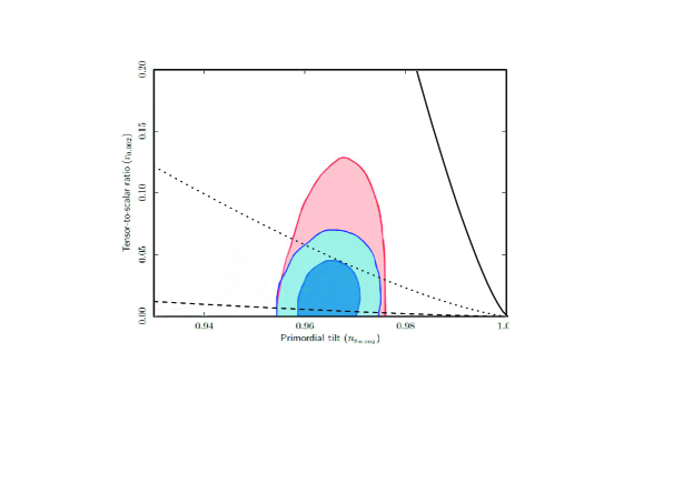
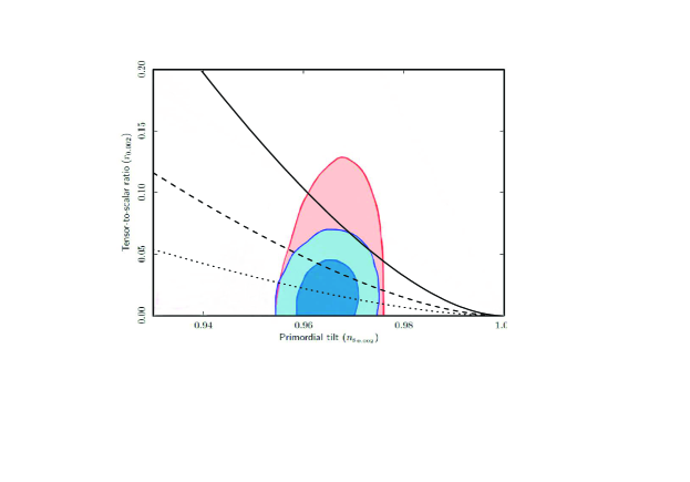
Figure 1: The upper and lower panels show the tensor-to-scalar ratio $r$ as a function of the scalar spectral index $n_{s}$, for three different values of the brane tension $\tau$. In both panels we have considered the two-marginalized constraints jointly as 68$\%$ and 95$\%$ C.L. at $k=0.002$ Mpc^-1 from the Planck 2018 results Planck2018 . Also, in both panels the solid, dashed and dotted lines correspond to the values of brane tension $\tau/m_{p}^{4}=10^{-12},10^{-13}$ and $10^{-14}$, respectively. In the upper panel we show the consistency relation for the specific case in which the constant $\beta=0$ and we have used $\alpha=10^{38}m_{p}^{-12}$. In the lower panel we show the case in which $\beta\neq 0$ and we have considered $\beta=\alpha/60$ and $\alpha=3\times 10^{9}(\kappa/\tau)^{2}$, respectively.

On the other hand, in the reconstruction for the situation in which the constant of integration $\beta\neq 0$, we find that considering Eq.(31) the relation between $dN$ and $d\phi$ can be written as

$$\frac{dN}{[\alpha N^{2}+\beta N^{3}]^{1/3}}=\frac{dN}{\beta^{1/3}[\alpha_{0}N^{2}+N^{3}]^{1/3}}=C_{1}d\phi,\,\,\,\,\;\>\;\mbox{where}\,\,\,\,\,\;\;\;C_{1}=3^{1/3}\left(\frac{\kappa}{2\alpha\tau}\right)^{1/2},$$ (41)

and the quantity $\alpha_{0}=\alpha/\beta$. In the following, we will consider for simplicity the case in which the constant of integration $\beta>0$ i.e, $\alpha_{0}>0$. We also note that the integration of Eq.(41) does not permit one to obtain an analytical solution for the number of $e$-folds as a function of the scalar field i.e., $N=N(\phi)$. In this sense, the solution of Eq.(41) can be written as

$$\sqrt{3}\arctan\left[\left(1+2\left[1+\frac{\alpha_{0}}{N}\right]^{-1/3}\right)/\sqrt{3}\right]+\frac{1}{2}\ln\left[1+\left(1+\frac{\alpha_{0}}{N}\right)^{-2/3}+\left(1+\frac{\alpha_{0}}{N}\right)^{-1/3}\right]$$

$$-\ln\left[1-\left(1+\frac{\alpha_{0}}{N}\right)^{-1/3}\right]=\beta^{1/3}\,C_{1}\,(\phi-\phi_{0}),$$ (42)

where $\phi_{0}$ denotes a constant of integration.

Numerically, we note that in the limit in which $\alpha/\beta=\alpha_{0}<N$, the first two terms of Eq.(42) are approximately constants and the dominant term corresponds to (see Fig.2 )

$$-\ln\left[1-\left(1+\frac{\alpha_{0}}{N}\right)^{-1/3}\right]\approx\beta^{1/3}\,C_{1}\,(\phi-\phi_{0}).$$ (43)

Thus, we find that the reconstruction of the effective potential $V(\phi)$ considering the specific case in which $\alpha_{0}<N$ is given by

$$V(\phi)\approx\frac{1}{(3\,\beta)^{1/3}}\,\,\left[1-\exp(-\beta^{1/3}\,C_{1}\,[\phi-\phi_{0}])\right].$$ (44)

Here, we have combined Eqs.(34) and (43). Curiously, we observe that this effective potential is similar to that obtained in the Starobinsky model Staro in which $\beta^{1/3}\,C_{1}=\sqrt{2/3}\,m_{p}^{-1}$ i.e., $\beta^{1/3}\,C_{1}\,m_{p}\approx\mathcal{O}(1)$. Also, in the limit $\beta^{1/3}\,C_{1}\,[\phi-\phi_{0}]\gg 1$, the effective potential corresponds to a constant potential i.e., a solution of de Sitter.

For the inverse case in which $\alpha_{0}>N$, we note that the first term of Eq.(42) dominates with which (see Fig.2 )

$$\sqrt{3}\arctan\left[\left(1+2\left[1+\frac{\alpha_{0}}{N}\right]^{-1/3}\right)/\sqrt{3}\right]\approx\beta^{1/3}\,C_{1}\,(\phi-\phi_{0}).$$ (45)

In this form, we obtain that the reconstruction in the limit in which $\alpha_{0}>N$ becomes

$$V(\phi)\approx\frac{1}{2(3\beta)^{1/3}}\left[\sqrt{3}\tan(\beta^{1/3}C_{1}(\phi-\phi_{0})/\sqrt{3})-1\right].$$ (46)

Here the range for the scalar field is given by $\frac{\sqrt{3}\,\pi}{6\beta^{1/3}C_{1}}+\phi_{0}\lesssim\phi\lesssim\frac{\sqrt{3}\,\pi}{2\beta^{1/3}C_{1}}+\phi_{0}$.

Figure 2: Evolution of the three terms on the right given by Eq.(42) versus the dimensionless quantity $\frac{\alpha}{\beta\,N}=\frac{\alpha_{0}}{N}$. Here, the dotted, dashed, and solid lines denote the first, second and third terms of Eq.(42), respectively.

In Fig.1 we show the ratio $r$ versus the spectral index $n_{s}$, for three different values of the brane tension $\tau$. In both panels we consider the two-marginalized constraints for the consistency relation $r=r(n_{s})$ (at 68$\%$ and 95$\%$ CL at $k=0.002$ Mpc^-1 ) from the new Planck data Planck2018 . In the upper panel we consider the special case in which the constant of integration $\beta=0$, where the consistency relation is given by Eq.(38). Here, we take the value $\alpha=10^{38}m_{p}^{-12}$. In the lower panel we take into account the case in which $\beta\neq 0$ and for the relation $r=r(n_{s})$ we have used Eq.(38). In this case we have considered the specific value of $\beta$ at $N=60$ (point limit $\alpha_{0}/N=1$ or $\beta=\alpha/N$) wherewith $\beta=\alpha/60$ and $\alpha=3\times 10^{9}(\kappa/\tau)^{2}$, respectively. Also, in both panels the solid, dashed and dotted lines correspond to the values of brane tension $\tau/m_{p}^{4}=10^{-12},10^{-13}$ and $10^{-14}$, respectively. In particular for the case $\beta=0$ we find that the brane tension has an upper limit given by $\tau<10^{-13}m_{p}$, as can be seen of the upper panel of Fig.1. For the case in which $\beta\neq 0$ we find that in the particular case in which $\beta=\alpha/60$, the value of the brane tension $\tau<10^{-12}m_{p}^{4}$ is well corroborated by Planck 2018 results, see lower panel of Fig.1. This suggests that the value of the constant of integration $\beta$ modifies the the upper bound on the brane tension. We note that in the case in which the constant $\beta>\alpha/60$ the upper limit on the brane tension increases and in the opposite case ($\beta<\alpha/60$ ) the upper limit on $\tau$ decreases.

In Fig.2 we show the behavior of the three terms on the right of Eq.(42) versus the dimensionless quantity $\frac{\alpha}{\beta\,N}=\frac{\alpha_{0}}{N}$. We note that for the limit in which $\alpha_{0}<N$ dominates the third term of Eq.(42), see solid line of Fig.2. However, for the case in which $\alpha_{0}>N$ the dominant term corresponds to the first expression of Eq.(42) given by dotted line in Fig.2.

In order to clarify our above results, we can study some specific limits for the ratio $\alpha/(\beta N)=\alpha_{0}/N$ in which $\alpha_{0}/N\ll 1$ and $\alpha_{0}/N\gg 1$. As a first approximation we consider the case in which $\alpha_{0}/N\ll 1$ or $\alpha_{0}\ll N$. For this limit we find from Eq.(41) that the relation $N=N(\phi)$ is given by

$$N(\phi)=\exp[\beta^{1/3}\,C_{1}\,(\phi-\phi_{0})],$$ (47)

where $\phi_{0}$ denotes a constant of integration. Thus, considering the limit $\alpha/(\beta)=\alpha_{0}\ll N$ we obtain that the effective potential $V(\phi)$ given by Eq.(34) becomes a constant and equal to $V(\phi)=(3\beta)^{-1/3}$. In fact, this result indicates an accelerated expansion de Sitter or de Sitter inflation, since in the high energy limit and considering the slow-roll approximation, we have $H\propto V=$constant. Note that this constant potential coincides with the potential given by Eq.(44) when $\beta^{1/3}\,C_{1}\,[\phi-\phi_{0}]\gg 1$. We also observe that for the consistency relation $r=r(n_{s})$, we get $r=48\tau\alpha/[(3\beta)^{2/3}N^{2}]\propto(1-n_{s})^{2}$ (see Eq.(38)).

For the case in which $\alpha/(\beta N)\gg 1$ or $\alpha_{0}\gg N$, we find from Eq.(41) that the relation $N=N(\phi)$ coincides with the case $\beta=0$ i.e., Eq.(39) and then the effective potential $V(\phi)$ changes linearly with the scalar field according to Eq.(40) in which $V(\phi)\propto\phi$. This effective potential agrees with the potential given by Eq.(46) assuming that the argument $\beta^{1/3}C_{1}(\phi-\phi_{0})/\sqrt{3}<1.$

V High energy:Reconstruction from the attractor $r(N)$

In this section we consider the hight energy limit, in order to reconstruct the effective potential $V(\phi)$, but from a different point of view. In order to reconstruct the scalar potential, we consider as an attractor the tensor to scalar ratio in terms of the number of $e-$foldings $N$ i.e., $r=r(N)$. In this sense, considering Eq.(32) we obtain that the potential effective $V(N)$ can be written as

$$V=V(N)=-48\tau\,\left[\int\,r\,dN\right]^{-1}.$$ (48)

Now from Eq.(27) we find that the relation between the number $N$ and the scalar field $\phi$ is given by

$$r^{1/2}\,\frac{dN}{d\phi}=(24\kappa)^{1/2}.$$ (49)

Here, we have considered Eq.(32).

In this context, we can obtain the scalar spectral index $n_{s}$ as a function of the number of $e$-folds $N$, combining the expressions given by Eqs.(29) and (48) for a specific attractor $r=r(N)$. Thus, the scalar spectral index can be rewritten as

$$n_{s}-1=\,\left[\ln\left(\frac{r}{48\tau V^{2}}\right)\right]_{,\,N}.$$ (50)

Here, the potential $V$ is given by Eq.(48).

V.1 An example of $r=r(N)$.

In order to develop the reconstruction of the scalar potential $V(\phi)$ in the brane world inflation, we consider that the attractor for the tensor to scalar ratio as a function of the number of $e$- folds $r(N)$ is given by

$$r(N)=\frac{\alpha_{1}}{N^{2}},$$ (51)

where $\alpha_{1}>0$ corresponds to a constant (dimensionless). For this attractor the cases in which $\alpha_{1}=12$, was analyzed in Ref.T , and the specific value $\alpha_{1}=8$, was obtained in Ref. Chiba:2015zpa .

In particular considering $N=60$ and $r<0.07$, we find that the value of the constant $\alpha_{1}<252$.

By combining Eqs.(48) and (51) we obtain that the scalar potential in terms of the number of $e$-foldings becomes

$$V(N)=\frac{1}{\alpha_{2}/N+\beta_{1}},\,\,\,\,\,\,\,\mbox{where}\,\,\,\,\,\,\alpha_{2}=\frac{\alpha_{1}}{48\tau}.$$ (52)

Here the quantity $\beta_{1}$ corresponds to a constant of integration with units of $m_{p}^{-4}$.

In order to obtain the relation between the number $N$ and the scalar field $\phi$, we consider Eq.(49) together with the attractor given by Eq.(51) obtaining

$$N=\exp\left[\sqrt{\frac{24\kappa}{\alpha_{1}}}\,(\phi-\phi_{0})\right],$$ (53)

where $\phi_{0}$ denotes a new constant of integration. Thus, the reconstruction of the scalar potential in terms of the scalar field can be written as

$$V(\phi)=\left(\alpha_{2}\,\exp\left[-\sqrt{\frac{24\kappa}{\alpha_{1}}}\,(\phi-\phi_{0})\right]+\beta_{1}\right)^{-1}.$$ (54)

In particular assuming that $\beta_{1}>0$ and $\alpha_{2}/\beta_{1}\gg N$, the effective potential has the behavior of an exponential potential i.e., $V(\phi)\propto e^{(\sqrt{24\kappa/\alpha_{1}}\,)\,\phi}$ (recall the we have considered that $V^{\prime}>0$). In the inverse case in which $N\gg\alpha_{2}/\beta_{1}$, the scalar potential corresponds to a constant potential $V(\phi)=$ constant.

In the context of the cosmological perturbations, we find in the high energy limit the power spectrum becomes

$${\mathcal{P}_{\mathcal{R}}}\simeq\frac{1}{12\pi^{2}}\,\left(\frac{\kappa V^{2}}{2\tau}\right)^{3}\,\frac{1}{V^{\prime}\,{}^{2}}=\frac{\kappa^{2}}{48\pi^{2}\tau^{2}}\,\left(\frac{V^{4}}{V_{,\,N}}\right)=\frac{\kappa^{2}}{48\pi^{2}\tau^{2}}\,\frac{N^{2}}{\alpha_{2}}\,\left(\frac{\alpha_{2}}{N}+\beta_{1}\right)^{-2}.$$ (55)

Here we have used Eqs.(11) and (52), respectively. Thus, we can write the constant $\beta_{1}$ in terms of the scalar spectrum ${\mathcal{P}_{\mathcal{R}}}$, the number of $e$-folds $N$ and the constant $\alpha_{2}$ as

$$\beta_{1}=\sqrt{\frac{1}{3\,\alpha_{2}\,{\mathcal{P}_{\mathcal{R}}}}}\,\left(\frac{\kappa\,N}{4\pi\,\tau}\right)-\frac{\alpha_{2}}{N}=\sqrt{\frac{\alpha_{2}}{3\,\,{\mathcal{P}_{\mathcal{R}}}}}\,\left(\frac{12\kappa\,N}{\pi\,\alpha_{1}}\right)-\frac{\alpha_{2}}{N}.$$ (56)

On the other hand, from Eq.(50) we find that the relation between the scalar index $n_{s}$ and the number of $e$-foldings is given by

$$n_{s}-1=\frac{2}{N}\left[\frac{\beta_{1}}{\alpha_{2}/N+\beta_{1}}-2\right].$$ (57)

Note that in the specific case in which $N\gg\alpha_{2}/\beta_{1}$, the scalar spectral index $n_{s}$ gives the famous attractor $n_{s}-1=-2/N$.

Now, from Eq.(57) we can find the constant $\beta_{1}$ in terms of $n_{s}$, $N$ and $\alpha_{2}$ as

$$\beta_{1}=\frac{[N(n_{s}-1)+4]}{N[(1-n_{s})N-2]}\,\alpha_{2}.$$ (58)

Note that for the values $n_{s}=0.964$ and $N=60$, we have that the ratio $\alpha_{2}/\beta_{1}\sim 5$. This suggests that the limit $\alpha_{2}/\beta\gg N$ is not satisfied for large $N$, then the exponential potential $V(\phi)\propto e^{\phi}$ does not work in the braneworld. This analysis for the exponential potential in the framework of a brane coincides with that obtained in Ref.Tsujikawa:2003zd . Thus, the reconstruction of the effective potential $V(\phi)$ is given by Eq.(54) for large $N$ and an appropriate limit corresponds to $N\gg\alpha_{2}/\beta_{1}$, where the behavior of the scalar potential becomes constant.

In this form, combining Eqs.(56) and (58) we find that the tension $\tau$ as function of the observables $n_{s}$ and ${\mathcal{P}_{\mathcal{R}}}$ together with the number of $e$-foldings $N$ and $\alpha_{1}$ becomes

$$\tau=\left(\frac{{\mathcal{P}_{\mathcal{R}}}\;\pi^{2}\,\alpha_{1}^{3}}{4\,\times 12^{3}\,\kappa^{2}\,N^{4}}\right)\,\,\left[\frac{[N(n_{s}-1)+4]}{[(1-n_{s})N-2]}+1\right]^{2}.$$ (59)

Here we have used that $\alpha_{2}=\alpha_{1}/(48\tau)$.

In particular assuming that the spectral index $n_{s}=0.964$, the spectrum ${\mathcal{P}_{\mathcal{R}}}\simeq 2.2\times 10^{-9}$ and $N=60$, we obtain that the constraint on the brane tension $\tau$ is given by

$$\tau\simeq\,6\times 10^{-20}\,\alpha_{1}^{3}\,\,m_{p}^{4}.$$ (60)

Note that Eq.(60) gives a relation between the brane tension and the parameter $\alpha_{1}$. Now, by assuming that $\alpha_{1}<252$ in order to obtain $r<0.07$ at $N=60$, we find that the upper bound for the brane tension becomes

$$\tau<9.6\times 10^{-13}\,m_{p}^{4}\simeq 10^{-12}\,m_{p}^{4}.$$

On the other hand, from Eq.(57) we find that the relation between the scalar index and the tensor to scalar ratio, can be written as

$$n_{s}-1=-\frac{2\,r^{1/2}}{\alpha_{1}^{1/2}}\,\left[\frac{2\alpha_{2}+\beta_{1}\sqrt{\alpha_{1}/r}}{\alpha_{2}+\beta_{1}\sqrt{\alpha_{1}/r}}\right].$$ (61)

Here we have used the attractor given by Eq.(51).

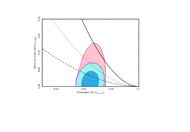
Figure 3: As before, we show the tensor-to-scalar ratio $r$ as a function of the scalar spectral index $n_{s}$ from Planck 2018 resultsPlanck2018 for three different values of the brane tension $\tau$ but assuming the attractor $r(N)\propto N^{-2}$ as the starting point. Solid, dotted and dashed lines correspond to the values of brane tension $\tau/m_{p}^{4}=10^{-11},10^{-12}$ and $10^{-13}$, respectively.

In Fig.3 we show the tensor to scalar ratio versus the scalar spectral index for three different values of the brane tension considering the attractor $r(N)=\alpha_{1}\,N^{-2}$. Here we have used Eq.(61) and the solid, dotted and dashed lines correspond to the values of brane tension $\tau/m_{p}^{4}=10^{-11},10^{-12}$ and $10^{-13}$, respectively. From this plot we check that the upper limit for the brane tension given by $\tau<10^{-12}m_{p}^{4}$ is well corroborated from Planck data.

VI Conclusions

In this article we have analyzed the reconstruction of the background in the context of braneworld inflation. Considering a general formalism of reconstruction, we have obtained an expression for the effective potential under the slow roll approximation. In order to obtain analytical solutions in the reconstruction on the brane, we have considered the high energy limit in which the energy density $\rho\simeq V\gg\tau$. In this analysis for the reconstruction of the background, we have considered the parametrization of the scalar spectral index or the tensor to scalar ratio as function of the number of $e$-foldings $N$. In this general description we have found from the cosmological parameter $n_{s}(N)$ or the parameter $r(N)$, integrable solutions for the effective potential depending on the cosmological attractor $n_{s}(N)$ or $r(N)$.

For the reconstruction from the attractor associated with scalar spectral index $n_{s}(N)$, we have assumed the famous attractor $n_{s}=1-2/N$ as an example. From this attractor, we have obtained that the consistency relation $r=r(n_{s})$ is given by Eq.(38) and from the power spectrum we have found that the integration constant $\alpha$ depends on the brane tensor, see Eq.(36). On the other hand, depending on the value of the second constant of integration $\beta$, we have found different results for the reconstruction of the effective potential $V(\phi)$. In particular for the specific case in which the constant $\beta=0$, we have obtained that the reconstruction of the effective potential corresponds to a potential $V(\phi)\propto\,\phi$. Also, assuming that the observational constraint on the tensor to scalar ratio $r<0.07$, we have found an upper limit for the brane tension given by $\tau<10^{-13}m_{p}^{4}$, wherewith the brane model is well supported by the Planck data, see upper panel of Fig.1. In this same context, for the case in which the constant of integration $\beta\neq 0$, we have found a transcendental equation for the number of $e$-folds as a function of the scalar field $N=N(\phi)$ and the reconstruction does not work. However, as a first approximation we have analyzed the dominant terms of the transcendental equation in order to give an approach to the reconstruction of the effective potential; see Fig.2. Also, we have considered the extreme limits $\alpha_{0}/N\ll 1$ and $\alpha_{0}/N\gg 1$, in order to find analytical expressions for the potential $V(\phi)$. In this approach, we have obtained that in the limit in which $\alpha_{0}/N\gg 1$, the effective potential coincides with the case in which the constant of integration $\beta=0$, where the effective potential changes linearly with the scalar field.

On the other hand, we have explored the possibility of the reconstruction in the framework of braneworld inflation, considering as an attractor the tensor to scalar ratio in terms of the number of $e$-foldings i.e., $r=r(N)$. Here we have found general relation in order to build the effective potential. As a specific example, we have considered the attractor $r(N)\propto N^{-2}$. Here, we have obtained that the reconstruction of the effective potential is given by Eq.(54). In particular, considering the limit in which $\alpha_{2}/\beta_{1}\gg N$, we have obtained that the effective potential corresponds to an exponential potential i.e., $V(\phi)\propto e^{\phi}$; however this limit does not work. In the inverse limit, we have found that the effective potential $V(\phi)=$ constant. Also, utilizing the observables as the scalar spectral index and the power spectrum together with the number of $e$-folds, we have found a relation between the brane tension and the associated parameter $\alpha_{1}$ to the attractor $r(N)$. Thus, by considering that $\alpha_{1}<252$, in order to obtain $r<0.07$ at $N=60$, we have found an upper bound on the brane tension given by $\tau<10^{-12}m_{p}^{4}$ and this constraint is well corroborated with Planck data, see Fig.3.

We have also found that in the framework of braneworld inflation, the incorporation of the additional term in Friedmann’s equation affects substantially the reconstruction of the effective potential $V(\phi)$, considering the simplest attractors, such as $n_{s}(N)-1\propto N^{-1}$ or $r(N)\propto N^{-2}$. In this respect, we have shown that in order to obtain analytical solutions for the reconstruction of $V(\phi)$, the attractor $r(N)$, is an adequate methodology to be considered.

We conclude with some comments concerning the way to distinguish the reconstruction in the braneworld and GR inflationary models from the methodology used. For the famous attractor $n_{s}-1=-2/N$, we have found that the reconstruction from $n_{s}(N)$ in braneworld inflation does not work unlike in GR. Here, we have shown that for a specific case in which the integration constants is zero, the reconstruction from $n_{s}(N)$ works. On the other hand, by assuming the reconstruction of braneworld inflation from the attractor $r(N)$, we have been able to rebuild our model as it occurs in the framework of GR. This suggests that the version of reconstruction from $r(N)$ is a suitable ansatz to be used for the reconstruction of braneworld inflation.

Finally, in this paper we have not addressed the reconstruction of the braneworld model as a fluid, considering an ansatz on the effective EoS as a function of the number of $e-$folds. We hope to return to this methodology in the near future.

- (1) A.A. Starobinsky, Phys. Lett. B 91, 99 (1980).
- (2) A. Guth, Phys. Rev. D 23, 347 (1981).
- (3) A. Albrecht and P. J. Steinhardt, Phys. Rev. Lett. 48, 1220 (1982); A complete description of inflationary scenarios can be found in the book by A. Linde , Particle physics and inflationary cosmology (Gordon and Breach, New York, 1990).
- (4) A. Guth and S.-Y. Pi, Phys. Rev. Lett. 49, 1110 (1982); S. W. Hawking, Phys. Lett. 115 B, 295 (1982).
- (5) D. Larson et al., Astrophys. J. Suppl. 192, 16 (2011).
- (6) C. L. Bennett et al., Astrophys. J. Suppl. 192, 17 (2011); N. Jarosik et al., Astrophys. J. Suppl. 192, 14 (2011).
- (7) Y. Akrami et al. [Planck Collaboration], arXiv:1807.06211 [astro-ph.CO].
- (8) A. Sen, JHEP 0204, 048 (2002).
- (9) K. Akama, Lect. Notes Phys. 176, 267 (1982); V. A. Rubakov and M. E. Shaposhnikov, Phys. Lett. B 159, 22 (1985); N. Arkani Hamed, S. Dimopoulos, and G. Dvali, Phys. Lett. B 429, 263 (1998); M. Gogberashvili, Europhys. Lett. 49, 396 (2000); L. Randall and R. Sundrum, Phys. Rev. Lett. 83, 3370 (1999); 83, 4690 (1999).
- (10) T. Shiromizu, K. Maeda, and M. Sasaki, Phys. Rev. D 62, 024012 (2000).
- (11) P. Binetruy, C. Deffayet, and D. Langlois, Nucl. Phys. B565, 269 (2000); P. Binetruy, C. Deffayet, U. Ellwanger, and D. Langlois, Phys. Lett. B 477, 285 (2000).
- (12) L. Randall and R. Sundrum, Phys.Rev.Lett.83, 4690 (1999).
- (13) R. Maartens, D. Wands, B. A. Bassett and I. Heard, Phys. Rev. D 62, 041301 (2000).
- (14) G. Huey and J. E. Lidsey, Phys. Lett. B 514, 217 (2001).
- (15) M. Sami, Mod. Phys. Lett. A 18, 691 (2003).
- (16) R. Maartens, D. Wands, B. A. Bassett, and I. P. C. Heard, Phys. Rev. D 62, 041301 (2000).
- (17) J. M. Cline, C. Grojean, and G. Servant, Phys. Rev. Lett.83, 4245 (1999); C. Csaki, M. Graesser, C. F. Kolda and J. Terning, Phys. Lett. B 462 34 (1999); D. Ida, JHEP 0009, 014 (2000); R. N. Mohapatra, A. Perez-Lorenzana, and C. A. de S. Pires, Phys. Rev. D 62, 105030 (2000); R. N. Mohapatra, A. Perez-Lorenzana, and C. A. de S. Pires, Int. J. Mod. Phys. A 16, 1431 (2001); S. del Campo, R. Herrera and J. Saavedra, Phys. Rev. D 70, 023507 (2004); C. Campuzano, S. del Campo, R. Herrera and R. Herrera, Phys. Rev. D 72, 083515 (2005); Y. Gong, arXiv:gr-qc/0005075; B. A. Bassett, S. Tsujikawa and D. Wands, Rev. Mod. Phys. 78, 537 (2006); M. A. Cid, S. del Campo and R. Herrera, JCAP 0710, 005 (2007); R. Herrera, Phys. Lett. B 664, 149 (2008); S. del Campo and R. Herrera, Phys. Lett. B 670, 266 (2009); R. Herrera, Gen. Rel. Grav. 41, 1259 (2009); Y. Ling and J. P. Wu, JCAP 1008, 017 (2010); K. C. Wong, K. S. Cheng and T. Harko, Eur. Phys. J. C 68, 241 (2010); R. Herrera and N. Videla, Eur. Phys. J. C 67, 499 (2010); R. Herrera and E. San Martin, Eur. Phys. J. C 71, 1701 (2011)
- (18) R. Maartens, doi:10.1142/9789812810021-0008 gr-qc/0101059; M. Bouhmadi-Lopez, P. Chen, Y. -W. Liu, P. Chen and Y. -W. Liu, Phys. Rev. D 86, 083531 (2012); R. Herrera, M. Olivares and N. Videla, Eur. Phys. J. C 73, no. 6, 2475 (2013); R. Herrera, N. Videla and M. Olivares, Eur. Phys. J. C 75, no. 5, 205 (2015).
- (19) R. Kallosh, A. Linde and Y. Yamada, JHEP 1901, 008 (2019); C. M. Lin, K. W. Ng and K. Cheung, arXiv:1810.01644 [hep-ph]; R. Y. Guo, L. Zhang, J. F. Zhang and X. Zhang, Sci. China Phys. Mech. Astron. 62, no. 3, 30411 (2019); M. R. Gangopadhyay and G. J. Mathews, JCAP 1803, no. 03, 028 (2018); N. Jaman and K. Myrzakulov, arXiv:1807.07443 [gr-qc]; I. Banerjee, S. Chakraborty and S. SenGupta, Phys. Rev. D 99, no. 2, 023515 (2019).
- (20) H. M. Hodges and G. R. Blumenthal, Phys. Rev. D 42, 3329 (1990).
- (21) R. Easther, Class. Quantum Grav. 13, 1775 (1996).
- (22) J. Martin, D. Schwarz, Phys. Lett. B 500, 1-7 (2001).
- (23) X. z. Li and X. h. Zhai, Phys. Rev. D 67, 067501 (2003).
- (24) R. Herrera and R. G. Perez, Phys. Rev. D 93, no. 6, 063516 (2016).
- (25) T. Chiba, PTEP 2015, no. 7, 073E02 (2015).
- (26) T. Miranda, J. C. Fabris and O. F. Piattella, JCAP 1709, no. 09, 041 (2017); A. Achúcarro, R. Kallosh, A. Linde, D. G. Wang and Y. Welling, JCAP 1804, no. 04, 028 (2018).
- (27) R. Kallosh and A. Linde, JCAP 1307, 002 (2013).
- (28) R. Kallosh and A. Linde, JCAP 1310, 033 (2013).
- (29) A. D. Linde, Phys. Lett. B 129, 177, (1983).
- (30) D. Kaiser, Phys. Rev. D 52, 4295-4306 (1995); F Bezrukov and M. Shaposhnikov, Phys Lett B 659, 703, (2008).
- (31) R. Kallosh, A. Linde, D. Roest, Phys Rev Lett, 112 011303, (2014).
- (32) R. Herrera, Eur. Phys. J. C 78, no. 3, 245 (2018).
- (33) R. Herrera, Phys. Rev. D 98, no. 2, 023542 (2018).
- (34) Q. G. Huang, Phys. Rev. D 76, 061303 (2007).
- (35) J. Lin, Q. Gao and Y. Gong, Mon. Not. Roy. Astron. Soc. 459, no. 4, 4029 (2016); Q. Gao, Sci. China Phys. Mech. Astron. 60, no. 9, 090411 (2017).
- (36) D. Roest, JCAP 1401, 007 (2014).
- (37) J. Garcia-Bellido and D. Roest, Phys. Rev. D 89, no. 10, 103527 (2014).
- (38) P. Creminelli, S. Dubovsky, D. López Nacir, M. Simonovic, G. Trevisan, G. Villadoro and M. Zaldarriaga, Phys. Rev. D 92, no. 12, 123528 (2015).
- (39) S. D. Odintsov and V. K. Oikonomou, Phys. Rev. D 98, no. 4, 044039 (2018).
- (40) S. D. Odintsov and V. K. Oikonomou, Annals Phys. 388, 267 (2018).
- (41) S. D. Odintsov and V. K. Oikonomou, Nucl. Phys. B 929, 79 (2018); B. Tajahmad, arXiv:1812.10339 [gr-qc]; M. Rinaldi, G. Cognola, L. Vanzo and S. Zerbini, JCAP 1408 (2014);K. Bamba, S. Nojiri and S. D. Odintsov, Phys. Lett. B 737, 374 (2014).
- (42) V. Mukhanov, Eur. Phys. J. C 73, 2486 (2013); V. Mukhanov, Fortsch. Phys. 63, 36 (2015).
- (43) R. Myrzakulov and L. Sebastiani, Astrophys. Space Sci. 356, no. 1, 205 (2015); R. Myrzakulov and L. Sebastiani, Astrophys. Space Sci. 357, no. 1, 5 (2015); R. Myrzakulov, L. Sebastiani and S. Zerbini, Eur. Phys. J. C 75, no. 5, 215 (2015); S. Myrzakul, R. Myrzakulov and L. Sebastiani, Astrophys. Space Sci. 357, no. 2, 168 (2015).
- (44) R. Myrzakulov and L. Sebastiani, Astrophys. Space Sci. 357, no. 1, 5 (2015).
- (45) S. Capozziello; V. F. Cardone; E. Elizalde; S. Nojiri; S. D. Odintsov, Phys. Rev. D 73, 043512:1–043512:16 (2006); S. Nojiri and S. D. Odintsov, Phys. Rev. D 72, 023003 (2005); S. Nojiri and S. D. Odintsov, Phys. Lett. B 639, 144 (2006); K. Bamba, S. Capozziello, S. Nojiri and S. D. Odintsov, Astrophys. Space Sci. 342, 155 (2012); I. H. Brevik and O. Gorbunova, Gen.Rel.Grav. 37 2039-2045 (2005); I. H. Brevik and O. Gorbunova, Eur. Phys. J. C 56, 425 (2008).
- (46) S. Capozziello, V. F. Cardone, E. Elizalde, S. Nojiri and S. D. Odintsov, Phys. Rev. D 73, 043512 (2006); I. Brevik, O. Gron, J. de Haro, S. D. Odintsov and E. N. Saridakis, Int. J. Mod. Phys. D 26, no. 14, 1730024 (2017).
- (47) F. Lucchin, S. Matarrese, Phys. Rev. D 32, 1316 (1985);
- (48) J. D. Barrow, Phys. Lett. B 235, 40 (1990).
- (49) J. D. Barrow and N. J. Nunes, Phys. Rev. D 76, 043501 (2007).
- (50) R. Herrera, N. Videla and M. Olivares, Eur. Phys. J. C 78, no. 11, 934 (2018).
- (51) S. Nojiri and S. D. Odintsov, J. Phys. Conf. Ser. 66, 012005 (2007); K. Bamba, S. Capozziello, S. Nojiri and S. D. Odintsov, Astrophys. Space Sci. 342, 155 (2012); A. Jawad and S. Rani, Astrophys. Space Sci. 357, no. 1, 88 (2015).
- (52) G. Sethi, A. Dev and D. Jain, Phys. Lett. B 624, 135 (2005); N. Goheer, J. Larena and P. K. S. Dunsby, Phys. Rev. D 80, 061301 (2009); E. Elizalde, E.O. Pozdeeva, and S.Yu. Vernov, Phys. Rev. D 85, 044002 (2012); S.Yu. Vernov, Phys. Part. Nucl. 43 694–696 (2012); A. Y. Kamenshchik, A. Tronconi, G. Venturi and S. Y. Vernov, Phys. Rev. D 87, no. 6, 063503 (2013);
- (53) A. Kamenshchik, U. Moschella and V. Pasquier, Phys. Lett. B 511, 265 (2001); N. Bilic, G. B. Tupper and R. D. Viollier, Phys. Lett. B 535, 17 (2002).
- (54) R. Maartens, doi:10.1142/9789812810021-0008 gr-qc/0101059.
- (55) P. Bowcock, C. Charmousis and R. Gregory, Class. Quant. Grav. 17, 4745 (2000).
- (56) J. M. Cline, C. Grojean and G. Servant, Phys. Rev. Lett. 83, 4245 (1999).
- (57) P. Brax and C. van de Bruck, Class. Quant. Grav. 20, R201 (2003).
- (58) T. Clifton, P. G. Ferreira, A. Padilla and C. Skordis, Phys. Rept. 513, 1 (2012).
- (59) D. Langlois, R. Maartens and D. Wands, Phys. Lett. B 489, 259 (2000).
- (60) S. Tsujikawa and A. R. Liddle, JCAP 0403, 001 (2004); E. J. Copeland and O. Seto, Phys. Rev. D 72, 023506 (2005).