Infinite square-well, trigonometric Pöschl-Teller and other potential wells with a moving barrier

Abstract

Using mainly two techniques, a point transformation and a time dependent supersymmetry, we construct in sequence several quantum infinite potential wells with a moving barrier. We depart from the well known system of a one-dimensional particle in a box. With a point transformation, an infinite square-well potential with a moving barrier is generated. Using time dependent supersymmetry, the latter leads to a trigonometric Pöschl-Teller potential with a moving barrier. Finally, a confluent time dependent supersymmetry transformation is implemented to generate new infinite potential wells, all of them with a moving barrier. For all systems, solutions of the corresponding time dependent Schrödinger equation fulfilling boundary conditions are presented in a closed form.

1 Introduction

There are physical problems where the boundary conditions of the underlying equation can move. Examples of them are the so called Stefan problems, where temperature as a function of position and time on a system of water and ice has to be found, the interface water-ice imposes a boundary condition that changes its position with time [1]. Another example was drafted by Fermi, he theorized the origin of cosmic radiation as particles accelerated by collisions with a moving magnetic field [2], this problem was later studied by Ulam [3] in a classical framework where the statistical properties of particles in a box with oscillating infinite barriers were analyzed numerically. In this paper, we are interested in systems ruled by the time dependent Schrödinger equation. In particular, we show how different quantum systems with a moving boundary condition and their solutions can be generated using basically two tools, a point transformation and a time dependent supersymmetry.

The point transformation we use was introduced in [4, 5] where the authors mapped solutions between two time dependent Schrödinger equations with different potentials. This transformation can be used, for example, to map solutions of the harmonic oscillator to solutions of the free particle system.

On the other hand, the supersymmetry technique or SUSY helps as well to map solutions between two Schrödinger equations, but in this case the potentials share properties like asymtotic behavior or a similiar discrete spectrum in case of time-independent potentials. A first version links two time independent one-dimensional Schrödinger equations [6, 7]. In this article we use the time dependent version, that links two time dependent Schrödinger equations [8, 9]. The involved potentials are referred as SUSY partners and if the link is made through a first-order differential operator, often called intertwining operator, the technique is known as 1-SUSY. Examples of time dependent SUSY partners of the harmonic oscillator can be found in [11, 10].

F. Finkel et.al. [12] showed that the time independent SUSY technique, and the time dependent version were related by the previously mentioned point transformation.

The structure of this article is as follows. The quantum particle in a box is revised in Sec. 2. In Sec. 3, we use a point transformation to generate an infinite square-well potential with a moving barrier. A brief review of time dependent SUSY is given in Sec. 4 and it is applied to the infinite square-well potential with a moving barrier to generate the exactly solvable system of a Pöschl-Teller potential with a moving barrier. In Sec. 5, we apply for the second time a supersymmetric transformation to the infinite square-well potential to obtain a biparametric family of infinite potential wells with a moving barrier. Exact solutions of the time dependent Schrödinger equation for each potential are given in the corresponding section. We finish this article with our conclusion.

2 Quantum infinite square-well potential

The quantum particle in a one-dimensional infinite square-well potential or particle in a box is a common example of an exact solvable model in textbooks, see for example [13, 14, 15]. It represents a particle trapped in the interval $0<y<L$ with impenetrable barriers, placed at zero and $L$, and inside that one-dimensional box the particle is free to move. The corresponding time independent Schrödinger equation is

$$\frac{d^{2}}{dy^{2}}\psi(y)+\frac{2m}{\hbar^{2}}\left(E-\widetilde{V}_{0}\right)\psi(y)=0,$$ (1)

where $E$ is a real parameter representing the energy of the particle, $m$ is its mass and $\hbar$ is Planck’s constant. Through this article we will use units where $m=1/2$ and $\hbar=1$. The one-dimensional infinite potential well $\widetilde{V}_{0}(y)$ is:

$$\widetilde{V}_{0}(y)=\left\{\begin{array}[]{cc}0,&\quad 0<y<L,\\ \infty,&\quad\text{otherwise},\end{array}\right.$$ (4)

where $L$ is a positive real constant. The solution of this eigenvalue problem is well known, eigenfunctions and eigenvalues are given by

$$\psi_{n}(y)=\sqrt{\frac{2}{L}}\sin\left(\frac{n\pi y}{L}\right),\qquad E_{n}=\left(\frac{n\pi}{L}\right)^{2},\qquad n=1,2,3,\dots.$$ (5)

Functions $\psi_{n}(y)$ satisfy the boundary conditions $\psi_{n}(0)=\psi_{n}(L)=0$. We will use this system to construct a variety of infinite potential wells where one of the barriers is moving.

3 From the particle in a box to the infinite square-well potential with a moving barrier

In this section we will use a point transformation in order to obtain from the stationary potential (4) an infinite square-well potential with a moving barrier. First we introduce a general point transformation [4, 5, 12, 16] and then we apply it on the particle in a box system. The simplified notation for the transformation was introduced in [16].

3.1 Point transformation

Consider a one dimension time independent Schrödinger equation in the spatial variable $y$ as

$$\frac{d^{2}}{dy^{2}}\psi(y)+\left(E-\widetilde{V}_{0}\right)\psi(y)=0$$ (6)

where $\widetilde{V}_{0}=\widetilde{V}_{0}(y)$ and a solution $\psi$ are known. Now let us take arbitrary functions $A=A(t)$ and $B=B(t)$ and let the variable $y$ be defined in terms of a temporal parameter $t$ and a new spatial variable $x$ as:

$$y(x,t)=x\exp\left[4\int A(t)dt\right]+2\int B(t)\exp\left[4\int A(t)dt\right]dt$$ (7)

then the function

$$\phi(x,t) = \psi(y(x,t))\exp\left\{-i\left[A(t)x^{2}+B(t)x+E\int\exp\left[8\int A(t)dt\right]dt\right.\right.$$ (8)

$$\left.\left.+\int\left[2iA(t)+B^{2}(t)\right]dt\right]\right\},$$

is solution of the equation

$$i\frac{\partial}{\partial t}\phi(x,t)+\frac{\partial^{2}}{\partial x^{2}}\phi(x,t)-V_{0}(x,t)\phi(x,t)=0.$$ (9)

The last equation is a time dependent Schrödinger equation where the potential is given by

$$V_{0}(x,t) = \widetilde{V}_{0}(y(x,t))\exp\left[8\int A(t)dt\right]+\left[\frac{d}{dt}A(t)-4A^{2}(t)\right]x^{2}$$ (10)

$$+\left[\frac{d}{dt}B(t)-4A(t)B(t)\right]x.$$

3.2 Infinite square-well potential with a moving barrier

We can use the point transformation to obtain an infinite square-well potential with a moving barrier. Without considering for this moment boundary conditions of the problem, we will transform the potential $\widetilde{V}_{0}(y)=0$ into $V_{0}(x,t)=0$. Apparently we are mapping a potential to itself but it will not be the case once we incorporate the boundary conditions. To make this transformation, functions $A(t)$ and $B(t)$ such that $V_{0}(x,t)=\widetilde{V}_{0}(y)=0$ in (10) need to be found. By setting $\widetilde{V}_{0}(y)=0$ and $V_{0}(x,t)=0$ in (10) we get

$$0 = \left[\frac{d}{dt}A(t)-4A^{2}(t)\right]x^{2}+\left[\frac{d}{dt}B(t)-4A(t)B(t)\right]x.$$ (11)

Coefficients of the previous polynomial in $x$ give us a system of coupled differential equations that can be solve:

$$\frac{d}{dt}A(t)-4A^{2}(t)=0, \quad\Rightarrow\quad A(t)=-\frac{1}{4t+c_{1}};$$

$$\frac{d}{dt}B(t)-4A(t)B(t)=0, \quad\Rightarrow\quad B(t)=\frac{c_{2}}{4t+c_{1}};$$ (12)

where $c_{1}$ and $c_{2}$ are real constants. Once these two functions are known, the change of variable defined in (7) can be evaluated,

$$y(x,t)=\frac{2x-c_{2}}{2(4t+c_{1})}.$$ (13)

At this point, we can discuss boundary conditions of the potential $V_{0}(x,t)$. The barriers of the potential (4) of the initial problem are located at $y_{1}=0$ and at $y_{2}=L$, using the change of variable (13) the new barriers will then be placed at $x_{1}=c_{2}/2$ and $x_{2}=4Lt+c_{1}L+c_{2}/2$, respectively. Thus, the potential $V_{0}(x,t)$ is

$$V_{0}(x,t)=\left\{\begin{array}[]{lll}0,&&x_{1}<x<\ell(t),\\ \infty,&&\text{otherwise},\end{array}\right.$$ (16)

where

$$\ell(t)=4Lt+c_{1}L+c_{2}/2.$$ (17)

This potential is an infinite square-well potential with a moving barrier. The meaning of the constants $c_{1}$ and $c_{2}$ can be extracted directly from the position of the boundaries of this potential. Indeed, the position of the fixed barrier is $c_{2}/2$, while the moving barrier is located at $\ell(t)$ and it is moving with a constant velocity $4L$. At $t_{0}=-c_{1}/4$ we have an ill defined problem (a particle in a box of length zero), so we should avoid this singularity, moreover, this time $t_{0}$ separates two problems: one of a contracting box and one where the potential well is expanding as time increases.

Finally, solutions of the time dependent Schrödinger equation (9) where $V_{0}(x,t)$ is (16) can be constructed using (5), (8), (12) and (13):

$$\phi_{n}(x,t) = \sqrt{\frac{2}{L(4t+c_{1})}}\sin\left\{\frac{n\pi}{L}\left[\frac{2x-c_{2}}{2(4t+c_{1})}\right]\right\}\exp\left[\frac{i}{4t+c_{1}}x^{2}-\frac{ic_{2}}{4t+c_{1}}x\right]$$ (18)

$$\times \exp\left[i\left(\frac{n\pi}{L}\right)^{2}\frac{1}{4(4t+c_{1})}+\frac{i~{}c_{2}^{2}}{4(4t+c_{1})}\right].$$

We will fix the constant $c_{2}=0$ so that one barrier is always at zero. We take as well $c_{1}=1$, then the moving barrier will be at $L$ when $t=0$. The singularity of the problem will be located at $t=-1/4$. For this selection of constant the functions $A$, $B$ in (12) and the change of variable $y$ in (13) simplify to

$$A(t)=-\frac{1}{4t+1},\quad B(t)=0,\quad y(x,t)=\frac{x}{4t+1};$$ (19)

the potential reads

$$V_{0}(x,t)=\left\{\begin{array}[]{lll}0,&&0<x<\ell(t),\quad\text{where}\quad\ell(t)=L(4t+1)\\ \infty,&&\text{otherwise},\end{array}\right.$$ (22)

and the solutions of the time dependent Schrödinger equation can be written as

$$\phi_{n}(x,t)=\sqrt{\frac{2}{\ell}}\sin\left(\frac{n\pi}{\ell}x\right)\exp\left\{i\frac{L}{\ell}\left[x^{2}+\left(\frac{n\pi}{2L}\right)^{2}\right]\right\}.$$ (23)

Note that $\phi_{n}(0,t)=\phi_{n}(\ell,t)=0$, satisfying the required boundary conditions of the physical problem. For this specific selection of the constants $c_{1}$ and $c_{2}$ the domain of the time variable for the contracting box is $(-\infty,-1/4)$ and for the expanding well is $(-1/4,\infty)$. Functions (23) are normalized $\int_{0}^{\ell}|\phi_{n}|^{2}dx=1$ at any given time. They form a complete orthogonal set at any fixed time and the expectation value of the energy $\langle E\rangle_{\phi_{n}}(t)=\int_{0}^{\ell}\phi_{n}^{*}(-\partial_{x}^{2}\phi_{n})dx=(n\pi/\ell)^{2}$. System (22) and its solutions (23) were also discussed in [17, 18, 19, 20]. In Fig. 1 three different probabilities densities were plotted at four different times, see (23): in blue $|\phi_{1}|^{2}$, in purple $|\phi_{2}|^{2}$ and in yellow $|\phi_{3}|^{2}$; for the times $t=1/4,\ 1/2,\ 3/4,\ 1$ and the parameter $L=1$. Since the times we used are greater than $t_{0}=-1/4$, the plotted potential represents an expanding box.

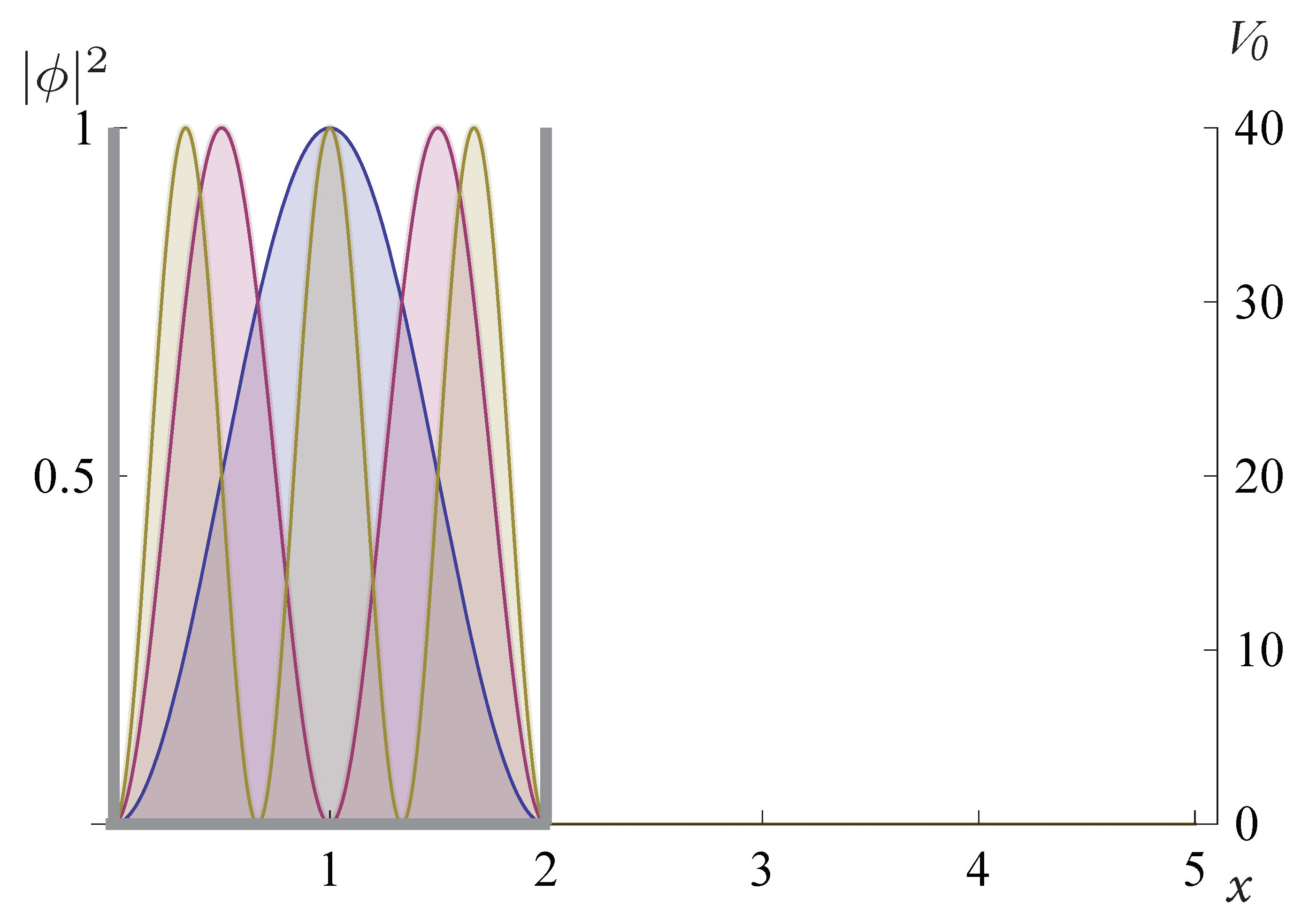
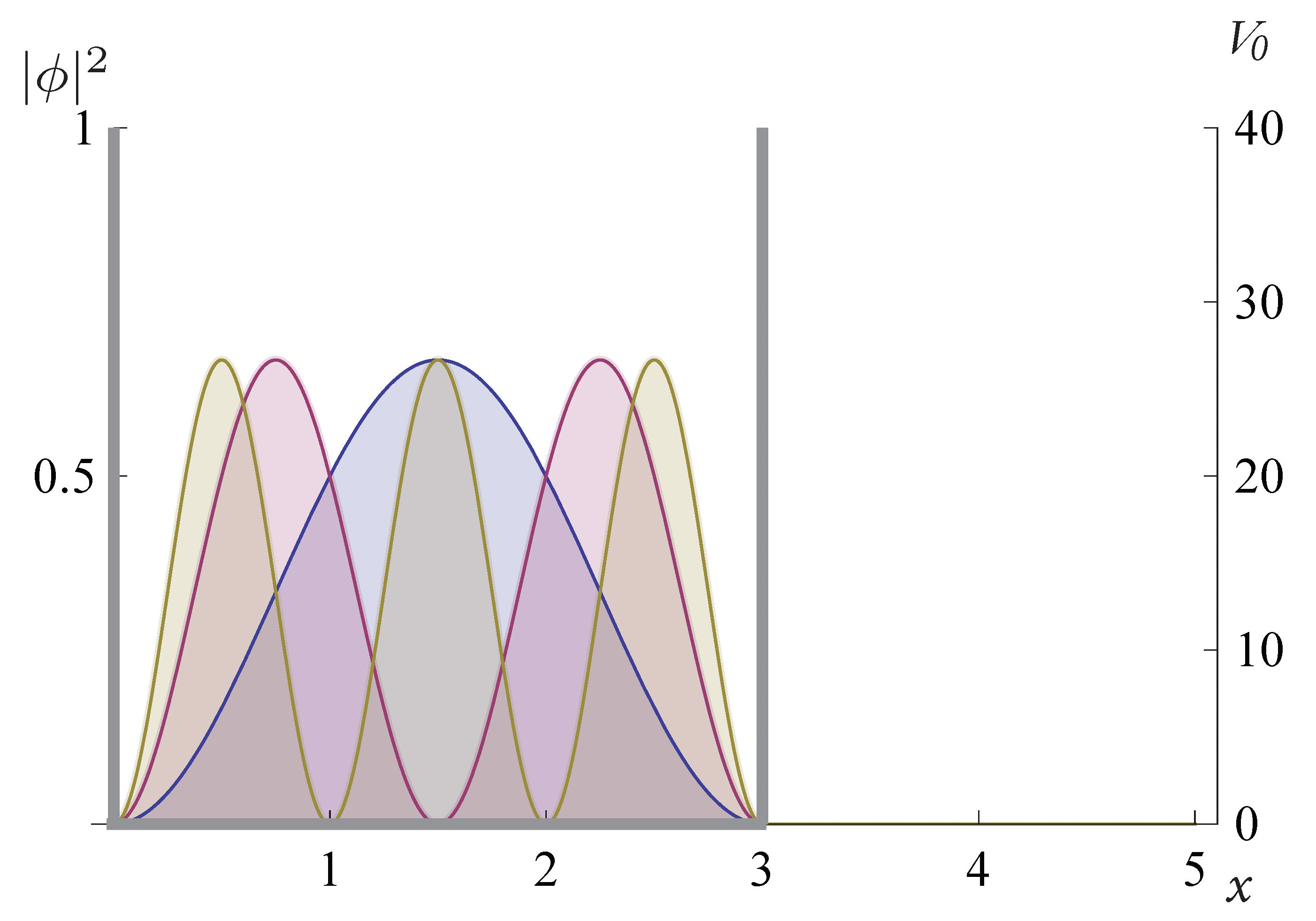
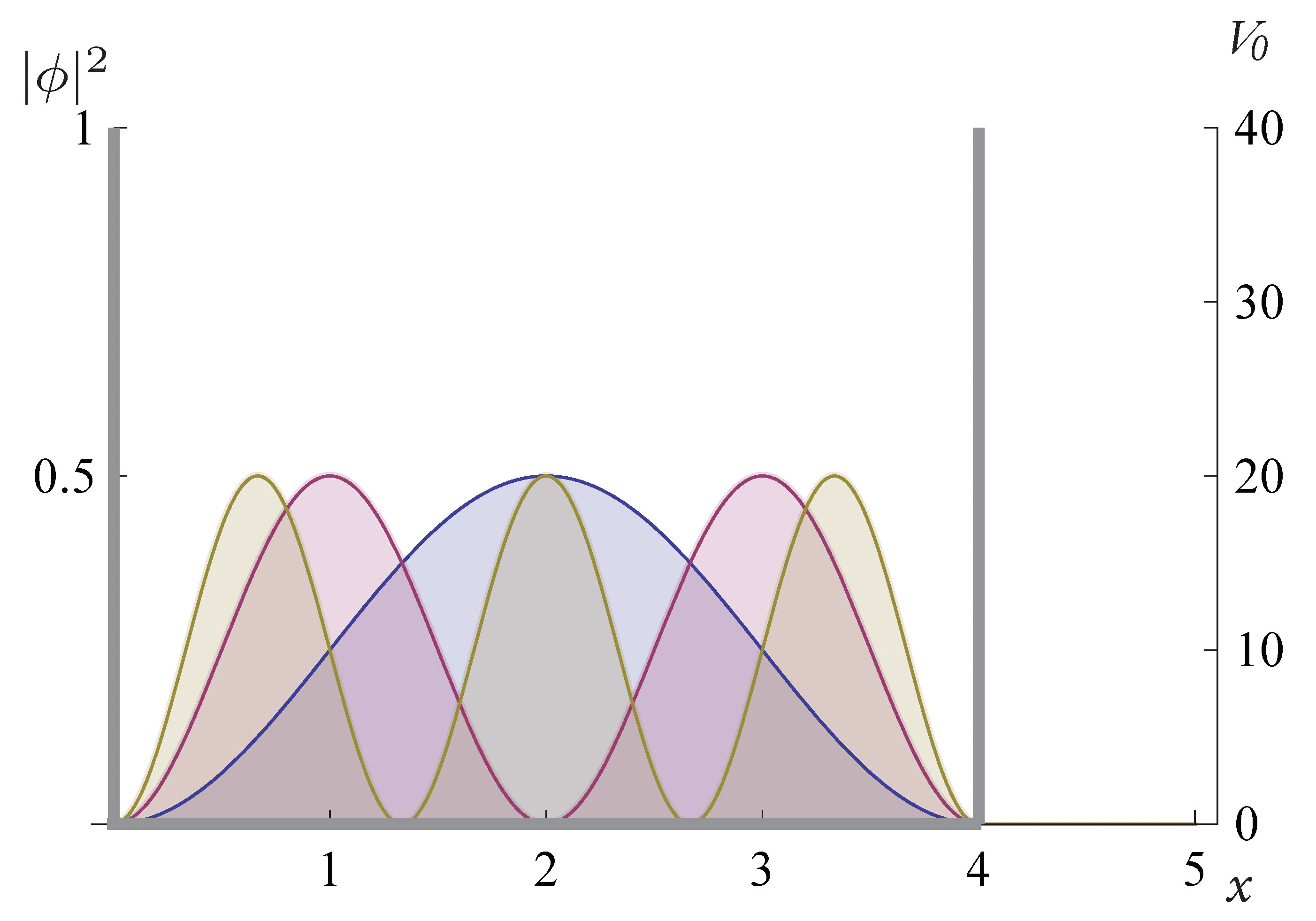
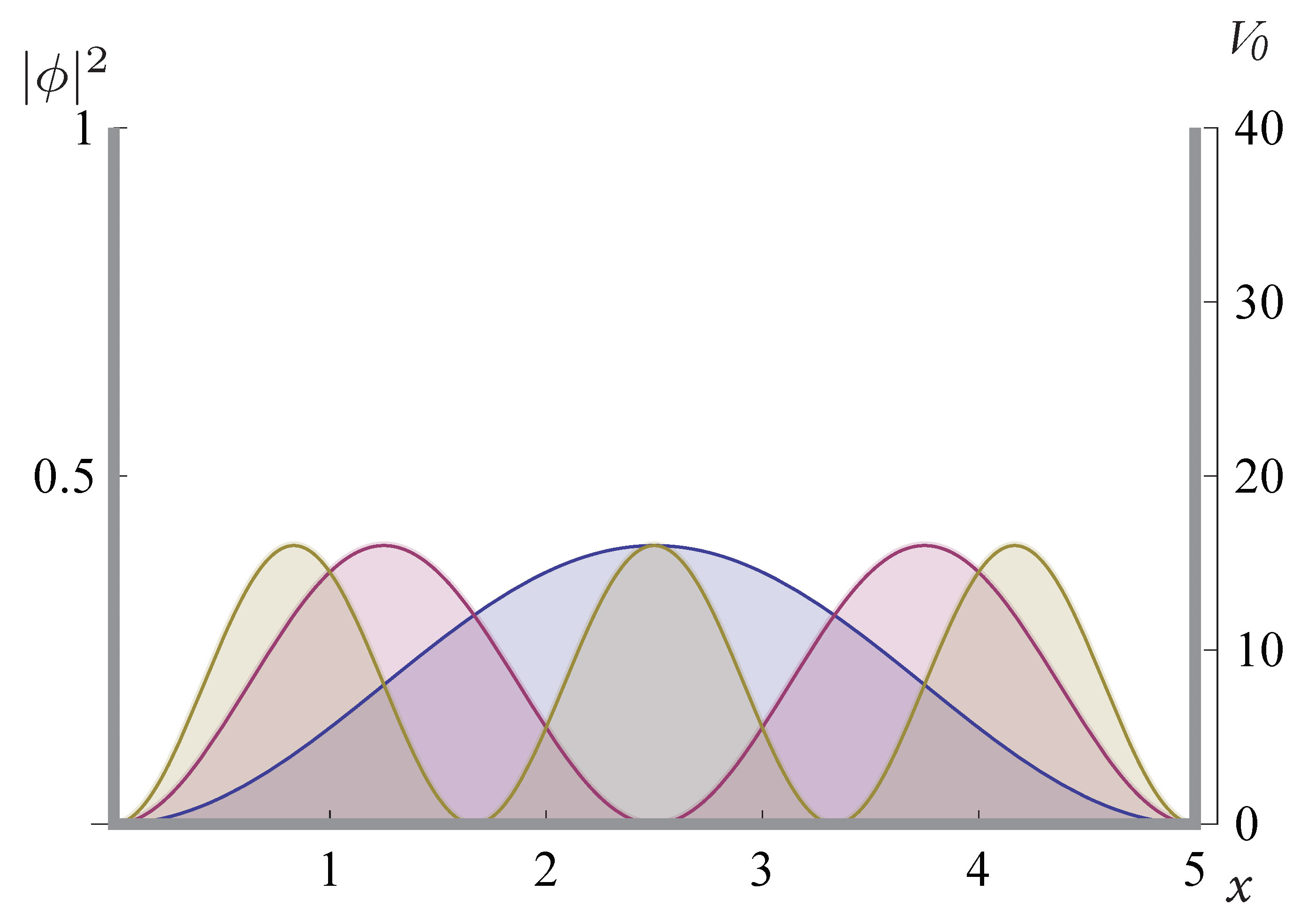
Figure 1: Infinite square-well potential with a moving barrier, see (22). Plot of the probability densities, see (23), $|\phi_{1}|^{2}$ (blue), $|\phi_{2}|^{2}$ (purple), $|\phi_{3}|^{2}$ (yellow), at four different times: $t=1/4$ (top left), $t=1/2$ (top right), $t=3/4$ (bottom left), $t=1$ (bottom right), for the parameter $L=1$.

4 From the infinite well potential with a moving barrier to a Pöschl-Teller potential with a moving barrier

In this section we introduce our second tool, a time dependent SUSY transformation introduced in [8, 9], the notation is adopted from [10]. Then, we apply it to the infinite well potential with a moving barrier to generate a Pöschl-Teller potential with a moving barrier.

4.1 Time dependent supersymmetric quantum mechanics

We start out with a time dependent Schrödinger equation (9) where the potential $V_{0}$ is a real known function. Next, we propose the existence of an operator $\mathcal{L}_{1}$ intertwining two Schrödinger operators

$$S_{1}\mathcal{L}_{1}=\mathcal{L}_{1}S_{0},$$ (24)

where the Schrödinger operators are defined as $S_{j}=i\partial_{t}+\partial_{x}^{2}-V_{j}$, $j=0,1$. Now, if $\mathcal{L}_{1}$ is a differential operator of the form $\mathcal{L}_{1}=A_{1}\left(-\partial_{x}+\frac{u_{x}}{u}\right)$ where $A_{1}=A_{1}(t)$, $u=u(x,t)$ and the subindex in $u_{x}$ represents partial derivation with respect to $x$, then the intertwining relationship (24) and the form of the Schrödinger operators impose the conditions:

$$V_{1}=V_{0}+i(\ln A_{1})_{t}-2(\ln u)_{xx},\qquad i\partial_{t}u+u_{xx}-V_{0}u=c(t),$$ (25)

where $c(t)$ is an integration function. This function $c(t)$ can be absorbed in the potential term, and it will be reflected in the solution $u$ of the Schrödinger equation as a time dependent phase, in this work it will be set $c(t)=0$. Note that now $u$ satisfies $S_{0}u=0$, i.e. it is a solution of the initial system. Furthermore, it can be seen from (25) that in order to avoid new singularities in $V_{1}$, the functions $A_{1}$ and $u$ must not vanish.

The potential $V_{1}$ in (25) is in general a complex function. Since we are interested in a Hermitian operator $S_{1}$, we must ask that the imaginary part of $V_{1}$ vanishes, Im$(V_{1})=0$. Taking (25) and considering $V_{0}$ as a real function, $A_{1}$ and $u$ must also satisfy $i\left(\ln|A_{1}|^{2}\right)_{t}=2\left(\ln(u/u^{*})\right)_{xx}$, since the left hand side depends only on time we can say that

$$\frac{\partial^{3}}{\partial x^{3}}\ln\left(\frac{u}{u^{*}}\right)=0$$ (26)

is a reality condition to generate a Hermitian operator $S_{1}$, and then $|A_{1}|$ is fixed to

$$|A_{1}|=\exp\left\{2\int\text{Im}\left[\frac{\partial^{2}}{\partial x^{2}}\ln u(x,t)\right]dt\right\}.$$ (27)

If this condition is inserted into (25) along with $A_{1}=|A_{1}|$, then the expression of the new potential simplifies to

$$V_{1}=V_{0}-\frac{\partial^{2}}{\partial x^{2}}\ln|u|^{2}.$$ (28)

The intertwining relation (24) ensures that if $\phi$ solves the equation $S_{0}\phi=0$, then $\chi=\mathcal{L}_{1}\phi$ solves $S_{1}\chi=0$. Direct substitution shows that there is an extra function $\chi_{\epsilon}=1/A_{1}u^{*}$, often called missing state, that also solves $S_{1}\chi_{\epsilon}=0$. Consult [8, 9, 10, 11] for more details on this technique.

4.2 Trigonometric Pöschl-Teller potential with a moving barrier

In order to apply a 1-SUSY transformation to the time dependent potential defined in (22), we need to select a transformation function $u(x,t)$ fulfilling three conditions: i) $u(x,t)$ must satisfy the time dependent Schrödinger equation $S_{0}u=0$, ii) $u(x,t)\neq 0$ to avoid new singularities inside the domain of the potential and iii) $\partial_{x}^{3}\ln(u/u^{*})=0$ to generate a Hermitian potential $V_{1}$. One function satisfying all three conditions is $\phi_{1}(x,t)$ in (23), thus, we will use it as transformation function:

$$u(x,t)=\sqrt{\frac{2}{\ell}}\sin\left(\frac{\pi}{\ell}x\right)\exp\left\{i\frac{L}{\ell}\left[x^{2}+\left(\frac{\pi}{2L}\right)^{2}\right]\right\},\qquad\ell=L(4t+1).$$ (29)

Then, we need to calculate the function $A_{1}$, see (27), and the intertwining operator $\mathcal{L}_{1}=A_{1}\left(-\partial_{x}+\frac{u_{x}}{u}\right)$:

$$A_{1}(t)=4t+1,\qquad\mathcal{L}_{1}=-(4t+1)\frac{\partial}{\partial_{x}}+i2x+\frac{\pi}{L}\cot\left(\frac{\pi x}{\ell}\right).$$ (30)

The 1-SUSY partner $V_{1}$ of (22) can be obtained directly from (28) as

$$V_{1}(x,t)=\left\{\begin{array}[]{lll}2\left(\frac{\pi}{\ell}\right)^{2}\csc^{2}\left(\frac{\pi x}{\ell}\right),&&0<x<\ell(t),\\ \infty,&&\text{otherwise},\end{array}\right.$$ (33)

it coincides with a trigonometric Pöschl-Teller potential at any fixed time [21], emphasizing that in our situation the potential has a moving wall. Solutions of the time dependent Schrödinger equation for this potential can be obtain applying the operator $\mathcal{L}_{1}$ onto solutions $\phi_{n}$, see (23) and (30):

$$\chi_{n}(x,t)=\mathcal{L}_{1}\phi_{n}(x,t)$$

$$=\frac{\pi}{L}\sqrt{\frac{2}{\ell}}\left[\cot\left(\frac{\pi x}{\ell}\right)\sin\left(\frac{n\pi x}{\ell}\right)-n\cos\left(\frac{n\pi x}{\ell}\right)\right]\exp\left\{i\frac{L}{\ell}\left[x^{2}+\left(\frac{n\pi}{2L}\right)^{2}\right]\right\},$$ (34)

where $n=2,3,4,\cdots$. In this problem $\lim_{x\to 0}\chi_{n}(x,t)=\lim_{x\to\ell}\chi_{n}(x,t)=0$. There is no square integrable missing state $\chi_{\epsilon}$. In Fig. 2 the Pöschl-Teller potential with a moving barrier and the normalized probability densities corresponding to $\chi_{2}$, $\chi_{3}$ and $\chi_{4}$ are shown at four different times $t=1/4,~{}1/2,~{}3/4,~{}1$, for the parameter $L=1$.

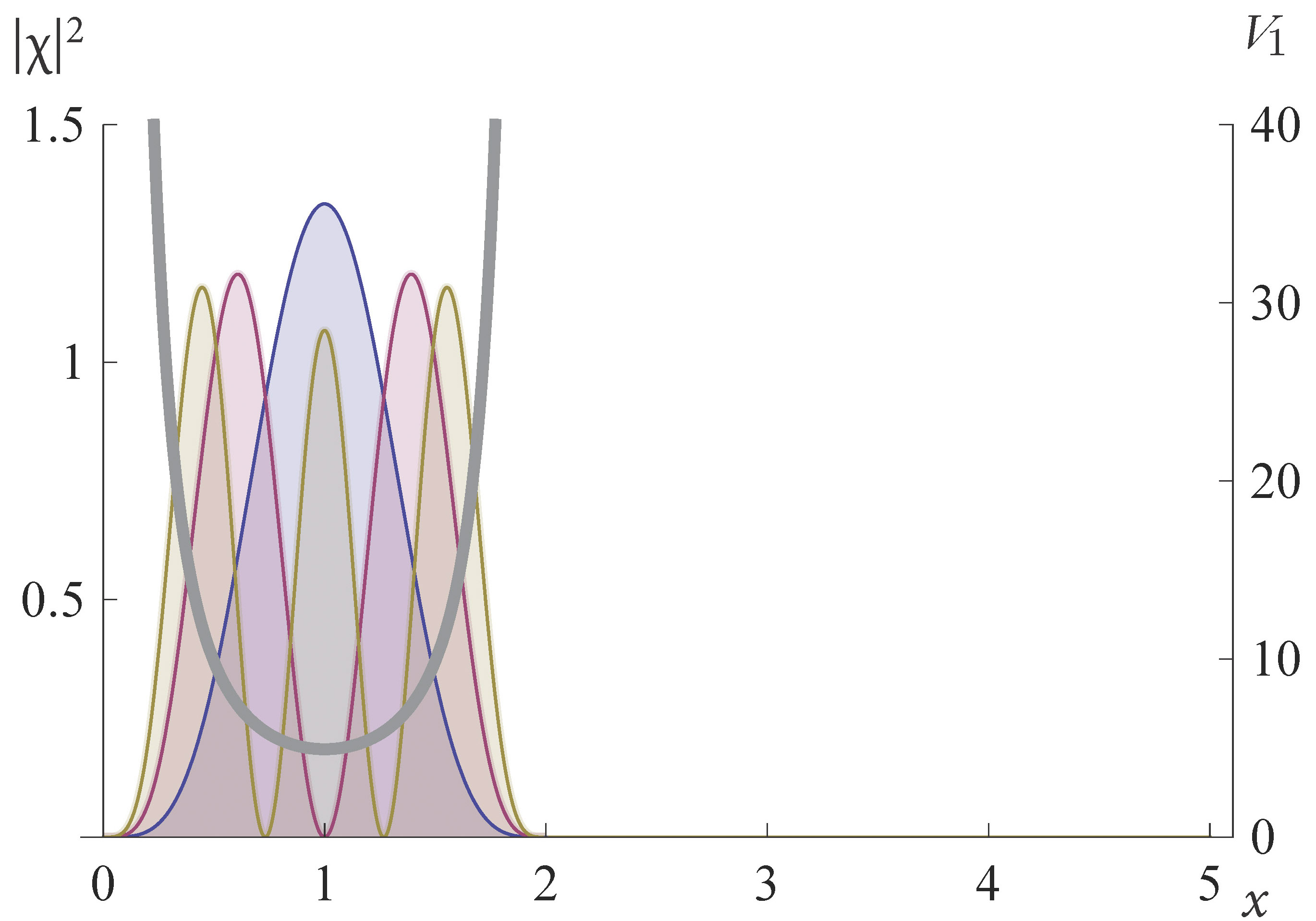
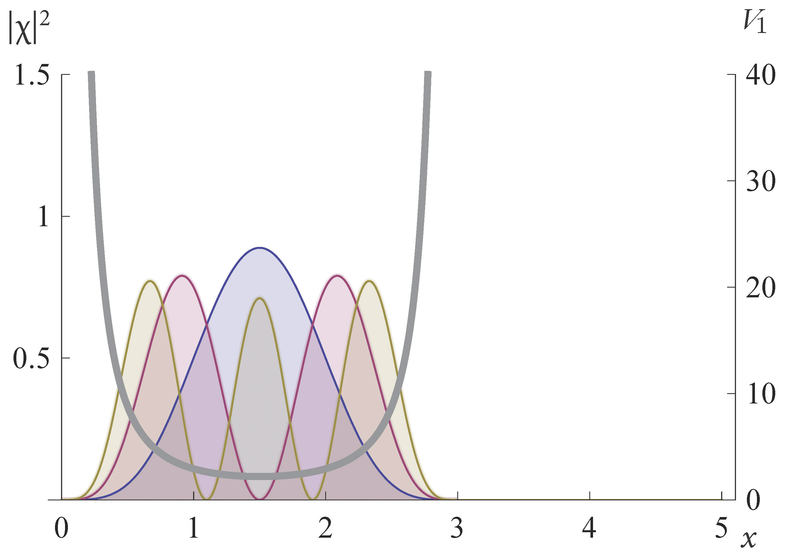
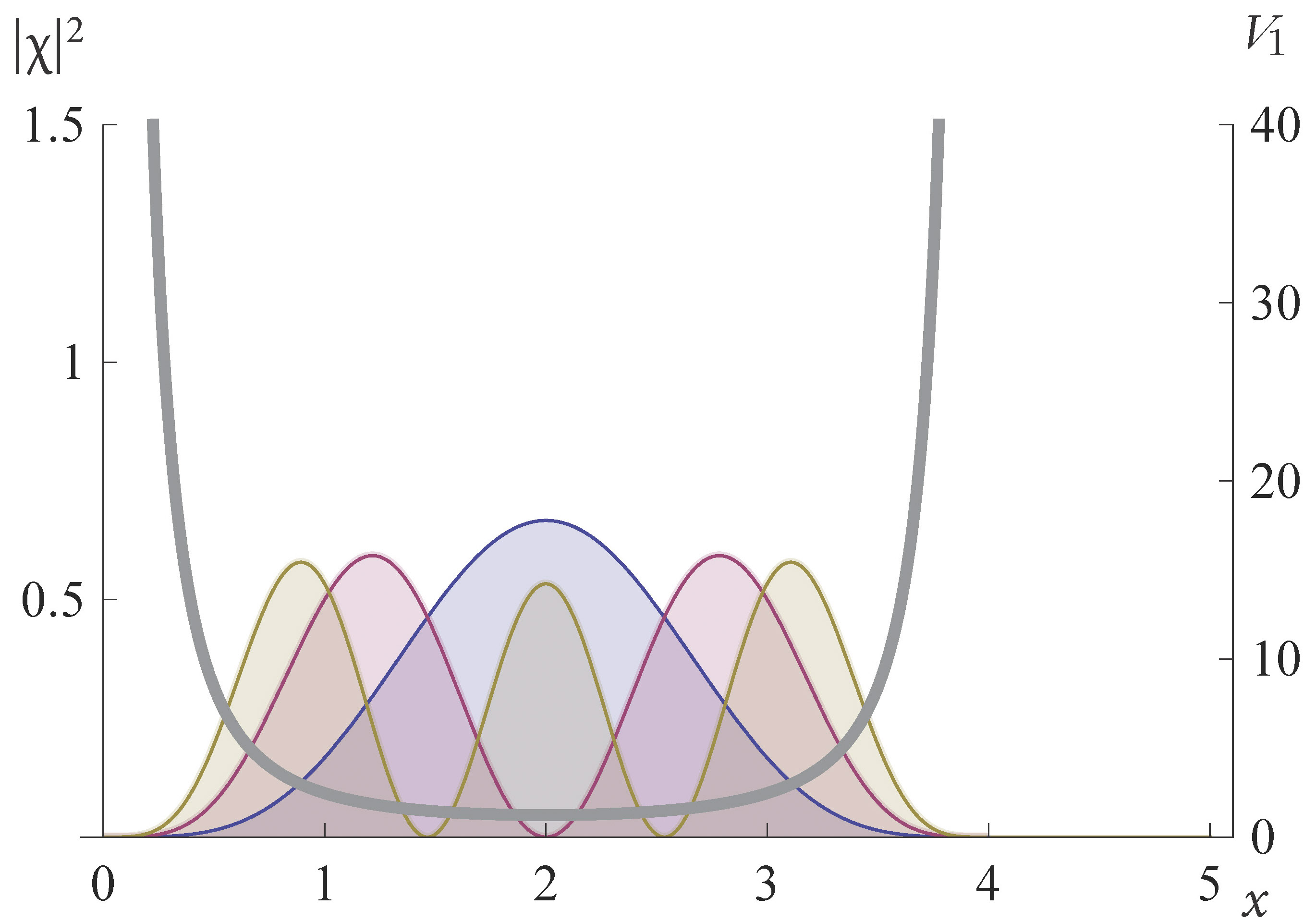
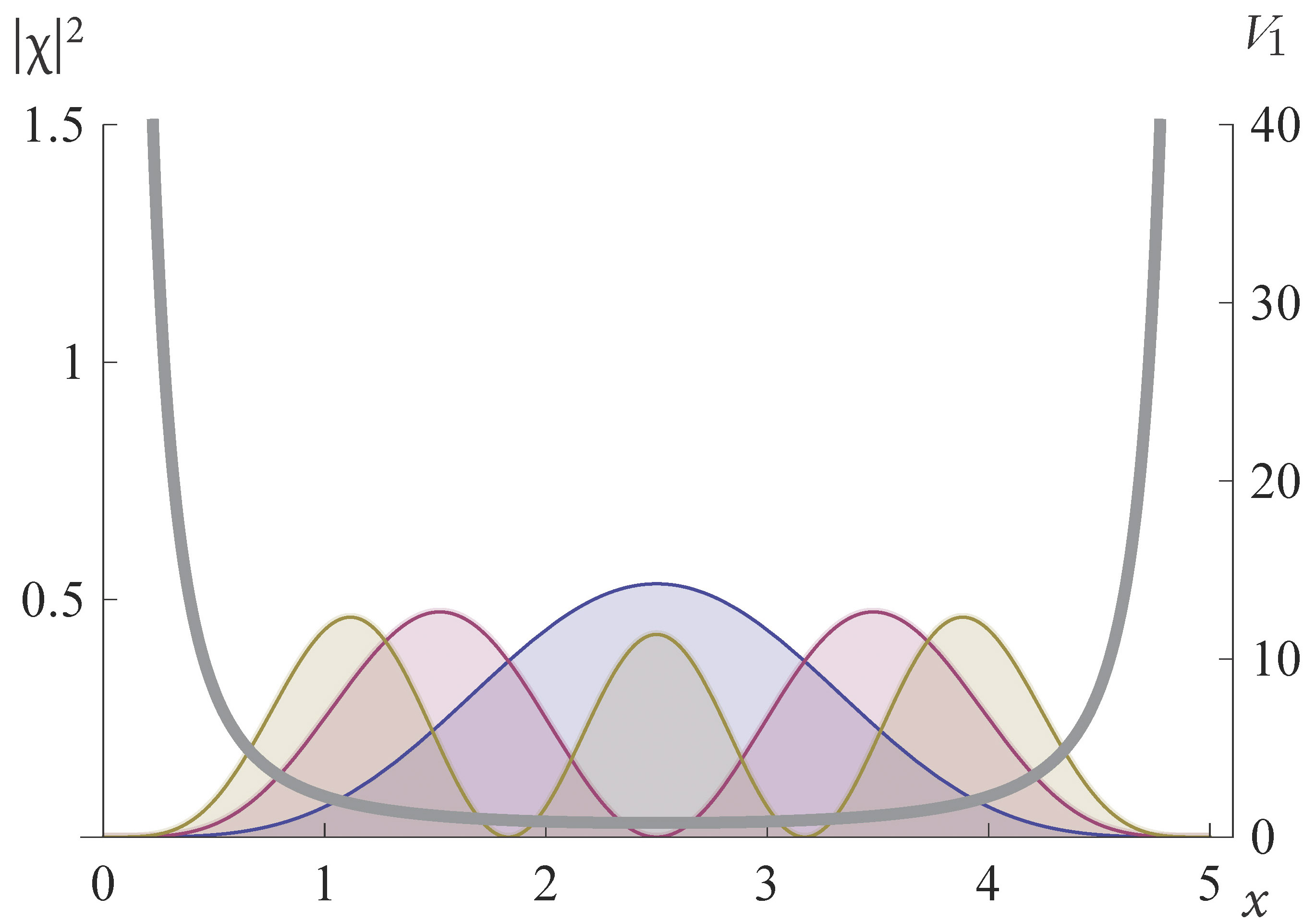
Figure 2: In gray a trigonometric Pöschl-Teller potential with a moving barrier, see (33). Moreover, normalized probability densities are also plotted, see (34), $|\chi_{2}|^{2}$ (blue), $|\chi_{3}|^{2}$ (purple), $|\chi_{4}|^{2}$ (yellow), at four different times: $t=1/4$ (top left), $t=1/2$ (top right), $t=3/4$ (bottom left), $t=1$ (bottom right), for the parameter $L=1$.

5 Confluent SUSY partners: more potentials with a moving barrier

The 1-SUSY technique introduced in Sec. 4 has as constraint that the transformation function $u$ must never vanish. To underpass this restriction a second iteration can be performed, the particular iteration we will use is known as confluent SUSY, see [10] for the time dependent version and [22] for the time independent case. This technique will be applied again to $V_{0}$ and will generate a new family of infinite potential wells with a moving barrier.

5.1 Time dependent confluent SUSY

Departing from $S_{1}$ we propose a second intertwining operator $\mathcal{L}_{2}$ connecting $S_{1}$ with a new Schrödinger operator $S_{2}$

$$S_{2}\mathcal{L}_{2}=\mathcal{L}_{2}S_{1},$$ (35)

where again $\mathcal{L}_{2}$ is a differential operator on the form $\mathcal{L}_{2}=A_{2}\left(-\partial_{x}+\frac{v_{x}}{v}\right)$, where $v$ solves $S_{1}v=0$. We would like to use a function $v$ written in term of $u$. If the missing state $\chi_{\epsilon}=1/A_{1}u^{*}$ is used, then the generated potential $V_{2}$ is exactly the initial potential $V_{0}$. In order to generate a different potential we should use a more general solution $v$:

$$v=\frac{1}{A_{1}u^{*}}\left(\omega+\int^{x}_{x_{0}}|u(s,t)|^{2}ds\right),$$ (36)

where $\omega$ is a real constant. It can be verified by direct substitution that this general expression for $v$ is indeed a solution of $S_{1}v=0$. We can also demand $S_{2}$ and $S_{1}$ to be Hermitian operators. This directly implies $\partial^{3}_{x}\ln(v/v^{*})=0$, and substituting (36), the Hermiticity condition for the second potential is also $\partial^{3}_{x}\ln(u/u^{*})=0$. Analogous to (27), since $\omega$ was chosen real, $A_{2}$ can be fixed as $A_{2}=A_{1}$. Under these considerations the new potential is given by

$$V_{2}=V_{1}-2\partial_{xx}\ln|v|=V_{0}-2\partial_{xx}\ln\left(\omega+\int^{x}_{x_{0}}|u(s,t)|^{2}ds\right).$$ (37)

From the intertwining relation (35) and using the functions $\chi_{n}$ (solving $S_{1}\chi=0$), we can see that functions $\xi_{n}=\mathcal{L}_{2}\chi_{n}=\mathcal{L}_{2}\mathcal{L}_{1}\phi_{n}$ will solve the equation $S_{2}\xi=0$. Finally, a missing solution can be found as

$$\xi_{\epsilon}=\frac{1}{A_{2}v^{*}}=\frac{u}{\omega+\int^{x}_{x_{0}}|u(s,t)|^{2}ds}.$$ (38)

Confluent and 1-SUSY techniques present similarities. Indeed, both use only one transformation function $u$ fulfilling $S_{0}u=0$, both require $\partial_{x}^{3}\ln(u/u^{*})=0$ to generate Hermitian potentials, but the regularity condition is different. In 1-SUSY $u$ must be nodeless, for confluent SUSY the transformation function satisfies a more relaxed condition: $\int^{x}_{x_{0}}|u(s,t)|^{2}ds\neq-\omega$, this last condition could be met, for example, by any square integrable solution.

5.2 More potentials with a moving barrier

Departing from the infinite well potential with a moving barrier in (22), we can notice that solutions $\phi_{n}(x,t)$ (see (23)), when $n\geq 2$ cannot be used as transformation function for a 1-SUSY transformation because they have at least one zero in the interval $(0,\ell)$. With the confluent SUSY algorithm presented in this section we can surpass this restriction.

By selecting $u(x,t)=\phi_{m}(x,t)$ (see (23)), where $m\in\mathbb{N}$ is a fixed number, a confluent SUSY partner of the infinite square-well potential with a moving barrier can be constructed. First we need to find the function $A_{2}=A_{1}=|A_{1}|$, see (27), and the intertwining operators $\mathcal{L}_{1}=A_{1}\left(-\partial_{x}+u_{x}/u\right)$ and $\mathcal{L}_{2}=A_{1}\left(-\partial_{x}+v_{x}/v\right)$:

$$A_{2}(t)=A_{1}(t)=4t+1,$$

$$\mathcal{L}_{1}=-(4t+1)\frac{\partial}{\partial_{x}}+i2x+\frac{m\pi}{L}\cot\left(\frac{m\pi x}{\ell}\right),$$

$$\mathcal{L}_{2}=-(4t+1)\frac{\partial}{\partial_{x}}+i2x-\frac{m\pi}{L}\cot\left(\frac{m\pi x}{\ell}\right)+\frac{4m\pi\ell\sin^{2}\left(\frac{m\pi x}{\ell}\right)}{2m\pi L(x+\ell\omega)-L\ell\sin\left(\frac{2m\pi x}{\ell}\right)},$$ (39)

where we fixed $x_{0}=0$ in the definition of $v$, see (36), (37) and (38). Then, using (37) an expression for the potential $V_{2}$ can be obtained:

$$V_{2}(x,t)=\left\{\begin{array}[]{lll}\frac{32\left(\frac{m\pi}{\ell}\right)^{2}\sin\left(\frac{m\pi x}{\ell}\right)\left[\sin\left(\frac{m\pi x}{\ell}\right)-\frac{m\pi}{\ell}\cos\left(\frac{m\pi x}{\ell}\right)(x+\omega\ell)\right]}{\left[\sin\left(\frac{2m\pi x}{\ell}\right)-2\frac{m\pi}{\ell}(x+\omega\ell)\right]^{2}},&&0<x<\ell(t),\\ \infty,&&\text{otherwise},\end{array}\right.$$ (42)

where $\omega\in(\infty,-1]\cup[0,\infty)$ is a constant introduced by confluent algorithm.

Solutions $\xi_{n}(x,t)$ for these potentials can as well be found with help of intertwining operators $\mathcal{L}_{1}$ and $\mathcal{L}_{2}$, see (23) and (39)), when $n\neq m$:

$$\xi_{n}(x,t)=\mathcal{L}_{2}\mathcal{L}_{1}\phi_{n}$$

$$=\left(\frac{\pi}{L}\right)^{2}\sqrt{\frac{2}{\ell}}\sin\left(\frac{n\pi}{\ell}x\right)\exp\left\{i\frac{L}{\ell}\left[x^{2}+\left(\frac{n\pi}{2L}\right)^{2}\right]\right\}$$

$$\times\vspace{-1cm}\frac{\left[(m^{2}+n^{2})\sin\left(\frac{2m\pi x}{\ell}\right)+\frac{2m\pi}{\ell}(m^{2}-n^{2})(x+\omega\ell)\right]-4mn\ell\cot\left(\frac{n\pi x}{\ell}\right)\sin^{2}\left(\frac{m\pi x}{\ell}\right)}{\frac{2m\pi}{\ell}(x+\omega\ell)-\sin\left(\frac{2m\pi x}{\ell}\right)}.$$ (43)

If $n=m$, then the corresponding solution is the missing state $\xi_{\epsilon}(x,t)$ (see (38)):

$$\xi_{\epsilon}(x,t) = \sqrt{\frac{2}{\ell}}\sin\left(\frac{m\pi}{\ell}x\right)$$ (44)

$$\times\exp\left\{i\frac{L}{\ell}\left[x^{2}+\left(\frac{m\pi}{2L}\right)^{2}\right]\right\}\frac{2m\pi}{\frac{2m\pi}{\ell}(x+\ell\omega)-\sin\left(\frac{2m\pi x}{\ell}\right)}.$$

Solutions $\xi_{n}$ satisfy $\lim_{x\to 0}\xi_{n}(x,t)=\lim_{x\to\ell}\xi_{n}(x,t)=0$ whereas $\xi_{\epsilon}$ fulfills $\lim_{x\to 0}\xi_{\epsilon}(x,t)=\lim_{x\to\ell}\xi_{\epsilon}(x,t)=0$ only if $\omega\neq-1,0$. When $\omega$ is set equal to $-1$ or zero, the function $\xi_{\epsilon}$ is not square integrable. The confluent SUSY partner of the infinite square-well potential with fixed barriers $\widetilde{V}(y)$, see (4), are reported in [23, 24], the potentials $V_{2}(x,t)$ are a dynamic version of them. In Fig. 3 the potential $V_{2}$ in (42) is illustrated, the parameters used where $L=1$, $\omega=0.4$ and $m=2$. This system has sharp edges at $x=0$ and $x=\ell$. Normalized probability densities of three solutions are shown as well, corresponding to $\xi_{1}$, $\xi_{\epsilon}$ and $\xi_{3}$. For the special cases $\omega=-1$ and $\omega=0$ one of the edges of $V_{2}$ is smooth while the other is sharp, as can be seen in Fig. 4 and Fig. 5, moreover these special situations does not present a square integrable missing state $\xi_{\epsilon}$.

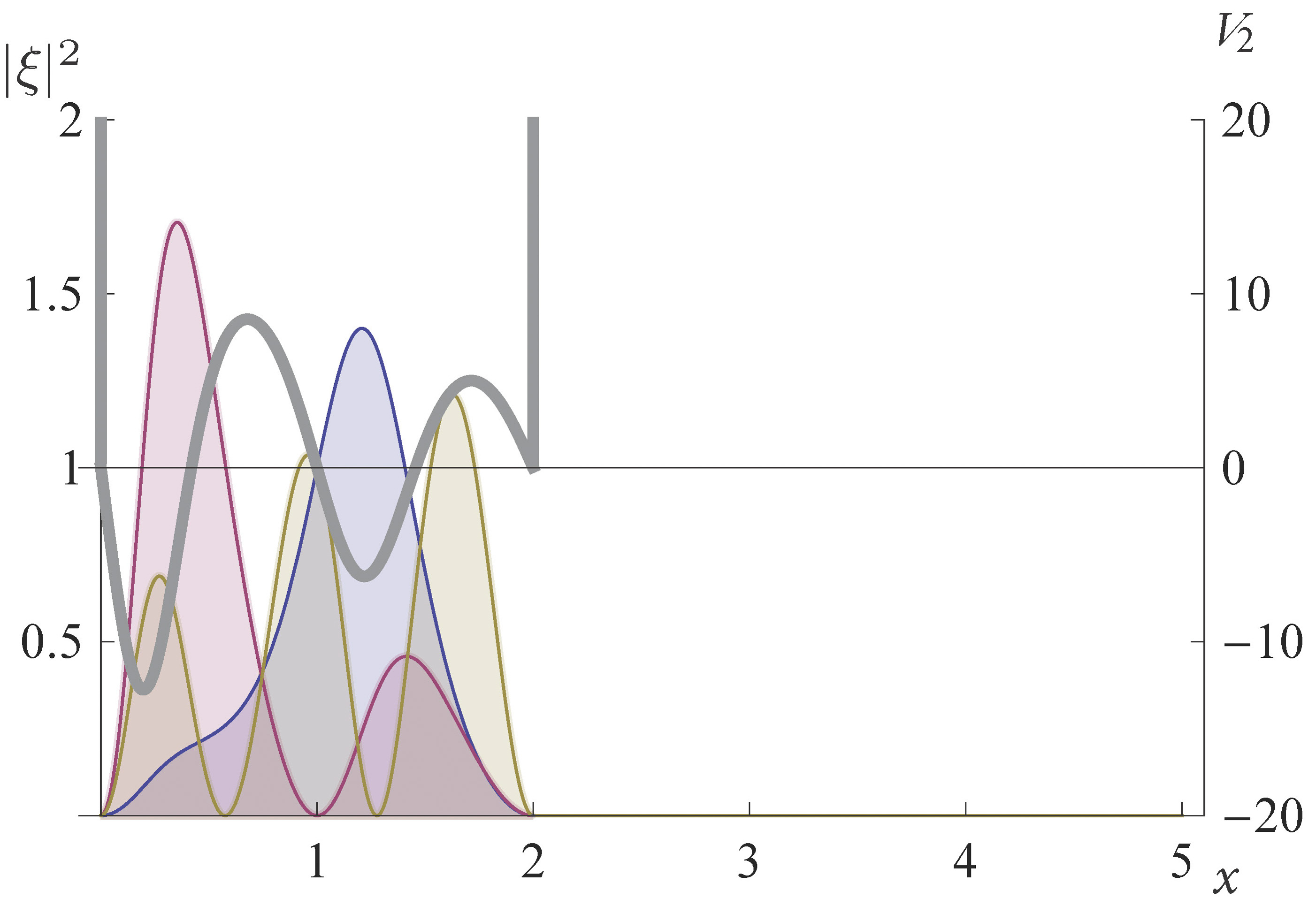
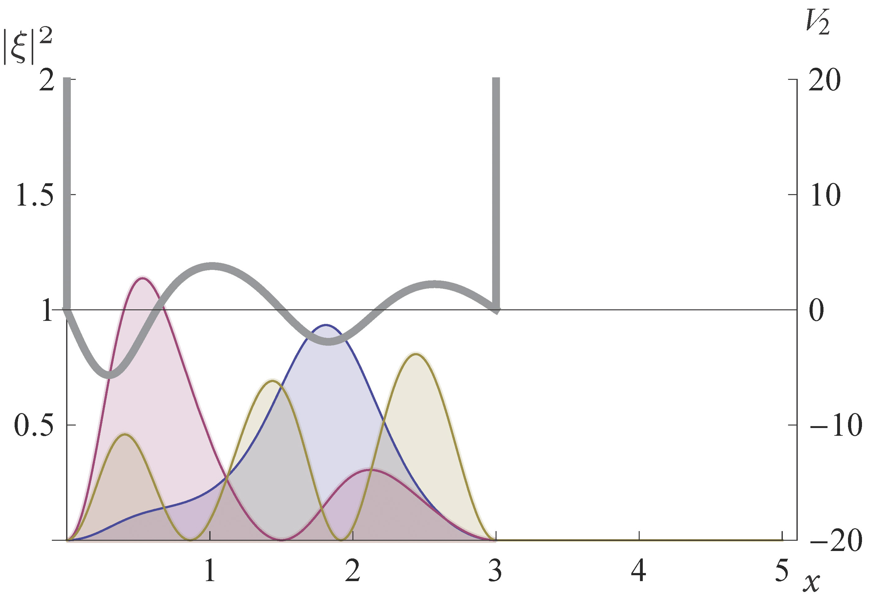
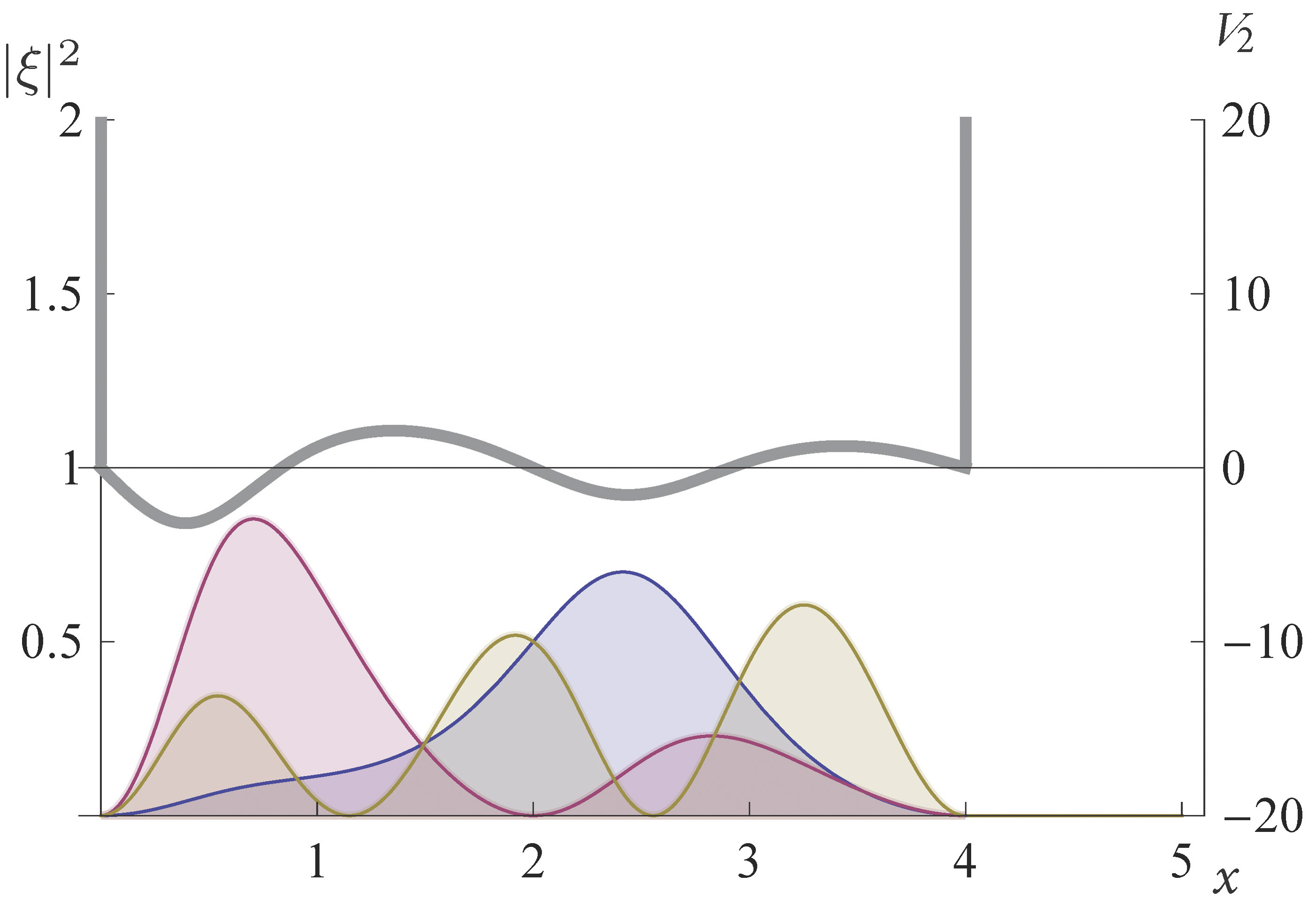
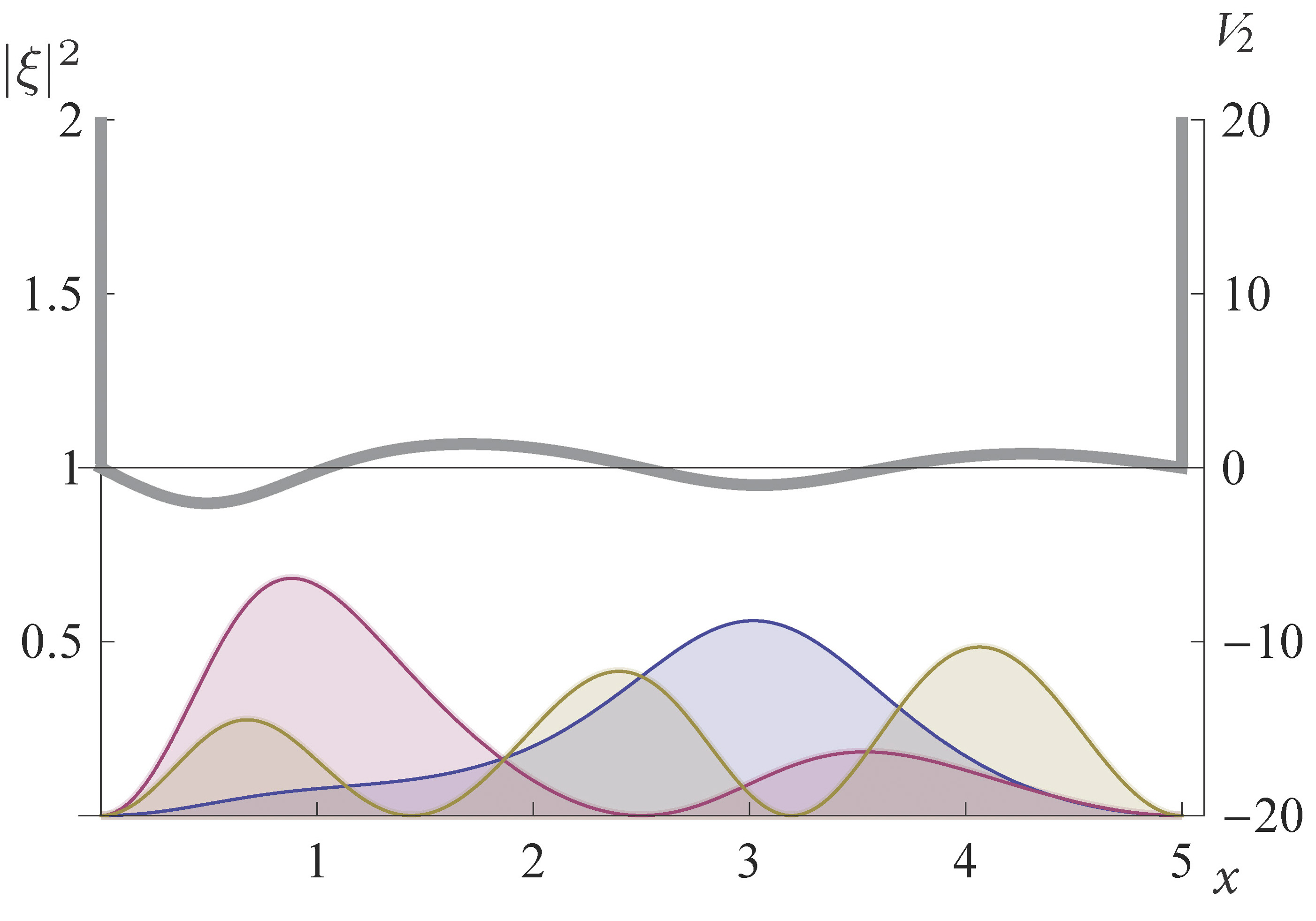
Figure 3: In gray a confluent SUSY partner of the infinite square-well potential with a moving barrier, see (42). Moreover, normalized probability densities are also plotted, see (43) and (44), $|\xi_{1}|^{2}$ (blue), $|\xi_{\epsilon}|^{2}$ (purple), $|\xi_{3}|^{2}$ (yellow), at four different times: $t=1/4$ (top left), $t=1/2$ (top right), $t=3/4$ (bottom left), $t=1$ (bottom right), for the parameters $L=1$, $\omega=0.4$ and $m=2$.

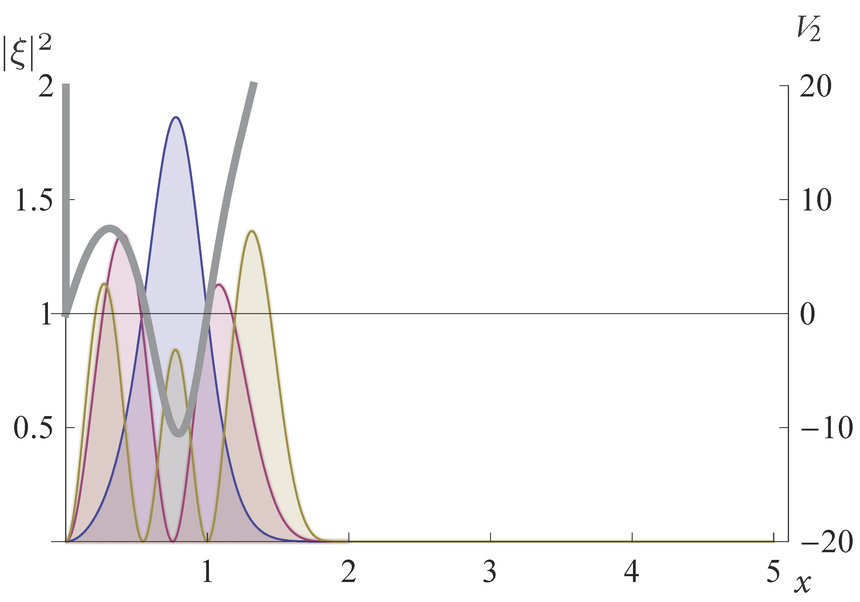
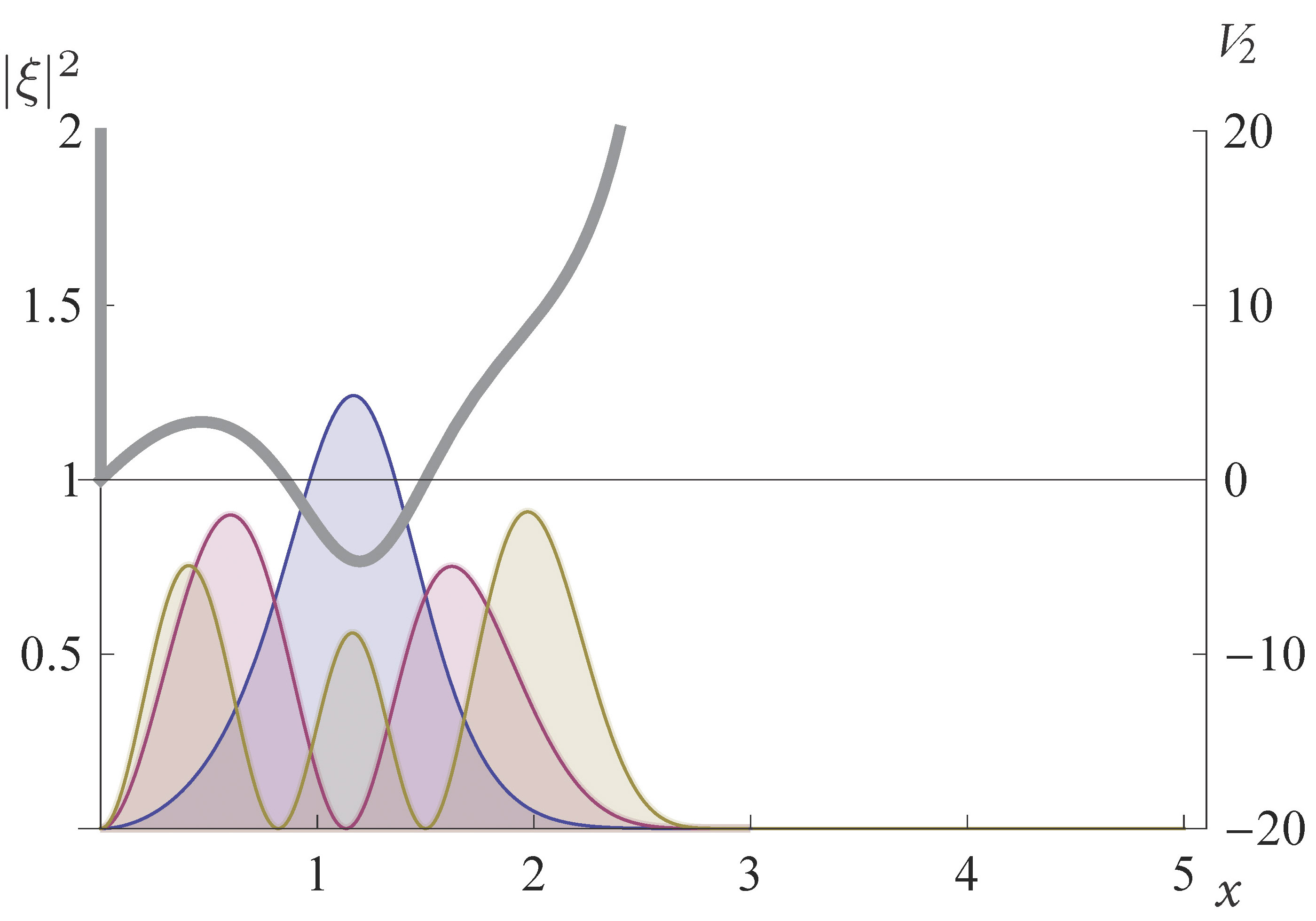
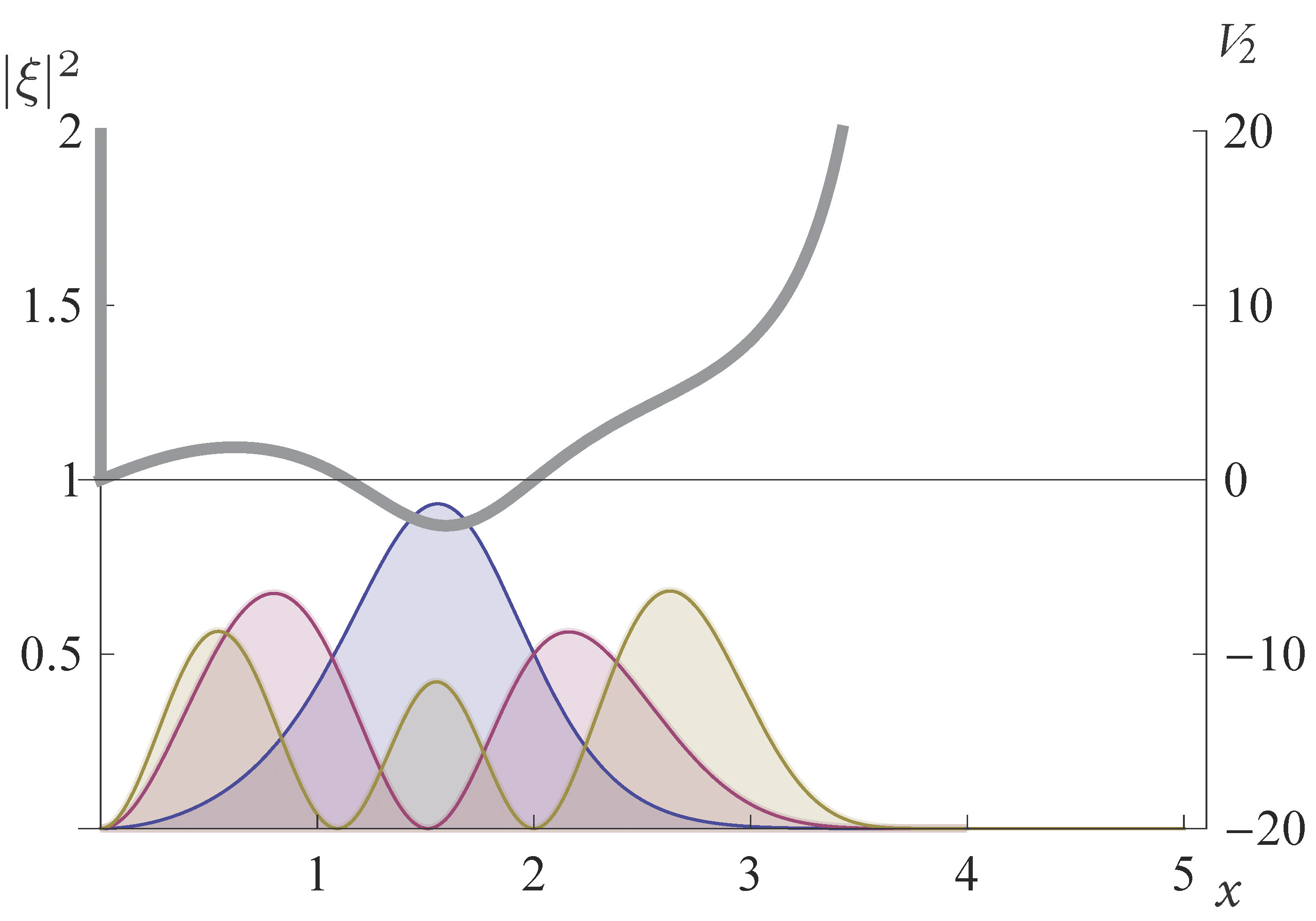
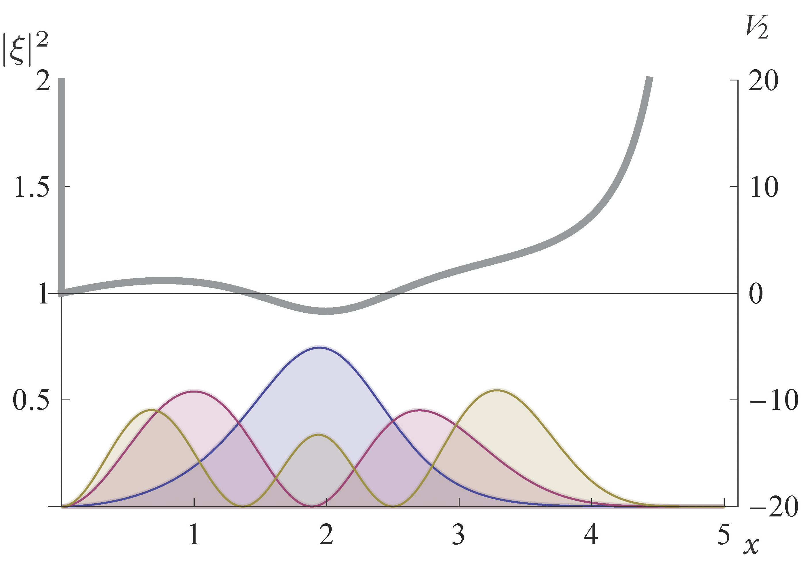
Figure 4: In gray a confluent SUSY partner of the infinite square-well potential with a moving barrier, see (42). Moreover, normalized probability densities are also plotted, see (43), $|\xi_{1}|^{2}$ (blue), $|\xi_{3}|^{2}$ (purple), $|\xi_{4}|^{2}$ (yellow), at four different times: $t=1/4$ (top left), $t=1/2$ (top right), $t=3/4$ (bottom left), $t=1$ (bottom right), for the parameters $L=1$, $\omega=-1$ and $m=2$.

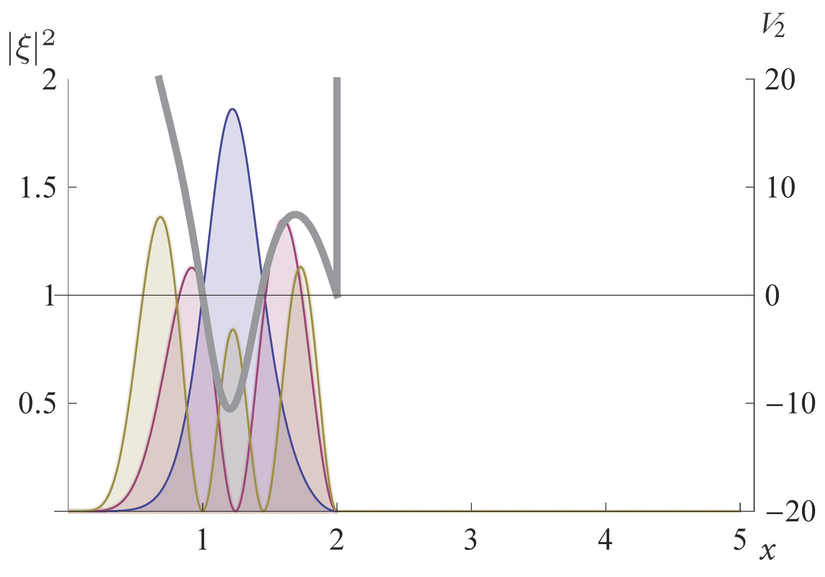
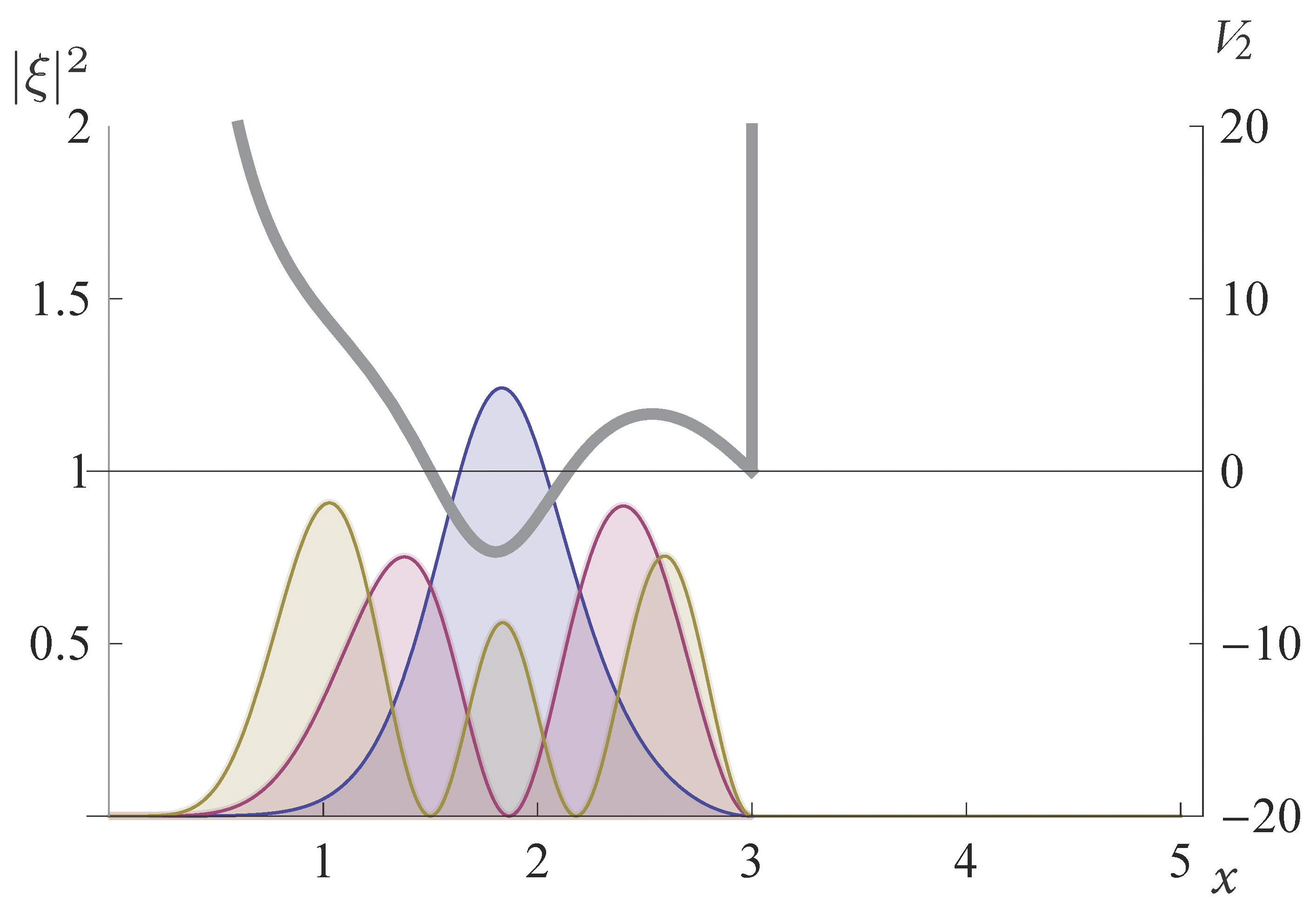
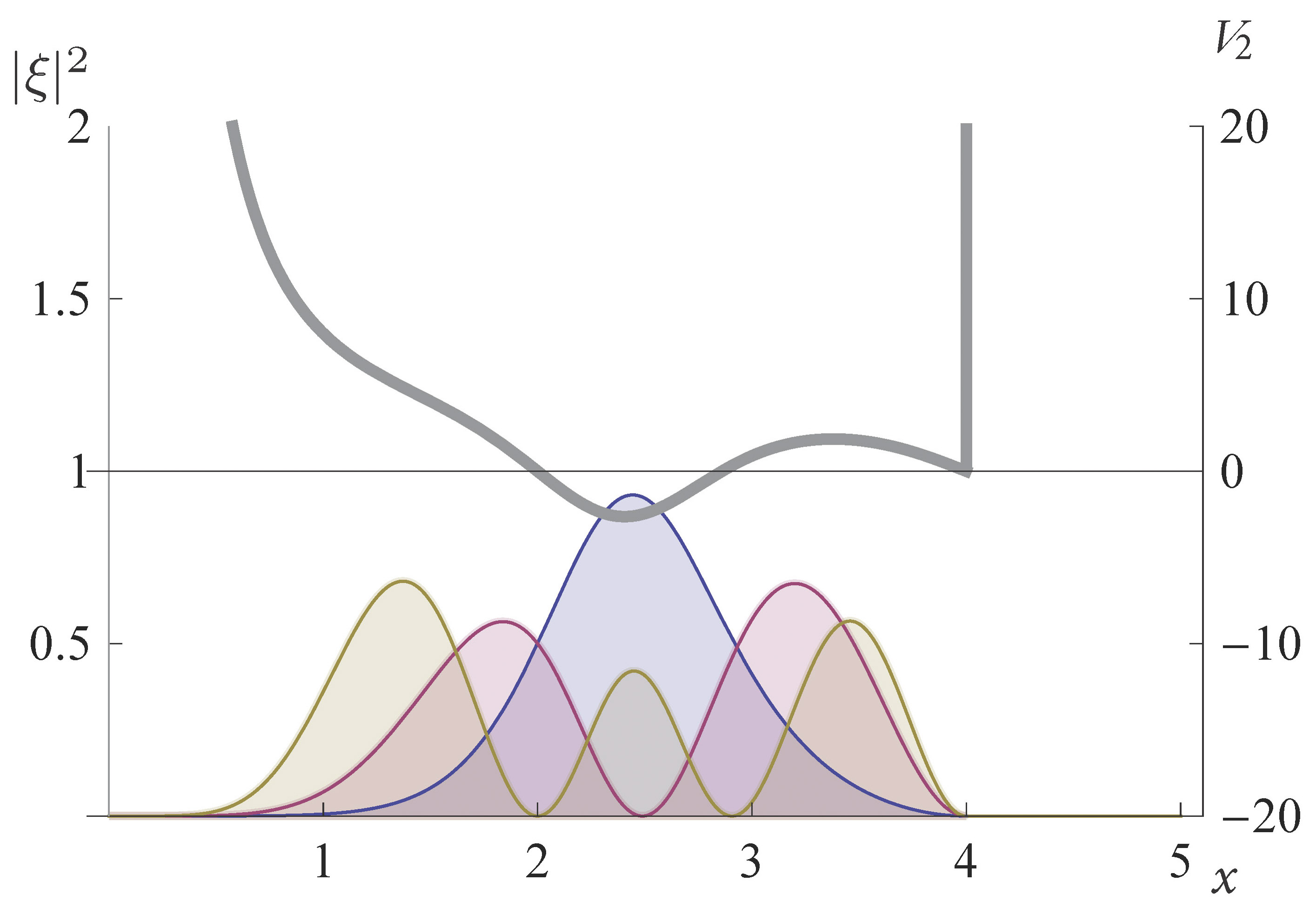
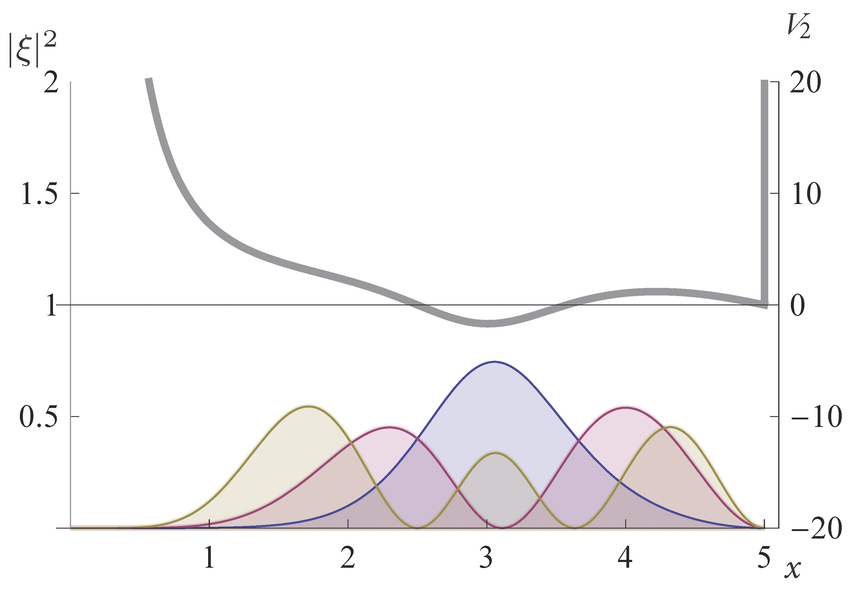
Figure 5: In gray a confluent SUSY partner of the infinite square-well potential with a moving barrier, see (42). Moreover, normalized probability densities are also plotted, see (43), $|\xi_{1}|^{2}$ (blue), $|\xi_{3}|^{2}$ (purple), $|\xi_{4}|^{2}$ (yellow), at four different times: $t=1/4$ (top left), $t=1/2$ (top right), $t=3/4$ (bottom left), $t=1$ (bottom right), for the parameters $L=1$, $\omega=0$ and $m=2$.

6 Conclusions

In this article we showed how to generate different infinite potential wells with a moving boundary condition. Through a series of transformations, we obtained the infinite square-well potential, a trigonometric Pöschl-Teller potential and the confluent SUSY partners of the infinite square-well potential, where one of the barriers is fixed and the other is moving with a constant velocity. For all these systems, exact solutions of the time dependent Schrödinger equations fulfilling the moving boundary conditions were given in a closed form.

As a continuation of the present work, it would be interesting to study different sets of coherent and squeezed states for the constructed systems and the calculation of relevant physical quantities and mathematical properties of such states.

References

- [1] J. Crank, Free and moving boundary problems. Clarendon Press, Oxford (1984)
- [2] E. Fermi, On the origin of the cosmic radiation, Phys. Rev., 75, 1169–1174 (1949)
- [3] S. M. Ulam, On some statistical properties of dynamical systems, Proc. Fourth Berkeley Symp. on Math. Statist. and Prob. (Univ. of Calif. Press), 3 , 315–320 (1961)
- [4] J. R. Ray, Exact solutions to the time-dependent Schrödinger equation, Phys. Rev. A, 26, 729–733 (1982)
- [5] G. W. Bluman, On mapping linear partial differential equations to constant coefficient equations, SIAM Journal on Applied Mathematics, 43, 1259–1273 (1983)
- [6] F. Cooper, A. Khare, U. Sukhatme, Supersymmetry and quantum mechanics, Physics Reports, 251, 267–385 (1995)
- [7] D. J. Fernández C., Supersymmetric quantum mechanics, AIP Conf. Proc., 1287, 3–36 (2010)
- [8] V. B. Matveev, M. A. Salle, Darboux transformations and solitons. Springer-Verlag, Berlin (1991)
- [9] V. G. Bagrov, B. F. Samsonov, L. A. Shekoyan, Darboux transformation for the nonsteady Schrödinger equation, Russ. Phys. J., 38, 706–712 (1995)
- [10] A. Contreras-Astorga, A time-dependent anharmonic oscillator, IOP Conf. Series: Journal of Physics: Conf. Series, 839, 012019 (2017)
- [11] K. Zelaya, O. Rosas-Ortiz, Exactly solvable time-dependent oscillator-like Potentials Generated by Darboux transformations, IOP Conf. Series: Journal of Physics: Conf. Series, 839, 012018 (2017)
- [12] F. Finkel, A. González-López, N. Kamran, M. A. Rodríguez, On form-preserving transformations for the time-dependent Schrödinger equation, Journal of Mathematical Physics, 40, 3268–3274 (1999)
- [13] C. Cohen-Tannoudji, B. Diu, F. Laloe, Quantum mechanics Vol. I. Wiley & Sons and Hermann, Paris (1977)
- [14] R. Shankar, Principles of quantum mechanics. Plenum Press, New York (1994)
- [15] L. D. Landau, E. M. Lifshitz, Quantum mechanics non-relativistic theory. Pergamon Press, Exeter (1991)
- [16] A. Schulze-Halberg, B. Roy, Time dependent potentials associated with exceptional orthogonal polynomials, J. Math. Phys., 55, 123506 (2014)
- [17] S. W. Doescher, M. H. Rice, Infinite square-well potential with a moving wall, Am. J. Phys., 37, 1246–1249 (1969)
- [18] D. N. Pinder, The contracting square quantum well, Am. J. Phys., 58, 54–58 (1990)
- [19] M. L. Glasser, J. Mateo, J. Negro, L. M. Nieto, Quantum infinite square well with an oscillating wall, Chaos, Solitons and Fractals, 41, 2067–2074 (2009)
- [20] O. Fojón, M. Gadella, L. P. Lara, The quantum square well with moving boundaries: A numerical analysis, Comput. Math. Appl., 59, 964–976 (2010)
- [21] A. Contreras-Astorga, D. J. Fernández C., Supersymmetric partners of the trigonometric Pöschl–Teller potentials, J. Phys. A: Math. Theor., 41, 475303 (2008)
- [22] D. J. Fernández C., E. Salinas-Hernández,The confluent algorithm in second-order supersymmetric quantum mechanics, J. Phys. A: Math. Theor., 36, 2537–2543 (2003)
- [23] D. J. Fernández, V. Hussin, O. Rosas-Ortiz, Coherent states for Hamiltonians generated by supersymmetry, J. Phys. A: Math. Theor., 40, 6491 (2007)
- [24] M-A Fiset, V. Hussin., Supersymmetric infinite wells and coherent states, J. Phys.: Conf. Ser., 624, 012016 (2015)