Spectroscopy of Extremal (and Near-Extremal) Kerr Black Holes

Abstract

We investigate linear, spin-field perturbations of Kerr black holes in the extremal limit throughout the complex-frequency domain. We calculate quasi-normal modes of extremal Kerr, as well as of near-extremal Kerr, via a novel approach: using the method of Mano, Suzuki and Takasugi (MST). We also show how, in the extremal limit, a branch cut is formed at the superradiant-bound frequency, $\omega_{\text{SR}}$, via a simultaneous accumulation of quasi-normal modes and totally-reflected modes. For real frequencies, we calculate the superradiant amplification factor, which yields the amount of rotational energy that can be extracted from a black hole. In the extremal limit, this factor is the largest and it displays a discontinuity at $\omega_{\text{SR}}$ for some modes. Finally, we find no exponentially-growing modes nor branch points on the upper-frequency plane in extremal Kerr after a numerical investigation, thus providing evidence of the mode-stability of this space-time away from the horizon.

I Introduction

Extremal (i.e., maximally-rotating) Kerr black holes play a special role within theories of gravity. From a theoretical point of view, the Bekenstein-Hawking entropy for extremal black holes can be reproduced via a counting of microstates within String Theory Strominger and Vafa (1996). Furthermore, extremal black holes exhibit a near-horizon enhanced symmetry Bardeen and Horowitz (1999), which has led to the Kerr/Conformal Field Theory correspondence conjecture Guica et al. (2009). Extremal black holes also enjoy a special place in relation to the (weak) Cosmic Censorship conjecture Penrose (1969), in the sense that they are the “last frontier” between rotating black holes and naked singularities. From an observational point of view, there is evidence of astrophysical black holes which are highly spinning Gou et al. (2014); McClintock et al. (2006); Reynolds (2013), for which exact extremality cannot be excluded. Interestingly, high spins lead to a distinct observational feature in the gravitational waveform when a particle is in a near-horizon inspiral into a near-extremal Kerr (NEK) black hole Gralla et al. (2016a) or into an extremal Kerr black hole Hadar et al. (2014); Comp re et al. (2018).

An important feature of a black hole is its quasi-normal mode (QNM) spectrum. QNMs describe the exponentially-damped, characteristic “ringdown” of a black hole when perturbed by a field Vishveshwara (1970) (see, e.g., Berti et al. (2009) for a review). Such ringdown was actually observed in the late-time regime of the gravitational waveforms detected by the Laser Interferometer Gravitational-Wave Observatory Abbott et al. (2016). Physically, QNMs are field modes which decay exponentially with time and possess no incoming radiation: they are purely ingoing into the event horizon and purely outgoing to radial infinity. Mathematically, QNMs correspond to poles in the complex frequency ($\omega\in\mathbb{C}$) plane of the Fourier modes of the retarded Green function of the equation obeyed by the field perturbation. The real part of these QNM frequencies determines the characteristic frequencies of vibration of the black hole, while the (negative) imaginary part determines the exponential decay rate of the modes.

It has been observed that, as extremality is approached, QNMs accumulate towards a real frequency $\omega=\omega_{\text{SR}}$ Detweiler (1980a), thus forming a branch cut (BC) in the extremal case itself Glampedakis and Andersson (2001); Casals and Zimmerman (2018). This frequency $\omega_{\text{SR}}$ is in fact the largest frequency that a (boson) field wave can have in order to be able to extract rotational energy from a rotating black hole – this phenomenon of extraction of rotational energy is known as superradiance Starobinskii (1973); Zel’Dovich (1971). Although superradiance exists for any rotating black hole, it is particularly interesting to study it in the extremal limit since the closer the black hole is to extremality, the larger is the amount of rotational energy that can be extracted from it.

Apart from the superradiant BC stemming from $\omega_{\text{SR}}$, which is present in extremal Kerr only, there is another BC stemming from the frequency at the origin ($\omega=0$), which exists both in sub-extremal and extremal Kerr. The contribution from the BC near the origin to the full field perturbation is a power-law decay at late-times, in sub-extremal Kerr Leaver (1986a) (see Casals and Ottewill (2015); Casals et al. (2013, 2016a); Casals and Ottewill (2012, 2013) for higher-order contributions which include logarithmic terms) as well as in extremal Kerr Casals and Zimmerman (2018). This power-law decay, originally observed by Price Price (1972), typically kicks in after the QNM exponential decay.

Both superradiance and BCs have important consequences for the stability properties of rotating black holes. For example, superradiance is associated with exponentially-growing mode instabilities of rotating black holes in certain settings. These settings include (i) massive field perturbations Damour et al. (1976); Zouros and Eardley (1979); Detweiler (1980b), and (ii) massless field perturbations when the black hole is either surrounded by a mirror Press and Teukolsky (1972) or in an asymptotically anti-de Sitter Universe Cardoso and Dias (2004). In this paper, however, we shall consider massless field perturbations in Kerr space-time (so asymptotically flat and without a mirror), to which we shall restrict ourselves from now on.

Sub-extremal Kerr is known to possess no exponentially-growing modes obeying the physical boundary condition of no incoming radiation (i.e., modes corresponding to poles of the Green function but, unlike QNMs, with a frequency that has a positive imaginary part) Whiting (1989). In fact, the full (i.e., non-modal) linear stability (decay of the field and its derivatives to arbitrary order) of sub-extremal Kerr has been proven under scalar perturbations up to and including the event horizon Dafermos et al. (2016).

As for extremal Kerr, Aretakis found that transverse derivatives of the full scalar field in the axisymmetric case diverge on the horizon of an extremal Kerr black hole Aretakis (2015) (see Aretakis (2011) for an earlier, similar result in the case of an extremal Reissner-Nordström black hole). A similar result was obtained for electromagnetic and gravitational perturbations in Lucietti and Reall (2012). In Casals et al. (2016b); Gralla and Zimmerman (2018) it was shown that this blow-up is due to the extra, superradiant BC in extremal Kerr. Refs. Casals et al. (2016b); Gralla and Zimmerman (2018) also showed that the superradiant BC leads to an even “stronger” blow-up in the non-axisymmetric case, although it is power-law in both the axisymmetric and non-axisymmetric cases. Away from the horizon of extremal Kerr, the decay of the full linear field in the axisymmetric case has been proven in Aretakis (2012) for the scalar field and in Dain and de Austria (2015) for the gravitational field. With regards to generic (i.e., including non-axisymmetric) perturbations away from the horizon, there is evidence of stability coming from mode analyses. Despite these important results for extremal Kerr space-times, neither their linear stability (whether modal or non-modal) away from the horizon nor a bound on the rate of the blow-up on the horizon have, to the best of our knowledge, been proven yet for non-axisymmetric perturbations. In other words, there is no yet proof that in extremal Kerr there exist no unstable modes with $m\neq 0$, whether as poles or as branch points of the Green function in the upper frequency plane. We note, however, that there exists numerical support for the non-existence of such modes: in Burko and Khanna (2017) by numerically solving the equation obeyed by azimuthal-$m$ mode field perturbations, and in Detweiler and Ipser (1973); Richartz (2016) by numerically looking for poles of the Green function in the upper complex-frequency plane and not finding any.

In this paper we carry out a thorough investigation of massless, integer-spin field perturbations of extremal Kerr black holes in the complex-frequency plane. We accompany this investigation with a similar one in NEK, which helps understand better the results in extremal Kerr. In particular, we numerically look both for poles and branch points of the retarded Green function in the upper frequency plane in extremal Kerr and report that we do not find any (in the case of poles, this is in agreement with Detweiler and Ipser (1973); Richartz (2016)). We also give a simple analytical argument against the existence of poles in the upper plane. The result of our investigation supports the mode stability of extremal Kerr away from the horizon and no instability on the horizon other than the power-law of the Aretakis phenomenon.

With regards to the lower frequency plane, we calculate and tabulate QNM frequencies for both NEK and extremal Kerr black holes. To the best of our knowledge, Richartz’s Richartz (2016) is the only work in the literature where QNMs of extremal Kerr black holes have been calculated. We reproduce Richartz’s QNM values, extend the precision to 16 digits and obtain new frequencies for higher overtones (i.e., for larger magnitude of the imaginary part of the frequency). Furthermore, we provide values for QNMs in extremal Kerr which were missed by Richartz (2016) in extremal Kerr as well as by analyses Yang et al. (2013a, b) in NEK – notably, for the important gravitational modes with $\ell=m=2$ and $3$ (the first one was observed – although not tabulated – in NEK in Cook (2014), the latter was not). Similarly, in NEK, our QNM values extend the precision to 16 digits of those tabulated in QNM and we include values for extra modes (particularly for the so-called zero-damping modes Yang et al. (2013a)). We also show the interesting way in which the extra superradiant BC forms in the extremal limit. Namely, it forms via an accumulation of, not only QNMs, as had been previously observed, but also totally-reflected modes (TRMs). Our calculation in NEK also serves to illustrate the intricate structure of QNMs which has already been observed in the literature Detweiler (1980a); Hod (2008); Yang et al. (2013a, b); Zimmerman et al. (2015) and to validate our method and results.

Finally, on the real-frequency line, we calculate the superradiant amplification factor in sub-extremal Kerr and, for the first time to best of our knowledge, in extremal Kerr. This factor allows us to quantify the maximum amount of energy that can be extracted from a rotating black hole via superradiance. We show that, in extremal Kerr, the amplification factor is, for some modes, discontinuous at the superradiant-bound frequency, as predicted by the asymptotic analyses in Starobinskii (1973); Starobinskii and Churilov (1974).

To carry out our investigations we used the semi-analytic method of Mano, Suzuki and Takasugi (MST), which was originally developed for sub-extremal Kerr in Mano et al. (1996a, b); Sasaki and Tagoshi (2003) and recently developed for extremal Kerr in Casals and Zimmerman (2018). To the best of our knowledge, this is the first time that the MST method has been used for calculating QNM frequencies for any black hole space-time. In this paper we point to advantages that this new approach for calculating QNM frequencies has over the standard Leaver method Leaver (1985) in sub-extremal Kerr and its adaptation in Richartz (2016) to extremal Kerr.

The layout of the rest of the paper is as follows. In Sec.II we introduce the basic quantities for linear spin-field perturbations of Kerr black holes. In Sec.III we briefly describe the method used for obtaining our results: both the MST method and the method for searching for poles of the Green function. There, we also give asymptotics near the two branch points in extremal Kerr (namely, $\omega=0$ and $\omega_{\text{SR}}$). In Sec.IV we calculate the superradiant amplification factor in sub-extremal and extremal Kerr. In Sec.V we calculate QNMs in NEK and in Sec.VI we investigate the presence and formation of BCs in (sub-)extremal Kerr. In Sec.VII we calculate QNMs and search for unstable modes in extremal Kerr. We conclude with some comments in Sec.VIII. In Appendix A we investigate various specific frequencies, including the so-called algebraically-special frequencies Wald (1973); Chandrasekhar (1984). Finally, appendixes B and C contain tables of QNMs in, respectively, NEK and extremal Kerr.

We choose units such that $c=G=1$.

II Linear perturbations

A Kerr black hole is uniquely characterized by its mass $M$ and angular momentum per unit mass $a$. Using Boyer-Lindquist coordinates $\{t,r,\theta,\varphi\}$, the Kerr metric admits two linearly-independent Killing vectors: $\partial_{t}$ (stationarity) and $\partial_{\varphi}$ (axisymmetry). The Boyer-Lindquist radii of the event horizon and the Cauchy horizon of the black hole are respectively given by $r_{+}=M+\sqrt{M^{2}-a^{2}}$ and $r_{-}=M-\sqrt{M^{2}-a^{2}}$. The angular velocity of the event horizon $\Omega_{H}$ and the Hawking temperature $T_{H}$ are

$$\Omega_{H}\equiv\frac{a}{r_{+}^{2}+a^{2}},\quad T_{H}\equiv\frac{\left(M^{2}-a^{2}\right)^{1/2}}{4\pi Mr_{+}}.$$ (1)

Clearly, for $a>M$ there is no event horizon and the Kerr metric would correspond to a rotating naked singularity. Thus, the maximal angular momentum that a rotating black hole can have is $a=M$, in which case it is called an extremal Kerr black hole. In an extremal black hole, the Boyer-Lindquist radii of the event and Cauchy horizons coincide ($r_{+}=r_{-}=M$), the angular velocity is $\Omega_{H}=1/(2M)$ and the temperature is zero ($T_{H}=0$).

In this paper we consider linear massless-field perturbations with general integer-spin $s$ ($=0$, $\pm 1$ and $\pm 2$ for, respectively, the scalar, electromagnetic and gravitational field) of Kerr black holes. Teukolsky Teukolsky (1973) managed to decouple the equations obeyed by such field perturbations. Furthermore, assuming a field dependence on the time $t$ and azimuthal angle $\varphi$ of the type $e^{-i\omega t+im\varphi}$, with frequency $\omega\in\mathbb{C}$ and azimuthal number $m=-\ell,-\ell+1,\dots,\ell$, Teukolsky showed that the equations separate into two ordinary differential equations (ODEs): one for a radial factor $R_{s\ell m\omega}$ and the other for a polar-angle factor. The separation constant $\lambda_{s\ell m\omega}$ is the angular eigenvalue, which is partly labelled by the multipole number $\ell=|s|,|s|+1,|s|+2,\dots$. The polar-angle factor is a spin-weighted spheroidal harmonic Berti et al. (2006); the radial factor we deal with in the following subsections. To reduce cluttering, henceforth we shall use the subindex $\Lambda\equiv\{s,\ell,m,\omega\}$.

The retarded Green function of the Teukolsky field equation serves to evolve initial data to its future. Similarly to the field, the Green function may be decomposed into radial modes $g_{\Lambda}$, thus involving an integral over (just above) the real frequency line. Leaver Leaver (1986a) carried out a spectral decomposition of the Green function in Schwarzschild space-time by deforming this integral into the complex frequency plane – for a similar decomposition in Kerr, see, e.g., Casals et al. (2016a); Yang et al. (2014). In this paper we use this spectral decomposition in Kerr space-time.

II.1 Extremal Kerr

Specifically in the extremal Kerr case, the radial factor $R_{\Lambda}$ of the perturbations obeys the ODE

$$\left(x^{-2s}\frac{d}{dx}\left(x^{2s+2}\frac{d}{dx}\right)+\frac{k^{2}}{4x^{2}}+\frac{k^{2}}{x}+\frac{k(m-is)}{x}-\lambda_{\Lambda}\right.$$

$$+(k+m)\Big{(}k+(k+m)(x+1)^{2}+2isx\Big{)}\bigg{)}R_{\Lambda}(x)=0.$$ (2)

Here, we have defined a shifted radial coordinate $x\equiv r-M$ and a shifted frequency $k\equiv\omega-m\cdot\Omega_{H}(a=M)$. This second-order, linear ODE possesses two irregular singular points: at infinity ($x=\infty$) and at the horizon ($x=0$). Henceforth, and following Leaver Leaver (1985, 1986a, 1986b), we shall set $M=1/2$, so that, in particular, $k=\omega-m$.

Eq.(II.1) admits two linearly independent solutions. The ones used to construct the retarded Green function are $R^{\text{in}}_{\Lambda}$, which is purely-ingoing into the horizon, and $R^{\text{up}}_{\Lambda}$, which is purely-outgoing to infinity. Specifically, these “ingoing” and “upgoing” solutions are respectively defined by the following boundary conditions:

$$R^{\text{in}}_{\Lambda}\sim\left\{\begin{array}[]{l l}\displaystyle e^{ik/(2x)}\frac{e^{-i\omega\ln x}}{x^{2s}},&x\to 0^{+},\vspace{0.4cm}\\ \displaystyle B^{\text{inc}}_{\Lambda}\frac{e^{-i\omega(x+\ln x)}}{x}+B^{\text{ref}}_{\Lambda}\frac{e^{i\omega(x+\ln x)}}{x^{1+2s}},&x\to\infty,\end{array}\right.$$ (5)

and

$$R^{\text{up}}_{\Lambda}\sim$$

$$\left\{\begin{array}[]{l l}\displaystyle C^{\text{ref}}_{\Lambda}\ e^{ik/(2x)}\frac{e^{-i\omega\ln x}}{x^{2s}}+C^{\text{inc}}_{\Lambda}\ e^{-ik/(2x)}e^{i\omega\ln x},&x\to 0^{+},\vspace{0.4cm}\\ \displaystyle\frac{e^{i\omega(x+\ln x)}}{x^{1+2s}},&x\to\infty,\end{array}\right.$$ (8)

where $B^{\text{inc/ref}}_{\Lambda}$ and $C^{\text{inc/ref}}_{\Lambda}$ are incidence/reflection coefficients of, respectively, the ingoing and upgoing solutions. Using these solutions, we can define the following constant “Wronskian”:

$$W_{\Lambda}\equiv\Delta^{s+1}\left(R^{\text{in}}_{\Lambda}\dfrac{dR^{\text{up}}_{\Lambda}}{dx}-R^{\text{up}}_{\Lambda}\dfrac{dR^{\text{in}}_{\Lambda}}{dx}\right)=2i\omega B^{\text{inc}}_{\Lambda}.$$ (9)

The radial modes of the retarded Green function can then be expressed as

$$g_{\Lambda}(x,x^{\prime})=-\frac{R^{\text{in}}_{\Lambda}(x_{<})R^{\text{up}}_{\Lambda}(x_{>})}{W_{\Lambda}},$$ (10)

where $x_{<}\equiv\text{min}(x,x^{\prime})$ and $x_{>}\equiv\text{max}(x,x^{\prime})$.

Clearly, any zeros of the Wronskian correspond to poles of the Green function modes. From Eqs.(5) and (9), such poles possess $B^{\text{inc}}_{\Lambda}=0$ and are thus simultaneously purely-ingoing into the horizon and purely-outgoing to infinity, i.e., they possess no incoming radiation. If $\text{Im}(\omega)<0$, such poles are the so-called QNM frequencies $\omega_{\ell mn}$ where $n=0,1,2,\dots$ is the overtone number and it increases with the magnitude of $\text{Im}(\omega_{\ell mn})$. Clearly, each QNM decays exponentially with time. If $\text{Im}(\omega)>0$, on the other hand, such modes would grow exponentially with time and would lead to a mode instability of the space-time (if $\text{Im}(\omega)=0$, one could say that they are marginally unstable modes).

Apart from poles, the Green function modes may also possess branch points if $R^{\text{in}}_{\Lambda}$ and/or $R^{\text{up}}_{\Lambda}$ possess any. It is well-known that $R^{\text{up}}_{\Lambda}$ possesses a branch point at $\omega=0$ in both sub-extremal and extremal Kerr Leaver (1986a, b); Hod (2000); Casals et al. (2016a); Casals and Zimmerman (2018). This branch point is due to the irregular character of the singularity of the radial ODE at $r=\infty$. It is also known that $R^{\text{in}}_{\Lambda}$ possesses a branch point at $\omega=m$ (i.e., $k=0$) in extremal Kerr Leaver (1986a); Casals and Zimmerman (2018). This extra branch point is due to the irregular character of the singularity of the ODE at $r=r_{+}$. These branch points at $\omega=0$ and $m$ in the radial solutions in extremal Kerr carry over to the Wronskian $W_{\Lambda}$ as well as to the Green function modes $g_{\Lambda}$ .

Physically, the contribution to the field perturbation from the BC to leading order near $\omega=0$ is known to decay at late-times as a power-law, both in sub-extremal Leaver (1986a); Hod (2000); Casals et al. (2016a) and extremal Kerr Casals and Zimmerman (2018). In its turn, the contribution to the field perturbation of extremal Kerr from the BC to leading order near $k=0$ also decays as a power-law off the horizon Casals and Zimmerman (2018), while it gives rise to the Aretakis phenomenon on the horizon Casals et al. (2016b); Gralla and Zimmerman (2018). It has also been observed in Gralla and Zimmerman (2018) that the Aretakis phenomenon may be viewed as a consequence of the enhanced symmetry which the near-horizon geometry of extremal Kerr (NHEK) possesses: the isometry group of NHEK is $\text{SL}(2,\mathbb{R})\times U(1)$ Bardeen and Horowitz (1999), as opposed to the two-dimensional isometry group of the full Kerr geometry which is formed from the Killing vectors $\partial_{t}$ and $\partial_{\varphi}$.

II.2 Sub-extremal Kerr

Since we will also be showing results in sub-extremal Kerr, we conclude this section by introducing the basic quantities that we need in the sub-extremal case. One can define the following linearly-independent solutions of the radial Teukolsky equation in sub-extremal Kerr:

$$\mathcal{R}^{\text{in}}_{\Lambda}\sim\left\{\begin{array}[]{l l}\displaystyle\Delta^{-s}e^{-i\tilde{\omega}r_{*}},&r\rightarrow r_{+},\\ \displaystyle r^{-2s-1}\mathcal{B}^{\text{ref}}_{\Lambda}e^{i\omega r_{*}}+r^{-1}\mathcal{B}^{\text{inc}}_{\Lambda}e^{-i\omega r_{*}},&r\rightarrow\infty,\end{array}\right.$$ (13)

and

$$\mathcal{R}^{\text{up}}_{\Lambda}\sim\left\{\begin{array}[]{l l}\displaystyle\mathcal{C}^{\text{inc}}_{\Lambda}e^{i\tilde{\omega}r_{*}}+\mathcal{C}^{\text{ref}}_{\Lambda}\Delta^{-s}e^{-i\tilde{\omega}r_{*}},&r\rightarrow r_{+},\\ \displaystyle r^{-2s-1}e^{i\omega r_{*}},&r\rightarrow\infty,\end{array}\right.$$ (14)

where $\tilde{\omega}\equiv\omega-m\Omega_{H}$, $\Delta\equiv(r-r_{+})(r-r_{-})$ and

$$r_{*}\equiv r+\dfrac{r_{+}\ln\left(r-r_{+}\right)-r_{-}\ln\left(r-r_{-}\right)}{r_{+}-r_{-}}.$$ (15)

These ingoing and upgoing solutions are the equivalent of Eqs.(5) and (II.1) in extremal Kerr.

In sub-extremal Kerr, one may define a Wronskian similarly to Eq.(9):

$$\mathcal{W}_{\Lambda}\equiv\Delta^{s+1}\left(\mathcal{R}^{\text{in}}_{\Lambda}\frac{d\mathcal{R}^{\text{up}}_{\Lambda}}{dr}-\mathcal{R}^{\text{up}}_{\Lambda}\frac{d\mathcal{R}^{\text{in}}_{\Lambda}}{dr}\right)=2i\omega\mathcal{B}^{\text{inc}}_{\Lambda}.$$ (16)

In sub-extremal Kerr, $\mathcal{R}^{\text{up}}_{\Lambda}$ and $\mathcal{W}_{\Lambda}$ possess a branch point at $\omega=0$ but, since $r=r_{+}$ is a regular singular point of the radial ODE, $R^{\text{in}}_{\Lambda}$ and $\mathcal{W}_{\Lambda}$ do not possess a branch point at $\omega=m\Omega_{H}$.

III Method and asymptotics

We now describe the method which we use to obtain our results. In the first and second subsections we briefly review the MST method in, respectively, extremal and sub-extremal Kerr. In the third subsection we explain how we carried out the search for poles in the complex frequency plane. In the last subsection we give asymptotics of the Wronskian in extremal Kerr near the branch points. For details of the MST method in sub-extremal and extremal Kerr, we refer the reader to, respectively, Sasaki and Tagoshi (2003); Casals et al. (2016a) and Casals and Zimmerman (2018), and references therein. We note that the MST method is developed for $\text{Re}(\omega)\geq 0$ but we may use Eq.(33) below (and its extremal Kerr counterpart) to cover the whole plane.

III.1 MST method in extremal Kerr

The MST method in extremal Kerr essentially consists of expressing the solutions of the radial ODE (II.1) as infinite series of confluent hypergeometric functions, with the same series coefficients $a^{\nu}_{n}$ (see Eq.(23) below) for both the ingoing and upgoing solutions. This allows for obtaining the following expression for the Wronskian Casals and Zimmerman (2018):

$$W_{\Lambda}=\frac{\sin(\pi(\nu+i\omega))}{\sin(2\pi\nu)}\frac{\left(\bar{K}_{\nu}(-ik)^{-2\nu-1}+\mathcal{\bar{C}}\bar{K}_{-\nu-1}\right)2^{1+s-i\omega}\omega^{\nu+s}(i\omega)^{1-\nu-i\omega}e^{-3\pi\omega/2}e^{-\pi i}\sum_{n=-\infty}^{\infty}(-1)^{n}a^{\nu}_{n}}{(-ik)^{s+i\omega-\nu-1}e^{-i\pi\chi_{-s}/2}e^{-i\pi(\nu+\frac{1}{2})}\sum_{n=-\infty}^{\infty}\frac{\Gamma(q_{n}^{\nu}+\chi_{s})}{\Gamma(q_{n}^{\nu}-\chi_{s})}a^{\nu}_{n}},\quad\text{Re}(\omega)>0,$$ (17)

where

$$\mathcal{\bar{C}}\equiv ie^{-2\pi i\nu}(i\omega)^{2\nu}\omega^{-2\nu},$$ (18)

$$\bar{K}_{\nu}\equiv(2\omega)^{-\nu-1}e^{i\pi s}\frac{\sum_{n=p}^{\infty}C_{n,n-p}}{\sum_{n=-\infty}^{p}D_{n,p-n}},$$ (19)

with $p$ an arbitrary integer,

$$D_{n,j}\equiv\frac{\Gamma(q_{n}^{\nu}+\chi_{s})\Gamma(1-2q_{n}^{\nu})(q_{n}^{\nu}+\chi_{s})_{j}}{\Gamma(q_{n}^{\nu}-\chi_{s})\Gamma(1-q_{n}^{\nu}+\chi_{s})(2q_{n}^{\nu})_{j}\,j!}a^{\nu}_{n}(-2i\omega)^{n+j},$$ (20)

$$C_{n,j}\equiv\frac{\Gamma(q_{n}^{\nu}+\chi_{s})\Gamma(2q_{n}^{\nu}-1)(1-q_{n}^{\nu}+\chi_{-s})_{j}}{\Gamma(q_{n}^{\nu}-\chi_{s})\Gamma(q_{n}^{\nu}+\chi_{-s})(2-2q_{n}^{\nu})_{j}\,j!}a^{\nu}_{n}(-ik)^{j-n},$$ (21)

and

$$\chi_{s}\equiv s-i\omega,\quad q_{n}^{\nu}\equiv n+\nu+1.$$ (22)

Here, $(z)_{j}\equiv\Gamma(z+j)/\Gamma(z)$ denotes the Pochhammer symbol. The coefficients $a^{\nu}_{n}$ satisfy the following three-term bilateral recurrence relations:

$$\alpha_{n}a^{\nu}_{n+1}+\beta_{n}a^{\nu}_{n}+\gamma_{n}a^{\nu}_{n-1}=0,\quad n\in\mathbb{Z},$$ (23)

where

$$\alpha_{n}\equiv \frac{\omega k(q_{n}^{\nu}+\chi_{s})(q_{n}^{\nu}-\chi_{-s})}{q_{n}^{\nu}(2q_{n}^{\nu}+1)},$$ (24a)

$$\beta_{n}\equiv (q_{n}^{\nu}-1)q_{n}^{\nu}+2\omega^{2}-s(s+1)-$$

$$\lambda_{\Lambda}-m\omega-\frac{\omega k\,\chi_{s}\chi_{-s}}{(q_{n}^{\nu}-1)q_{n}^{\nu}},$$

$$\gamma_{n}\equiv \frac{\omega k(q_{n}^{\nu}-1-\chi_{s})(q_{n}^{\nu}-1+\chi_{-s})}{(q_{n}^{\nu}-1)(2q_{n}^{\nu}-3)}.$$

Finally, $\nu$ is the so-called renormalized angular momentum parameter. Its value is chosen so that the solution $a^{\nu}_{n}$ of the recurrence relation in Eq.(23) is minimal (i.e., $a^{\nu}_{n}$ is the unique -up to a normalization- solution of the recurrence relation which is subdominant with respect to the other solutions) both as $n\to\infty$ and as $n\to-\infty$. In practise, the value of $\nu$ may be found by imposing the condition:

$$R_{n}L_{n-1}=1,$$ (25)

where $R_{n}\equiv a^{\nu}_{n}/a^{\nu}_{n-1}$ and $L_{n}\equiv a^{\nu}_{n}/a^{\nu}_{n+1}$. We note that Eqs.(23) and (25) satisfied by $a^{\nu}_{n}$ and $\nu$ agree with the extremal limit of their sub-extremal counterparts, which are given in Eqs.(123) and (133) in Sasaki and Tagoshi (2003). The choice of $n$ in Eq.(25) is arbitrary and henceforth we choose it to be $n=1$.

Although $\nu$ has been introduced here via the MST method, it is in fact a rather fundamental parameter. For example, it yields the monodromy of the upgoing solution around $r=\infty$ Castro et al. (2013). Also, $\nu_{c}(\nu_{c}+1)$ is the eigenvalue of the Casimir operator of the $\mathfrak{sl}(2,\mathbb{R})$ factor in the algebra of NHEK Gralla et al. (2015), where we have defined $\nu_{c}\equiv\nu(k=0)$. As we shall see, $\nu$ plays a pivotal role in the physics of extremal black holes and so here we describe some of its properties. Firstly, $\nu$ is either real-valued or else complex-valued with a real part that is equal to a half-integer number Fujita and Tagoshi (2005); Sasaki and Tagoshi (2003)). This property readily follows for $\nu_{c}$ from the analytical result shown in Casals and Zimmerman (2018) that

$$\nu_{c}=-\frac{1}{2}\pm\sqrt{\lambda_{s\ell mm}-m^{2}+\left(s+\frac{1}{2}\right)^{2}},$$ (26)

and the fact that $\lambda_{s\ell mm}\in\mathbb{R}$; one is free to choose the sign in Eq.(26). It is thus convenient to define

$$\delta_{SR}^{2}\equiv-\left(\nu_{c}+\frac{1}{2}\right)^{2}\in\mathbb{R},$$ (27)

following Starobinskii (1973); Starobinskii and Churilov (1974). Clearly, $\delta_{SR}^{2}<0$ if $\nu_{c}$ is real-valued and $\delta_{SR}^{2}>0$ otherwise. As we shall see throughout the paper, various properties of quantities will depend on the sign of $\delta_{SR}^{2}$ – we collect these properties in Table 1. In Sec.V.1.1 we discuss the modes for which $\delta_{SR}^{2}$ is positive and for which it is negative. Numerically, we have observed that $\nu_{c}$ is non-integer except in the axisymmetric case $m=0$, for which it is $\lambda_{s\ell 00}=\ell(\ell+1)-s(s+1)$, and so either $\nu_{c}=\ell$ or $\nu_{c}=-\ell-1$, and $\delta_{SR}^{2}=-(\ell+1/2)^{2}$. Lastly, it follows from the symmetries of the angular equation that $\nu_{c}$ is invariant under $s\to-s$ and, separately, under $m\to-m$:

$$\left.\nu_{c}\right|_{s}=\left.\nu_{c}\right|_{-s},\quad\left.\nu_{c}\right|_{m}=\left.\nu_{c}\right|_{-m}.$$ (28)

$\delta_{SR}^{2}$	$\nu_{c}$	$\mathcal{F}_{s}^{2}$	$\nu_{c}(\nu_{c}+1)$	$Z_{\Lambda}$ for $a=M$ near $k=0$	$\exists$ DMs in NEK
$<0$	$\in\mathbb{R}$	$<0$	$>0$	continuous and monotonous	Yes
$>0$	$=-1/2+i\cdot\mathbb{R}$	$>0$	$<0$	discontinuous and oscillatory	No

Table 1: Various properties of quantities depending on the sign of $\delta_{SR}^{2}$ in Eq.(27): renormalized angular momentum parameter at $k=0$, $\nu_{c}$ in Eq.(26); $\mathcal{F}_{s}^{2}$ in Eq.(47); the eigenvalue $\nu_{c}(\nu_{c}+1)$ of the Casimir operator of the $\mathfrak{sl}(2,\mathbb{R})$ in NHEK; amplification factor $Z_{\Lambda}$ in Eq.(44); DMs in NEK (but note that it does not apply to NSDMs).

Let us here indicate how we performed the practical calculation of the renormalized angular momentum $\nu$ and the angular eigenvalue $\lambda_{\Lambda}$. An alternative to calculating $\nu$ via Eq.(25) is by using the monodromy method described in Castro et al. (2013). Ref.Castro et al. (2013) provides the weblink Rodriguez to a MATHEMATICA code which we used for calculating $\nu$ . As for the calculation of $\lambda_{\Lambda}$, we used the Mathematica function SpinWeightedSpheroidalEigenvalue in the toolkit in BHP (for $s=0$, one may also use the corresponding in-built MATHEMATICA function).

We end up this subsection by noting that, to the best of our knowledge, the MST method has never been used before for calculating QNM frequencies themselves. One of the most standard methods for calculating QNMs is the continued fraction method which Leaver introduced in Leaver (1985). This method was later also used in, e.g., QNM ; Yang et al. (2013a, b), for obtaining QNM frequencies in sub-extremal Kerr space-time. Ref. Richartz (2016) adapted Leaver’s method to the case of extremal Kerr. We note that this adaptation is not guaranteed to work at $\omega=m$. In its turn, the infinite series in the MST expression (17) for the Wronskian in extremal Kerr converges faster the closer the frequency is to $\omega=0$ or to $\omega=m$ Casals and Zimmerman (2018). Therefore, the MST method in extremal Kerr is probably more suitable near $\omega=m$ than the adaptation of Leaver’s method in Richartz (2016).

III.2 MST method in sub-extremal Kerr

The asymptotic radial coefficients in sub-extremal Kerr may also be obtained via MST expressions. Specifically, the incidence coefficient $\mathcal{B}^{\text{inc}}_{\Lambda}$ may be obtained by dividing Eq.(168) by Eq.(167) in Sasaki and Tagoshi (2003) and the reflection coefficient $\mathcal{B}^{\text{ref}}_{\Lambda}$ by dividing Eq.(169) by Eq.(167) in Sasaki and Tagoshi (2003). An important point to note is that, in the resulting expressions, both $\mathcal{B}^{\text{inc}}_{\Lambda}$ and $\mathcal{B}^{\text{ref}}_{\Lambda}$ contain an explicit overall factor $\Gamma(1-s-2\textit{i}\epsilon_{+})$, which comes from Eq.(165) Sasaki and Tagoshi (2003), where

$$\epsilon_{+}\equiv\frac{1}{2}\left(1+\frac{1}{\kappa}\right)\tilde{\omega},\quad\kappa\equiv\sqrt{1-(2a)^{2}}.$$ (29)

Simple poles of this $\Gamma$-factor, therefore, correspond to simple poles of both $\mathcal{B}^{\text{inc}}_{\Lambda}$ and $\mathcal{B}^{\text{ref}}_{\Lambda}$ (unless such a pole is somehow cancelled out by other factors in $\mathcal{B}^{\text{inc}}_{\Lambda}$ and/or $\mathcal{B}^{\text{ref}}_{\Lambda}$ – such potential cancellation is possible but certainly not apparent from the MST expressions). Therefore, the modes corresponding to these poles are, in principle, totally-reflected modes (TRMs). Such potential poles in $\mathcal{B}^{\text{inc}}_{\Lambda}$ carry over to the Wronskian, and we remove them “by hand” by defining the following “Wronskian factor”:

$$W^{f}_{\Lambda}\equiv\dfrac{2^{i\omega}\kappa^{2s}e^{i\kappa\epsilon_{+}(1+2\log\kappa/(1+\kappa))}e^{i\omega(\ln\omega-\frac{1-\kappa}{2})}}{e^{-\frac{\pi}{2}\omega}e^{i\omega\kappa}e^{\frac{\pi}{2}i(\nu+2-s)}\Gamma(1-s-2i\epsilon_{+})}\mathcal{W}_{\Lambda},$$ (30)

where, for calculational convenience, we have also included some extra factors. As can be expected, the removal of the above $\Gamma$-factor is rather convenient for practical purposes, as we shall explicitly see in Sec.V.1.2.

III.3 Search for poles

The expression in Eq.(17) (as well as its sub-extremal counterpart) for the Wronskian is only valid for $\text{Re}(\omega)\geq 0$. In order to investigate the region $\text{Re}(\omega)<0$, one may use a symmetry that follows from the angular equation,

$$\lambda_{s\ell m\omega}=\lambda_{s,\ell,-m,-\omega^{*}}^{*}$$ (31)

in order to obtain the following radial symmetry

$$R^{\text{in/up}}_{s\ell m\omega}=R^{\text{in/up}^{*}}_{s,\ell,-m,-\omega^{*}},$$ (32)

and similarly for $\mathcal{R}^{\text{in/up}}_{\Lambda}$. This symmetry implies that the Wronskian satisfies:

$$W_{s,\ell,-m,-\omega^{*}}=-W^{*}_{s,\ell,m,\omega},$$ (33)

and similarly for $\mathcal{W}_{\Lambda}$, and that the QNM frequencies satisfy:

$$\omega_{\ell mn}=-\omega_{\ell,-m,n}^{*}.$$ (34)

Furthermore, by virtue of the so-called Teukolsky-Starobinsky identities Teukolsky and Press (1974); Chandrasekhar (1983), which relate radial solutions with spin $s$ to radial solutions with spin “$-s$”, the QNM frequencies are the same for spin $s$ and for spin “$-s$”, as long as the frequency is not an algebraically-special frequency Maassen van den Brink (2000) – see App.A.3 for a description and calculation of algebraically-special frequencies.

As mentioned above, both QNMs and exponentially unstable modes are poles of the Green function modes and so zeros of the Wronskian. However, in practise, we looked for minima –instead of zeros– of the absolute value of the Wronskian. From the minimum modulus principle of complex analysis, if a function is analytic in a certain region, a point is a zero of that function within that region if and only if it is a local minimum of the absolute value of the function (e.g., Rudin (1987)). The Wronskian is not analytic everywhere in the complex frequency plane: it has poles and branch points. However, poles can clearly not correspond to minima of $|W_{\Lambda}|$. In their turn, branch points of $W_{\Lambda}$ could correspond to local minima of $|W_{\Lambda}|$ which are not zeros, but they could easily be discarded by spotting the appearance of a discontinuity stemming from such points.

The minimization routine that we chose to use is the Nelder-Mead method Nelder and Mead (1965). We obtained the initial guesses for minima of $|W_{\Lambda}|$ in the Nelder-Mead method in the following way. First, we calculated $|W_{\Lambda}|$ over a grid of frequencies in a region of the complex plane. We chose the grid stepsizes $\Delta\omega_{r}$ and $\Delta\omega_{i}$ in, respectively, $2M\text{Re}(\omega)$ and $2M\text{Im}(\omega)$, large enough so that we could manage to cover in practise the region chosen, yet small enough so as to try to not miss any minima. More specifically, we picked $\Delta\omega_{r}=0.01$ for all cases shown later except for $a=0.998M$, $s=-2$, $\ell=2$, $m=1$, for which we picked $\Delta\omega_{r}=0.005$; for $\Delta\omega_{i}$ we picked values between $0.0005$ and $0.01$, depending on the case (App.A.2 is also an exception – we state there the values chosen). Finally, we picked the frequencies $\omega_{k}$, $k=0,1,2,\dots$, in the grid which yield (local) minima of $|W_{\Lambda}|$ among its values on the grid. Each one of these frequencies $\omega_{k}$ is an initial guess for a minimum of $|W_{\Lambda}|$.

For each guess $\omega_{k}$, the Nelder-Mead method requires three initial points. As these initial points we chose: $\omega_{k}+\zeta\,e^{j2\pi i/3}$, $j=1$, $2$ and $3$, and we chose a value of $\zeta>0$ which is smaller than $\min\{\Delta\omega_{r},\Delta\omega_{i}\}$. We then applied the Nelder-Mead method for each $\omega_{k}$ with the corresponding three initial points and we required 16 digits of precision in both the imaginary and real parts of the zeros of $|W_{\Lambda}|$.

We similarly applied the above procedure to the Wronskian factor $W^{f}_{\Lambda}$ (Eq.(30)) in sub-extremal Kerr.

III.4 Wronskian near the branch points in extremal Kerr

As mentioned in Sec.II.1, the Wronskian possesses branch points at $\omega=0$ and $k=0$ in extremal Kerr. As mentioned in Sec.III.1, the MST method is particularly suited near these points and so we use it here to give the analytical behaviour of the Wronskian near these points. The asymptotics we give follow readily from the MST expressions in Casals and Zimmerman (2018) and will help explain various features which we shall see in the next sections.

First, near the origin, and for $m\neq 0$, it is

$$W_{\Lambda}\sim c_{0}\,\omega^{-\ell+s-1}+\omega^{-\ell+s}\left(c_{1}+c_{l}\,\ln(-i\omega)\right),\quad\omega\to 0,$$ (35)

for some coefficients $c_{0}$, $c_{1}$ and $c_{l}$ which do not depend on $\omega$ (although they generically depend on $\ell$ and $m$). In its turn, to leading order near the superradiant-bound frequency, it is

$$W_{\Lambda}\sim c_{k}(-ik)^{-s-im}\cdot$$ (36)

$$\left(S_{\nu_{c}}\,\left(-ik\right)^{-\nu_{c}}+e^{i\pi(1/2-\nu_{c})}S_{-\nu_{c}-1}\,\left(-ik\right)^{\nu_{c}+1}\right),\quad k\to 0,$$

where, for $m>0$ (for $m<0$ one may use Eq.(33))

$$S_{\nu_{c}}\equiv(2m)^{-\nu_{c}}\frac{\Gamma(2\nu_{c}+1)\Gamma(s-\nu_{c}-im)}{\Gamma(-2\nu_{c}-1)\Gamma(\nu_{c}+1-im-s)},$$ (37)

and

$$c_{k}\equiv e^{\pi i(s+\nu_{c})/2}e^{-\pi m/2}(2m)^{s-im}\cdot$$ (38)

$$\frac{\sin(\pi(\nu_{c}+im))}{\sin(2\pi\nu_{c})}\frac{\Gamma(\nu_{c}+1-s+im)}{\Gamma(\nu_{c}+1+s-im)}.$$

In the case $m=0$, the superradiant-bound frequency is located at the origin and we have

$$W_{\Lambda}\sim c_{\ell}\,\omega\left(S_{\ell}\,\left(-i\omega\right)^{-2\ell-1}+S_{-\ell-1}\,\left(-i\omega\right)^{2\ell+1}\right),\,\omega\to 0,$$ (39)

approached with $\text{Re}(\omega)\geq 0$, where

$$S_{\ell}\equiv(-1)^{\ell}\frac{\Gamma(2\ell+2)\Gamma(2\ell+1)}{\Gamma^{2}(\ell+1-s)},$$ (40)

and

$$c_{\ell}\equiv 2^{s+1}i\,\frac{\Gamma(\ell+1-s)}{\Gamma(\ell+1+s)}.$$

The asymptotics in Eqs.(35) and (36) manifestly show that $\omega=0$ and $k=0$ are branch points of the Wronskian and a BC is taken to run vertically “down” from each one of these points.

The asymptotics in Eq.(36) show that, for $m>0$,

$$|W_{\Lambda}|=O\left(k^{-s+\beta}\right),\quad\text{as}\ k\to 0,$$ (41)

with

$$\beta\equiv\frac{1}{2}-\left|\frac{1}{2}+\text{Re}(\nu_{c})\right|.$$ (42)

Clearly, it is $\beta=1/2$ in the case $\delta_{SR}^{2}\geq 0$ and $\beta<1/2$ in the case $\delta_{SR}^{2}<0$. From Eq.(39) it follows that, for $m=0$,

$$W_{\Lambda}=O\left(\omega^{-2\ell}\right),\quad\text{as}\ \omega\to 0.$$ (43)

After describing the method that we used and giving the asymptotics near the branch points, we turn to the results of our calculations.

IV Superradiance

Superradiance is the phenomenon, originally observed in Zel’Dovich (1971); Starobinskii (1973); Starobinskii and Churilov (1974), whereby a field wave which is incoming from radial infinity and is partially reflected may extract rotational energy from a rotating black hole. It can be shown that, for a field mode with frequency $\omega\in\mathbb{R}$ and azimuthal number $m\in\mathbb{Z}$, superradiance occurs if and only if the condition $\omega\cdot(\omega-\omega_{\text{SR}})<0$ is satisfied, where $\omega_{\text{SR}}\equiv m\Omega_{H}$ (which is equal to $m$ in extremal Kerr). In order to “quantify” superradiance, it is useful to define the so-called amplification factor:

$$Z_{\Lambda}\equiv\dfrac{dE_{out}}{dt}\left(\dfrac{dE_{in}}{dt}\right)^{-1}-1,$$ (44)

where $E_{in}$ and $E_{out}$ are the energy of, respectively, the incident and the reflected part of the wave.

For our purposes, it is convenient to write the amplification factor in terms of the Wronskian. This is readily achieved by using the expressions in Brito et al. (2015) and Eqs.5.6–5.8 in Teukolsky and Press (1974), which relate the coefficients at the horizon with the coefficients at infinity. The result is

$$Z_{\Lambda}=\left\{\begin{matrix}-\dfrac{8\omega Mk\,r_{+}}{|\mathcal{W}_{\Lambda}|^{2}},\quad\quad\quad\quad\quad\quad\quad\quad\quad\text{for}\quad s=0,\\ -\dfrac{2\omega^{3}}{Mkr_{+}|\mathcal{W}_{\Lambda}|^{2}},\quad\quad\quad\quad\quad\quad\quad\quad\text{for}\quad s=1,\\ -\dfrac{4\omega^{5}}{k(2Mr_{+})^{3}\left(k^{2}+4\pi^{2}T_{H}^{2}\right)}\dfrac{1}{|\mathcal{W}_{\Lambda}|^{2}},\quad\text{for}\quad s=2,\\ \end{matrix}\right.$$ (45)

with $\omega\in\mathbb{R}$. We wrote the amplification factor in terms of the sub-extremal Wronskian $\mathcal{W}_{\Lambda}$, but $Z_{\Lambda}$ in extremal Kerr is also given by Eq.(45) with $\mathcal{W}_{\Lambda}$ replaced by the extremal $W_{\Lambda}$. From the symmetries in Eq.(32) it readily follows that $Z_{s\ell m\omega}=Z_{s,\ell,-m,-\omega}$, $\forall\omega\in\mathbb{R}$. Also, the amplification factor is independent of the sign of $s$: $Z_{s\ell m\omega}=Z_{-s,\ell,m,\omega}$ Brito et al. (2015).

Refs.Starobinskii (1973); Starobinskii and Churilov (1974) (see also Teukolsky and Press (1974)) obtained asymptotic expressions for $Z_{\Lambda}$ in the following two regimes: (i) for $M\omega\ll 1$ and $\omega\ll\omega_{\text{SR}}$ when $a\leq M$; (ii) for $\omega\to m$ in the case $\delta_{SR}^{2}<0$ and for $|\alpha|\ll m^{-4}\text{max}(1,|\alpha|^{2})$ in the case $\delta_{SR}^{2}>0$, where $\alpha\equiv(1-\omega/m)$, when $a=M$ (these latter asymptotics have been extended to NEK in Teukolsky and Press (1974)).

Using the MST method described in the previous section, we calculated the Wronskian and, via Eq.(45), the amplification factor. First, as a check, we reproduced Fig.12 in Brito et al. (2015) for the case of $s=0$, $\ell=m=1$, $a=0.99M$. We then studied new cases. In Figs.1–3 we plot the exact, numerical values of $Z_{\Lambda}$ in sub-extremal and extremal Kerr and compare them against the asymptotics in (i) and (ii) mentioned in the above paragraph. We find good agreement between our values and the two asymptotic expressions in their corresponding regimes of validity.

The asymptotics of the extremal Wronskian in Eq.(41) lead to two distinct behaviours of the amplification factor in Eq.(45) in extremal Kerr depending on whether $\delta_{SR}^{2}$ is positive or negative. In the case that $\delta_{SR}^{2}<0$, we have that $Z_{\Lambda}\to 0$ as $k\to 0$ and $Z_{\Lambda}$ is continuous at $k=0$. This agrees with the asymptotics in (ii), which also show that, in this case, $Z_{\Lambda}$ varies monotonically. We exemplify the case $\delta_{SR}^{2}<0$ in Fig.3(a). In the case that $\delta_{SR}^{2}\geq 0$, on the other hand, Eq.(41) implies that $Z_{\Lambda}$ goes like $\left(k/|k|\right)^{N}$, with $N=1,-1,-3$ for $s=0,1,2$, respectively. This implies that $Z_{\Lambda}$ has a discontinuity at $k=0$ in extremal Kerr when $\delta_{SR}^{2}\geq 0$. This agrees with the asymptotics in (ii), which also show that, in this case, $Z_{\Lambda}$ presents an infinite number of oscillations between: (a) two positive values as $\omega\to m^{-}$, and (b) between a negative value and “$-1$” as $\omega\to m^{+}$. We exemplify the case $\delta_{SR}^{2}\geq 0$ in Figs.2 and 3(b)–(d) . . With regards to the discontinuity, we can see its formation in Fig.1 and its presence in Fig.2: as extremality is approached, the slope of $Z_{\Lambda}$ near $\omega=\omega_{\text{SR}}$ increases until a discontinuity is reached in the actual extremal limit.

Whereas the amplification factor in subextremal Kerr has been calculated in an exact numerical manner in, e.g., Starobinskii and Churilov (1974); Teukolsky and Press (1974); Brito et al. (2015), to the best of our knowledge, this is the first work where this is achieved in extremal Kerr. The amplification factor for a rotating Kerr black hole is the largest in extremal Kerr, such as in the cases that we plot in Figs.2 and 3. In extremal Kerr, we obtain that the largest (percentage) value of $Z_{\Lambda}$ is approximately equal to 4.3640% for $s=\ell=m=1$ and to 137.61% for $s=\ell=m=2$ (cf. the values in Starobinskii and Churilov (1974); Brito et al. (2015)).

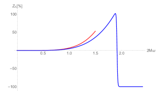
Figure 1: Amplification factor $Z_{\Lambda}$ (in percentage form) in Eq.(45) as a function of the frequency for the mode $s=\ell=m=2$, $a=0.999M$. The blue solid curve is our calculation using the MST method, explained in Sec.III.2. The red dashed curve is the approximation (i) mentioned in Sec.IV (i.e., approximation for $M\omega\ll 1$ and $\omega\ll\omega_{\text{SR}}$).

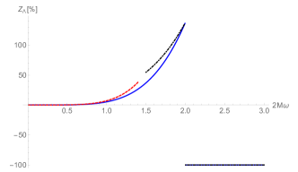
Figure 2: Amplification factor $Z_{\Lambda}$ (in percentage) in Eq.(45) in extremal Kerr as a function of the frequency. The mode is $s=\ell=m=2$, for which $2M\omega_{\text{SR}}=2$ and $\delta_{SR}^{2}>0$. The solid blue curve is our calculation using the MST method, Eq.(17). The red dashed curve is the approximation (i) mentioned in Sec.IV (i.e., approximation for $M\omega\ll 1$ and $\omega\ll\omega_{\text{SR}}$) with the choice $a=0.9999M$. The dashed black curve (which overlaps with the blue one for $M\omega>1$) corresponds to the asymptotics in Starobinskii and Churilov (1974) for $|\alpha|\ll m^{-4}\text{max}(1,|\alpha|^{2})$ for extremal Kerr.

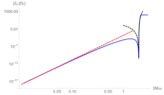
(a) $s=0,\ell=3,m=2$.

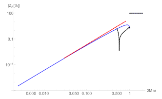
(b) $s=\ell=m=1$

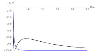
(c) $s=\ell=m=1$

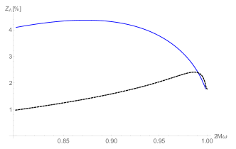
(d) $s=\ell=m=1$

Figure 3: Amplification factor $Z_{\Lambda}$ (in percentage) in extremal Kerr as a function of the frequency. Same colour and style coding for the curves as in Fig.2. Modes: (a) log-log plot for $s=0$, $\ell=3$, $m=2$, for which $2M\omega_{\text{SR}}=2$ and $\delta_{SR}^{2}<0$; (b) log-log plot for $s=\ell=m=1$, for which $2M\omega_{\text{SR}}=1$ and $\delta_{SR}^{2}>0$; (c) and (d) are linear and zoomed-in (near $k=0$, from the right and the left, respectively) versions of (b).

In this section we considered $\omega$ real; from now on we shall consider $\omega$ to be generally complex.

V Modes in near-extremal Kerr

In this section we turn to QNMs (Sec.V.1) and TRMs (Sec.V.2) in NEK and so we consider $\text{Im}(\omega)<0$ (we remind the reader that, in subextremal Kerr, no exponentially-unstable modes exist Whiting (1989), and so no poles of the Green function modes exist for $\text{Im}(\omega)>0$).

V.1 QNMs in NEK

In order to understand the limit to extremal Kerr, we describe in the first subsection the properties of QNMs in NEK which were derived in Detweiler (1980a); Mashhoon (1985); Hod (2008); Yang et al. (2013a, b); Zimmerman et al. (2015); Hod (2013); Leaver (1985). In the second subsection, we present our numerical calculation of these modes, showing agreement with results in the literature. This agreement validates our implementation of the MST and Nelder-Mead methods for calculating QNMs. We shall turn to QNMs in extremal Kerr in Sec.VII.1. We note that in that section we will find QNMs in the extremal case for mode parameters (namely, spin-2 field with $\ell=m=2$ and $3$) which the above analyses in NEK missed to find.

V.1.1 Properties of QNMs in NEK

It was shown in Yang et al. (2013a) that two families of QNMs branch off from the same family of QNMs as $a$ approaches extremality: zero-damping modes (ZDMs) and damped modes (DMs). As $a\to M$, the ZDM frequencies tend to $\omega_{\text{SR}}$, and so their imaginary part tends to zero, as their name suggests. The imaginary part of DM frequencies, on the other hand, tends to a finite value as $a\to M$. We next give some properties of these two families.

Let us start with the ZDMs. These modes are present for all values of $\ell$ and $m$. ZDMs are associated with the near-horizon geometry. For example, it can be shown that, in the eikonal limit $\ell\gg 1$, ZDMs reside on the extremum which the potential of the radial equation (obtained by suitably transforming the original Teukolsky equation to one with a real potential in the case of non-zero spin) possesses on the event horizon for all $\ell$ and $m$. The frequencies of ZDMs have the following asymptotics  Hod (2008); Yang et al. (2013a, b); Hod (2013) (which were partly based on, and corrected, an original derivation in Detweiler (1980a))

$$\omega_{\ell mn}\sim\omega_{\text{SR}}+2\pi T_{H}\left(m-\delta_{SR}-i\,\left(n+\frac{1}{2}\right)\right),\quad a\to M,$$ (46)

where $\delta_{SR}$ is taken to be the principal square root in Eq.(27) (so a positive number if $\delta_{SR}^{2}>0$ and with a positive imaginary part if $\delta_{SR}^{2}<0$) and $n=0,1,2,\dots$ Eq.(46) yields two slightly different behaviours for the leading order, as $a\to M$, of the imaginary part of the frequencies: it is “$-2\pi T_{H}(n+1/2)$” for the modes with $\delta_{SR}^{2}>0$, and it is even more negative for the modes with $\delta_{SR}^{2}<0$.

As $a\to M$, the temperature goes to zero and so the imaginary part of the frequencies in Eq.(46) goes to zero. The property that $\omega=\omega_{\text{SR}}$ is an accumulation point for the ZDM family of QNMs in the extremal limit was originally shown analytically in Detweiler (1980a) and corroborated numerically later in Leaver (1985). Despite it being an accumulation point for QNMs, which possess no incoming radiation (i.e., $B^{\text{inc}}_{\Lambda}=0$), the mode at $\omega=\omega_{\text{SR}}$ itself does possess incoming radiation (i.e., $B^{\text{inc}}_{\Lambda}\neq 0$) in extremal Kerr. This can be seen from a basic conservation-of-energy argument which, in fact, also applies to all real-frequency non-superradiant modes in either extremal or sub-extremal Kerr Detweiler and Ipser (1973); Teukolsky and Press (1974); Casals et al. (2016b). In sub-extremal Kerr, this result has been extended to the superradiant regime: the only mode with $\omega\in\mathbb{R}$ and no incoming radiation is the trivial mode Andersson et al. (2017). This then implies the non-existence of exponentially-growing modes in sub-extremal Kerr Andersson et al. (2017); Hartle and Wilkins (1974), a result which had been previously proven in Whiting (1989) in a different way.

The accumulation of ZDMs near the superradiant bound frequency leads to certain physical features. Away from the horizon, it leads to a temporary power-law decay of the field at early times Glampedakis and Andersson (2001); Yang et al. (2013b), which then gives way to the characteristic QNM exponential decay, before ending up in a power-law decay due to the origin BC Price (1972). Near the horizon, the accummulation of ZDMs leads to a transient growth of the field Gralla et al. (2016b). Also, this accummulation leads to a distinct observational feature in the gravitational waveform in a near-horizon inspiral Gralla et al. (2016a); Comp re et al. (2018), as we mentioned in the Introduction.

Let us now turn to DMs. Although we are not aware of an actual proof, the exact calculations in the literature and in this paper seem to suggest that DMs satisfy the following properties:

• they have $|\text{Re}(\omega_{\ell mn})|>|\omega_{\text{SR}}|$;

• they originate from lower overtones within the family of QNMs at smaller $a$.

Refs. Mashhoon (1985); Yang et al. (2013b) obtained large-$\ell$ WKB asymptotics for the values of the frequencies of DMs. In this eikonal limit, it has been shown that DMs reside near the maximum of the radial potential outside the horizon, whenever such a maximum exists. Still in the eikonal limit, the condition for the existence of such a maximum and, equivalently, for the existence of DMs, is $\mu<\mu_{c}$, where $\mu\equiv|m|/(\ell+1/2)$ and $\mu_{c}\approx 0.74$. For general $\ell$ and $m$, the condition for the existence of a maximum outside the horizon is

$$\mathcal{F}_{s}^{2}\equiv\delta_{SR}^{2}+1/4<0.$$ (47)

Refs.Yang et al. (2013a, b) thus suggest that, in general, DMs are present if and only if Eq.(47) is satisfied. On the other hand, Fig.3 in Cook (2014) shows that for $-s=\ell=m=2$ there is a QNM with finite imaginary part, even though it satisfies $\mathcal{F}_{s}^{2}>0$, as can be readily checked. This QNM possesses the properties opposite to (i) and (ii) above. Furthermore, this QNM is not the only one with finite imaginary part for which Eq.(47) is not satisfied, and which has the property opposite to, at least, (i) above – we shall see in Sec. VII.1 that is the case in extremal Kerr for $s=-2$ and $\ell=m=3$. Therefore, from the exact calculations in the literature and in this paper, it seems that there exist QNMs with negative imaginary part always when Eq.(47) is satisfied, and also, at least in some cases, when Eq.(47) is not satisfied. In this paper, we shall continue to refer to the former ones (i.e., those that necessarily exist when $\mathcal{F}_{s}^{2}<0$) as DMs and we shall refer to the latter ones (i.e., those which may exist when $\mathcal{F}_{s}^{2}>0$) as “non-standard DMs” (NSDM) . It also seems (although we are not aware of an actual proof) that DMs satisfy properties (i) and (ii) above whereas NSDMs satisfy the opposite properties.

We note that for $m<0$ and $\text{Re}(\omega)>0$ – or, equivalently, for $m>0$ and $\text{Re}(\omega)<0$, by virtue of the symmetry (28) – there exist the standard QNMs, with a finite imaginary part but without being “partnered up with” ZDMs (i.e., these standard QNMs and the ZDMs did not branch off from the same family of modes at smaller $a$).

We finish this subsection by relating various conditions which we have mentioned. Firstly, it has been checked numerically that $\delta_{SR}^{2}<0\leftrightarrow\mathcal{F}_{s}^{2}<0$. This has been checked for a large set of modes with $s=0$ and “$-2$” in Yang et al. (2013a, b) and for a set of modes with $|s|=0$, $1$ and $2$ by us. Secondly, Yang et al. (2013a, b) show that the equivalence $\mu<\mu_{c}\leftrightarrow\mathcal{F}_{s}^{2}<0$ holds for most modes that they checked with $s=0$ and “$-2$” but does not hold for a few modes. Similarly, we checked that, for $|s|=1$, the equivalence $\mu<\mu_{c}\leftrightarrow\mathcal{F}_{s}^{2}<0$ holds for most modes but does not hold for some modes (such as $\ell=m=1$ and $\ell=13$, $m=10$). Finally, we note that $\mathcal{F}_{s}^{2}<0$ is equivalent to $\nu_{c}(\nu_{c}+1)>0$. That is, DMs exist if and only if the eigenvalue of the Casimir operator of the $\mathfrak{sl}(2,\mathbb{R})$ in NHEK is positive (although NSDMs may exist even if it is non-positive).

V.1.2 Calculation of QNMs in NEK

Let us now turn to our calculation of QNMs in NEK. The contourplots of the Wronskian factor (30) (to be precise, of $\log_{10}|W_{\Lambda}^{f}|$) in Fig.4 shows the accumulation of ZDMs near $\omega=\omega_{\text{SR}}$. The only case with $\mathcal{F}_{s}^{2}>0$ in that figure is that in Fig.4(c). In this case, within the analyzed region of the complex plane, we found no DMs – as expected – and no NSDMs. The top two plots correspond to plots in Fig.7 in Yang et al. (2013b) (Fig.4(c) has a slightly larger value of $a$ than a plot in Fig.7 in Yang et al. (2013b)).

We note that Fig.7 in Yang et al. (2013b) shows contour plots of Leaver’s continued fraction. Apart from the QNMs, their plots show poles in the continued fraction, which can be “very close” to the QNMs. In our Fig.4, on the other hand, we plot the Wronskian factor $W_{\Lambda}^{f}$ and it does not display poles near the QNM frequencies. This is due to having defined $W_{\Lambda}^{f}$ in Eq.(30) by removing a $\Gamma$-factor in $W_{\Lambda}$ which, as it seems, contains its poles – see Secs.III.2 and V.2. This can be seen as an advantage of our approach, since the poles in Leaver’s continued fraction become arbitrarily close to $\omega_{\ell mn}$, as can be observed at the bottom left panel of Fig.7 Yang et al. (2013b). The presence of these poles in Leaver’s continued fraction may lead to numerical issues when approaching the extremal limit.

In Appendix B we tabulate various QNM frequencies in NEK. We calculated these QNMs to 16 digits of precision using the method described in Sec.III. Fig. 4 shows these NEK QNMs . Our NEK QNM values for $s=-2$, $\ell=2$ agree with those in QNM to the following typical number of digits of precision: 7 (worst was 4 digits) for $m=2$; 10 (worst was 7 digits) for $m=1$; 5 (worst was 3 digits) for $m=0$. As stated in QNM , however, the QNM values contained there are unreliable in NEK (“roughly, when $a/M\geq 0.999$”), where no error bars are given. We note that, for the cases that we calculated the QNMs for, Ref. QNM seems to provide values only for DMs. The exception to that is the case where no DMs exist, which is that in Table 2, for which QNM does provide the ZDM values. In our App.B, on the other hand, we provide DMs as well as ZDMs for all cases where they exist.

For $m=0$ we noticed that the values of the real part of the ZDM frequencies were below the precision we used in the calculation every time as we increased that precision (to even 32 digits). We thus do not provide these values in the $m=0$ Table 3.

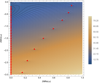
(a) $s=-2,\ell=2,m=0,a=0.998M$

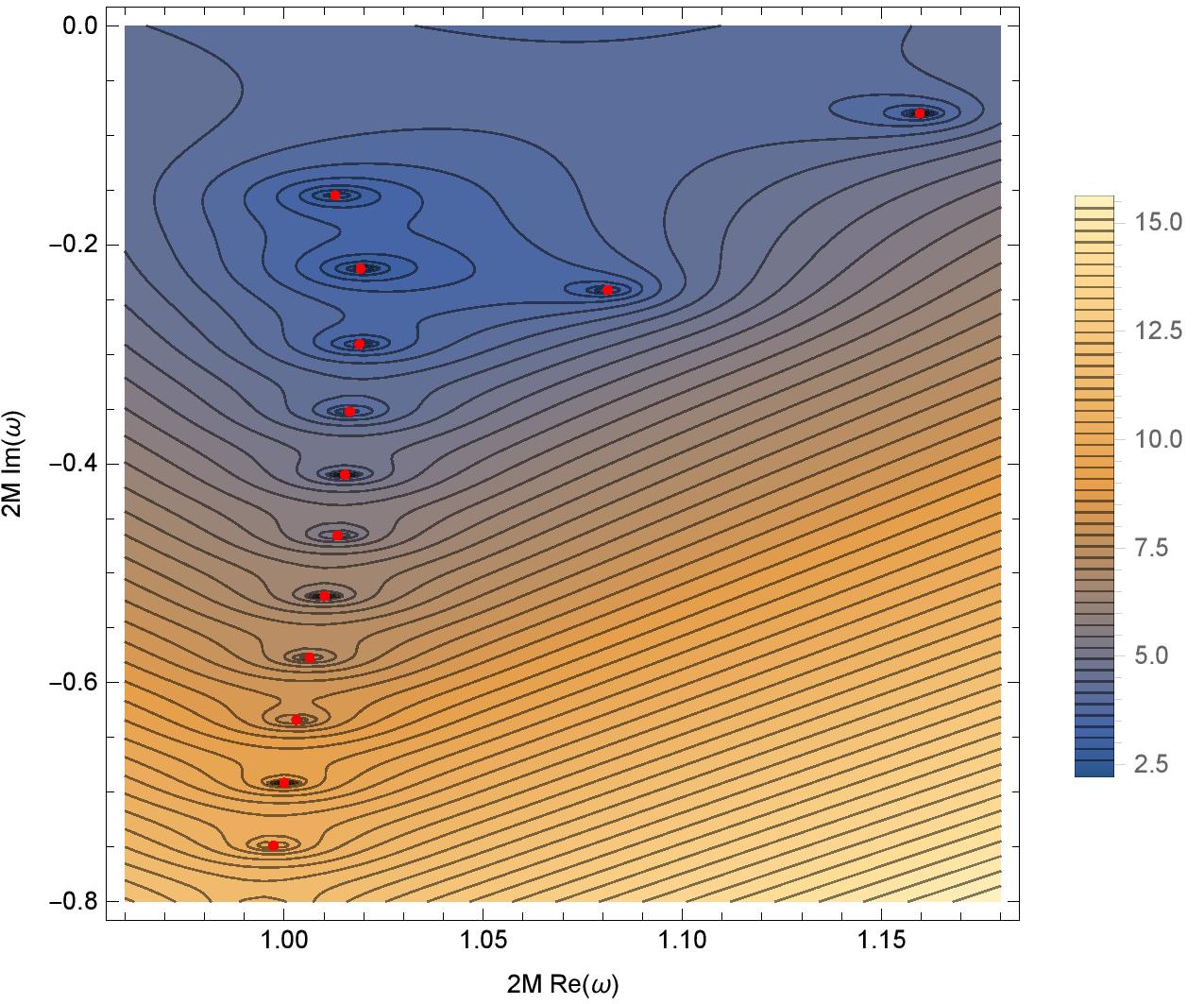
(b) $s=-2,\ell=2,m=1,a=0.998M$

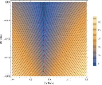
(c) $s=-2,\ell=2,m=,a=0.9999M$

Figure 4: Contour plots of $\log_{10}|W_{\Lambda}^{f}|$ in NEK for $s=-2$, $\ell=2$ and $m=0,1,2$. The superradiant bound frequencies for these modes are $2M\omega_{\text{SR}}=0$ (for $m=0$), $\approx 0.938$ (for $m=1$) and $\approx 1.972$ (for $m=2$). The QNMs in Tables 2– 5 are indicated with red dots. N.B.: the top two plots correspond to Fig.7 in Yang et al. (2013b).

V.2 TRMs in NEK

Apart from the QNMs, there is another interesting set of modes worth considering. Totally reflected modes (TRMs) correspond, physically, to waves with no transmission and, mathematically, to a singularity in both $\mathcal{B}^{\text{inc}}_{\Lambda}$ and $\mathcal{B}^{\text{ref}}_{\Lambda}$ while $\mathcal{B}^{\text{inc}}_{\Lambda}/\mathcal{B}^{\text{ref}}_{\Lambda}$ is finite. Therefore, the Wronskian is singular at a TRM frequency.

Ref.Keshet and Neitzke (2008) derived the following exact expression for TRM frequencies in sub-extremal Kerr

$$\omega=\omega_{\text{SR}}-2\pi iT_{H}(n-s+1),$$ (48)

where $n=0,1,2,\dots$ These frequencies coincide with the poles of the factor $\Gamma(1-s-2i\epsilon_{+})$ in Eq.(30), which we removed from the Wronskian precisely with the intention of avoiding its poles. Note that the difference between the TRMs and the QNMs, which asympote as in (46), is only to higher order in the asymptotics (for the specific case of $m=0$ in NEK, this had already been noticed in Hod (2013)). Fig.6 shows that the TRMs and QNMs are coming closer together as we increase the value of $a$. When $a=M$ an infinite amount of both types of modes accumulate and mix in such a way that a finite discontinuity (BC) is formed. We investigate this feature in the next section.

VI Branch cuts

In this section we first investigate the presence of BCs in the complex frequency plane and afterwards the formation of the superradiant BC.

VI.1 Search for branch cuts

In order to start the investigation of the presence of BCs we plot both the absolute value and the phase of the Wronskian when taking a loop around a certain frequency. That is, we calculated the Wronskian for $\omega=\omega_{0}+Re^{i\phi}$, given some frequency $\omega_{0}\in\mathbb{C}$, radius $R>0$ away from it, and varying the phase $\phi:0\to 2\pi$. The discontinuity of the Wronskian at some $\phi$ would indicate a BC, possibly stemming from $\omega_{0}$ (branch point).

We performed such loops in many instances. For example, in Fig.5 we plot the Wronskian for $s=\ell=m=2$ in subextremal Kerr when going around the origin: $\omega_{0}=0$ and $R=1/M=2$. For this mode, the superradiant bound frequency is $M\omega_{\text{SR}}\approx 0.2679$ and the particular Hartle-Wilkins frequency (see App.A.1) is $M\omega_{HW}\approx 0.2679+0.2320i$. Therefore both of these frequencies lie inside the circle that we take around the origin. The only discontinuity that we find is near (or at) the phase $\phi=3\pi/2$. This discontinuity corresponds to the well-known BC from $\omega=0$ down the negative imaginary axis  Leaver (1986a); Hod (2000); Casals et al. (2016a) . We also note that somewhere in the fourth quadrant there is a steep structure (though not an actual discontinuity), which will result in the superradiant BC in the extremal limit. We also did similar plots of the Wronskian around the origin for other modes and we found the same qualitative features: (i) there is a BC down from $\omega=0$; (ii) there is an indication that an extra BC from $\omega_{\text{SR}}$ is forming as $a$ approaches $M$.

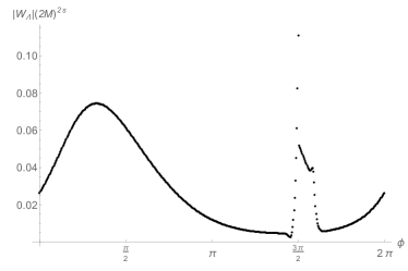
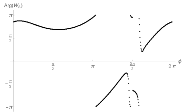
Figure 5: Plot of the absolute value (top) and argument (bottom) of $\mathcal{W}_{\Lambda}$ for $s=\ell=m=2$ and $a=0.5M$ on a loop $\omega=e^{i\phi}/M$ around the origin, which encircles $M\omega_{\text{SR}}\approx 0.2679$ and $M\omega_{HW}\approx 0.2679+0.2320i$. There is a discontinuity near (or at) $\phi=3\pi/2$, corresponding to the well-known BC down from the origin. A steep structure is seen in the fourth quadrant, which is related to the formation of the superradiant BC in the extremal case.

We carried out a similar search for BCs in the extremal case. We found BCs down from $\omega=0$ and $\omega=\omega_{\text{SR}}$ and no other BCs. We anticipated the existence of the BC down from $\omega=\omega_{\text{SR}}$ in Sec.II. In the next subsection we show how this BC is formed.

VI.2 Formation of superradiant BC

Using asymptotics for the QNMs as $a\to M$, indications were found in Detweiler (1980a); Glampedakis and Andersson (2001) that the ZDMs in NEK accumulate towards the superradiant bound frequency so as to try to form a new BC down from $\omega=\omega_{\text{SR}}$. We already saw this accumulation of ZDMs in Fig.4.

The above indication of formation of a superradiant BC is illustrated more clearly in the 3D plots of the absolute value of the Wronskian in Fig.6, where we increase $a=0.95M\to 0.99M\to M$. Fig.6 clearly shows how, in NEK, a series of TRMs (i.e., poles of the Wronskian) appear near a series of ZDMs (which are QNMs, i.e., zeros of the Wronskian), thus yielding a steep structure in the numerically-calculated Wronskian. We already spotted this steep structure in the fourth quadrant in Fig. 5. As $a$ increases, the series of TRMs and the series of ZDMs are seen to approach each other, in agreement with Eqs.(46) and (48). This approach ends up yielding a BC discontinuity stemming from the (branch) point $\omega=\omega_{\text{SR}}$ in the actual limit $a=M$.

This superradiant BC in extremal Kerr can be seen in Figs.7, 9 and 10, which contain a contourplot version of Fig.6c as well as similar contourplots of the absolute value of the Wronskian for other modes. The superradiant BC is also manifest in the phase of the Wronskian in extremal Kerr as shown in Fig.8 for a sample of modes. The BC is clear in Fig.8a for $m=2$; in Fig.8b for $m=0$ the BC can be readily inferred from the symmetry (33); Fig.8c for $m=-1$ has no BC for $\text{Re}(\omega)>0$ but we include it for completeness. With red dots we indicate the QNM frequencies. One may see that the variation of the values of the phase along a loop around a QNM is precisely that corresponding to a simple zero of $W_{\Lambda}$, and so to a simple pole of $1/W_{\Lambda}$, ie, a QNM. We investigate poles in extremal Kerr in the next section.

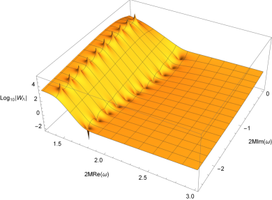
(a) $s=0,\ell=3,m=2,a=0.95M$

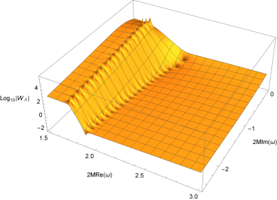
(b) $s=0,\ell=3,m=2,a=0.99M$

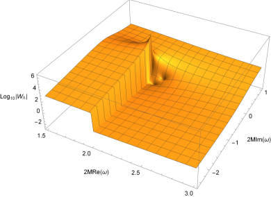
(c) $s=0,\ell=3,m=2,a=M$

Figure 6: Plots of $\log_{10}\left|\mathcal{W}_{\Lambda}\right|$ for $a=0.95M$ and $0.99M$ and of $\log_{10}\left|W_{\Lambda}\right|$ (so for $a=M$). The mode is $s=0,\ell=3,m=2$, for which it is $2M\omega_{\text{SR}}\approx$ 1.447 (for $a=0.95M$), $\approx$1.735 (for $a=0.99M$), =2 (for $a=M$).

VII QNMs and search for unstable modes in extremal Kerr

In this section we investigate poles of the Green function modes (i.e., zeros of the Wronskian) in extremal Kerr. These poles may correspond to either QNMs (if they lie in the lower complex-frequency half-plane) or to exponentially-unstable modes (if they lie in the upper half-plane).

VII.1 QNMs in extremal Kerr

We here turn to the QNMs in extremal Kerr. The condition in Eq.(47) (which was given for NEK but carries over to extremal Kerr) differentiates between two different regimes: presence of DMs when $\mathcal{F}_{s}^{2}<0$; absence of DMs when $\mathcal{F}_{s}^{2}>0$. As indicated in Sec.V.1.1, however, there may exist NSDMs when $\mathcal{F}_{s}^{2}>0$.

In Figs.7, 9, 10 and 11 we plot the absolute value of the full Wronskian (9) in the complex-frequency plane for $m\geq 0$. In Fig.7a we can see, for $s=0$ and $\ell=m=2$, for which $\mathcal{F}_{s}^{2}<0$, two isolated QNMs frequencies appearing to the right of the BC, which correspond to DMs. In Fig.7b for $s=\ell=m=1$, for which $\mathcal{F}_{s}^{2}>0$, there are no DMs nor, within the analyzed region, NSDMs.

In Figs.9 we investigate the modes $\ell=2$ and $0\leq m\leq 2$ for $s=-2$. It is $\mathcal{F}_{s}^{2}<0$ for $m=0$, $1$ and $\mathcal{F}_{s}^{2}>0$ for $m=2$. Correspondingly, we observe DMs (again to the right of the BC, i.e., satisying property (i) in Sec.V.1.1) for $m=0$, $1$ and no DMs for $m=2$ in the analyzed region of the complex-$\omega$ plane. In the case $m=2$, however, we do observe a NSDM, which is just the extremal limit of the corresponding ($n=5$) QNM in Fig.3 in Cook (2014). For $m=0$ there is an accumulation of QNMs at $\omega=\omega_{\text{SR}}=0$ in NEK (see Fig.4a), leading to a BC along the negative imaginary axis for the phase (but not the absolute value, as noted in footnote 11) of the Wronskian in extremal Kerr (Fig.8b). For $m=1$ we can see a BC that is formed from the accumulation in NEK of QNMs and TRMs - see Sec.V.2.

The previous plots are contour plots. In Fig.11 we plot the cases in Fig.9 as 3-D plots instead. These show not only the cut and DM structure but also the behaviour of the Wronskian as $k\to 0$: zero for $m=1$ and $2$ and divergent for $m=0$. The vanishing for $m=1$ and $2$ is in agreement with Eq.(41), since it is $s=-2$ and, respectively, $\nu_{c}\approx 1.42$ and $-1/2+2.05i$ for these modes. The divergence for $m=0$ is clearly in agreement with Eq.(43). Similarly, Fig.6c shows that the Wronskian diverges as $k\to 0$ in this case, also in agreement with Eq.(41), since it is $s=0$ and $\nu_{c}\approx 1.71$.

Another mode for which we observe a NSDM is the case $s=-2$, $\ell=m=3$ which we plot in Fig.10. This is a mode with $\mathcal{F}_{s}^{2}>0$ and it lies to the left of the BC (i.e., the opposite of property (i) in Sec.V.1.1).

In Fig.12 we deal with the distinct case of negative $m$: modes for $s=\ell=2$ and $m=-1$ and $-2$. In these cases and for $\text{Re}(\omega)>0$, there are no BCs (their superradiant BCs stem from $\omega_{\text{SR}}<0$) and there are the “standard” QNMs. The QNMs in this figure are to be compared with the corresponding ones in Fig.3 in Leaver (1985) – visual agreement is found.

In Appendix C we tabulate various QNM frequencies in extremal Kerr, calculated using the MST method of Sec.III to 16 digits of precision. These extremal Kerr QNMs are to be compared with the data in Richartz (2016). Our extremal Kerr QNM values agree with those in Richartz (2016) to all digits of precision given in Richartz (2016); the frequencies in Richartz (2016) are given up to a maximum of 7 digits of precision, whereas we give them up to 16. We note that Richartz (2016) only provides QNMs for overtones $n=0$ and $1$, whereas in App.C we provide new QNM values up to higher overtones (up to $n=6$). Importantly, we give the value for the most astrophysically relevant $s=-2$ QNM: $\ell=m=2$ in table 9, as well as for $\ell=m=3$ in table 12, neither of which was previously given in the literature, to the best of our knowledge.

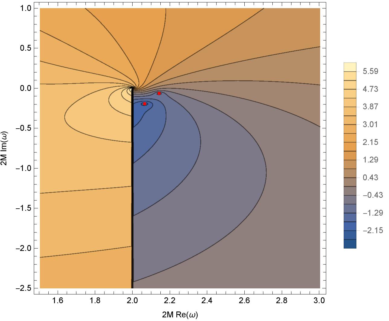
(a) $s=0,\ell=3,m=2,a=M$

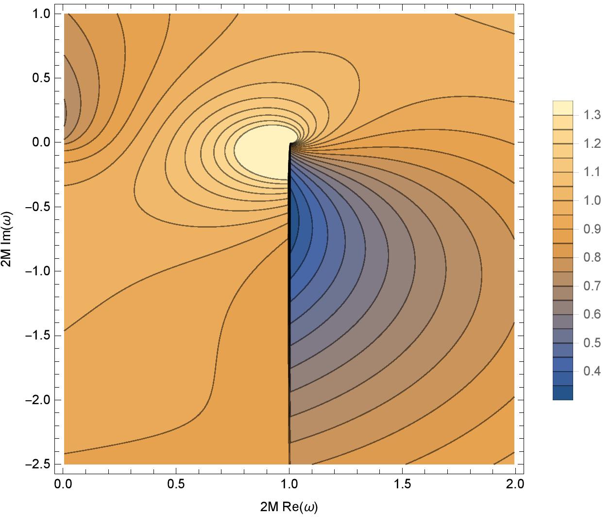
(b) $s=\ell=m=1$, $a=M$

Figure 7: Contour plots of $\log_{10}\left|\left(2M\right)^{2s}W_{\Lambda}\right|$ in the complex-frequency plane in extremal Kerr. The modes are: (a) $s=0,\ell=3,m=2$, for which $2M\omega_{\text{SR}}=2$ and $\mathcal{F}_{s}^{2}<0$, in agreement with the presence of DMs which we observe (two to the right of the BC), and (b) $s=\ell=m=1$, for which $2M\omega_{\text{SR}}=1$ and $\mathcal{F}_{s}^{2}>0$, in agreement with the absence of DMs which we observe. The QNMs in Table 6 are indicated with red dots.

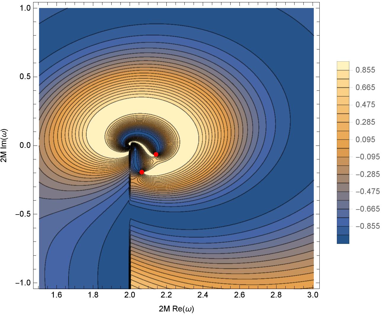
(a) $s=0,\ell=3,m=2,a=M$

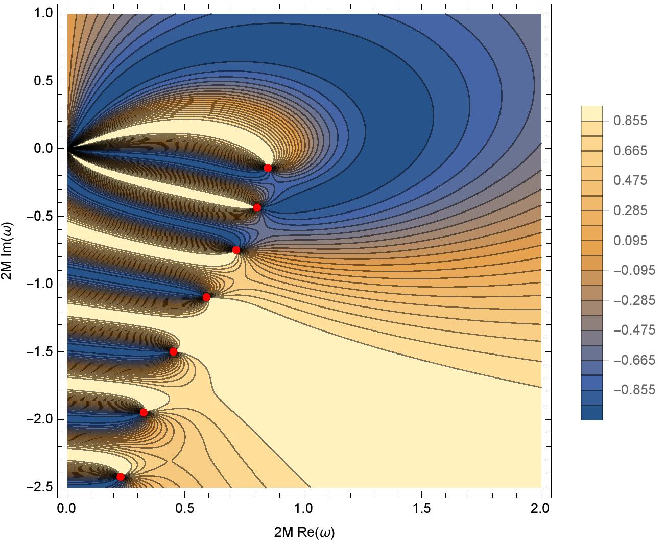
(b) $s=-2,\ell=2,m=0,a=M$

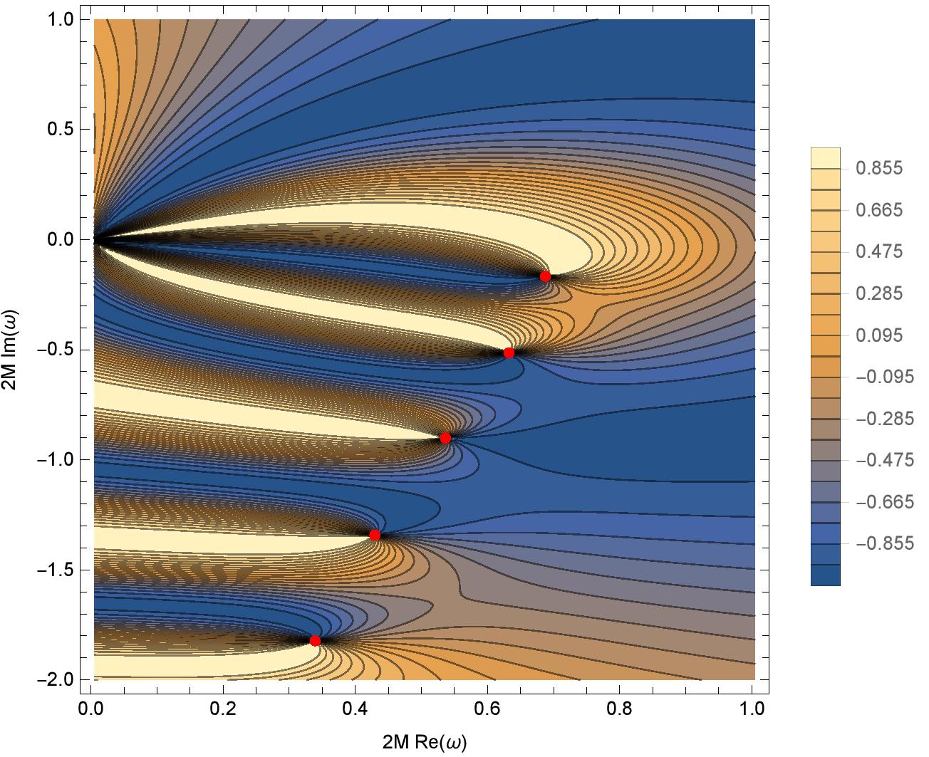
(c) $s=-2,\ell=2,m=-1,a=M$

Figure 8: Contour plots of $\sin\left(\arg\left(W_{\Lambda}\right)\right)$ in the complex-$\omega$ plane in extremal Kerr. The QNMs in Tables 6, 7 and 10 are indicated with red dots.

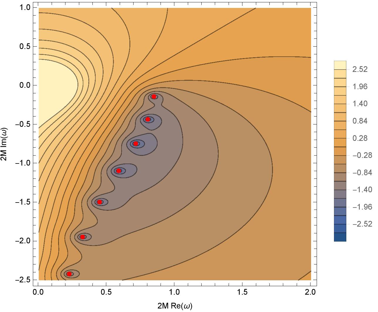
(a) $s=-2,\ell=2,m=0,a=M$

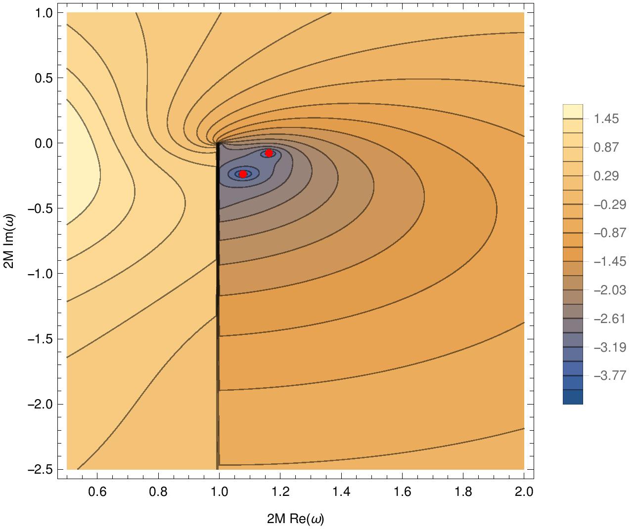
(b) $s=-2,\ell=2,m=1,a=M$

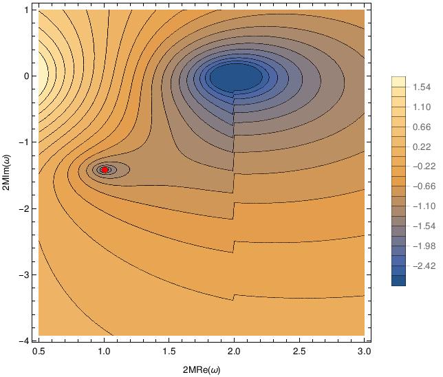
(c) $s=-2,\ell=2,m=2,a=M$

Figure 9: Contour plot of $\log_{10}\left|\left(2M\right)^{2s}W_{\Lambda}\right|$ in the complex-$\omega$ plane in extremal Kerr for $s=-2$, $\ell=2$, $m=0$, $1$ and $2$. For $m=0$ and $1$ it is $\mathcal{F}_{s}^{2}<0$ and so DMs appear. For $m=2$ it is $\mathcal{F}_{s}^{2}>0$ and so DMs do not appear but a NSDM  does appear. The QNMs in Tables 7, 8 and 9 are indicated with red dots.

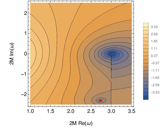
Figure 10: Contour plot of $\log_{10}\left|\left(2M\right)^{2s}W_{\Lambda}\right|$ in the complex-$\omega$ plane for $s=-2$, $\ell=m=3$ in extremal Kerr. It is $\mathcal{F}_{s}^{2}>0$ and so DMs do not appear, but there is the presence of a NSDM. The QNM in Table 12 is indicated with a red dot.

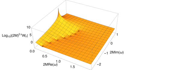
(a) $s=-2,\ell=2,m=0,a=M$

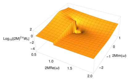
(b) $s=-2,\ell=2,m=1,a=M$

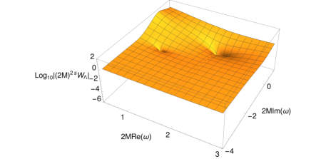
(c) $s=-2,\ell=2,m=2,a=M$

Figure 11: These are 3-D versions of the plots in Fig.9.

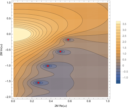
(a) $s=-2,\ell=2,m=-2,a=M$

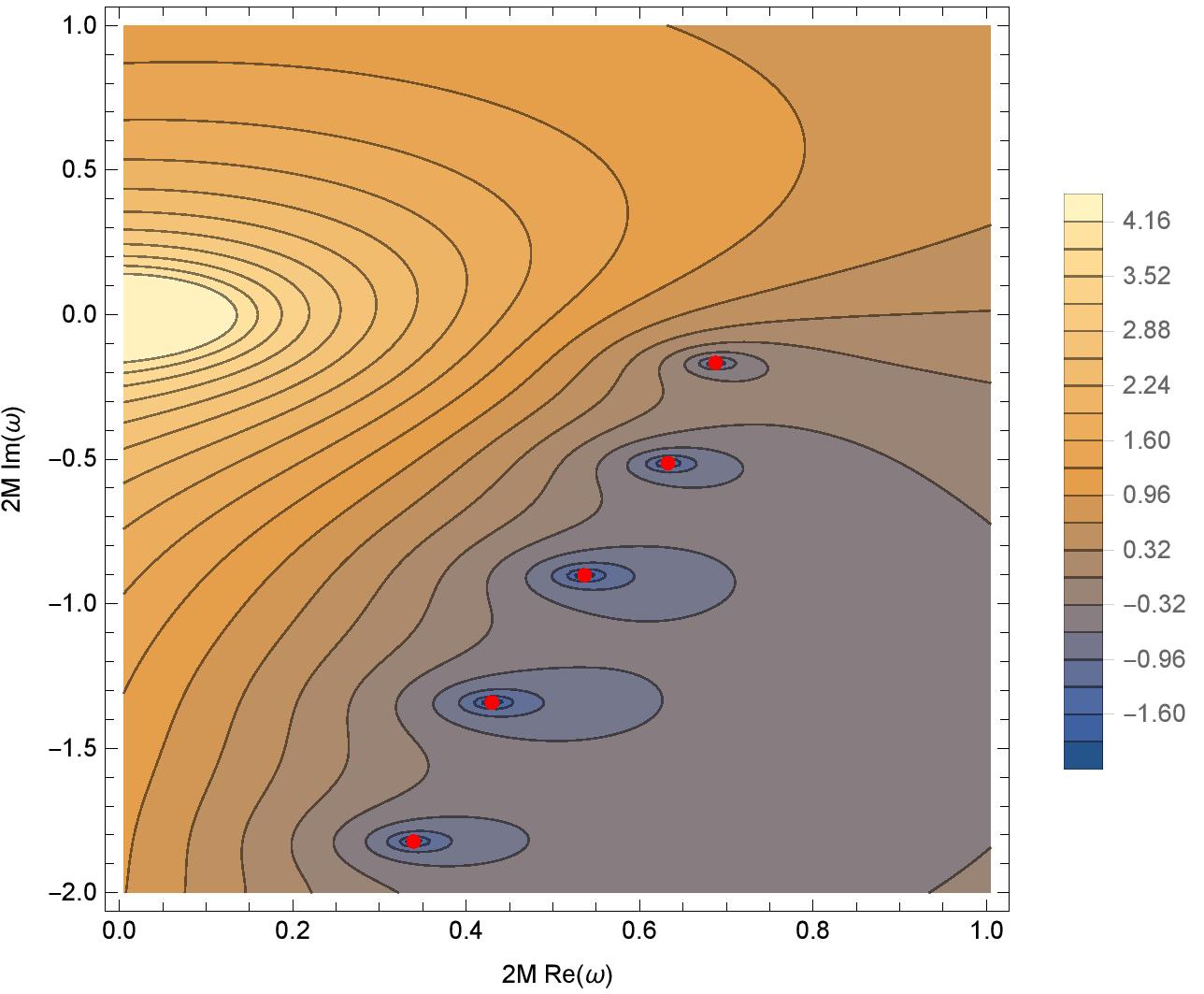
(b) $s=-2,\ell=2,m=-1,a=M$

Figure 12: Contour plots of $\log_{10}\left|\left(2M\right)^{2s}W_{\Lambda}\right|$ in the complex-frequency plane in extremal Kerr for $s=-2$, $\ell=2$ and $m=-1,-2$. The QNMs in Tables 10 and 11 are indicated with red dots. Cf. Fig.3 in Leaver (1985).

VII.2 Search for unstable modes

If the modes of the retarded Green function possessed a singularity on the upper frequency half-plane, that would indicate a linear instability of the space-time Detweiler and Ipser (1973). In principle, such a singularity could be a branch point or a pole (i.e., a mode with no incoming radiation).

Detweiler Detweiler and Ipser (1973) showed that there exist no modes with no incoming radiation in the upper plane in the case of scalar perturbations of extremal Kerr. Later, Aretakis Aretakis (2012) proved the decay of the full scalar field in the axisymmetric case on and outside the horizon;  Dain and de Austria (2015) proved similarly for axisymmetric gravitational perturbations outside the horizon. On the horizon, it has been shown in Casals et al. (2016b); Gralla and Zimmerman (2018) that the branch point on the superradiant bound frequency leads to the so-called Aretakis phenomenon Aretakis (2015, 2011). In its turn, the branch point at the origin leads to a late-time decay in the field Casals and Zimmerman (2018), as otherwise expected. It therefore seems that it has not been proven that the Green function modes with $m\neq 0$ do not possess singularities in the upper complex-frequency plane.

For scalar perturbations and $a\leq M$, Ref.Detweiler and Ipser (1973) gives bounds on the real and imaginary parts of the frequencies of potential modes in the upper plane possessing no incoming radiation. In particular, the real part should lie within the superradiant regime . Ref. Richartz (2016) and, in the case of scalar perturbartions, also Detweiler and Ipser (1973), numerically looked for modes with no incoming radiation in the upper plane of extremal Kerr and could not find any. Here, we report that we also looked for modes with no incoming radiation in the upper plane of extremal Kerr and did not find any, thus confirming the results in Detweiler and Ipser (1973); Richartz (2016). Examples of the search are the already mentioned Figs.7–12, where we went up to $2M\text{Im}(\omega)=1$. These figures also show that there are no “physical” branch points in the upper plane for these modes, thus complementing the investigation in Sec.VI.1.

Finally, we note that the result in Andersson et al. (2017) that no poles can lie on the real axis for $a<M$ together with the fact that there cannot be a pole at the branch point $\omega_{\text{SR}}$ Casals et al. (2016b); Richartz et al. (2017) provides an argument – although not a rigorous proof – that no poles cross the real axis as $a$ increases from $0$ to $M$ and so for the absence of poles in the upper plane in extremal Kerr.

VIII Conclusions

We have carried out a thorough spectroscopic investigation in extremal Kerr space-time as well as in near-extremal Kerr. We have calculated the superradiant amplification factor and quasi-normal modes and shown the formation of the extra superradiant branch cut. Our results provide a corroboration of the MST method developed in Casals and Zimmerman (2018) and of the results in Richartz (2016). Our tabulated values for quasi-normal mode frequencies signify an extension in both the accuracy and in the type of modes tabulated in the literature (Richartz (2016) for extremal Kerr and QNM for near-extremal Kerr), including the astrophysically-relevant quasi-normal mode for $-s=\ell=m=2$ in Table 12. Furthermore, we searched for both poles and branch points in the upper frequency plane in extremal Kerr and report that we did not find any, providing further support for the mode stability of extremal Kerr off the horizon. We also gave an argument for the absence of such poles.

A seemingly open issue is finding a condition for existence of quasi-normal modes with a finite imaginary part in (near-)extremal Kerr as well as determining the number of such modes. In particular, the condition Eq.(47) misses quasi-normal modes with a finite imaginary part (the ones which we have called non-standard damped modes), as seen for the particular cases of $s=-2$ modes with $\ell=m=2$ and $3$. On the other hand, we have found no quasi-normal modes for $s=\ell=m=1$ within the large region in the complex plane which we have considered, although of course that is no proof that there exists no mode outside that region.

In terms of astrophysics, it will be interesting to obtain, in the future, the gravitational waveform due to a particle inspiraling into an extremal Kerr black hole, and compare it to the results in Gralla et al. (2016a) for a near-extremal black hole and to the results in the near-horizon extremal Kerr geometry Porfyriadis and Strominger (2014).

Appendix A Special frequencies

In this appendix we investigate various specific frequencies. In Sec.A.1 we give evidence that a certain frequency suggested in Hartle and Wilkins (1974) to be a branch point is actually not a branch point; in Sec.A.2 we give evidence that certain frequencies suggested in Hod (2015, 2016) to be QNMs are actually not QNMs; in Sec.A.3 we investigate the so-called algebraically-special frequencies.

A.1 Hartle-Wilkins frequency

Hartle and Wilkins Hartle and Wilkins (1974) observed that it was possible that the frequency

$$\omega_{HW}=\omega_{\text{SR}}+i(s-1)\dfrac{r_{+}-M}{2Mr_{+}}$$ (49)

is a branch point. Interestingly, such frequency would lie in the upper-half complex-$\omega$ plane for $s=2$ and, in that case, it might lead to an instability of the black hole. We have calculated the Wronskian for $s=\ell=m=2$ and the token value of $a=0.5M$ when going around this frequency: $\omega_{0}=\omega_{HW}$ and $R=|\omega_{HW}|/5$. We observed no discontinuity in $|\mathcal{W}_{\Lambda}|$ nor in $\arg(\mathcal{W}_{\Lambda})$, thus providing strong evidence that the Hartle-Wilkins frequency is not a branch point at least for this mode.

A.2 Hod frequencies

In Sec.V.1.1 we gave the generally accepted picture of DMs and ZDMs. However, it was argued by Hod Hod (2015, 2016) (based on the analysis in Detweiler (1980a)) that DMs also exist for $\mu\geq\mu_{c}$ as long as $a$ is sufficiently close to $M$. For example, for $s=\ell=m=2$, Hod (2015) predicts DMs at

$$\omega\approx\omega_{\text{SR}}+\left(0.324-0.07i\right)e^{-1.532n},$$ (50)

where $n\in\mathbb{Z}^{+}$. However, Refs. Zimmerman et al. (2015) and Richartz (2016), carried out a numerical search for these DMs in, respectively, NEK and extremal Kerr, and did not find any. Similarly, we carried out a numerical search in extremal Kerr for these DMs for $n=2$ using a grid of stepsize $\Delta\omega_{r}=\Delta\omega_{i}=10^{-6}$ along the directions of both the real and imaginary parts of the frequency and we also found no evidence of the presence of such DMs.

A.3 Algebraically-special Frequencies

Gravitational ($|s|=2$) perturbations of black holes admit frequencies for which the radial solution for spin $s$ (either $s=+2$ or $s=-2$) is the trivial solution whereas the radial solution for spin “$-s$” is a non-trivial solution. These frequencies are the so-called algebraically-special (AS) frequencies Wald (1973); Chandrasekhar (1984).

The AS frequencies satisfy the following equation Chandrasekhar (1984); Maassen van den Brink (2000):

$$\lambdabar^{2}\left(\lambdabar+2\right)^{2}+8\lambdabar\left(5\lambdabar\left(am\omega-a^{2}\omega^{2}\right)+6\left(am\omega+a^{2}\omega^{2}\right)\right)+$$

$$36\omega^{2}+144\left(am\omega-a^{2}\omega^{2}\right)^{2}=0,$$ (51)

where $\lambdabar\equiv\left.\lambda_{\Lambda}\right|_{s=-2}$. The left-hand side of Eq.(A.3) is the so-called Teukolsky-Starobinsky constant, which serves to relate (radial and angular) solutions for spin $s$ to solutions with spin “$-s$”.

The radial solutions at AS frequencies can be found in closed form Chandrasekhar (1984) and, for $a>0$, they correspond to totally transmitted modes (TTMs), i.e., modes with zero reflection coefficient Maassen van den Brink (2000). For $a=0$, the AS frequencies are given by “$-i(\ell-1)(\ell+2)\left((\ell-1)(\ell+2)+2\right)/6$”  Maassen van den Brink (2000). As $a$ increases, not only the AS frequencies move away from the negative imaginary axis for $m\neq 0$ but also a family of QNMs stems off from the AS frequency at $a=0$ Maassen van den Brink (2000).

Here we solve Eq.(A.3) numerically and plot the result in Fig.13. From Eq.(31) it follows that the AS frequency for “$-m$” is equal to that for “$+m$” after changing the sign of its real part, as reflected in Fig.13. The case for $\ell=2$ was already plotted in Fig.7 Onozawa (1997), with which our Fig.13 agrees. We also compare the numerical values of the AS frequencies with the small $a/M$ expansion in Eq.7.26 Maassen van den Brink (2000), and here we give the values of the AS frequencies for extremal Kerr for $s=-2$, $\ell=2$ and $m=\pm 2$: $2M\omega\approx\pm 1.26369-1.14328i$.

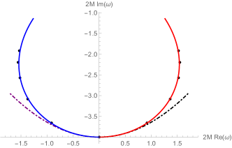
Figure 13: Algebraically-special frequencies for $\ell=2$ and $m=+2$ (red) and $m=-2$ (blue). The solid curves are our values for the roots of Eq.(A.3) (as $a$ increases, the value of the imaginary part becomes less negative); the black dots are the AS frequencies in Table A.1 in Chandrasekhar (1984) (N.B.: for $a=0.3M$ and $m=-2$ we changed the sign of the imaginary part of the frequency in Chandrasekhar (1984)); the dashed curves correspond to Eq.7.27 Maassen van den Brink (2000). At $a=0$ the AS frequency is “$-4i$” and as $a$ increases the AS frequencies move away from it.

Appendix B Tables of Quasi-Normal Modes in NEK

In Tables 2–5 we provide the numerical values of QNM frequencies in NEK to 16 digits of precision. We tried to compare our values against those in QNM but it seems that some overtones in QNM are missing. As stated in QNM , the values there are “unreliable very close to the Kerr extremal limit (roughly, when $a/M\geq 0.999$)”. Therefore, the comparison between our values and those in  QNM is not straight-forward and we only compared a few overtones in common, for which we found agreement up to around 7 digits of precision. We believe that here we provide all QNM frequencies up to the overtone indicated (and so we provide new frequencies not already in the literature) to 16 digits of precision.

The QNMs in Table 2 are plotted in Fig.4c; the ones in Tables 3–4 and 5 are in Figs.4a and 4b, respectively.

n	$\text{Re}(2M\omega_{\ell mn})$	$\text{Im}(2M\omega_{\ell mn})$
0	1.971347096765401	-6.937346135358345 E-3
1	1.971346859396121	-2.081244162006215 E-2
2	1.971345377490081	-3.468824642756046 E-2
3	1.971341924956729	-4.856346528969809 E-2
4	1.971337594793333	-6.243678169903200 E-2
5	1.971334086965111	-7.630839456258754 E-2
6	1.971332336634383	-9.017958067268572 E-2
7	1.971332266312562	-1.040517407195357 E-1
8	1.971333151417415	-1.179258517311285 E-1
9	1.971334044035797	-1.318023508789842 E-1
10	1.971334051188986	-1.456812360708640 E-1
11	1.971332463130118	-1.595622216149717 E-1
12	1.971328783808630	-1.734448742298788 E-1
13	1.971322712090932	-1.873287088529975 E-1

Table 2: QNM frequencies for the mode $s=-2$, $\ell=m=2$ in NEK with $a=0.9999M$. All modes found are ZDMs.

n	$\text{Re}(2M\omega_{\ell mn})$	$\text{Im}(2M\omega_{\ell mn})$
0*	8.497014123708619 E-1	-1.439808152474526 E-1
1		-1.908029268511688 E-1
2		-2.549128389211352 E-1
3		-3.192664571585073 E-1
4		-3.838535854911746 E-1
5*	8.052661998429733 E-1	-4.375466529029460 E-1
6		-4.486623210969344 E-1
7		-5.136796393498003 E-1
8		-5.788919278697769 E-1
9		-6.442854493902452 E-1
10		-7.098467272001537 E-1
11*	7.172155884312021 E-1	-7.500069540472439 E-1
12		-7.755628272018845 E-1
13		-8.414214727066511 E-1
14		-9.074109470708575 E-1
15		-9.7351989539484129 E-1
16		-1.039737374647090
17*	5.925271449069068 E-1	-1.099229986861354
18		-1.106053542725389
19		-1.172460898950187
20		-1.238955080092425
21		-1.305533662382188
22		-1.372192244020426
23		-1.438919629496156
24*	4.529296412578228 E-1	-1.500426836467437
25		-1.505696853169629

Table 3: QNM frequencies for the mode $s=-2$, $\ell=2$, $m=0$ in NEK with $a=0.998M$. DMs are marked with an asterisk next to the overtone number. We do not include the real part of the ZDM frequencies since these values decreased below the numerical accuracy of our calculation as we kept increasing the accuracy.

n	$\text{Re}(2M\omega_{\ell mn})$	$\text{Im}(2M\omega_{\ell mn})$
26		-1.572504528889339
27		-1.639336645792597
28		-1.706210683167845
29		-1.773163049029994
30		-1.840225648392450
31		-1.907389617996063
32*	3.274322036264049 E-1	-1.948816546673616
33		-1.974581437611800
34		-2.041695632198213
35		-2.108681108639191
36		-2.175597100785044
37		-2.242590510389330
38		-2.309831201813220
39		-2.377411305259576
40*	2.294864986928096 E-1	-2.424608143864245
41		-2.445173832897294
42		-2.512687475720510
43		-2.579675360638962
44		-2.646296875637739
45		-2.712932421578639
46		-2.779995534963594
47		-2.847820373618469
48*	1.573845170494564 E-1	-2.912834509300094
49		-2.916492009814639
50		-2.984858687619585

Table 4: Continuation of Table 3.

n	$\text{Re}(2M\omega_{\ell mn})$	$\text{Im}(2M\omega_{\ell mn})$
0*	1.159590591695038	-8.015520552061875 E-2
1	1.012824618998511	-1.548386076219234 E-1
2	1.019199556792002	-2.218210493975133 E-1
3*	1.081234285735362	-2.414640438496771 E-1
4	1.018911494244786	-2.907420089883552 E-1
5	1.016501421337247	-3.523120790458689 E-1
6	1.015255997696160	-4.099635096644475 E-1
7	1.013393080486841	-4.654490258922171 E-1
8	1.010140571713775	-5.207860324030137 E-1
9	1.006430702232703	-5.770692853983539 E-1
10	1.003030985193748	-6.340464951810719 E-1
11	1.000036494376247	-6.912846069656605 E-1
12	9.973003500319220 E-1	-7.485746306385129 E-1

Table 5: QNM frequencies for the mode $s=-2$, $\ell=2$, $m=1$ in NEK with $a=0.998M$. DMs are marked with an asterisk next to the overtone number.

Appendix C Tables of Quasi-Normal Modes in extremal Kerr

In Tables 6–12 we provide the numerical values of QNM frequencies in extremal Kerr (i.e., $a=M$) to 16 digits of precision. We note that, for each table, we provide all the QNM overtones which we found in the analyzed region (which is the region plotted in the figures).

Some values here should be compared with values in Richartz (2016); we found agreement to all digits given in Richartz (2016), which is up to 7 digits. Here we also provide new QNM values.

The QNMs in Table 6 are plotted in Figs.7a and 8a (see also Fig.6c); the ones in Table 7 are in Figs.8b and 9 (see also Fig.11a); the ones in Table 8 are in Fig.9b (see also Fig.11b); the one in Table 9 is in Fig.9c; the ones in Table 10 are in Figs.8c and 12b; the ones in Table 11 are in Fig.12a; the one in Table 12 is in Fig.10.

n	$\text{Re}(2M\omega_{\ell mn})$	$\text{Im}(2M\omega_{\ell mn})$
0	2.143189451642680	-6.447596182703441 E-2
1	2.065635617386494	-1.936077608481560 E-1

Table 6: QNM frequencies for the mode $s=0$, $\ell=3$, $m=2$ in extremal Kerr. Only two QNMs were found in the analyzed region.

n	$\text{Re}(2M\omega_{\ell mn})$	$\text{Im}(2M\omega_{\ell mn})$
0	8.502902182451604 E-1	-1.436123679332644 E-1
1	8.054871834090764 E-1	-4.365659779474246 E-1
2	7.168565309137984 E-1	-7.487455716919170 E-1
3	5.916519687840184 E-1	-1.098077974425383
4	4.518396119844236 E-1	-1.499593272060030
5	3.264000679767349 E-1	-1.948244495660487
6	2.286126533997227 E-1	-2.424170217742298

Table 7: QNM frequencies for the mode $s=-2$, $\ell=2$, $m=0$ in extremal Kerr.

n	$\text{Re}(2M\omega_{\ell mn})$	$\text{Im}(2M\omega_{\ell mn})$
0	1.162866404907267	-7.651091051516613 E-2
1	1.077709328395424	-2.372558086777354 E-1

Table 8: QNM frequencies for the mode $s=-2$, $\ell=2$, $m=1$ in extremal Kerr.

n	$\text{Re}(2M\omega_{\ell mn})$	$\text{Im}(2M\omega_{\ell mn})$
0	1.006919901580225	-1.414797640581692 E-1

Table 9: QNM frequency for the mode $s=-2$, $\ell=m=2$ in extremal Kerr.

n	$\text{Re}(2M\omega_{\ell mn})$	$\text{Im}(2M\omega_{\ell mn})$
0	6.877231140851841 E-1	-1.667681875043246 E-1
1	6.326105018403029 E-1	-5.140477960506172 E-1
2	5.364531452887850 E-1	-9.014823440124349 E-1
3	4.295419740535755 E-1	-1.341635185721246
4	3.391588469653389 E-1	-1.822506293258611

Table 10: QNM frequencies for the mode $s=-2$, $\ell=2$, $m=-1$ in extremal Kerr.

n	$\text{Re}(2M\omega_{\ell mn})$	$\text{Im}(2M\omega_{\ell mn})$
0	5.831069287317494 E-1	-1.760516746384491 E-1
1	5.002925334514074 E-1	-5.534767606703243 E-1
2	3.684811261106501 E-1	-1.010929783409981
3	2.681101698130941 E-1	-1.546682699292125

Table 11: QNM frequencies for the mode $s=-2$, $\ell=2$, $m=-2$ in extremal Kerr.

n	$\text{Re}(2M\omega_{\ell mn})$	$\text{Im}(2M\omega_{\ell mn})$
0	2.726653450670023	-2.304765481816845

Table 12: QNM frequency for the mode $s=-2$, $\ell=m=3$ in extremal Kerr.

References

- Strominger and Vafa (1996) A. Strominger and C. Vafa, Phys. Lett. B379, 99 (1996), eprint hep-th/9601029.
- Bardeen and Horowitz (1999) J. M. Bardeen and G. T. Horowitz, Phys. Rev. D60, 104030 (1999), eprint hep-th/9905099.
- Guica et al. (2009) M. Guica, T. Hartman, W. Song, and A. Strominger, Phys. Rev. D 80, 124008 (2009), URL https://link.aps.org/doi/10.1103/PhysRevD.80.124008.
- Penrose (1969) R. Penrose, Tech. Rep., Birkbeck Coll., London (1969).
- Gou et al. (2014) L. Gou, J. E. McClintock, R. A. Remillard, J. F. Steiner, M. J. Reid, J. A. Orosz, R. Narayan, M. Hanke, and J. Garc a, Astrophys. J. 790, 29 (2014), eprint 1308.4760.
- McClintock et al. (2006) J. E. McClintock, R. Shafee, R. Narayan, R. A. Remillard, S. W. Davis, and L.-X. Li, Astrophys. J. 652, 518 (2006), eprint astro-ph/0606076.
- Reynolds (2013) C. S. Reynolds, Classical and Quantum Gravity 30, 244004 (2013), URL http://stacks.iop.org/0264-9381/30/i=24/a=244004.
- Gralla et al. (2016a) S. E. Gralla, S. A. Hughes, and N. Warburton, Class. Quant. Grav. 33, 155002 (2016a), eprint 1603.01221.
- Hadar et al. (2014) S. Hadar, A. P. Porfyriadis, and A. Strominger, Phys. Rev. D90, 064045 (2014), eprint 1403.2797.
- Comp re et al. (2018) G. Comp re, K. Fransen, T. Hertog, and J. Long, Class. Quant. Grav. 35, 104002 (2018), eprint 1712.07130.
- Vishveshwara (1970) C. V. Vishveshwara, Nature 227, 936 (1970).
- Berti et al. (2009) E. Berti, V. Cardoso, and A. O. Starinets, Class. Quant. Grav. 26, 163001 (2009), eprint 0905.2975.
- Abbott et al. (2016) B. P. Abbott, R. Abbott, T. D. Abbott, M. R. Abernathy, F. Acernese, K. Ackley, C. Adams, T. Adams, P. Addesso, R. X. Adhikari, et al. (LIGO Scientific Collaboration and Virgo Collaboration), Phys. Rev. Lett. 116, 061102 (2016), URL http://link.aps.org/doi/10.1103/PhysRevLett.116.061102.
- Detweiler (1980a) S. Detweiler, The Astrophysical Journal 239, 292 (1980a).
- Glampedakis and Andersson (2001) K. Glampedakis and N. Andersson, Phys. Rev. D 64, 104021 (2001), URL http://link.aps.org/doi/10.1103/PhysRevD.64.104021.
- Casals and Zimmerman (2018) M. Casals and P. Zimmerman, arXiv preprint arXiv:1801.05830 (2018).
- Starobinskii (1973) A. Starobinskii, Zh. Eksp. Teor. Fiz 64, 48 (1973).
- Zel’Dovich (1971) Y. B. Zel’Dovich, ZhETF Pisma Redaktsiiu 14, 270 (1971).
- Leaver (1986a) E. W. Leaver, Phys. Rev. D 34, 384 (1986a).
- Casals and Ottewill (2015) M. Casals and A. Ottewill, Phys. Rev. D 92, 124055 (2015), URL http://link.aps.org/doi/10.1103/PhysRevD.92.124055.
- Casals et al. (2013) M. Casals, S. Dolan, A. C. Ottewill, and B. Wardell, Phys. Rev. D 88, 044022 (2013), URL http://link.aps.org/doi/10.1103/PhysRevD.88.044022.
- Casals et al. (2016a) M. Casals, C. Kavanagh, and A. C. Ottewill, Phys. Rev. D 94, 124053 (2016a), URL http://link.aps.org/doi/10.1103/PhysRevD.94.124053.
- Casals and Ottewill (2012) M. Casals and A. Ottewill, Phys. Rev. Lett. 109, 111101 (2012), URL http://link.aps.org/doi/10.1103/PhysRevLett.109.111101.
- Casals and Ottewill (2013) M. Casals and A. C. Ottewill, Phys.Rev. D87, 064010 (2013), eprint 1210.0519.
- Price (1972) R. H. Price, Phys. Rev. D5, 2419 (1972).
- Damour et al. (1976) T. Damour, N. Deruelle, and R. Ruffini, Lettere Al Nuovo Cimento Series 2 15, 257 (1976).
- Zouros and Eardley (1979) T. J. Zouros and D. M. Eardley, Annals of physics 118, 139 (1979).
- Detweiler (1980b) S. Detweiler, Phys. Rev. D 22, 2323 (1980b), URL http://link.aps.org/doi/10.1103/PhysRevD.22.2323.
- Press and Teukolsky (1972) W. H. Press and S. A. Teukolsky, Nature 238, 211 (1972).
- Cardoso and Dias (2004) V. Cardoso and O. J. C. Dias, Phys. Rev. D 70, 084011 (2004), URL http://link.aps.org/doi/10.1103/PhysRevD.70.084011.
- Whiting (1989) B. Whiting, Journal of Mathematical Physics 30, 1301 (1989).
- Dafermos et al. (2016) M. Dafermos, I. Rodnianski, and Y. Shlapentokh-Rothman, annals of Mathematics pp. 787–913 (2016).
- Aretakis (2015) S. Aretakis, Adv. Theor. Math. Phys. 19, 507 (2015), eprint 1206.6598.
- Aretakis (2011) S. Aretakis, Commun. Math. Phys. 307, 17 (2011), eprint 1110.2007.
- Lucietti and Reall (2012) J. Lucietti and H. S. Reall, Physical Review D 86, 104030 (2012).
- Casals et al. (2016b) M. Casals, S. E. Gralla, and P. Zimmerman, Physical Review D 94, 064003 (2016b).
- Gralla and Zimmerman (2018) S. E. Gralla and P. Zimmerman, Class. Quant. Grav. 35, 095002 (2018), eprint 1711.00855.
- Aretakis (2012) S. Aretakis, Journal of Functional Analysis 263, 2770 (2012).
- Dain and de Austria (2015) S. Dain and I. G. de Austria, Classical and Quantum Gravity 32, 135010 (2015).
- Burko and Khanna (2017) L. M. Burko and G. Khanna (2017), eprint 1709.10155.
- Detweiler and Ipser (1973) S. L. Detweiler and J. R. Ipser, The Astrophysical Journal 185, 675 (1973).
- Richartz (2016) M. Richartz, Phys. Rev. D93, 064062 (2016), eprint 1509.04260.
- Cook (2014) G. B. Cook, M. Zalutskiy, Phys. Rev. D90, 124021 (2014), eprint 1410.7698.
- (44) https://pages.jh.edu/~eberti2/ringdown/, https://centra.tecnico.ulisboa.pt/network/grit/files/ringdown/.
- Yang et al. (2013a) H. Yang, F. Zhang, A. Zimmerman, D. A. Nichols, E. Berti, and Y. Chen, Phys. Rev. D87, 041502 (2013a), eprint 1212.3271.
- Hod (2008) S. Hod, Physical Review D 78, 084035 (2008).
- Yang et al. (2013b) H. Yang, A. Zimmerman, A. Zenginoğlu, F. Zhang, E. Berti, and Y. Chen, Physical Review D 88, 044047 (2013b).
- Zimmerman et al. (2015) A. Zimmerman, H. Yang, F. Zhang, D. A. Nichols, E. Berti, and Y. Chen (2015), eprint 1510.08159.
- Starobinskii and Churilov (1974) A. A. Starobinskii and S. M. Churilov, Sov. Phys. JETP 65, 1 (1974).
- Mano et al. (1996a) S. Mano, H. Suzuki, and E. Takasugi, Prog. Theor. Phys. 95, 1079 (1996a).
- Mano et al. (1996b) S. Mano, H. Suzuki, and E. Takasugi, Prog. Theor. Phys. 96, 549 (1996b), eprint gr-qc/9605057.
- Sasaki and Tagoshi (2003) M. Sasaki and H. Tagoshi, Living Rev. Rel. 6, 6 (2003), eprint gr-qc/0306120.
- Zhang et al. (2013) Z. Zhang, E. Berti, and V. Cardoso, Physical Review D 88, 044018 (2013).
- Leaver (1985) E. W. Leaver, Proc. Roy. Soc. Lond. A 402, 285 (1985).
- Wald (1973) R. M. Wald, Journal of Mathematical Physics 14, 1453 (1973).
- Chandrasekhar (1984) S. Chandrasekhar, Proceedings of the Royal Society of London. Series A, Mathematical and Physical Sciences pp. 1–13 (1984).
- Teukolsky (1973) S. A. Teukolsky, Astrophys. J. 185, 635 (1973).
- Berti et al. (2006) E. Berti, V. Cardoso, and M. Casals, Phys. Rev. D73, 024013 (2006), eprint gr-qc/0511111.
- Yang et al. (2014) H. Yang, F. Zhang, A. Zimmerman, and Y. Chen, Phys.Rev. D89, 064014 (2014), eprint 1311.3380.
- Leaver (1986b) E. W. Leaver, J. Math. Phys. 27, 1238 (1986b).
- Hod (2000) S. Hod, Phys. Rev. Lett. 84, 10 (2000), URL http://link.aps.org/doi/10.1103/PhysRevLett.84.10.
- Oguchi (1970) T. Oguchi, Radio Science 5, 1207 (1970).
- Barrowes et al. (2004) B. E. Barrowes, K. O’Neill, G. T. M., and J. A. Kong, Studies in Applied Mathematics 113, 271 (2004).
- Hartle and Wilkins (1974) J. B. Hartle and D. C. Wilkins, Commun. Math. Phys. 38, 47 (1974).
- Castro et al. (2013) A. Castro, J. M. Lapan, A. Maloney, and M. J. Rodriguez, Classical and Quantum Gravity 30, 165005 (2013).
- Gralla et al. (2015) S. E. Gralla, A. P. Porfyriadis, and N. Warburton, Phys. Rev. D92, 064029 (2015), eprint 1506.08496.
- Fujita and Tagoshi (2005) R. Fujita and H. Tagoshi, Progress of theoretical physics 113, 1165 (2005).
- (68) M. J. Rodriguez, https://sites.google.com/site/justblackholes/techy-zone.
- (69) Black Hole Perturbation Toolkit, bhptoolkit.org.
- Teukolsky and Press (1974) S. A. Teukolsky and W. Press, The Astrophysical Journal 193, 443 (1974).
- Chandrasekhar (1983) S. Chandrasekhar, The Mathematical Theory of Black Holes (Oxford University Press, New York, 1983).
- Maassen van den Brink (2000) A. Maassen van den Brink, Phys. Rev. D62, 064009 (2000), eprint gr-qc/0001032.
- Rudin (1987) W. Rudin, Real and Complex Analysis (McGraw-Hill Book Co., Singapore, 1987).
- Nelder and Mead (1965) J. A. Nelder and R. Mead, The Computer Journal 7, 308 (1965).
- Brito et al. (2015) R. Brito, V. Cardoso, and P. Pani, arXiv preprint arXiv:1501.06570 (2015).
- Mashhoon (1985) B. Mashhoon, Phys. Rev. D 31, 290 (1985), URL http://link.aps.org/doi/10.1103/PhysRevD.31.290.
- Hod (2013) S. Hod, Physical Review D 88, 084018 (2013).
- Cotăescu (1999) I. I. Cotăescu, Phys. Rev. D 60, 107504 (1999), URL http://link.aps.org/doi/10.1103/PhysRevD.60.107504.
- Andersson et al. (2017) L. Andersson, S. Ma, C. Paganini, and B. F. Whiting, J. Math. Phys. 58, 072501 (2017), eprint 1607.02759.
- Gralla et al. (2016b) S. E. Gralla, A. Zimmerman, and P. Zimmerman, Physical Review D 94, 084017 (2016b).
- Keshet and Neitzke (2008) U. Keshet and A. Neitzke, Phys. Rev. D78, 044006 (2008), eprint 0709.1532.
- Longo (2018) L. F. Longo, Master’s thesis, Centro Brasileiro de Pesquisas Físicas (2018).
- Richartz et al. (2017) M. Richartz, C. A. R. Herdeiro, and E. Berti, Phys. Rev. D96, 044034 (2017), eprint 1706.01112.
- Sasaki and Nakamura (1990) M. Sasaki and T. Nakamura, General Relativity and Gravitation 22, 1351 (1990).
- Porfyriadis and Strominger (2014) A. P. Porfyriadis and A. Strominger, Phys. Rev. D90, 044038 (2014), eprint 1401.3746.
- Hod (2015) S. Hod, Eur. Phys. J. C75, 520 (2015), eprint 1510.05604.
- Hod (2016) S. Hod, JCAP 1608, 066 (2016), eprint 1602.05730.
- Onozawa (1997) H. Onozawa, Physical Review D 55, 3593 (1997).