Agent-Based Modelling Approach for Distributed Decision Support in an IoT Network

Abstract

An increasing number of emerging applications, e.g., internet of things, vehicular communications, augmented reality, and the growing complexity due to the interoperability requirements of these systems, lead to the need to change the tools used for the modeling and analysis of those networks. Agent-Based Modeling (ABM) as a bottom-up modeling approach considers a network of autonomous agents interacting with each other, and therefore represents an ideal framework to comprehend the interactions of heterogeneous nodes in a complex environment. Here, we investigate the suitability of ABM to model the communication aspects of a road traffic management system, as an example of an Internet of Things (IoT) network. We model, analyze and compare various Medium Access Control (MAC) layer protocols for two different scenarios, namely uncoordinated and coordinated. Besides, we model the scheduling mechanisms for the coordinated scenario as a high level MAC protocol by using three different approaches: Centralized Decision Maker, Desync and decentralized learning MAC (L-MAC). The results clearly show the importance of coordination between multiple decision makers in order to improve the accuracy of information and spectrum utilization of the system.

I Introduction

In the context of this study, a complex system is defined as any system featuring a large number of interacting components (agents, processes, etc.) whose aggregate activity is nonlinear (not derivable from the summations of the activity of individual components) and typically exhibits hierarchical self-organization under selective pressures [1]. Considering this definition of complex systems, the next generation of communication networks (e.g., Internet of Things (IoT), cellular networks, vehicular networks) can be regarded as a complex system due to growing number of technologies and connected devices. Complexity in decision making (scheduling, routing) for a large IoT system requires new modeling and decision making tools and methodologies, which motivates the study of complex systems science (CCS) [2, 3]. The tools used to model and analyze these networks must evolve in order to optimally utilize the available resources (e.g., spectrum, processing power) at affordable complexity.

Agent-Based Modeling (ABM) is a bottom-up method of modeling that considers a network of autonomous agents. Each agent has its own set of attributes and behaviors. These behaviors describe how the agents interact with other agents and their environment. If needed, the agents can exhibit learning capabilities that allow them to adapt to changes in the system, altering the internal attributes and the behaviors towards other agents. Therefore, ABM is suitable to model complex systems [4, 5, 6] that would require large computational complexity to be modeled otherwise.

ABM has previously been used to model a wide range of applications in sectors such as ecology, biology, telecommunications and traffic management. Some examples include: [7] where ABM is used to model intra-cellular chemical interactions, and [Benenson2008] to analyze the parking behaviors in a city.

Recently, ABM has been used to solve various complex problems in telecommunication networks. The authors of [9] show that a cognitive agent-based computing modeling approach, such as ABM, is an effective approach to model complex problems in the domain of IoT. Our work examines the use of ABM to model an IoT network that requires distributed decisions. The IoT network in question is a road traffic management system that adjusts the timing of traffic lights based on the amount of vehicles waiting at an intersection. Our focus is on the modeling of the communication aspects of the system and in particular we want to analyze the impact of the Medium Access Control (MAC) protocol on the application itself, i.e., the timing of traffic lights.

Many applications of ABM in the telecommunications industry have focused on economic and social aspects, such as consumer behavior. In [10], the authors model the customer behavior in a telecommunication network. Also, in [11], ABM is used to analyze the wireless cellular services market. There have been quite a few applications of ABM that model the network itself. In [12], the authors describe how ABM can be applied to model spectrum sharing techniques in future 5G networks. The authors model a system that considers economical, technical and regulatory considerations when leasing spectrum. The agents are able to remember what spectrum sharing conditions were beneficial for them previously and learn/adapt based on their previous choices. The authors of [13] analyze the spectrum frequency trading mechanism by modeling the heterogeneous nodes as agents in an ABM framework. The motivation for ABM came from the emergence of structures, patterns and unexpected properties. ABM allowed them to model and understand market models with dynamics that are beyond the scope of familiar analytical formulations, such as differential equations.

Other applications of ABM to communication networks are presented in [14, 15, 16]. The authors of [14] analyze the effectiveness of ABM to model self-organization in peer-to-peer and ad-hoc networks. They also outline the limitations of using current modeling and simulation software. Their work shows that tools such as OMNET++, Opnet and specialized tools such as the Tiny OS Simulator are limited as they tend to focus solely on computer networks. Interactions with humans and mobility cannot be modeled with enough flexibility. Network parameters can be easily modified but other conditions are difficult to be considered. The authors highlight the flexibility of an ABM approach, showing how easily the system can be updated and allow for powerful result abstraction. In [15], the authors analyze a decentralized spectrum resource access model as a complex system, modeling the decentralized decision making and cooperation of distributed agents in a way that allows them to partially observe the state of the system, meaning that each agent has only the information about its own local environment. The authors of [16] introduce an ABM framework to formally define all necessary elements to model and simulate a Wireless Sensor Network (WSN). As a proof of concept, they demonstrate the application of the framework to a model of self-organized flocking of animals monitored by a random deployment of proximity sensors. By proving the applicability of ABM to WSNs, this paper provides further motivation to the current study.

Many studies have been carried out to try to optimize traffic flow (specifically in urban areas) using WSN. For example, in [17], [18] and [19], sensor networks for monitoring traffic are proposed. The authors of [20, 21, 22] use ABM for traffic optimization and simulation. Reference [20] describes an ABM solution to generate personalized real-time data to present route information to travelers. The authors in [21] model the effect of an increasing population on traffic congestion. In [22] a detailed traffic simulator using NetLogo was designed. It analyzes the effect on traffic congestion when various different lanes of traffic are introduced. Though, the work presented in those papers provide motivation to our work, their focus lies in the functionality and optimization of the traffic light systems and not on the modeling and analysis of the communication aspects of the related sensor network.

Due to the suitability of the ABM approach to model large systems composed of autonomous decision making entities, we believe that ABM is a perfect match to model and analyze the problem addressed by this paper, i.e., road traffic management system. ABM allows us to model individual agents and the effect that those agents have on their local environment, and as a result we can observe the cumulative/system level behavior that results from the agents interacting with each other and with the environment. The beauty of this approach is that by modeling the interactions and their effects locally, we actually model a complex decision making system which is decentralized in nature. It may not be optimal as compared to centralized decision making entities, but it provides a low complexity decision making framework.

Building on the preliminary work in [23], we have proposed a comprehensive analysis of an ABM approach to model a traffic intersection system. The main contributions of this article are summarized as:

• We demonstrate the use of ABM to model the communication aspects of IoT networks;

• We investigate the impact of different MAC protocols on the accuracy of information gathered by the sensor network;

• Using ABM, we evaluate the spectrum utilization of different MAC protocols (i.e., TDMA, slotted Aloha and CSMA/CA) in a multi-layered network configuration;

The rest of the paper is organized as follows. Section II presents the description of the model, and outlines the algorithms and MAC protocols that are implemented in the Mesa framework. In Section III, we present the methodology used for the analysis and discuss the results gathered from the simulations. In Section IV, we elaborate on the main findings, and draw the overall conclusions on the work.

II Description of Model

II-A Agent Based Modeling Framework

We first define the fundamental terms used in ABM.

Definition 1 (Agent).

An autonomous computational object with particular properties and capable of particular actions is called an agent.

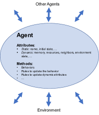
Figure 1: Each agent can interact with the environment or other neighbors in its neighborhood. Agents also have a set of static and dynamic attributes storing the properties of the agent and its knowledge about the surrounding agents and the environment. The simple rules that an agent is following are encoded in the methods.

Agents are completely autonomous entities in their decision making. As shown in Figure 1, every agent has a set of attributes and methods that define how and with whom it can interact. This defines the topology of an ABM system. Not all the agents are connected with each other; instead an agent is connected with a particular set of agents, called neighbors, who influence its localized decision making.

Definition 2 (Environment).

A set of entities that influence the behavior of an agent constitute the environment for an agent.

Figure 1 shows that agents interact not only with other agents but also with the environment.

To model a problem using ABM, we have to define the agents, the environment as well as associated methods and interactions in a way that reflects the original problem. It should be noted that the goal of our ABM approach is not to optimize the system, but to model the system as accurately as possible. The goal is to model the distributed optimization mechanisms that would converge reasonably to optimized solution by modeling the interactions of a decentralized system such that the complexity remains manageable.

II-B Road Traffic ABM Model

In order to explain the model (i.e., the agents and the environment of the ABM model), we start with the single intersection of roads. The visualization of this model is shown in Figure 2. The environment of our model is represented by the road. The agents in our model are:

• sensors

• traffic lights

• vehicles

• Decision Maker (DM)

This single intersection model contains 20 sensors. The sensors are represented by the black dots surrounding the perimeter of the roads. There are four traffic lights. These can be seen as the red/green dots near the center of the image. The yellow squares in Figure 2 symbolize vehicles traveling on the road. The blue square in the upper right section of the image represents a central DM that will be responsible for managing the timing of the traffic lights in the model.

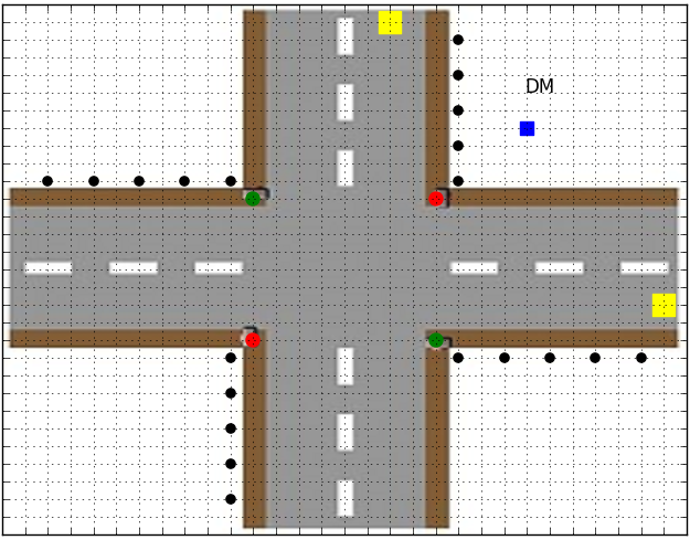
Figure 2: The sensors are represented by the black dots surrounding the perimeter of the road. The green and red dots are traffic lights. The vehicles are represented by yellow squares, and the DM is represented by a blue square in the upper right section.

The interaction between the sensor agents and the environment (the road) is modeled by the collection of traffic measurements. Those measurements represent the number of vehicles approaching the intersection. Once a sensor observes a vehicle approaching the intersection it tries to transmit this information to the DM.

The DM controls the timing of the four traffic lights with the aim of optimizing the waiting time of the vehicles traveling through the intersection. It is important to notice that we do not focus on the optimization algorithms related to the vehicle traveling time, we rather focus on the analysis of the communication aspects of the sensor network that collects the information about the traffic. In Figure 2, the traffic lights appear red and green in colour. The red colour symbolises that traffic should stop when it reaches the traffic light. The green colour represents that the vehicles are free to move past the traffic light.

Algorithm 1 Model

$T_{c}\leftarrow\textit{Current Tick number}$

$T_{max}\leftarrow\textit{Tick number limit}$

repeat

     Set tick_number to 0

     for each existing vehicle do

         if no car in front and green light then

              Move forward               

     if random_number $<$ probability of new vehicle then

         Create new vehicle      

     while $T_{c}<T_{max}$ or Transmission not succ. do

         Sensor attempt to transmit

         Increment $T_{c}$      

     if $T_{c}==T_{max}$ then

         DM make decision      

The model description is outlined with the Algorithm 1. The tick number limit ($T_{max}$) is a user defined parameter, that allows us to define the upper time limit for the sensor transmission attempts and at the same time the decision making interval of the DM agent. One tick is equivalent to a transmission time slot on the MAC layer. Since we dedicate one tick to the movement and generation of the vehicles and one additional tick for the DM decision making function, the number of ticks that is dedicated for the transmission of the measurements ($T_{trans}$) is calculated as:

$$T_{trans}=T_{max}-2$$ (1)

As shown in Algorithm 1, each car that is currently on the grid will attempt to move one space forward in each simulation iteration (one iteration takes $T_{max}$ ticks). For simplicity sake, the vehicles will always travel in a straight line. If there is already another vehicle in the space a certain car intends to move to or the space in front of that, it will not be allowed to move forward. This prevents vehicles from colliding with each other or travelling too close to each other. Vehicles are also prohibited from moving if they are close to a traffic light in their trajectory and the traffic light is red.

Each simulation iteration involves the creation of new vehicles on the grid. The number of vehicles added to the grid depends on the user defined parameter (prob. of new vehicle). Vehicles will only be initialized on the edges of the grid either traveling north, south, east or west. The initial position of the newly generated vehicles is chosen randomly (i.e., uniformly sampled from a list of all available positions). If there is already a vehicle currently blocking the placement of the newly generated vehicle, the newly generated vehicle will be discarded. Once the vehicles are placed on the grid and the existing vehicles move according to the above mentioned rules, the sensors collect the vehicle position information and attempt to convey those measurements to the DM. The sensors detect stopped vehicles by remembering the grid space where vehicles were detected in the previous cycle. If this grid space is still occupied by the same vehicle in the current cycle, that means that the vehicle has stopped moving. On the other hand, if the grid space is no longer occupied, the vehicle has moved on. We model the MAC layer protocols (i.e., TDMA, slotted Aloha and CSMA/CA) for the communication between the sensors and the DMs, and in the case of multiple intersections we also model the communication between the DMs (TDMA like scheduling). It is important to keep in mind that the implemented model is discrete (the time is divided into slots of equal duration). Each sensor can only transmit at the beginning of a slot. The chosen MAC protocol defines how to deal with potential collisions. A collision happens in case a sensor attempts to transmit in the same slot as one of its neighbors. A neighboring sensor is the one that is in the selected sensor’s Moore neighborhood. The Moore neighborhood represents the 8 grid spaces surrounding the selected sensor’s grid space. Hence, a sensor transmission is affected by the transmission of sensors in all directions, including diagonals.

In our analysis we consider three MAC protocols for the communication between the sensor nodes and the DMs, i.e., slotted Aloha, TDMA and CSMA/CA. Slotted Aloha deals with collisions by introducing back-off time, meaning that in case two neighboring sensors try to transmit at the same time, both transmissions will be unsuccessful and the sensors will choose a random back-off time to retry the transmission. The Aloha protocol also introduces a timeout time, which in case it is reached without a successful transmission implies that the packet should be discarded. As opposed to the Aloha protocol which does not involve any type of synchronization between the nodes and therefore, potentially leads to packet collisions, the TDMA protocol is implemented by allowing the DM to assign each sensor a specific time slot for packet transmissions. The centralized coordination, results in a collision free environment, if only one DM exists (i.e., the single intersection of roads scenario). In case multiple DMs are managing the communication of their sensors (i.e., Figure 4), we have to introduce some type of coordination between the DMs to avoid potential packet collisions. The CSMA/CA protocol, like Aloha, is an opportunistic approach. If a sensor has information to send, it first checks if any of its neighbours is currently using the spectrum resource. If the resource is currently being used, a back-off time will be computed. If the resource is not being used, the packet will be transmitted collision free and the DM will send an acknowledgment packet back to the sensor node to confirm the reception of the packet. It should be noted that the model assumes that there are no hidden nodes. Therefore, all potential collisions will be successfully sensed before transmission.

Figure 3: Traffic Light Finite State Machine describes the transition of the traffic lights between the three predefined states.

As shown in Algorithm 1, the final time slot of each cycle is reserved for the DM entity to make a decision. The DM analyzes the information received from the sensors and based on that controls the timing of the traffic lights. The traffic lights follow a strict set of rules, that can be summarized with the finite state machine shown in Figure 3. The traffic lights can be configured to be in one of three different states - State 0, State 1 and State 2. Figure 2 shows the system in State 1, allowing cars traveling eastwards and westwards to pass. In State 0, all traffic lights are red, and hence no vehicles are allowed to pass through any traffic lights. State 2 allows only vehicles traveling northbound or southbound to pass. The DM determines how long the traffic lights stay in a certain state, i.e., the DM based on the collected sensor information calculates the values of $T_{1}$ and $T_{2}$ in Figure 3. Figure 3 also shows that between each transition of State 1 and State 2, a period of 9 cycles in State 0 takes place. This period allows all traffic that has recently passed through the traffic lights to safely clear the intersection, preventing collisions with vehicles coming from other directions.

As previously mentioned, if we consider a more complex scenario (i.e., the four neighboring intersections scenario), we have to introduce coordination between the DMs. Again, our focus is not the coordination of the decision making functionalities of the DMs in order to optimize the traffic flow. Therefore, the states of the traffic lights are completely independent from each other. We focus on the optimization of the communication aspects of this scenario, meaning that the DMs coordinate the transmission time slots for their sensors in order to minimize the number of collisions. As shown in Figure 4, each intersection has 20 sensors, 4 traffic lights and one DM. The vehicles can now be generated in more locations compared to the basic model (i.e., one intersection model). We also define a neighbor radius set, that defines the distance between two sensors within which their transmissions could result in collisions.

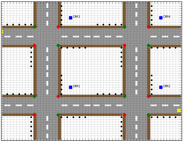
Figure 4: A four intersections model, showing all the sensors (black), traffic lights (red and green), vehicles (yellow) and decision makers (blue) that are part of our model.

In order to coordinate the transmissions for neighboring intersections we introduce a higher MAC layer, that schedules DMs in a TDMA like manner. Each DM gets its own dedicated time slot for the communication with its own sensors. We also introduce a relation between the higher and lower MAC layer time slot lengths. One slot on the higher MAC layer is the equivalent of 20 slots on the lower MAC layer. The lower MAC layer protocols are described previously (i.e., slotted Aloha, TDMA and CSMA/CA), whereas the higher MAC layer uses one of the following three approaches to coordinate the communication amongst multiple DMs: (1) Centralized Decision Maker, (2) Decentralized L-MAC and (3) DESYNC.

II-C Centralized Decision Maker

The approach that involves a Centralised Decision Maker (CDM) entity assumes that this centralized node has all the information needed to control all involved DMs. The centralized node needs to know how many time slots should be assigned to each DM and how to synchronize the activation of all DMs. As mentioned previously, our approach schedules 20 time slots, using a selected protocol - either TDMA, slotted Aloha or CSMA/CA, per DM in a round robin fashion.

II-D Decentralized L-MAC

This approach allows us to coordinate the transmission among multiple DMs by implementing a decentralized TDMA schedule by using the L-MAC protocol outlined in [24]. Each DM defines a probability vector of length $C$ where $C$ is the available number of time slots in a round. Initially, each DM chooses a transmission slot with equal probability. Based on the success and failure rate of transmission for the chosen transmission slot, the probability vector for each DM gets updated to allow a more intelligent choice of slots in the next round. The result of this is a collision-free schedule, provided that the number of DMs is less than $C$.

II-E DESYNC

The Desync algorithm is described in [25]. Each DM initializes a slot for the communication with its sensor nodes. Each DM also listens for messages that are transmitted by other DMs and stores the timestamps of transmissions that occurred before and after its own slot. This information is used by the DMs to adjust their own slot, by computing the midpoint between the previous and next slot. The method described in [25] is concerned with a continuous model. We had to adapt this in order to fit our discrete model. The midpoint ($T_{m}$) between the previous ($T_{p}$) and next ($T_{n}$) time slot is computed as,

$$T_{m}=\Bigl{\lfloor}{\frac{T_{p}+T_{n}}{2}}\Bigr{\rfloor}$$ (2)

Equation (2) was further adapted to deal with the periodic nature of our timestamps (i.e., time cycles). For example, let us assume that the round time is $T_{r}=10$, $T_{p}=8$, and $T_{n}=2$. The midpoint slot ($T_{m}$) calculated for the next round should be equal to 10. However, using equation (2) it results in $T_{m}=5$. Therefore, if $T_{p}$ or $T_{n}$ is greater than the current firing slot number, the following equation should be used:

$$T_{m}=\Bigl{\lfloor}{\frac{T_{p}+T_{n}+T_{r}}{2}}\Bigr{\rfloor}$$ (3)

This ensures that each DM will position itself in the midpoint slot between the DMs transmitting before and after it, resulting in a collision free TDMA schedule.

III Simulation Study

The model was built using the ABM Python library Mesa [26]. Mesa is an open source framework that is built with the functionality of popular ABM simulation software such as NetLogo, Repast and Mason. Mesa’s DataCollector module allows us to easily collect data from the agents in the model at specified intervals. Mesa enables us to visualize the entire system at each simulation step, helping with the debugging and verification of the traffic lights finite state machine.

In this section, we present the simulation results for both scenarios: (1) uncoordinated and (2) coordinated. The results are generated for a varying range of input parameters, such as selection of MAC protocols, number of time slots available for the DMs on the higher MAC layer and neighbor radius. The results are evaluated using the accuracy of information and the spectrum utilization as criteria.

The accuracy of the information received by the DMs is important to the overall functionality of the system. The actual number of vehicles waiting at a given moment at the traffic lights is denoted by $N_{W}$. The number of vehicles that has been registered by the sensor nodes is denoted by $N_{S}$, and the number of vehicles that has been reported to the DM is $N_{DM}$. Since we focus on the communication aspects of the system, we assume perfect sensing implying $N_{S}=N_{W}$. We define accuracy of information as,

$$A=N_{DM}-N_{S},$$ (4)

which implies that the accuracy of information is the difference between the number of vehicles reported to the DM and the actual number of vehicles waiting at the traffic lights. A positive error ($A>0$) means that the DM believes that there are more vehicles waiting than the actual figure. A negative error ($A<0$) means that the DM believes that there are less vehicles waiting than the actual ones. This data is collected once every cycle before the DM action step outlined in Algorithm 1. Since we assume perfect sensing ($N_{S}=N_{W}$), any discrepancies can be attributed to interference within the system, i.e., collisions of packets transmitted from neighboring nodes in the same tick.

The spectrum utilization is a metric that allows us to understand what proportion of the available information in the system is actually transferred to the DM in order to make a more informed decision about the traffic light states. For example, if there are 5 vehicles waiting, the total amount of information/packets that should be available at the DM is 5. If 2 sensors successfully utilize the spectrum, the utilization is 40%. Therefore, if the number of successfully transmitted packets in a cycle is denoted with $N_{succ}$ and the actual number of vehicles waiting at the traffic lights is $N_{W}$, the spectrum utilization is calculated as:

$$U=\frac{N_{succ}}{N_{W}}$$ (5)

III-A Uncoordinated Scenario

The uncoordinated scenario assumes that the DMs are not aware of each other’s scheduling decision, meaning that increasing the number of neighboring intersections will lead to an increase in the number of collisions, due to the lack of coordination between the neighboring DMs.

Figure 5 shows the average value of the accuracy of information gathered over $10^{4}$ simulation steps for the single intersection of roads scenario. The neighbor radius is set to 15, meaning that sensors that are within 15 hops away can potentially interfere with each other.

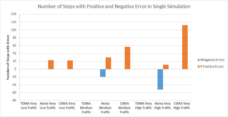
Figure 5: Accuracy of Information for the single intersection of roads scenario. The neighbor radius is set to 15.

Figure 5 highlights that the choice of protocol and level of traffic affect the accuracy of information received by the DM. Regardless of traffic level, the model using the TDMA protocol make transmissions with zero error, resulting in highly accurate results. In a single intersection model, each sensor is allocated its own time slot to send. Therefore, there are no collisions of packets in a slot, resulting in highly accurate data transmission to the DM. Thus, the DM is always aware of exactly how many vehicles are currently waiting.

When there is low traffic, the model using the slotted Aloha protocol is seen to have a number of positive errors. The positive errors are due to backed off sensor packets being transmitted when they no longer reflect the state of the system (i.e., a collision happens, all involved sensors decide to retransmit the packets and in the meantime, the traffic lights change state and the number of vehicles waiting changes). The DM is not aware that the received information is stale and therefore continues to control the timing based on inaccurate information. The accuracy of information for the slotted Aloha protocol changes as the number of vehicles waiting grows. This is due to the fact that with the increasing number of waiting vehicles the number of sensors trying to transmit their measurements increases. The increased number of transmissions results in an increasing number of collisions, leading to the case in which the DM does not have the information about a significant number of vehicles waiting on the lights ($N_{DM}<<N_{S}$).

The model using the CSMA/CA protocol does not suffer from any negative errors. As expected the number of positive errors increases with the increasing level of traffic. The reason for this stems from the increased number of sensors attempting to transmit packets when there is a higher traffic level. When the traffic lights change state, there is a sudden reduction in the amount of packets competing for spectrum access as the vehicles begin to move. This leads to an increased amount of packets reaching the DM with inaccurate information ($N_{DM}>>N_{S}$).

As previously mentioned, we also calculate the spectrum utilization as shown in equation (5). The results in Figure 6 are obtained over $10^{4}$ simulation steps on a two intersection model. Considering the uncoordinated nature of the scenario (2 DMs that are not aware of each others scheduling decisions) 40 ticks are assigned for the sensors to transmit the vehicle detection information per cycle. We up-scaled the model (from one to two intersections) in order to increase the range of neighboring radii. We vary the neighbor radius from 5 to 25. All the scenarios assume an intermediate traffic level, i.e., a 0.5 probability of a car being generated each cycle.

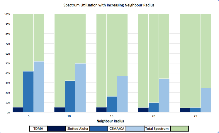
Figure 6: Spectrum Utilization - showing how much of the available information in the system is actually transferred to the DM in order to make a more informed decision about traffic light system.

Figure 6, as expected, shows that TDMA exhibits the lowest spectrum utilization. However, it is not affected as much by neighbour radius. When the neighbour radius is large, there is a low probability that two sensors from different intersections within the same neighbour radius would be scheduled for the same tick, both having vehicles waiting at them. Hence, the spectrum utilisation for the TDMA protocol remains fairly constant regardless of the neighbor radii. CSMA/CA displays the greatest spectrum utilisation in all variations of neighbor radii. This is due to the sensing first - transmitting if available policy of the CSMA/CA protocol. This allows sensors to avoid collisions of packets by sensing the collision before it occurs and backing off for a random period of time. In comparison to this, slotted Aloha demonstrates a relatively high spectrum utilization when the neighbor radius is low. The increase of the neighbor radius leads to the increasing number of collisions (due to lack of coordination and sensing), which results in lower spectrum utilization.

III-B Coordinated Scenario

The coordinated scenario assumes that the DMs are aware of each other’s scheduling. As previously explained, in order to coordinate the scheduling mechanisms of the DMs, we introduce a higher MAC layer. The coordination is achieved by either a Centralised Decision Maker, Desync or the L-MAC protocol. The operation of the Centralised Decision Maker is obvious - manually configured time slots for each DM. Therefore, we are going to explain in more detail how the Desync and L-MAC protocols achieve the best time slot assignment on the higher MAC layer.

III-B1 Desync Algorithm

Desync algorithm relies on the fact that each node in the system performs a task periodically. Depending on the length of the cycle, the convergence of the system can display different behavior. Figure 7(a) depicts a simple scenario in which four DMs coordinate their communication periods. The ring represents the value of $T$, the total time taken for a full round to be completed. A colored circle with a number in the middle represents the DM, that assigned a time slot. An empty circle represents a slot where no DM is assigned and therefore remains idle. A round time of four is chosen for this simulation. Each node is given a unique starting point. The system executes the Desync algorithm. However, since the nodes are already maximally spaced apart, no further movement takes place.

(a)

(b)

Figure 7: Desync (a) T=4 (b) T=8

A round time of 8 is chosen in the next example. Figure 7(b) shows that all the nodes representing the DMs start close to each other in a round. The Desync algorithm allows the nodes to rearrange themselves around the ring so that they are maximally spaced apart, and that is when the system converges (last image in Figure 7(b)).

The next example is configured with a round time of 6 (Figure 8). Theoretically, there is no possible configuration to ensure maximal spacing between the DM time slots. Therefore, the system never converges. Figure 8 shows that the nodes continue to rearrange themselves in such a way that a circular pattern emerges. The nodes rotate counter-clockwise around the ring. This implies that a round time should be chosen such that the number of DMs is a factor of the round time.

Figure 8: Desync T=6

III-B2 L-MAC Protocol

The method used by the L-MAC protocol to implement a TDMA schedule is quite different from the Desync protocol. Initially, the DMs choose a random slot in the schedule with equal probability. This is in contrast to the Desync protocol where nodes are assigned a starting point. If there is a collision in a slot, the DM will choose a slot again in the next round with updated probabilities. If the DM is successful in a slot, it will choose the same slot again in the next round with a higher probability.

Figure 9(a) shows the convergence of the system to a collision free configuration. Each node that experiences collisions continues to rearrange itself, until a collision free schedule is reached. In Figure 9(a), if we take a closer look at DM3, we see that due to a collision free assignment in a previous slot, the node decides to stick with the chosen slot even after it experiences collisions.

(a)

(b)

Figure 9: L-MAC (a) C=4 (b) C=6

As proven in [24], the system can converge with any round time that is greater than the number of available DMs. For the sake of comparison with the Desync protocol, in Figure 9(b), we show that the L-MAC protocol can converge with a round time of 6. However, the L-MAC protocol does not consider the spacing of the nodes around the ring.

Increasing the round time leads to an increasing number of idle slots, which implies that the probability of a node initially choosing slots without collisions increases as well. That results in a shorter convergence time. Though very unlikely, it is still possible that the DMs randomly choose a collision free schedule on initial selection with any number of slots in a round greater or equal to the number of DMs.

Similar to the approach adopted to analyze the uncoordinated scenario, we will focus on the analysis of the accuracy of information and the spectrum utilization for the coordinated scenario. The coordinated scenario can be implemented by using any of the abovementioned high layer MAC protocols. The number of time slots available on the higher MAC layer is set to four, meaning that all mentioned higher level MAC protocols would converge to the same arrangement. We used L-MAC in our simulations. The higher-lower MAC level time slot length has the ratio of 1:20, meaning that for every higher level MAC time slot allocated to a DM, the equivalent of 20 lower MAC ticks for sensor transmissions is available. Figure 10 shows the absolute error (absolute value of the accuracy of information). The data used in Figure 10 is obtained from simulations of the four intersections model. The traffic level is set to medium, i.e., a vehicle will be generated with the probability 0.5 in each cycle. The neighbor radius is set to 10. Figure 10 depicts the average spread of the absolute error observed over 10 simulations with 5000 simulation steps each. The absolute error is used in this case as it is not our intention to imply a median error close to zero. The TDMA results are not shown in Figure 10, because TDMA results in an average spread of zero for both uncoordinated and coordinated scenarios. The data in Figure 10 is shown in the form of a box plot. The upper extreme of the error bars show the average maximum absolute error, the lower extreme of the error bar shows the minimum average absolute error. The upper lines of the boxes in the graph represent the upper quartiles, the lower lines represents the lower quartiles. The lines in the centers of each box represents the median values of the absolute error.

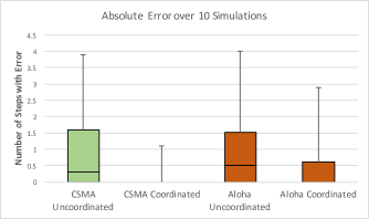
Figure 10: Absolute Error - the data is obtained from simulations of the four intersection model; traffic level is set to medium; the neighbor radius is set to 10.

Figure 10 shows that the introduction of the higher MAC layer can greatly reduce the average absolute error for both CSMA/CA and slotted Aloha. The introduction of coordination reduced the average maximum absolute error from 3.9 to 1.1 for CSMA/CA and from 4 to 2.6 for slotted Aloha. The average median absolute error was also reduced from 0.3 to 0 for CSMA/CA and from 0.5 to 0 for slotted Aloha. The reason for the reduction in the absolute error lies in the influence of the higher MAC layer scheduling procedures. Sensors can only transmit data to the target DM when the target DM is selected by the higher MAC layer. This decreases the problem of stale data. Since the ABM approach allows us to analyze each time step of the discrete simulation, the analysis of the log files shows that the majority of stale data is received immediately after a car moving step, mostly affecting the earliest ticks in each cycle. When a higher MAC layer is introduced, stale data primarily affects the first DM that is selected after a movement step. Previously, all four DMs would be affected by this stale information. The stale information will indeed only affect the sensors’ packets that are being sent to the first DM selected after a movement step, as the selected DM will reject all other sensor packets being transmitted to other DMs. Because each DM is allocated its own slot, the interference from sensors transmitting to other DMs is decreased, and thus the accuracy of information received by the DMs is improved.

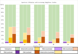
Figure 11: Spectrum Utilization - comparison between the coordinated and uncoordinated scenario, showing how much of the available information in the system is actually transferred to the DM.

Figure 11 shows the comparison between the spectrum utilization for the coordinated and uncoordinated scenario. The results are gathered from the simulations of the two intersection model over $10^{4}$ simulation steps. The traffic level is again configured to be medium. This is the same configuration that was used to obtain the spectrum utilization of the uncoordinated model shown in Figure 6. The L-MAC protocol is used with a round time of two, and a higher to lower ratio of 1:20. Therefore, after convergence these should be no idle slots in the higher MAC layer. This choice of parameters ensures fairness between the uncoordinated and coordinated scenarios. Two higher MAC layer ticks in the coordinated scenario with the ratio of 1:20 results in a total of 40 time slots for the communication between the sensors and the DMs. In the uncoordinated scenario, 40 time slots are assigned for sensor transmissions in each cycle.

The results obtained from these simulations are overlaid with the results obtained from the uncoordinated model as shown in Figure 11. It should be noted that Figure 11 is not a stacked bar chart, meaning that the ratio between each scenario and the total spectrum is being analyzed. As shown in Figure 11, the spectrum utilisation is reduced when coordination is introduced. This is due to the limitation that only sensors transmitting to the selected DM are able to send in each slot. The neighbor radius has a similar effect on the slotted ALOHA and CSMA/CA protocols in the uncoordinated and coordinated scenarios (i.e., the spectrum utilization decreases with increasing neighbor radius). Again TDMA is not affected by the neighbor radius. As previously explained, in the coordinated TDMA scenario, each DM is assigned its own higher MAC TDMA slot to transmit where each sensor will then be given its own lower level MAC tick to transmit. The spectrum utilization of TDMA in the coordinated scenario is approximately half the spectrum utilization achieved in the uncoordinated scenario. This is due to the rejection of packets attempting to transmit to DMs that are not selected by the higher MAC layer.

IV Discussion and Conclusion

The increasing complexity of the next generation of communication networks leads to a need to change the tools we use to model and analyze them. The primary purpose of our work is to investigate the possibility of using ABM as a method of modeling an IoT network. We show that ABM is an effective way to model the complex behavior of heterogeneous nodes (e.g., simple sensors, traffic lights, and more powerful decision making nodes). One of the main advantages of ABM is its flexibility in modeling networks that does not scale up exponentially with the size (e.g., from the simple one intersection model, to the more complex two and four intersections model). Besides, it provides opportunity to add new features for decision coordination (e.g., the higher MAC layer protocol to ensure coordination between the decision makers). Human interactions (e.g. vehicles) are as easily configurable as the network agents in the model (e.g. sensors). This feature allowed the level of traffic and behavior of the vehicles to be modeled as well as the operation of the network. Another appealing quality of the ABM modeling approach is its ability to model and collect information on a more granular level (i.e., from all agents within the system in any time step of the simulation).

In the models where CSMA/CA is used as the selected MAC protocol, we assume there are no hidden nodes. If hidden nodes were introduced, the behavior and performance of the models using the CSMA/CA protocol could change. Moreover, we assumed that the only interference in the model is generated from the agents within the IoT network itself. Although the results in Section III suggest TDMA to be an extremely effective MAC protocol, the limitations of our present model do not highlight the areas where TDMA can fail. For example, if a sensor fails to transmit successfully due to external source of interference, it has to wait for its slot in the next cycle to transmit. As explained in Section II, the DM uses a method of polling for a certain amount of time before making timing decisions. If this was more of a continuous decision making process, TDMA could be found to be slower than the other protocols as each sensor must wait for its time slot and for the polling phase to be over, before transmitting. Therefore, more investigations are necessary before concluding in a definite way that TDMA is the best MAC protocol for the kind of application considered in this paper and a subject of future research.

The motivation for this paper is to investigate ABM as a tool for modeling the complexity of future networks. Building on this work, we envision the future research to be about modeling of complex networks where ABM can help to reduce overhead and complexity of distributed decision making.

ABM

Agent-Based Modeling

5G

Fifth Generation

IoT

Internet of Things

MAC

Medium Access Control

CCS

Complex Communication Science

WSN

Wireless Sensor Network

DM

Decision Maker

CDM

Centralised Decision Maker

References

- [1] J. Grady, System Synthesis: Product and Process Design. CRC Press, 2010.
- [2] I. Macaluso, H. Cornean, N. Marchetti, and L. Doyle, “Complex communication systems achieving interference-free frequency allocation,” in Communications (ICC), 2014 IEEE International Conference on, June 2014, pp. 1447–1452.
- [3] I. Macaluso, C. Galiotto, N. Marchetti, and L. Doyle, “A Complex Systems Science Perspective on Wireless Networks,” Journal of Systems Science and Complexity, no. 10, pp. 1–27, 2016.
- [4] C. M. Macal and M. J. North, “Tutorial on agent-based modeling and simulation,” in Proceedings of Conference on Winter Simulation, ser. WSC ’05. Winter Simulation Conference, 2005, pp. 2–15.
- [5] ——, “Tutorial on agent-based modeling and simulation part 2: How to model with agents,” in Proceedings of the 2006 Winter Simulation Conference, Dec 2006, pp. 73–83.
- [6] U. Wilensky and W. Rand, An introduction to agent-based modeling: modeling natural, social, and engineered complex systems with NetLogo. MIT Press, 2015.
- [7] M. Pogson, R. Smallwood, E. Qwarnstrom, and M. Holcombe, “Formal agent-based modelling of intracellular chemical interactions,” Biosystems, vol. 85, no. 1, pp. 37 – 45, 2006.
- [8] I. Benenson, K. Martens, and S. Birfir, “Parkagent: An agent-based model of parking in the city,” Computers, Environment and Urban Systems, vol. 32, no. 6, pp. 431 – 439, 2008, geoComputation: Modeling with spatial agents.
- [9] S. Laghari and M. A. Niazi, “Modeling the internet of things, self-organizing and other complex adaptive communication networks: a cognitive agent-based computing approach,” PloS one, vol. 11, no. 1, 2016.
- [10] P. Twomey and R. Cadman, “Agent-based modelling of customer behaviour in the telecoms and media markets,” Digital Policy, Regulation and Governance, vol. 4, no. 1, pp. 56–63, 2002.
- [11] C. Douglas, H. Lee, and W. Lee, “A computational agent-based modeling approach for competitive wireless service market,” Piscataway, NJ, USA, 2011, p. 6 pp.
- [12] A. Tonmukayakul and M. B. Weiss, “An agent-based model for secondary use of radio spectrum,” New Frontiers in Dynamic Spectrum Access Networks (DySPAN), 2005.
- [13] D. Horváth, V. Gazda, and J. Gazda, “Agent-based modeling of the cooperative spectrum management with insurance in cognitive radio networks,” EURASIP Journal on Wireless Communications and Networking, vol. 2013, no. 1, p. 261, 2013.
- [14] M. Niazi and A. Hussain, “Agent-based tools for modeling and simulation of self-organization in peer-to-peer, ad hoc, and other complex networks,” Communications Magazine, IEEE, vol. 47, no. 3, pp. 166–173, 2009.
- [15] M. Liu, Y. Xu, and A.-W. Mohammed, “Decentralized opportunistic spectrum resources access model and algorithm toward cooperative ad-hoc networks,” PloS one, vol. 11, no. 1, 2016.
- [16] M. A. Niazi and A. Hussain, “A novel agent-based simulation framework for sensing in complex adaptive environments,” IEEE Sensors Journal, vol. 11, no. 2, pp. 404–412, 2011.
- [17] S. Coleri, S. Y. Cheung, and P. Varaiya, “Sensor networks for monitoring traffic,” in Allerton conference on communication, control and computing, 2004, pp. 32–40.
- [18] M. Tubaishat, Y. Shang, and H. Shi, “Adaptive traffic light control with wireless sensor networks,” in Proceedings of IEEE consumer communications and networking conference, 2007, pp. 187–191.
- [19] S. Y. Cheung, S. C. Ergen, and P. Varaiya, “Traffic surveillance with wireless magnetic sensors,” in Proceedings of the 12th ITS world congress, vol. 1917, 2005, pp. 173–181.
- [20] J. Ma, B. L. Smith, and X. Zhou, “Personalized real-time traffic information provision: Agent-based optimization model and solution framework,” Transportation Research Part C: Emerging Technologies, vol. 64, pp. 164 – 182, 2016.
- [21] K. Hager, J. Rauh, and W. Rid, “Agent-based modeling of traffic behavior in growing metropolitan areas,” Transportation Research Procedia, vol. 10, pp. 306 – 315, 2015.
- [22] A. Lansdowne, Traffic simulation using agent-based modelling. University of the West of England, 2006.
- [23] N. J. Kaminski, M. Murphy, and N. Marchetti, “Agent-based modeling of an iot network,” in IEEE International Symposium on Systems Engineering (ISSE), Oct 2016, pp. 1–7.
- [24] M. Fang, D. Malone, K. R. Duffy, and D. J. Leith, “Decentralised learning MACs for collision-free access in WLANs,” Wireless networks, vol. 19, no. 1, pp. 83–98, 2013.
- [25] J. Degesys, I. Rose, A. Patel, and R. Nagpal, “DESYNC: self-organizing desynchronization and tdma on wireless sensor networks,” Proceedings of international conference on Information processing in sensor networks, pp. 11–20, 2007.
- [26] D. Masad and J. Kazil, “Mesa: An agent-based modeling framework,” 14th PYTHON in Science Conference, 2015.