Memoirs of a giant planet

Abstract

Saturn is ringing, weakly. Exquisite data from the Cassini mission reveal the presence of f-mode oscillations as they excite density waves in Saturn’s rings. These oscillations have displacement amplitudes of order a metre on Saturn’s surface. We propose that they result from large impacts in the past. Experiencing little dissipation inside Saturn on account of its weak luminosity, f-modes may live virtually forever; but the very ring waves that reveal their existence also remove energy from them, in $10^{4}$ to $10^{7}$ yrs for the observed f-modes (spherical degree $2-10$). We find that the largest impacts that arrive during these times excite the modes to their current levels, with the exception of the few lowest degree modes. To explain the latter, either a fortuitously large impact in the recent past, or a new source of stochastic excitation, is needed. We extend this scenario to Jupiter which has no substantial rings. With an exceedingly long memory of past bombardments, Jovian f-modes and p-modes can acquire much higher amplitudes, possibly explaining past reports of radial-velocity detections, and detectable by the Juno spacecraft.

1. Introduction

Seismology has long been a valuable probe of the interiors of the Earth and Sun. But for giant planets, oscillations have not been detected until recently. Stevenson (1982) first proposed that the rings of Saturn can act like a giant seismograph. An oscillating mode within Saturn produces density perturbations. These produce an oscillating gravitational field which can launch a density wave in Saturn’s rings, at the location of the mode’s Lindblad resonance. Marley (1991) and Marley & Porco (1993) refined Stevenson’s proposal, showing that Saturn’s prograde, sectoral (i.e., with spherical harmonic integers $l=m$) f-modes will produce detectable features in Saturn’s C-rings, provided surface displacements are over about 1 metre. These, Marley & Porco (1993) argued, could explain some of the features seen in the Voyager data that are un-associated with any known satellites. They also showed that f-modes with $l-m=1$ can produce vertical bending waves in the rings, and those with larger values of $l-m$ can also perturb the rings, albeit with smaller amplitude.

Such a scenario has been unambiguously confirmed recently. By careful analysis of the Cassini stellar occultation data, Hedman & Nicholson (2013, 2014); Hedman et al. (2018); French et al. (2019) identified density waves associated with all of the prograde, sectoral f-modes with $\ell\leq 10$. The association of an observed density wave with an internal mode is made by observing both the number of spiral arms and the pattern frequency of the wave, and then comparing with theoretical f-mode frequencies. Frequencies calculated by Mankovich et al. (2018) show excellent agreement with those inferred from the observed pattern frequencies (also see previous works by Vorontsov et al., 1976; Vorontsov & Zharkov, 1981). In addition to density waves launched by sectoral f-modes, a number of other ring waves have also been observed, including density waves due to f-modes with $l-m=2$ and 4, and bending waves due to f-modes with $l-m=1$, 3, and 5 (Mankovich et al., 2018; French et al., 2019).

The detection of Saturn’s oscillations opens a new window into the internal properties of that planet. By comparing observed and theoretical f-mode frequencies, one can learn about Saturn’s background state. For example, Mankovich et al. (2018) inferred the bulk rotation rate with a precision of 10%. Fuller (2014) and Fuller et al. (2014) showed that one of the observational surprises— specifically, that the density waves associated with $m=2$ and $m=3$ prograde sectoral f-modes appear to be split into multiple waves with slightly different frequencies—can be explained by f-mode mixing with g-modes. This provides evidence for stable stratification near Saturn’s core.

In this work, we are concerned with a different issue. The observed ring waves have dimensionless amplitudes that range from a few percent to unity. These, when translated into f-mode amplitudes, imply surface displacements all within an order of magnitude of $1$ meter (see Table 1 below). This appears to be rather fortuitous: if the mode amplitudes were much less than a meter, the ring waves will be too weak to be visible. Why is Saturn oscillating at the amplitudes that we observe? And in tandem, what excites these oscillations in Saturn?

Oscillations in stars are known to be driven by linear instabilities (e.g., the $\kappa$-instability as for Cepheids and RR Lyraes), or stochastic processes (e.g., turbulent convection for the Sun and red giants). Saturn’s oscillations must belong to the latter category. Mode amplitudes are so small (dimensionless amplitudes $\sim 10^{-9}$) that their damping must be linear. Hence if their excitation was linear too, the mode amplitudes would grow (or shrink) indefinitely. Stochastic driving, on the other hand, can lead to a variety of outcomes. Consider the example of throwing pebbles at a bell. The pebbles come at random intervals and excite the bell’s oscillation incoherently. Given a long enough time, the bell will settle into the so-called fluctuation-dissipation equilibrium, with a ringing volume that depends on, among other things, how hard a pebble is thrown, how many pebbles are thrown per unit time, and how quickly the bell loses energy.

What stochastic process could be operating inside a giant planet? Much discussion in the past has focused on turbulent convection. Although Saturn is likely fully convective, we argue here that its internal flux is too low, and convection too feeble, to explain the observations. Instead, we propose that past impacts drive these modes to the observed amplitudes.

Stimulated by the comet Shoemaker-Levy 9’s impact onto Jupiter, Kanamori (1993); Marley (1994); Lognonne et al. (1994); Dombard & Boughn (1995) considered how impacts affect internal oscillations (also see Markham & Stevenson, 2018). But these studies only considered small bodies like SL9, which has a radius of $R\sim 2\,\rm km$. They failed to consider the role of an additional axis, that of time.

If the f-modes are very weakly damped, they can have a long memory of past impacts, including by bodies much larger than the SL9 comet. Here, we explore this direction by first studying how weakly damped the modes are (§3,4), finding that the ring waves, as opposed to internal dissipation in Saturn, dominate the damping. We then expose the failure of previously proposed mechanisms in exciting the f-modes to their observed amplitudes (§5), before turning to consider how past large impacts can contribute (§6). Having calculated in detail the case for Saturn, we extrapolate our calculations to Jupiter, and find that there are observable consequences (§7).

Much of the discussions in this work are order-of-magnitude in nature, as some physics is difficult to model in detail.

2. Preparation: f-modes in Saturn

We assemble some scalings for f-modes that are of use throughout this paper. The asymptotic expression for f-mode frequency as a function of spherical degree $\ell$ is

$$\omega^{2}={{GM_{s}}\over{R_{s}^{3}}}\sqrt{\ell(\ell+1)}\,,$$ (1)

where $M_{s},R_{s}$ are Saturn’s mass and radius, respectively. This expression coincides fairly well with results from eigenmode calculations, under the Cowling approximation (also see Mankovich et al., 2018, without Cowling). There is no $\ell=1$ f-mode – although the Cowling approximation (as we adopt here) may give it a non-zero frequency, this mode should have zero frequency in the full solution (Christensen-Dalsgaard & Gough, 2001).

We ignore the effects of planet rotation on the eigenfunction and split the eigenfunction into angular and radial dependencies as in eq. (A3). The displacement vector is $\xi$, and we define a normalized displacement vector ${\tilde{}\mbox{\boldmath$\xi$}}$ that satisfies

$$\int d^{3}r\rho{\tilde{}\mbox{\boldmath$\xi$}}\cdot{\tilde{}\mbox{\boldmath$\xi$}}=M_{s}R_{s}^{2}\,,$$ (2)

which implies that ${\tilde{\xi}}$ has the dimension of length. We focus on the radial dependency of the eigenfunction here. For f-modes, the surface radial displacement satisfies the following scaling,

$${\tilde{\xi}}_{r}(r=R_{s})\approx 1.8R_{s}\times\sqrt{\ell(\ell+1)}\,.$$ (3)

This rises with $\ell$ because high-$\ell$ f-modes are more concentrated towards the surface. The physical radial displacement is obtained by multiplying the above value by $Y_{\ell m}(\theta,\phi)$.

Energy stored in a f-mode (including gravitational, compressional and kinetic) is

$$E_{\rm mode}={1\over 2}\omega^{2}\int d^{3}r\rho\mbox{\boldmath$\xi$}\cdot\mbox{\boldmath$\xi$}\,.$$ (4)

With eqs. (1) and (3), this yields

$$E_{\rm mode} = {{\sqrt{\ell(\ell+1)}}\over 2}{{GM_{s}^{2}}\over{R_{s}}}\left({{\xi_{r}}\over{\tilde{\xi}_{r}}}\right)^{2}$$ (5)

$$\approx {{2\times 10^{26}}\over{\sqrt{\ell(\ell+1)}}}\,\rm erg\times\left({{\xi_{r}}\over{1\,\rm m}}\right)^{2}\,,$$

where $\xi_{r}$ is that evaluated at the planet surface.

Density perturbations by an f-mode produce perturbations in the gravitational potential. For a Eulerian density perturbation of the form $\rho^{\prime}(\mathbb{r})=\rho^{\prime}(r)Y_{lm}(\theta,\phi)$, the perturbed potential outside of Saturn is

$$\Phi_{lm}(\mathbb{r})=-4\pi{GM_{s}\over R_{s}}{1\over 2l+1}{R_{s}^{l+1}\over r^{l+1}}Y_{lm}(\theta,\phi)J_{lm}$$ (6)

where $J_{\ell m}$ is the gravitational moment (Binney & Tremaine, 2008; Marley & Porco, 1993) and

$$J_{\ell m} = {1\over{M_{s}R_{s}^{\ell}}}\int_{0}^{R_{s}}r^{\prime\ell}\rho^{\prime}(r^{\prime})Y_{\ell m}(\theta^{\prime},\phi^{\prime})Y_{\ell m}^{*}(\theta^{\prime},\phi^{\prime})\,d^{3}r^{\prime}$$ (7)

$$= {1\over{M_{s}R_{s}^{\ell}}}\int_{0}^{R_{s}}r^{\prime\ell}\rho^{\prime}(r^{\prime})r^{\prime 2}dr^{\prime}\,.$$

An orbiter, be that a particle in Saturn’s ring, or a man-made spacecraft orbiting the planet, can measure this potential variation. Numerically, this can be adequately approximated as

$$J_{\ell m}\sim 0.6\left({{\xi_{r}}\over{\tilde{\xi}_{r}}}\right)\sim{{5.8\times 10^{-9}}\over{\sqrt{\ell(\ell+1)}}}\left({{\xi_{r}}\over{1\,\rm m}}\right)\,.$$ (8)

for all $\ell$-values of practical interest.

3. F-modes are damped by the Rings

Saturn’s f-modes are visible thanks to its sensitive rings. In the following, we first show that Saturn’s rings is a leading player in removing energies from the normal oscillations, via the very density waves that reveal their presence. We then estimate the corresponding f-mode energies, based on the observed amplitudes of these density waves. Both of these results set stringent constraints on possible excitation mechanisms for the f-modes.

3.1. Damping time

We calculate the timescale on which density waves in the C-ring damp f-modes:

$$t_{\rm damp}\equiv{{E_{\rm mode}}\over{\dot{E}_{\rm wave}}}\,,$$ (9)

where $\dot{E}_{\rm wave}$ is energy input rate into density waves and $E_{\rm mode}$ is the mode energy in Saturn. The former is $\dot{E}_{\rm wave}=\omega_{p}\Gamma$, where $\omega_{p}$ is the angular pattern frequency of the wave (defined below) and $\Gamma$ is given by the standard torque formula (Goldreich & Tremaine, 1978):

$$\Gamma=-m\pi^{2}{\Sigma\over rdD/dr}\Psi_{lm}^{2}\,,$$ (10)

where

$$\Psi_{lm}\equiv{rd\Phi_{lm}\over dr}+{2\Omega\over\Omega-\omega_{p}}\Phi_{lm}\,.$$ (11)

Here, $\Sigma$ is the ring’s surface density, $\Omega=\Omega(r)$ is the Keplerian frequency at distance $r$, and all quantities are to be evaluated at the Lindblad resonance, i.e., where $D\equiv\Omega^{2}-m^{2}(\Omega-\omega_{p})^{2}=0$. For the special case of outer Lindblad resonances of sectoral modes ($|m|=l$), the potential (eq. 6) evaluated in the ring plane yields

$$|\Psi_{ll}| = (3l+1)|\Phi_{ll}|$$ (12)

$$= \left[4\pi{3l+1\over 2l+1}\left({2l+1\over 4\pi}{1\over(2l)!}\right)^{1/2}{(2l)!\over 2^{l}l!}{.84\over(l(l+1))^{1/4}}\right]$$

$$\times{GM_{s}\over R_{s}}{R_{s}^{l+1}\over r^{l+1}}\left({E_{\rm mode}\over GM_{s}^{2}/R_{s}}\right)^{1/2}$$

after using Equations (5) and (8) to relate $J_{ll}$ to $E_{\rm mode}$. Therefore,

$${1\over t_{\rm damp}} = {{\omega_{p}\Gamma}\over E_{\rm mode}}={1\over\omega_{p}}\pi^{2}{\Sigma(l+1)\over 3l}|\Psi_{ll}|^{2}{1\over E_{\rm mode}}$$ (13)

$$= {G\Sigma\over\omega_{p}R_{s}}\left({R_{s}^{l+1}\over r^{l+1}}\right)^{2}$$

$$\times\left[{0.7\cdot 4\pi^{3}(l+1)^{1/2}(3l+1)^{2}(2l)!\over 3l^{3/2}(2l+1)2^{2l}(l!)^{2}}\right]\,.$$

Table 1F-mode properties, as inferred from ring seismology

$l=|m|$	$\omega_{p}$	$r_{\rm Lindblad}$	$t_{\rm damp}$	$\Sigma$	$t_{\rm damp}$	$\Delta\Sigma/\Sigma$	$E_{\rm mode}$	$\xi_{r}$
units:	$[10^{-4}$s${}^{-1}]$	$[R_{s}]$	$[\Sigma_{1}^{-1}$Myr]	$[\,\rm g/\,\rm cm^{2}]$	[Myr]		$[10^{25}$ erg]	$[\,\rm m]$
2	3.76	1.45	0.15	4.0	0.037	0.47	0.28	0.18
3	3.50	1.41	0.30	6.9	0.044	0.56	2.15	0.61
4	3.35	1.39	0.25	5.8	0.10	0.39	1.38	0.56
5	3.22	1.39	1.27	5	0.25	0.12	0.21	0.24
6	3.11	1.40	2.83	5	0.57	0.056	0.10	0.18
7	3.01	1.41	6.52	5	1.3	0.082	0.52	0.44
8	2.94	1.42	15.4	5	3.1	0.050	0.47	0.45
9	2.87	1.43	37.0	5	7.4	0.099	4.5	1.46
10	2.82	1.44	90.3	4.95	18.2	0.44	218	10.7

We list values of $t_{\rm damp}$ in the fourth column of Table 1 for a ring of surface density $\Sigma=1\,\rm g/\,\rm cm^{2}$ (or $\Sigma_{1}=\Sigma/(1\,\rm g/\,\rm cm^{2})=1$), taking values of $\omega_{p}$ and locations of resonances from Table 2 of Hedman et al. (2018). Although there are multiple waves associated with the $l=2$ and 3 f-modes, for simplicity we only list the waves from their Table 2 that have the highest amplitudes. Including the other waves only changes our results by a factor of a few. The fifth column of Table 1 lists values of $\Sigma$, ring surface density, as obtained from Table 5 of Hedman & Nicholson (2014), which are in turn inferred from the wavelengths of the density waves(Baillié et al., 2011); for waves not included in the table of Hedman & Nicholson (2014), we simply use $\Sigma=5\,\rm g/\,\rm cm^{2}$. The realistic damping times, now accounting for the surface densities, are listed in column 6 of Table 1, and plotted in Fig. 1. They increase with $\ell$, from a few $10^{4}$ yrs to over $10^{7}$ yrs. So while the low-$\ell$ modes are quickly dissipated, high-$\ell$ modes can retain energies for almost as long as the putative age of the rings, $\sim 100$ Myrs as estimated by Zhang et al. (2017). An adequate but crude fit is $t_{\rm damp}\propto[\ell(\ell+1)]^{2}$.

It is conventional to define an oscillation quality factor, which is the energy loss over one oscillation period,

$$Q\equiv{{E_{\rm mode}}\over{\oint\,{{dE}\over{dt}}\,dt}}\,.$$ (14)

So $Q=2\pi t_{\rm damp}/\omega$. Observed f-modes are damped by the ring with $Q=10^{8}$ to $Q=10^{11}$ (Fig. 1).

3.2. Amplitude of f-mode

We now use the observed density waves to infer the amplitudes of f-modes inside Saturn. The amplitude of a C-ring wave at its first peak is (Meyer-Vernet & Sicardy, 1987; Marley & Porco, 1993)

$${\Delta\Sigma\over\Sigma}\approx|\Psi_{ll}|{1\over 2\pi\Sigma rG}\,.$$ (15)

Adopting values for $\Delta\Sigma/\Sigma$ from (Hedman et al., 2018), we obtain values for the mode energies using eq. (12), and amplitudes for the surface displacements using eq. (5). These results are listed in Table 1 and plotted in Fig. 1.

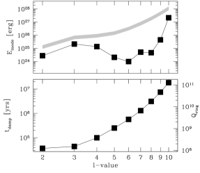
Figure 1.— F-modes and the rings. The top panel shows the mode energies as inferred from ring seismology, as a function of spherical degree (also see Table 1). The grey curve indicates the energy value at which the ring density wave will have reached unity amplitude. The bottom panel shows the damping time-scale for f-modes as they excite density waves in the C-ring, with the right axis approximately marking the corresponding quality factor. By contrast, internal damping typically give $Q\geq 10^{14}$.

While amplitudes of the associated density waves ($\Delta\Sigma/\Sigma$) have a spread of a factor of $10$, mode energies have a much larger spread, ranging from $10^{24}\,\rm erg$ to $10^{27}\,\rm erg$, with the $\ell=10$ mode having the highest energy. There is a characteristic mode energy at which ring waves become unity amplitude ($\Delta\Sigma/\Sigma=1$). These are indicated in Fig. 1. The $\ell=2,3$ and possibly the $\ell=10$ modes are close to this limit. In fact, visual inspections of the optical depth profile (Hedman & Nicholson, 2013) associated with the $\ell=2$ and $3$ waves would argue that they are above unity. Here, we assume that the damping rates for the f-modes are not strongly affected by this nonlinearity.

4. Internal Damping Are Weak

We consider various energy sinks for the f-modes inside Saturn. These include mode damping by radiative diffusion (near the photosphere where the thermal timescale is the shortest), by leakage of mechanical energy (into the isothermal stratosphere above the photosphere), and by viscosity associated with the turbulent convection (throughout the planet). We show that all of these yield $Q\sim 10^{14}$ or higher, and cannot compete with the above discussed ring damping. Previous work has come to very different conclusions regarding internal damping (e.g. Markham & Stevenson, 2018). Because the correct damping is important for estimating the level of stochastic excitation (eq. 39), we spend much labour in this section. Readers who are more interested in the excitations can jump ahead to §5.

For an inviscid fluid, internal heat can be removed by heat diffusion and mechanical work,

$$dQ=TdS-pd\left({1\over\rho}\right)\,.$$ (16)

Energy in the pulsation is changed as described by, e.g., eq. (25.7) of Unno et al. (1989),

$${{dE}\over{dt}} = {d\over{dt}}\int_{0}^{M}dM({1\over 2}v^{2}+{1\over 2}\Phi+Q)$$ (17)

$$= \int_{0}^{M}dM\,{T{{dS}\over{dt}}-\int_{R_{s}}p{\mbox{\boldmath$v$}}\cdot d{\bf S}}\,,$$

where the latter is a surface integral evaluated at Saturn’s photosphere. For a pulsation that is nearly strictly periodic and adiabatic, i.e., a Lagrangian perturbation of a complex form $\delta p=|\delta p|e^{i\theta_{p}}e^{i\omega t}$, with $\omega=\omega_{r}+i\omega_{i}\approx\omega_{r}$ ($|\omega_{i}|\ll\omega_{r}$), over one cycle, it gains energy

$$\Delta E=\Delta E_{\rm rad}+\Delta E_{\rm leak}=\oint dt{{dE}\over{dt}}=$$

$${\pi\over\omega}\int_{0}^{M}dM\,{\rm Re}\left[\delta T^{*}{{d\delta s}\over{dt}}\right]-4\pi^{2}R_{s}^{2}{\rm Im}\left[\delta p^{*}\xi_{r}\right]_{R_{s}}\,,$$ (18)

where quantities in the last expression have shed their oscillatory time-dependencies after the time-integration. The first term ($\Delta E_{\rm rad}$) is due to damping by internal heat diffusion, and the second term ($\Delta E_{\rm leak}$) is due to leakage of mechanical energy to vacuum.

For a viscous fluid, the fluid equation of motion has an additional friction term,

$$\rho\ddot{\mbox{\boldmath$\xi$}}=-\mbox{\boldmath$\nabla$}p^{\prime}+{{\mbox{\boldmath$\nabla$}p}\over{\rho}}\,\rho^{\prime}-\rho\mbox{\boldmath$\nabla$}\delta\Phi+{\mbox{\boldmath$F_{\nu}$}},$$ (19)

where the viscous force

$${\mbox{\boldmath$F_{\nu}$}}=\mbox{\boldmath$\nabla$}\cdot\left(\rho\nu\mbox{\boldmath$\nabla$}{\dot{\mbox{\boldmath$\xi$}}}\right)\,.$$ (20)

In our case, the viscosity $\nu$ arises from turbulent convection. Over one cycle, the mode energy changes by

$$\Delta E_{\rm vis}=\oint dt\int d^{3}r\,{\dot{\mbox{\boldmath$\xi$}}}\cdot{\mbox{\boldmath$F_{\nu}$}}={\pi\omega{{\int d^{3}r\,\rho\nu\,\mbox{\boldmath$\nabla$}\mbox{\boldmath$\xi$}:\mbox{\boldmath$\nabla$}\mbox{\boldmath$\xi$}}}}\,.$$ (21)

The most rigorous way to obtain the corresponding quality factor $Q$ (eq. 14) is to solve the non-adiabatic f-mode eigenfunctions. In the following, we take the quicker path of estimating the magnitudes of $\Delta E_{\rm vis}$, $\Delta E_{\rm rad}$ and $\Delta E_{\rm leak}$. This is a delicate procedure, but it is ultimately more physically illuminating. We are able to show that the three dampings are all exceedingly weak ($Q\geq 10^{14}$).

For simplicity, we suppress the $\ell$-dependence of the f-modes as we are concerned only with low-$\ell$ modes. We further assume that all fractional Lagrangian perturbations are of the same order, $\delta\rho/\rho\sim\delta T/T\sim\delta F_{\rm rad}/F_{\rm rad}$. Saturn’s atmosphere is taken to be fully convective up to the photosphere, above which there is an isothermal stratosphere. This ignores possible stratification by the so-called ’moist convection’ (Ingersoll & Kanamori, 1995), or the putative sub-adiabatic zone as suggested by Guillot et al. (1994).

4.1. Turbulent Damping

The interior of Saturn is convectively unstable. Energy-bearing turbulent eddies, driven by thermal buoyancy, have a scale of order the local scale height, $H$, and a characteristic velocity obtained by $\rho v_{\rm cv}^{3}=F$, where $F$ is the internal cooling flux and $F\approx 2200\,\rm erg/\,\rm s/\,\rm cm^{2}$ for Saturn. Eddies in the so-called inertial range are also present as the energy-bearing eddies turn-over and cascade down in scale. Taking the kinematic viscosity of the form

$$\nu\sim v_{\rm cv}H\left[{1\over{1+(\omega\tau_{\rm cv}/2\pi)^{s}}}\right]\,,$$ (22)

with the factor in the square braket representing the reduction in viscosity when the typical convection turn-over time ($\tau_{\rm cv}=H/v_{\rm cv}$) is much longer than the mode period, and inertial-range eddies, as opposed to the more powerful energy-bearing eddies, dominate the viscous damping. Even at the photosphere where convection is the fastest, adopting $H\sim 30\,\rm km$, $\rho_{0}\sim 10^{-4}{\bar{\rho}}$, we find that $v_{\rm cv}\sim 300\,\rm cm/\,\rm s$, $\tau_{\rm cv}\sim 10^{4}\,\rm s$, and $\omega\tau_{\rm cv}\gg 1$. In the following, we adopt $s=2$ as is appropriate for a Kolmogorov turbulence spectrum (Goldreich & Nicholson, 1977), and find that $\omega\tau_{\rm cv}\gg 1$ throughout the planet and that damping is dominated by eddies in the surface scale height, with $\nu\sim F/(\omega^{2}\rho H)$ (see Wu, 2005, for more details). So eq. (21) yields

$$\Delta E_{\rm vis}\sim 4\pi^{2}R_{s}^{2}{F\over\omega}\left({{\xi_{r}}\over R_{s}}\right)^{2}\sim{{\pi L_{\rm umin}}\over\omega}\left({{\xi_{r}}\over R_{s}}\right)^{2}\,.$$ (23)

where $L_{\rm umin}=4\pi R_{s}^{2}F$ is Saturn’s intrinsic luminosity. Scalings in §2 imply that $E_{\rm mode}\sim 0.5\omega^{2}M_{s}R_{s}^{2}(\xi_{r}/{\tilde{\xi}_{r}})^{2}$, so

$$Q_{\rm vis}={{E_{\rm mode}}\over{\Delta E_{\rm vis}}}\sim 10^{14}\left({{\omega}\over{10^{-3}\,\rm s^{-1}}}\right)^{3}\,.$$ (24)

4.2. Radiative Diffusion

Here, we consider heat diffusion by radiation between fluid parcels of different temperatures. In principle, convection can also thermally respond to pulsation and leads to further heat diffusion. But we ignore convection here because, first, there is no good first-principle treatment of perturbed convective flux; and second, the convection turn-over time is very long compared to the mode period and hence we may be justified to ignore its perturbations. Most of the diffusive heat-loss comes from the scale height just below the photosphere, where the diffusion time is the shortest. This is also where the convective flux is rapidly substituted by radiative flux, so $F=F_{\rm rad}+F_{\rm cv}\sim F_{\rm rad}\sim(4acT^{4})/(3\kappa\rho)d\ln T/dr$, and $dF_{\rm rad}/dr\sim F/H$, where $H$ is the local scale height.

The equation of energy conservation reads,

$$T{d{\delta s}\over{dt}}=-\delta\left({1\over\rho}\mbox{\boldmath$\nabla$}\cdot{\mbox{\boldmath$F$}}\right)\,.$$ (25)

Ignoring the perturbation to the convective flux, we set $\delta F=\delta F_{\rm rad}$ and expand the right-hand side in Lagrangian variables as

$$\delta\left({1\over\rho}\mbox{\boldmath$\nabla$}\cdot{\mbox{\boldmath$F$}}\right) = -{1\over\rho}{{\delta\rho}\over{\rho}}\mbox{\boldmath$\nabla$}\cdot{\mbox{\boldmath$F$}}+{1\over\rho}{{\delta\rho}\over{\rho}}\mbox{\boldmath$\nabla$}\cdot{\mbox{\boldmath$F$}}$$ (26)

$$+{1\over\rho}{d\over{dr}}\left({{\delta F_{\rm rad}}\over{F_{\rm rad}}}\right)F_{\rm rad}+{1\over\rho}{{\delta F_{\rm rad}}\over{F_{\rm rad}}}{{dF_{\rm rad}}\over{dr}}$$

$$\sim {F\over{\rho H}}{{\delta F_{\rm rad}}\over F_{\rm rad}}\,.$$

The term that involves $dF_{\rm rad}/dr$ dominates on the right-hand-side, since for f-modes, $\delta F_{\rm rad}/F_{\rm rad}\sim\delta\rho/\rho$ varies much more smoothly (see Fig. 2). Most of the contribution to damping comes from the scale height immediately below the photosphere, where the entropy perturbation is the largest (eq. 25). And we find

$$\Delta E_{\rm rad} = {\pi\over{\omega}}\int_{0}^{M}dM\,{\rm Re}\left[\delta T^{*}{{d\delta s}\over{dt}}\right]$$ (27)

$$= {\pi\over\omega}\int_{0}^{M}dM\,{\rm Re}\left[\left({{\delta T}\over T}\right)^{*}\delta({1\over\rho}\mbox{\boldmath$\nabla$}\cdot{\mbox{\boldmath$F$}})\right]$$

$$\sim {{\pi L_{\rm umin}}\over{\omega}}\left({{\delta\rho}\over{\rho}}\right)^{2}\,,$$

Because f-modes are highly incompressible, $\delta\rho/\rho\ll\xi_{r}/r$ (see Fig. 2), this term is much smaller than damping by turbulent viscosity (eq. 23).

We quantify the compressibility by

$${\cal F}\equiv{{\left|{{\delta\rho}\over\rho}\right|}\over{\left|{\xi_{r}}\over{r}\right|}}\ll 1\,,$$ (28)

evaluated near the surface. Following Markham & Stevenson (2018), we introduce the radiation constant $\tau_{\rm rad}\approx c_{p}T/\kappa F$. This is of order $\tau_{\rm rad}\sim 10^{7}\,\rm s$ at Saturn’s photosphere, defined as where $\kappa\rho_{0}H\sim 2/3$. Value for the surface scale height is $H\sim 30$km, and the photospheric density $\rho_{0}\sim 10^{-4}{\bar{\rho}}$, with ${\bar{\rho}}$ being the mean density of Saturn. We can now recast our result in their notation as

$$Q_{\rm rad} = {{E_{\rm mode}}\over{\Delta E_{\rm rad}}}$$ (29)

$$\sim (\omega\tau_{\rm rad})\left({\omega\over{\omega_{\rm dyn}}}\right)^{2}\left({{\bar{\rho}}\over{\rho_{0}}}\right)\left({{R_{s}}\over{H}}\right)^{2}{\cal F}^{-2}$$

$$\sim 10^{13}\left({{\omega}\over{10^{-3}\,\rm s^{-1}}}\right)^{3}{\cal F}^{-2}\,,$$

where $\omega_{\rm dyn}=\sqrt{G{\bar{\rho}}}\sim g/R_{s}$.

4.3. Wave Leakage

This is the most subtle damping to estimate. Material above the photosphere also oscillates and can in principle communicate the wave energy to infinity (or steepen into a shock at some height). For adiabatic oscillations, there is exactly zero leakage for waves with frequencies below the so-called acoustic cutoff frequency. This is true for all f-modes of concern. However, this is modified when entropy perturbation is considered (non-adiabatic perturbations). Our calculation below argues that $Q_{\rm leak}\gg 10^{13}$. In contrast, Markham & Stevenson (2018) found that $Q_{\rm leak}\sim 10^{7}$.

We assume the layer above the photosphere to be isothermal, as suggested by observation. So the scale height $H=\Gamma_{1}p/g\rho=-\Gamma_{1}d\ln p/dr$ remains largely constant. Here, the adiabatic index $\Gamma_{1}=(\partial\ln p/\partial\ln\rho)_{s}$. We first consider adiabatic perturbations before turning toward non-adiabaticity.

To obtain the wave characteristics at the photosphere and above, we adopt the form of adiabatic perturbation equation as in eq. (8) of Goldreich & Wu (1999),

$${{d^{2}}\over{dr^{2}}}\left({{\delta p}\over p}\right)-{{\Gamma_{1}}\over{H}}{d\over{dr}}\left({{\delta p}\over p}\right)+\left[k_{h}^{2}({{N^{2}}\over{\omega^{2}}}-1)+{{\omega^{2}}\over{c_{s}^{2}}}\right]=0\,.$$ (30)

Here, $k_{h}^{2}=\ell(\ell+1)/r^{2}$, the Brunt-Väisälä   frequency $N^{2}=g(d\ln\rho/dr-1/\Gamma_{1}d\ln p/dr)=(\Gamma_{1}-1)g/H$, and $c_{s}^{2}=\Gamma_{1}p/\rho=gH$. As all coefficients are constants on scale of $H$, the solution has the form $\delta p/p\propto\exp(k_{r}r)$, where

$$k_{r}={1\over 2}{{\Gamma_{1}}\over{H}}\pm{1\over 2}\sqrt{\left({{\Gamma_{1}}\over H}\right)^{2}-4\left[k_{h}^{2}({{N^{2}}\over{\omega^{2}}}-1)+{{\omega^{2}}\over{c_{s}^{2}}}\right]}\,.$$ (31)

The term in the square bracket is negative when $\omega\geq\omega_{\rm ac}=\Gamma_{1}c_{s}/2H$, where $\omega_{\rm ac}$ is the so-called acoustic cut-off frequency. In this case, the mode is propagative into the isothermal layer and it is strongly damped by wave leakage. On the other hand, when $\omega<\omega_{\rm ac}\sim 0.017\,\rm s^{-1}$ (or a period of $370\,\rm s$), as is the case of all f-modes we are concerned with, propagation is forbidden and the wave is evanescent in the isothermal layer. All energy flux is reflected back to and contained within the planet (Unno et al., 1989).

For the latter waves, causality dictates that one has to take the negative sign branch in eq. (31), because otherwise the energy density ($\rho\xi_{r}^{2}$) will rise exponentially with height. This leads to

$$k_{r}\approx{{k_{h}^{2}({{N^{2}}\over{\omega^{2}}}-1)+{{\omega^{2}}\over{c_{s}^{2}}}}\over{\Gamma_{1}/H}}\sim{\cal O}({1\over R_{s}})\,,$$ (32)

or that fluid displacements, as well as Lagrangian perturbations, can only vary on the scale of the planet radius. The nearly constant $\xi_{r}$, for instance, indicates both that the whole atmosphere is lifted up in unison, and that the energy density $\rho\xi_{r}^{2}$ decays exponentially with height. So the isothermal atmosphere reflects all energy density back into the interior. In other words, since the atmosphere communicates across with the speed of sound, for perturbations that vary more slowly than the acoustic cut-off, the atmosphere remains hydrostatic and cannot provide a restoring force.

The above conclusion is modified when radiative diffusion interferes. The perturbations, now no longer adiabatic, experience a phase shift between $\delta p/p$ and $\xi_{r}$. This introduces wave leakage. We estimate the magnitude of this effect.

Let the photospheric pressure be $p_{0}$,

$${\rm Im}\left[\xi_{r}^{*}\delta p\right]_{R_{s}}\approx R_{s}p_{0}\left.\left({{\xi_{r}}\over{r}}{{\delta p}\over p}\right)\right|_{R_{s}}\times(\delta\theta)\,,$$ (33)

where the difference in phases between the complex $\delta p/p$ and $\xi_{r}$, $\delta\theta$, is caused by changes in entropy,

$$-\mbox{\boldmath$\nabla$}\cdot\mbox{\boldmath$\xi$}={{\delta\rho}\over{\rho}}={1\over{\Gamma_{1}}}{{\delta p}\over p}+\rho_{s}\delta s\,.$$ (34)

Here $\rho_{s}=(\partial\ln\rho/\partial s)_{p}$. The entropy perturbations, in term, is related to flux retention (eq. 25), which, for an isothermal atmosphere where $dF_{\rm rad}/dr=0$ applies, is dominated by the third term on the right-hand-side of eq. (26). This produces

$$i\omega T\delta s\sim{1\over\rho}{d\over{dr}}\left({{\delta F_{\rm rad}}\over{F_{\rm rad}}}\right)\sim k_{r}{F\over\rho}{{\delta\rho}\over{\rho}}\sim{F\over{R_{s}\rho}}{{\delta\rho}\over\rho}\,.$$ (35)

Compared to the magnitude of $\delta s$ in the underlying convection zone, this value is smaller by a factor of $H/R_{s}$. This difference arises because of the isothermal structure of the atmosphere, as well as eq. (32). This leads to a rough estimate for the phase shift as

$$\delta\theta\sim{H\over{R_{s}}}{1\over{\omega\tau_{\rm rad}}}\,,$$ (36)

And an order of magnitude estimate for $Q_{\rm leak}$ is

$$Q_{\rm leak} \approx (\omega\tau_{\rm rad})\left({\omega\over{\omega_{\rm dyn}}}\right)^{2}\left({{\bar{\rho}}\over{\rho_{0}}}\right)\left({R_{s}\over H}\right)^{2}{\cal F}^{-2}$$ (37)

$$\sim 10^{13}\left({{\omega}\over{10^{-3}\,\rm s^{-1}}}\right)^{3}{\cal F}^{-2}\,.$$

This, interestingly, is of the same order of magnitude as that by radiative diffusion (eq. 29). It reflects the fact that both dampings scale with the internal flux, and both occur within a scale height of the photosphere. Both of these damping are much weaker than that by turbulent convection (eq. 24), because f-modes are very incompressible (${\cal F}\ll 1$).

4.4. Difference from Markham & Stevenson (2018)

Markham & Stevenson (2018) considered the same physics of wave leakage. But their approach led them to conclude a $Q_{\rm leak}$ of the form (their eq. 61)

$$Q_{\rm leak,MS} \approx (\omega\tau_{\rm rad})\left({\omega\over{\omega_{\rm dyn}}}\right)^{2}\left({{\bar{\rho}}\over{\rho_{0}}}\right)$$ (38)

$$\sim 10^{7}\left({{\omega}\over{10^{-3}\,\rm s^{-1}}}\right)^{3}\,.$$

This implies a dissipation orders of magnitude stronger than our estimate in eq. (37), with the difference being $(R_{s}/H)^{2}{\cal F}^{-2}\gg 10^{6}$. There are three reasons for this difference. First, while considering the Lagrangian pressure perturbation (their eq. 52), they equate $\delta p/p$ to $T^{\prime}/T$, where $T^{\prime}$ is the Eulerian temperature perturbation, while we equate $\delta p/p$ to $\delta T/T$. Because of the large temperature gradient near the surface (variation scale $H\ll R_{s}$), $T^{\prime}/T=\delta T/T-\xi_{r}dT/dr\approx(R_{s}/H)\delta T/T$, this brings about the first factor of $R_{s}/H$ in the difference. Second, we find that the wave is evanescent in the isothermal region. This leads us to adopt an entropy variation that is smaller than that in the convection zone below by a factor of $H/R_{s}$ (see discussion around eq. 35). Lastly, we argue that the incompressibility of f-modes should introduce a factor of ${\cal F}^{-2}$ into the calculation of $Q$.

5. Mode excitation: Convection and Storms

In this and the next sections, we will discuss plausible excitation mechanisms. As the modes appear to be stalled at amplitudes that are very weak, the most likely driving is stochastic in nature. In the presence of an external damping, stochastic forcing increases mode energies linearly in time, capped by the equipartition value ($E_{k}$),

$$E_{\rm mode}={\rm Max}\left\{N\Delta E_{\rm kick},E_{\rm k}\right\}\,,$$ (39)

Here $N$ is the number of discreet kicks received within the mode’s damping time, $\Delta E_{\rm kick}$ the typical energy given to the mode during one stochastic event, and $E_{k}$ the total energy of such an event. The capping reflects the fact that while the event can excite a mode, it can also absorb energy from the mode. According to the fluctuation-dissipation theorem, equipartition is the best possible outcome. Typically, $\Delta E_{\rm kick}\ll E_{k}$.

We argue above that the main damping for f-modes is via density waves in the rings, as opposed to any other dissipation internal to Saturn. This provides the requisite damping timescales. Here, we first focus on two previously proposed excitation mechanisms.

5.1. Convection

While there have been claims in the literature that turbulent convection can excite Saturn’s f-modes to the observed amplitudes (Marley, 1991; Marley & Porco, 1993; Fuller, 2014; Mankovich et al., 2018), this is in fact incorrect.

Due to the small intrinsic flux of Saturn, turbulent convection is far too weak (in velocity) and too slow (in turn-over time) to account for the observed mode energies—even in the absence of ring damping.

Stochastic excitation by fluctuating convective eddies occurs at a rate (Goldreich & Kumar, 1990; Goldreich et al., 1994; Markham & Stevenson, 2018)

$$\left.{{dE}\over{dt}}\right|_{\rm cv}\sim 2\pi\omega^{2}\int_{0}^{R_{s}}dr\,r^{2}\rho^{2}\left|{{d{\tilde{\xi}_{r}}}\over{dr}}\right|^{2}\int_{0}^{h_{\omega}(r)}{{dh}\over h}v_{h}^{3}h^{4}\,,$$ (40)

where $v_{h}$ and $h$ are the eddy velocity and size, respectively. Only eddies that turn-over faster than the mode period contributes, or, $h\leq h_{\omega}$ where $h_{\omega}$ is the largest eddies for which $(h/v_{h})\sim 1/\omega$. These eddies are all in the inertial range, since the energy-bearing eddies satisfy $\omega\tau_{\rm cv}=\omega H/v_{\rm cv}\gg 1$, everywhere inside Saturn. For a Kolmogorov turbulent spectrum, $v_{h}\sim(h/H)^{1/3}v_{\rm cv}$, so we only need be concerned with $h\sim h_{\omega}$ and the stochastic driving rate is

$$\left.{{dE}\over{dt}}\right|_{\rm cv}\sim 2\pi\omega^{2}\int_{0}^{R_{s}}dr\,r^{2}\rho^{2}\left|{{d{\tilde{\xi}_{r}}}\over{dr}}\right|^{2}v_{\omega}^{3}h_{\omega}^{4}\,,$$ (41)

where the velocity at $h_{\omega}$ is $v_{\omega}$ and we have $v_{\omega}=\omega h_{\omega}$, and $h_{\omega}=H\left(1/\omega\tau_{\rm cv}\right)^{3/2}$. This integral is dominated by the contribution from the top scale height.

In the mean time, turbulence removes energy from the modes in the form of turbulent viscosity (eq. 21). The kinematic viscosity in eq. (22) can be manipulated to become the following form

$$\nu\sim v_{\omega}h_{\omega}\,.$$ (42)

Or, viscous damping is dominated by the same eddies that drive the modes.

When the stochastic driving and damping are balanced, we reach the so-called ’fluctuation-dissipation’ equilibrium, or ’energy equipartition’. Both driving and damping are dominated by turbulent eddies near the surface, since $\omega\tau_{\rm cv}$ is the smallest there and the relevant eddies ($h_{\omega}$) lie closest to the energy-bearing eddies. Equating the driving in eq. (41) with the damping from eq. (23), we find that mode energy is equilibrated to that of the relevant eddy,

$$E_{\rm mode}\sim\rho v_{\omega}^{2}h_{\omega}^{3}\,.$$ (43)

Evaluating near the surface, we find

$$E_{\rm mode}\sim 5\times 10^{14}\,\rm erg\left({{\omega}\over{10^{-3}\,\rm s^{-1}}}\right)^{-11/2}\,.$$ (44)

Due to the steep dependence of the above expression on frequency, any missing factors of $2$ or $\pi$ can dramatically affect the result. To be be cautious, we calibrate our results against that obtained for the Sun. The most highly excited modes in the Sun are observed to have energies of order $10^{28}$ ergs, at frequencies of $3$ mHz, or $\omega\sim 0.02\,\rm s^{-1}$. Equation (43) implies a physical scaling

$$E_{\rm mode}\propto{{F^{5/2}}\over{\rho^{3/2}H^{5/2}\omega^{11/2}}}\,.$$ (45)

The solar photosphere has $\rho\sim 2\times 10^{-6}\,\rm g/\,\rm cm^{3}$, scale height $H\sim 30\,\rm km$, and flux $F=7\times 10^{10}\,\rm erg/\,\rm s/\,\rm cm^{2}$. Substituting these into the above equation, we find that $E_{\rm mode}$ in Saturn should be some $10^{-15}$ smaller than that in the Sun. This confirms our result in eq. (44). Moreover, the predicted $E_{\rm mode}$ drops sharply with mode frequency, as is also observed for solar p-modes with frequencies above $3$ mHz.

Eq. (44) falls below by orders of magnitudes compared to that found by Markham & Stevenson (2018). They concluded that, for Jupiter, f-mode energies by turbulent convection should be only $3$ orders smaller than those in the Sun. Unfortunately, we fail to reconstruct their results and so could not resolve our differences.

Eq. (44) lies much below the f-mode energies inferred from ring seismology (Table 1). This excludes turbulent convection as a plausible source of excitation. The situation is further exacerbated by the fact that Saturn’s rings damp the f-modes much more strongly than internal dissipation. Eq. (39) suggests that in this case,

$$E_{\rm mode}\sim 5\times 10^{14}\,\rm erg\left({{\omega}\over{10^{-3}\,\rm s^{-1}}}\right)^{-11/2}\left({{Q_{\rm ring}}\over{Q_{\rm vis}}}\right)\,.$$ (46)

5.2. Water Storms, Rock Storms…

In the presence of trace volatiles, convection can take a more complicated form. Other than the quasi-equilibrium turbulent convection studied above, there could be episodic, triggered convection that is driven not by the small super-adiabatic gradient, but by the latent heat release from the condensing volatile. Such “storm” cells are observed on the surface of Jupiter (Gierasch et al., 2000) and Saturn (Sayanagi et al., 2013), and when they occur, can carry a fair fraction of the internal flux, ranging from a few percent on Saturn (Li et al., 2015), to $\sim 60\%$ on Jupiter (Gierasch et al., 2000). Deeper storms (’rock storms’), possibly driven by the condensation of refractory material (silicate, magnesium, iron-bearing) has also been hypothesized to exist much deeper inside the planet (up to $10^{4}$ bars). Markham & Stevenson (2018) considered whether these storms can excite f-modes in Jupiter(also see Dederick et al., 2018). They argued that shallow water storms are too weak to be relevant, but introduced the ingenious idea of a rock storm. We re-evaluate their hypothesis here.

Updraft of a warm, moist parcel (water or silica) can hit into the cloud layer on top, depositing its momentum and energy. Analogous to the effects of an external impact, this can excite f-modes (see section below). While storms on Earth, Jupiter, and Saturn are observed to have a horizontal extent of order thousands of kms, here we assume that only a spherical patch of order the local scale height can act as an impulse in driving the modes. Time coherence across different such patches is likely weak and can be considered as random, uncorrelated punches (Markham & Stevenson, 2018).

Following (Markham & Stevenson, 2018), relevant physical parameters for the water storms and the (hypothetical) rock storms are listed in Table 2. In particular, the storm energy is

$$E_{k}\sim\rho_{0}H^{3}v_{\rm storm}^{2}\,,$$ (47)

where the storm velocity is related to the buoyancy acceleration $v_{\rm storm}^{2}\sim(fL_{v}/c_{p}T)gH$, with $L_{v}$ being the latent heat for the volatile and $f$ the volatile mass fraction. We adopt the latter to be about $10$ times solar, for both the water and the rock cases. As Table 2 shows, these storm cells contain orders of magnitude more energy than that in a quasi-equilibrium turbulent cell that has the same frequency as an f-mode (eq. 44).

Table 2Storms and f-mode excitation

	’ice storm’	’rock storm’
depth ($H$)	$30\,\rm km$	$10^{8}\,\rm cm$
density ($\rho_{0}$)	$10^{-4}{\bar{\rho}}$	$0.05{\bar{\rho}}$
latent heat	$2.3\times 10^{10}\,\rm erg/g$	$1.2\times 10^{11}\,\rm erg/g$
volatile mass fraction	$5\%$	$1\%$
buoyancy speed ($v_{\rm storm}$)	$10^{4}\,\rm cm/\,\rm s$	$3\times 10^{4}\,\rm cm/\,\rm s$
energy in one storm cell ($E_{k}$)	${{10^{24}}}$ergs	$10^{32}\,\rm erg$s
one-kick energy ($\Delta E_{\rm kick}$, $\ell=2$)	$10^{6}\,\rm erg$s	${10^{22}}$ergs

Let us take the simplistic picture that the condition conducive for the storm builds up gradually, and then within a time short compared to the f-mode period the entire storm cell releases the latent heat contained within. A shallow water storm has energy comparable to that of an $R=30\,\rm m$ impactor, while the deep rock storm is equivalent to that of an $R=15\,\rm km$ impactor. Using algebra similar to that for an meteor impact (eq. A9), we find that the one-kick energy, $\Delta E_{\rm kick}$, for the $\ell=2$ f-mode, is $10^{6}$ ergs for the water storm and $10^{22}$ ergs for the rock storm, These values grow with the mode’s spherical degree as $\ell(\ell+1)$.

We can exclude water storms as an important source of driving. Requiring that the $\ell=2$ mode be excited to its observed value, $E_{\rm mode}=3\times 10^{24}\,\rm erg$, within its damping time of $\sim 4\times 10^{4}$yrs, one finds that the water storms need to occur very frequently and transport a flux that is some $10^{6}$ times higher than Saturn’s total flux. In addition, energies in the higher-$\ell$ modes actually exceed the equipartition value.

The rock storms, on the other hand, are less conclusive. The same exercise for the $\ell=2$ mode shows that they only have to carry some $2\%$ of the internal flux, and occur once every century. At the moment, we do not know if such deep storms exist, let alone their frequency. So such a scenario cannot be excluded, or substantiated.

6. Mode excitation: Impacts

F-modes in Saturn have life-times that range from $4\times 10^{4}$ yrs to $2\times 10^{7}$ yrs. Could large impacts that occur over these timescales be responsible for exciting the f-modes to their current amplitudes? In other words, could Saturn still be trembling from terrors of the deep past?

6.1. Bombardment Rates on Saturn

We first summarize observations on direct impacts onto Saturn. Zahnle et al. (2003) compiled impact rates on outer solar system bodies, as a function of impactor size. These are based on impact crater counts on the moons of the giant planets, and on the observed populations of Kuiper Belt objects. For Saturn, they found that an impactor of radius $R=1\,\rm km$ arrives once every $\sim 100$ yrs, while $R=100\,\rm km$ bodies arrive once every $\sim 10^{8}$ yrs. Impact rates in their Fig. 2 can be roughly fit by a power-law,

$$\gamma_{imp}(R)\approx 10^{-2}\left({{R\over{1\,\rm km}}}\right)^{-2.8}{\rm\,yr}^{-1}\,.$$ (48)

Such a scaling implies that the mass flux (and energy flux) is roughly flat with impactor size. Uncertainties in these rates are listed at about an order of magnitude. Moreover, the size distribution of Kuiper Belt objects is not a simple power-law but contains structures. So this fit is a simplification.

Jupiter, being more massive, sustains a bombardment rate some $2.5$ times larger.

6.2. Energy Imparted to Normal Modes

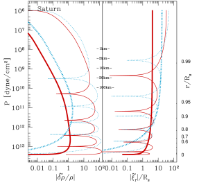
Figure 2.— Normalized eigenfunctions for a few fundamental- and p-modes in Saturn. The red (or solid) lines are for the $\ell=2$ modes and the blue (or dotted) for $\ell=10$; heavy lines represent f-modes, while thin lines the $n=5$ radial overtone p-modes. Mode excitations by impacts are directly proportional to the heights of the eigenfunctions here, with the explosion driving related to the fractional Lagrangian density perturbation (left panel), and the momentum punch related to the radial displacement (right panel). Legends in the middle indicate the approximate stopping depths for impactors of various radii.

Figure 3.— Mode amplitudes (in terms of surface radial displacements, top panels) and energies (bottom panels) excited by an impactor of radius $R=10\,\rm km$ (left) and one of $R=100\,\rm km$ (right), entering at the pole. F-modes are shown as solid circles and p-modes as open circles with smaller sizes indicating higher radial overtones.

Inspired by the impact of comet Shoemaker-Levy 9 onto Jupiter, Zahnle & Mac Low (1994) simulated a 1-km body colliding with Jupiter at the escape speed. There is a rich phenomenology (penetration, airburst, backward outflow, fireball, chemistry…), but here we focus only on two aspects that are of relevance to f-mode excitation.

As the body plows into the planet, it is rapidly decelerated to a halt after encountering material of a column density roughly comparable to itself (Fig. 1 of Zahnle & Mac Low, 1994). There it deposits most of its kinetic energy. The resulting heating causes an initially supersonic expansion that quickly transitions to subsonic in all directions, except perhaps for the upwards direction. Much of the over-pressure from the initial fireball dissipates gradually over the much longer thermal timescale. The impactor also deposits its downward momentum at the same location. Here, we make the optimistic assumption that the heated bubble contains all of the impact energy as well as all of the impact momentum.

Impacts can excite oscillations in two ways. First, the nearly instantaneous jump in gas pressure excites oscillations. This can be studied either by using the over-pressure as a forcing function on an eigen-mode (Lognonne et al., 1994; Dombard & Boughn, 1995), or by linearly decomposing the over-pressure signal onto a basis of eigenfunctions. We follow the first approach here. Second, the momentum delivery also exerts a force on the fluid and drives oscillations (Kanamori, 1993; Lognonne et al., 1994; Dombard & Boughn, 1995). We call the former ’explosion’ excitation, and the latter ’momentum punch’. In the Appendix, we follow Lognonne et al. (1994); Dombard & Boughn (1995) in deriving these two kinds of excitations, Figure 3 shows the result produced by impactors of two different sizes, after summing energy gains from both mechanisms. In the following, we provide a qualitative description.

Fundamental modes are surface gravity-waves with most of their energies stored in kinetic and gravitational potential, and only a small fraction in compression (Fig. 2). As is shown by Fig. 2, they are largely incompressible with

$${{\delta\rho}\over{\rho}}\ll{{\xi_{r}}\over{R_{s}}}\,.$$ (49)

So they are primarily excited by the momentum punch mechanism. P-modes, on the other hand, are compressive and can be effectively excited also by the explosion mechanism.

Following eq. (A9) and eq. (5), the energy imparted to a mode due to the momentum punch of an impactor entering at escape velocity is

$$E_{\rm mode} = {{\sqrt{\ell(\ell+1)}}\over 2}{{GM_{s}^{2}}\over{R_{s}}}\times a_{\rm punch}^{2}$$ (50)

$$\sim \left[\ell(\ell+1){{E_{\rm impact}}\over{E_{\rm grav}}}\right]E_{\rm impact}\,,$$

where $a_{\rm punch}$ is the dimensionless amplitude excited by the punch. Here, $E_{\rm impact}$ is the impactor’s gravitational energy and $E_{\rm grav}$ is Saturn’s binding energy, $GM_{s}^{2}/R_{s}$.

Higher-$\ell$ modes are more strongly excited because they live closer to the surface where the impact occurs. This trend is reversed at $\ell\geq 100$, as can be observed in the right panels of Fig. 3. This is related to the penetration depth of the impactor. A large impactor can deposit most of its momentum at a large depth, below where high-$\ell$ f-modes have the largest displacements. A similar behaviour is also observed for acoustic modes (radial order $n>0$). Impact excitation initially rises with $n$ because these modes are more superficial. But by the time $n$ is above a few, their first nodes lie shallower than the impact depth, and their eigenfunctions oscillate over the impact region. Impact forcing cancels to a large degree. We model this effect using the simplistic eq. (A10).

The scaling in eq. (50) also shows that larger impactors are more efficient in exciting the oscillations.

Mode energies scale steeply with impactor mass ($M$) and radius ($R)$ as

$$E_{\rm mode}\propto M^{2}\propto R^{6}\,.$$ (51)

Such a scaling can be observed by comparing the left and right panels in Fig. 3. In our calculations that include modes up to $\ell\sim 150$, the smaller impactor converts some $3\%$ of its total energy into normal modes, while the larger one converts $500\%$. The latter efficiency, exceeding unity, reflects the failure of our procedure in cutting off high order, high degree modes (eq. A10). Moreover, these modes have such high frequencies, it is no longer possible to imagine that the impact forcing is a delta-function in time.

We have also made a number of other simplification o produce results in Fig. 3. We assume that the impact arrives radially at the pole. So only the zonal modes (azimuthal quantum number $m=0$) are excited. Reality is more complicated: the rotation axis can be different from the impact axis, and the impact can be off-centre. Both give rise to a spread in mode energies between modes with the same $n$ and $\ell$ quantum numbers, but different $m$ values.

In summary, only a finite number of modes are effectively excited by the impact, and larger impactors are more efficient in driving these modes.

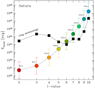
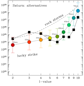
Figure 4.— Energies of f-modes in Saturn. Mode energies derived from ring seismology are shown as solid squares. Color circles in the left panel present energies expected from the largest impact that arrive within a mode’s lifetime, with small texts indicating the approximate radii of the responsible impactor, and error-bars reflecting a factor of $\sqrt{10}$ uncertainty in impact rates either way. Impact theory can explain high-$\ell$ modes, but fail by about a factor of $1000$ for the three lowest-$\ell$ modes. To reconcile this, we present in the right panel outcomes from two alternative scenario, one (lucky strike, color circles) in which a large body ($R=25\,\rm km$) hit within the past $40,000$ yrs; the other (’rock storms’, grey dashed curve) where deep-seated storms inside Saturn is responsible for exciting the f-modes. The storms are assumed to carry $2\%$ of the internal flux.

6.3. Exciting f-modes in Saturn

We now proceed to estimate mode energies excited by past impacts on Saturn.

According to the observed size spectrum (eq. 48), impactors bring in roughly equal energy flux per logarithmic size decade. In the mean time, larger impactors are much more efficient at conducting their energy into the normal modes. So over a given time window, even though the largest impactors are the rarest, they contribute the most to exciting f-modes.

The relevant time window for a given mode is its lifetime. As high-$\ell$ modes are more long-lived, they have a longer memory of past impacts, and consequently, weightier ’largest impactors’. They should be excited to much higher energies. Combining eqs. (48), (50), & (51), as well as our previous result that $t_{\rm damp}\propto[\ell(\ell+1)]^{2}$, we obtain the following scaling

$$E_{\rm mode}\propto\ell(\ell+1)R^{6}\propto\ell(\ell+1)t_{\rm damp}^{6/2.8}\propto\ell^{10.6}\,.$$ (52)

Numerical results shown in Fig. 4 (left panel) bear out this scaling, with expected mode energies varying steeply from $10^{21}\,\rm erg$ for the $\ell=2$ mode to $10^{28}\,\rm erg$ for the $\ell=10$ mode. Impacts that are responsible for these modes (the largest impacts) range from $R\sim 8\,\rm km$ for the strongly damped $\ell=2$ mode, to $R\sim 76\,\rm km$ for the weakly damped $\ell=10$ mode.

Compared to the observed energies, our expectations are too low by about $3$ orders of magnitude for the lowest degree modes ( $\ell=2,3,4$), but lie somewhat above (and are therefore compatible with) those for the $\ell=5-10$ modes.

6.4. The Low-$\ell$ problem

Although the impact theory appears to be a partial success, its ability to explain the observed energies in modes of the lowest degrees is worrisome. This either implies an unknown source of excitation for these modes, or that some aspects in the impact theory are wrong. We briefly discuss a few possibilities here.

First, could the observed low-$\ell$ modes be the result of an unexpectedly large invader in the recent past? To raise their energies up by a factor of $10^{3}$ would require a body with size $R\sim 25\,\rm km$ (eq. 51), impacting Saturn within the past $40,000$ yrs. In contrast, such a body is expected to visit once every $10^{6}$ yrs (eq. 48). So this is a small (but not vanishingly small) probability event. And uncertainties in the impact rate (up to a factor of $10$) could mitigate some of the discrepancy. In the right-panel of Fig. 4, we present the outcome of such a ’lucky’ scenario. This appears to resolve much of the tension between theory and observation. The disadvantage of such suggestion is that it is hard to disprove.

Another possibility is that the mode damping timescale is incorrectly calculated. If the low-degree modes are damped much more weakly than we have calculated, they can have longer memories of past impacts and can be excited to larger amplitudes. It also happens that the density waves forced by the low-degree modes are nearly nonlinear, as is suggested by Fig. 1. Is it possible that nonlinear density waves are less efficient in transporting angular momentum and energy away from the resonant location than their linear counter-parts? Such a possibility is not favoured by theoretical calculations (Shu et al., 1985; Borderies et al., 1986), which argue that they are as efficient as would be expected from linear calculations.

Another suggestion is that low-$\ell$ modes may exchange energy with modes at higher energies. As Fig. 3 shows, impacts can excite a large number of f-modes and p-modes. The three f-modes of concern here, with $m=\ell\in[2,3,4]$, are special in that they are quickly damped by resonances with the rings. But they are embedded in a heat bath where other modes oscillate with much higher energies. If some process, e.g., scattering by convective eddies (Goldreich & Murray, 1994), or nonlinear mode coupling (Wu & Goldreich, 2001), can bring the modes toward energy equipartition, this could help explain the energy floor at $\sim 10^{24}\,\rm erg$ for the low-$\ell$ modes. Further investigations are needed.

Lastly, we return to the discussion on rock storms. As one such deep-seated storm releases an energy comparable to that of a $R=15\,\rm km$ impact (§LABEL:subsec:storm), over the lifetimes of the detected f-modes, they may pump enough energies to explain the observations. These are shown in the right panel of Fig. 4 as a grey dotted curve, under the assumption that the storms carry a few percent of Saturn’s internal luminosity (so as to reproduce the level in the $\ell=2$ mode). Whether such an assumption is physically motivated is not known.

So to summarize, we are left at an unsatisfactory state. There are a couple alternative scenarios but we have no means to distinguishing them.

7. Exciting Jupiter’s normal modes

Assuming that internal dampings are weak on Jupiter, as on Saturn, the absence of a massive ring around Jupiter brings about dramatic consequences for the impact excitation. Now, the bombardment history can be remembered for of order the modes’ internal damping times, which are longer than a billion years. We expect much larger mode amplitudes, ones that can be readily observed.

To illustrate, we consider a single impact of $R=150\,\rm km$, which has an arrival rate of $\sim 1/$Gyrs on Jupiter (Zahnle et al., 2003). Energies for some of the most excited modes are shown in Fig. 5 – they are much higher than the counterparts in Saturn. For such a large impactor, one expects that most of the impact energy and momentum are deposited at a pressure $p_{\rm imp}\sim 10^{10}$ cgs. This means acoustic modes with radial order $n\sim 3-6$ achieve the highest excitation. Modes at higher radial orders can propagate to above this depth, and their excitation suffers cancellation.

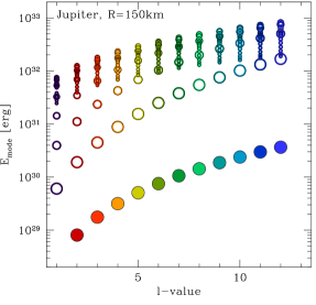
Figure 5.— Modes excited on Jupiter by a single $R=150\,\rm km$ impact. F-modes are shown as solid circles, and p-modes as open circles, with the circle size decreasing with radial order. The $\ell=1$ f-mode does not exist in nature. P-modes of radial order $n\sim 3-6$ acquire the highest energies.

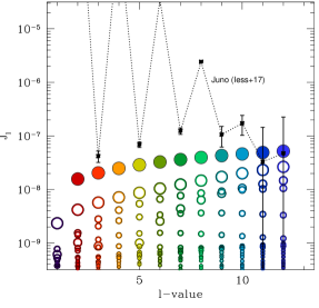
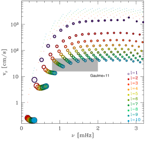
Figure 6.— Observable signatures, after an impact by a $R=150\,\rm km$ body on Jupiter. Symbols are the same as in Fig. 5. The left panel depicts the associated zonal ($m=0$) gravitational moments. Black points with error bars indicate Juno measurements for the static gravitational moments of Jupiter after a few crossings (Iess et al., 2018). The right panel displays the expected surface radial velocities, with small dots marking the maximum velocity amplitudes at surface, and circles those integrated over the visible disk (see text). The grey box marks the strength and frequency of detections sas reported by Gaulme et al. (2011).

In the following, we translate these energies into two observables: zonal gravitational moments, $J_{\ell}$ (eq. 7), potentially measurable by the Juno spacecraft currently orbiting Jupiter; and surface radial velocities $v_{r}$, detectable by ground-based spectroscopy (Mosser et al., 2000; Gaulme et al., 2011). The following results for $J_{l}$ and $v_{r}$ both scale with the impactor size as $R^{3}$.

The expected gravitational moments are shown in the left panel of Fig. 6. F-modes, being more deep-seated, dominate the signal, despite their lower energies. These are contrasted against current measurements. The static (zero-frequency) zonal moments of Jupiter have been measured down to a precision of order $10^{-8}$, after just a few swing-bys of the Juno spacecraft (Bolton et al., 2017; Iess et al., 2018). While the even order zonal moments ($J_{2},J_{4}...$) are large and are dominated by rotational flattening of Jupiter, the odd moments ($J_{3},J_{5}...$), likely caused by the surface zonal winds, have magnitudes of order $10^{-7}$. These are comparable to our estimates for the impact-excited f-modes. So the prospect is bright if a similar precision can be reached for the oscillating moments by analyzing the Doppler residual in Juno’s orbit(Durante et al., 2017). Different from the zonal winds, f-mode signatures are both time-dependent and may include tesseral moments ($m\neq 0$).

P-modes, instead of f-modes, dominate the radial velocity signal. We find that the maximum signal should lie around $1-3$ mHz, and feature p-modes of radial order $5-20$ (right-panel of Fig. 6). The maximum amplitudes on the surface of Jupiter can reach of order a few tens of metres per second, with higher-$\ell$ modes having larger amplitudes. However, when one observes the un-resolved Jupiter from the ground, the radial velocity signals are those projected along the line-of-sight, and averaged over the visible disk. For our order-of-magnitude exercise, we approximate these by dividing the maximum velocities by a factor of $\ell^{2}$, to account, crudely, for the cancellation between different light and dark patches. This exercise diminishes the signals for high-$\ell$ modes, and we predict that the radial velocities are now dominated by $\ell=1$ modes, peaking at $v_{r}\sim 10\,\rm m/\,\rm s$.

Using a dedicated radial velocity instrument and observing the solar Mg line at 517 nm reflected off Jupiter’s clouds, Gaulme et al. (2011) reported excess power on Jupiter, at frequencies between $0.8$ and $2.1$ mHz. and a possible secondary excess power between $2.4$ and $3.4$ mHz, just below the acoustic cut-off frequency at $3.5$ mHz. Encouragingly, these signals are modulated by a comb-like structure, resembling those of p-modes with $n=4-11$, and $\ell\sim 1$. The frequency and velocity amplitude they reported are crudely shown as a grey-box in Fig. 6, where the amplitudes are obtained using a $3\mu Hz$ window smoothing. Fitting the data using a single sine-wave (a delta-function in frequency), they set a limit of $50\,\rm cm/\,\rm s$ for a single mode.

So while the frequency and mode identity reported by Gaulme et al. (2011) appear consistent with what we expect from impact excitations, their maximum velocity is a factor of $\sim 20$ too low. Part of this may be related to our simplified, order-of-magnitude-level calculations, but a bigger part may be related to a problem we have not yet tackled – the internal damping of p-modes. These modes are compressible and propagate very close to the surface. They also have frequencies close to the acoustic cut-off. Mosser (1995) have studied this problem and argued that p-modes with frequencies between $1-2$ mHz are strongly damped by wave leakage with $Q\leq 10^{7}$. If this is indeed true, they can dramatically reduce our predicted amplitudes for these modes.

In summary, Jovian f-modes should be excited to levels likely detectable by the Juno mission, while impact-driven low-order p-modes may explain the radial velocity signals reported by Gaulme et al. (2011). More investigations are needed.

It is interesting to note that Saturn may also have detectable radial velocity signals – only a few f-modes have resonances in the rings and are thus strongly damped. Other modes should have much higher amplitudes.

8. Conclusions and Predictions

F-modes are excited in Saturn. They force density waves in Saturn’s rings that become visible in the Cassini stellar occultation data. We have obtained a number of theoretical results regarding the driving and damping of these modes:

1. the very density waves that reveal these oscillations remove energy from them on a timescale that ranges from $10^{4}$ to $10^{7}$ yrs;

2. in comparison, any other energy sink inside Saturn is negligible for these f-modes, with damping timescales that run upward of billions of years;

3. unlike convection in the Sun, turbulent convection in Saturn is too feeble to excite these modes to the observed level; so are surface storms that are driven by latent heat release of water (“water storms”); deeper storms that are possibly driven by the latent heat of refractive elements (“rock storms”) may be potent in driving these modes, but their existence and frequency remain unknown;

4. another source of stochastic excitation is impacts. The long damping times allow the modes to remember large impacts from eons ago. High-$\ell$ modes are excited to higher energies as they have longer memories. This theory adequately explains the observed amplitudes in the $\ell=5-10$ f-modes, but falls short for the lower-$\ell$ modes;

5. the low-$\ell$ modes may be excited by a fortuitously large recent impact; or a different mechanism (e.g., ’rock storms’); or energy exchange with other modes;

6. transcribing these processes to the case of Jupiter, which does not have a massive ring, suggests that Jupiter could still be vibrating from very large impacts that arrived billions of years ago; this opens the possibility of direct detection by the Juno spacecraft, and of explaining literature claims of ground-based detections.

There are many caveats and puzzles that we fail to resolve in this work. We list a few of them here, together with some predictions that may be tested in the near future:

• it remains a coincidence that f-modes in Saturn acquire just enough energy to excite visible features in Saturn’s C-rings. This would not have been possible if, e.g., the C-rings were a few times denser, or the impact rates were a few times lower.

• inferred surface displacements for all f-modes cluster around $1\,\rm m$. Is this a coincidence?

• density waves driven by low-$\ell$ modes are likely nonlinear. Could this influence our estimates for their lifetimes?

• impacts excite f-modes over a broad range of $\ell$ and $m$ values. They also excite acoustic modes. Only some of the f-modes, ones that find resonances within Saturn’s rings, are easily visible and are drained rapidly. The rest should have larger amplitudes and could be searched for either in the Cassini orbital data, or using radial velocity techniques from the ground.

• The acoustic modes will dominate the radial velocity signals. Our crude predictions for their amplitudes, in Saturn and in Jupiter, are based on the assumptions that they have lifetimes comparable to that of f-modes. This deserves further scrutiny. Detecting these modes is valuable because, compared to f-modes, they are more sensitive to the interior structure of the giant planets.

The Earth and Moon record past bombardments, in the form of craters on their surfaces. Giant planets can also remember their history, in the form of long-lived oscillations.

acknowledgement We wish to acknowledge discussions with Phil Nicholson, Matt Hedman, Peter Goldreich and Yuri Levin. WYQ thanks NSERC for research funding, YL acknowledges NSF grant AST-1352369 and NASA grant NNX14AD21G.

Appendix A Impact Excitation

To calculate the excitation of internal modes by impact, we adopt the derivations in Lognonne et al. (1994); Dombard & Boughn (1995), recapped here briefly.

Starting from the fluid equation of motion,

$$\rho{{d{\mbox{\boldmath$v$}}}\over{dt}}=-{\mbox{\boldmath$\nabla$}}P+\rho{\mbox{\boldmath$\nabla$}}\Phi+{\mbox{\boldmath$F$}}(\mbox{\boldmath$r$},t)\,$$ (A1)

where the last term represents the forcing related to the impactor, we decompose the forced response in terms of the free oscillation modes, ${\mbox{\boldmath$\xi$}}_{k}({\mbox{\boldmath$r$}})$,

$${\mbox{\boldmath$\xi$}}({\mbox{\boldmath$r$}},t)=\sum_{k}a_{k}(t){\tilde{}\mbox{\boldmath$\xi$}}_{k}({\mbox{\boldmath$r$}})\,,$$ (A2)

where the eigenfunctions are normalized as in eq. (2). In particular, the radial displacement for mode $k$ has the form

$${\tilde{\xi}}_{r}(\mbox{\boldmath$r$})={\tilde{\xi}}_{r}(r)Y_{\ell m}(\theta,\phi)\,,$$ (A3)

and the spherical harmonics function is normalized as $\int d\Omega Y_{\ell m}Y_{\ell m}^{*}=1$.

We can recast the equation of motion into the following simpler form

$${\ddot{a}}_{k}+\omega_{k}^{2}a(t)=F_{k}(t)\,,$$ (A4)

where

$$F_{k}(t)={{\int dV\,{\mbox{\boldmath$F$}}({\mbox{\boldmath$r$}},t)\cdot{\tilde{}\mbox{\boldmath$\xi$}}_{k}({\bf r})}\over{\int dV\rho(r){\tilde{}\mbox{\boldmath$\xi$}}_{k}\cdot{\tilde{}\mbox{\boldmath$\xi$}}_{k}}}\,.$$ (A5)

The response of the mode to a slowly varying forcing ($F_{k}(t)$) is facilitated by adopting a new variable that is slowly varying in time, $b_{k}(t)=a_{k}(t)e^{-i\omega_{k}t}$. This allows us to ignore ${\ddot{b}}_{k}$ and obtain

$$b_{k}(t)\approx-{{i}\over{\omega_{k}}}\int_{-\infty}^{\infty}F_{k}(t)e^{-i\omega_{k}t}dt\,.$$ (A6)

We now consider two possible forcings exerted by an impact, the over-pressure region after the impactor’s energy is converted into heat (’explosion’), and the momentum the impactor deposited at the envelope (’punch’). We make a number of simplifications to describe the temporal and spatial behaviours of the forcing. As the impactor travels fast and is braked after encountering a comparable amount of mass, the event only lasts $\Delta\tau\sim l/v\sim$ a few seconds, where $l$ is the penetration depth. So the first one can be thought of as a rapid deposition followed by a slow dissipation, as the local thermal time is long, or, roughly, a Heaviside step function ${\cal H}(t)$. The momentum punch, on the other hand, can be thought of as a top-hat function with duration $\Delta\tau$. Spatially, we assume that the explosion can be described as an over-pressure ($\delta P_{\rm expl}$) region at location ${\mbox{\boldmath$r$}}_{0}$ with a radius of $\Delta r$, and the total momentum ($\delta{\bf p}_{\rm punch}$) is deposited in the same region, both again approximated by the Heaviside function,

$${\mbox{\boldmath$F$}}_{\rm expl}(\mbox{\boldmath$r$},t) =-{\mbox{\boldmath$\nabla$}}\left\{{\delta P_{\rm expl}}\times{\cal H}\left[{{|{\mbox{\boldmath$r$}}-{\mbox{\boldmath$r$}}_{0}|}\over{\Delta r}}-1\right]\right\}\times{\cal H}(t)\,$$ (A7)

$${\mbox{\boldmath$F$}}_{\rm punch}(\mbox{\boldmath$r$},t) ={{\delta\mbox{\boldmath$p$}_{\rm punch}}\over{\Delta V\Delta\tau}}\times{\cal H}\left[{{|{\mbox{\boldmath$r$}}-{\mbox{\boldmath$r$}}_{0}|}\over{\Delta r}}-1\right]\times\left[{\cal H}(t+\Delta\tau)-{\cal H}(t)\right]\,.$$ (A8)

where $\Delta V=4\pi/3\Delta r^{3}$ and $\Delta r$ is likely of order the local pressure scale height. The Heaviside function has the property of $\int_{-\infty}^{\infty}{\cal H}(t)e^{-i\omega_{k}t}dt={1\over{i\omega_{k}}}$. In the following, we assume that the impact region is small and shallow, $\Delta r\ll R_{s}$, $r_{0}\approx R_{s}$, and that the impact is quick, $\Delta\tau\ll 2\pi/\omega_{k}$. Moreover, we assume that the eigenfunction hardly varies over the impact bubble. We adopt a perfect efficiency, $\delta P_{\rm expl}\approx E_{\rm impact}/({4\pi/3\Delta r^{3}})$, and the momentum is related to the energy by the surface escape velocity, $\delta\mbox{\boldmath$p$}_{\rm punch}\approx E_{\rm impact}/v_{\rm esc}\mbox{\boldmath$n$}$. Substituting the above expressions into eqs. (A5) & (A6), we obtain the final amplitudes as

$$|a_{k}|_{\rm expl} ={{E_{\rm impact}}\over{\omega_{k}^{2}M_{s}R_{s}^{2}}}\times{\mbox{\boldmath$\nabla$}\cdot{\tilde{}\mbox{\boldmath$\xi$}}}_{k}|_{{\mbox{\boldmath$r$}}={\mbox{\boldmath$r$}}_{0}}\,,$$ (A9)

$$|a_{k}|_{\rm punch} ={{|\delta\mbox{\boldmath$p$}_{\rm punch}|}\over{\omega_{k}M_{s}R_{s}^{2}}}\times{\rm sinc}({{\Delta\tau\omega_{k}}\over 2})\times\left({\tilde{}\mbox{\boldmath$\xi$}}_{k}\cdot{\bf n}\right)|_{\mbox{\boldmath$r$}={\mbox{\boldmath$r$}}_{0}}\approx{{E_{\rm impact}}\over{v_{\rm esc}\omega_{k}M_{s}R_{s}^{2}}}\times\left({\tilde{}\mbox{\boldmath$\xi$}}_{k}\cdot{\bf n}\right)|_{\mbox{\boldmath$r$}={\mbox{\boldmath$r$}}_{0}}\,.$$

For f-modes, the tangential and radial displacements are comparable in magnitude, so we can consider only the radial momentum, ${\bf n}={\hat{}\mbox{\boldmath$r$}}$. Furthermore, without loss of generality, we assume that the impactor strikes radially on the pole. In this frame, only the $m=0$ modes are excited and we can insert $Y_{\ell 0}(\theta=0,\phi)=\sqrt{(2\ell+1)/4\pi}$ into eq. (A3).

For modes with high spherical degree ($\ell$) and radial order ($n$), the assumption that the eigenfunction is nearly constant over the impact bubble is no longer satisfied. We may continue to employ eqs. (A9), but with the understanding that the eigenfunction appearing on the right-hand side should be that averaged over the bubble depth, e.g.,

$$\mbox{\boldmath$\nabla$}\cdot{\tilde{}\mbox{\boldmath$\xi$}}_{k}\rightarrow{1\over{2\Delta r}}\int_{r_{0}-\Delta r}^{r_{0}+\Delta r}\,dr\,\mbox{\boldmath$\nabla$}\cdot{\tilde{}\mbox{\boldmath$\xi$}}_{k}\,,\hskip 72.26999pt{\tilde{}\mbox{\boldmath$\xi$}}_{k}\rightarrow{1\over{2\Delta r}}\int_{r_{0}-\Delta r}^{r_{0}+\Delta r}\,dr\,{\tilde{}\mbox{\boldmath$\xi$}}_{k}$$ (A10)

In practice, we take $\Delta r$ to be the local scale height. For modes with very high spherical degree, the horizontal wavelength may be smaller than $\Delta r$. For these, we have to perform 3-D averaging over the bubble, further weakening the excitation.

In simulations by Zahnle & Mac Low (1994), plumes were produced by the upward propagating shock of the impactor explosion, and they may carry up to $35\%$ of the impact energy. Could the momentum of these plumes, as they fall back to the planet, excite the modes further than estimated above? The typical upward velocity is a fraction of the surface escape velocity, $v\sim v_{\rm esc}/10$, and so we find that the momentum from the plume fall-back will exceed the momentum of the original impact, by a factor of $3$. The duration of the fall-back is short compared to f-mode periods, and the nearly incompressible f-modes feel the momentum punch more effectively (than over-pressure). This could boost the energy of the f-modes by a factor of $10$, but unlikely more.

References

- Baillié et al. (2011) Baillié, K., Colwell, J. E., Lissauer, J. J., Esposito, L. W., & Sremčević, M. 2011, Icarus, 216, 292
- Binney & Tremaine (2008) Binney, J. & Tremaine, S. 2008, Galactic Dynamics: Second Edition (Princeton University Press)
- Bolton et al. (2017) Bolton, S. J., Adriani, A., Adumitroaie, V., Allison, M., Anderson, J., Atreya, S., Bloxham, J., Brown, S., Connerney, J. E. P., DeJong, E., Folkner, W., Gautier, D., Grassi, D., Gulkis, S., Guillot, T., Hansen, C., Hubbard, W. B., Iess, L., Ingersoll, A., Janssen, M., Jorgensen, J., Kaspi, Y., Levin, S. M., Li, C., Lunine, J., Miguel, Y., Mura, A., Orton, G., Owen, T., Ravine, M., Smith, E., Steffes, P., Stone, E., Stevenson, D., Thorne, R., Waite, J., Durante, D., Ebert, R. W., Greathouse, T. K., Hue, V., Parisi, M., Szalay, J. R., & Wilson, R. 2017, Science, 356, 821
- Borderies et al. (1986) Borderies, N., Goldreich, P., & Tremaine, S. 1986, Icarus, 68, 522
- Christensen-Dalsgaard & Gough (2001) Christensen-Dalsgaard, J. & Gough, D. O. 2001, MNRAS, 326, 1115
- Dederick et al. (2018) Dederick, E., Jackiewicz, J., & Guillot, T. 2018, ApJ, 856, 50
- Dombard & Boughn (1995) Dombard, A. J. & Boughn, S. P. 1995, ApJ, 443, L89
- Durante et al. (2017) Durante, D., Guillot, T., & Iess, L. 2017, Icarus, 282, 174
- French et al. (2019) French, R. G., McGhee-French, C. A., Nicholson, P. D., & Hedman, M. M. 2019, Icarus, 319, 599
- Fuller (2014) Fuller, J. 2014, Icarus, 242, 283
- Fuller et al. (2014) Fuller, J., Lai, D., & Storch, N. I. 2014, Icarus, 231, 34
- Gaulme et al. (2011) Gaulme, P., Schmider, F.-X., Gay, J., Guillot, T., & Jacob, C. 2011, A&A, 531, A104
- Gierasch et al. (2000) Gierasch, P. J., Ingersoll, A. P., Banfield, D., Ewald, S. P., Helfenstein, P., Simon-Miller, A., Vasavada, A., Breneman, H. H., Senske, D. A., & Galileo Imaging Team. 2000, Nature, 403, 628
- Goldreich & Kumar (1990) Goldreich, P. & Kumar, P. 1990, ApJ, 363, 694
- Goldreich & Murray (1994) Goldreich, P. & Murray, N. 1994, ApJ, 424, 480
- Goldreich et al. (1994) Goldreich, P., Murray, N., & Kumar, P. 1994, ApJ, 424, 466
- Goldreich & Nicholson (1977) Goldreich, P. & Nicholson, P. D. 1977, Icarus, 30, 301
- Goldreich & Tremaine (1978) Goldreich, P. & Tremaine, S. 1978, ApJ, 222, 850
- Goldreich & Wu (1999) Goldreich, P. & Wu, Y. 1999, ApJ, 511, 904
- Guillot et al. (1994) Guillot, T., Gautier, D., Chabrier, G., & Mosser, B. 1994, Icarus, 112, 337
- Hammel et al. (1995) Hammel, H. B., Beebe, R. F., Ingersoll, A. P., Orton, G. S., Mills, J. R., Simon, A. A., Chodas, P., Clarke, J. T., de Jong, E., Dowling, T. E., Harrington, J., Huber, L. F., Karkoschka, E., Santori, C. M., Toigo, A., Yeomans, D., & West, R. A. 1995, Science, 267, 1288
- Hedman & Nicholson (2013) Hedman, M. M. & Nicholson, P. D. 2013, AJ, 146, 12
- Hedman & Nicholson (2014) —. 2014, MNRAS, 444, 1369
- Hedman et al. (2018) Hedman, M. M., Nicholson, P. D., & French, R. G. 2018, arXiv e-prints
- Iess et al. (2018) Iess, L., Folkner, W. M., Durante, D., Parisi, M., Kaspi, Y., Galanti, E., Guillot, T., Hubbard, W. B., Stevenson, D. J., Anderson, J. D., Buccino, D. R., Casajus, L. G., Milani, A., Park, R., Racioppa, P., Serra, D., Tortora, P., Zannoni, M., Cao, H., Helled, R., Lunine, J. I., Miguel, Y., Militzer, B., Wahl, S., Connerney, J. E. P., Levin, S. M., & Bolton, S. J. 2018, Nature, 555, 220
- Ingersoll & Kanamori (1995) Ingersoll, A. P. & Kanamori, H. 1995, Nature, 374, 706
- Kanamori (1993) Kanamori, H. 1993, Geophys. Res. Lett., 20, 2921
- Li et al. (2015) Li, L., Jiang, X., Trammell, H. J., Pan, Y., Hernandez, J., Conrath, B. J., Gierasch, P. J., Achterberg, R. K., Nixon, C. A., Flasar, F. M., Perez-Hoyos, S., West, R. A., Baines, K. H., & Knowles, B. 2015, Geophys. Res. Lett., 42, 2144
- Lognonne et al. (1994) Lognonne, P., Mosser, B., & Dahlen, F. A. 1994, Icarus, 110, 180
- Mankovich et al. (2018) Mankovich, C., Marley, M. S., Fortney, J. J., & Movshovitz, N. 2018, arXiv e-prints