Physical conditions in high$-z$ optically thin C iii absorbers: Origin of cloud sizes and associated correlations.

Abstract

We present detailed photoionization models of well aligned optically thin C iii absorption components at $2.1<z<3.4$. Using our models we estimate density ($n_{\rm\tiny H}$), metallicity ($[C/H]$), total hydrogen column density and line-of-sight thickness ($L$) in each C iii components. We estimate the systematic errors in these quantities contributed by the allowed range of the quasar spectral index used in the ultraviolet background radiation calculations. Our inferred $n_{\rm\tiny H}$ and overdensity ($\Delta$) are much higher than the measurements available in the literature and favor the absorption originating from gas associated with circumgalactic medium and probably not in hydrostatic equilibrium. We also notice $n_{\rm\tiny H}$, L and $[C/H]$ associated with C iii components show statistically significant redshift evolution. To some extent, these redshift evolutions are driven by the appearance of compact, high $n_{\rm\tiny H}$ and high $[C/H]$ components only in the low$-z$ end. We find more than 5$\sigma$ level correlation between $[C/H]$ and $L$, L and neutral hydrogen column density ($N({\mbox{H\,{\sc i}}})$), $N({\mbox{H\,{\sc i}}})$ and $[C/H]$. We show L versus $[C/H]$ correlation can be well reproduced if L is governed by the product of gas cooling time and sound speed as expected in the case of cloud fragmentation under thermal instabilities. This allows us to explain other observed correlations by simple photoionization considerations. Studying the optically thin C iii absorbers over a large $z$ range and probably correlating their $z$ evolution with global star formation rate density evolution can shed light into the physics of cold clump formation and their evolution in the circumgalactic medium.

1 Introduction

Absorption lines seen in the spectra of distant quasars are used to probe the physical and chemical state of gas associated either with circum-galactic medium (CGM) of galaxies or intergalactic medium (IGM). In particular, under the assumption of the absorbing gas in ionization and thermal equilibrium with the metagalactic ionizing ultraviolet background (UVB), one can derive the physical and chemical properties of the absorbing gas. On the other hand, detection of absorption produced by a range of ions from the same atom can allow one to probe the shape of the UVB (see Fechner, 2011). The UVB cannot be measured directly but obtained from the synthesis models which perform radiative transfer of UV photons emitted by quasars and galaxies through the IGM across different redshifts (e.g., Miralda-Escude & Ostriker, 1990; Shapiro et al., 1994; Shull et al., 1999; Haardt & Madau, 1996; Faucher-Giguère et al., 2009; Haardt & Madau, 2012; Khaire & Srianand, 2018).

The UVB plays a crucial role in the absorption line studies. For a given set of absorption lines, photoionization models for an assumed UVB allow us to constrain properties of the absorbing gas such as density, total column density, metallicity and line-of-sight thickness. Nevertheless, the inferred properties of the absorbing gas will be accurate when many metal absorption lines are originating from the same absorbing gas (i.e. co-spatial) having a temperature of few $10^{4}$ K, where collisions are sub-dominant. These inferred properties can provide a powerful tool to study the origin of the absorbing clouds, for example, by distinguishing the inflow of pristine IGM gas from outflow of the metal enriched gas. Moreover, the correlations in these inferred parameters can further answer important questions such as stability and fate of these clouds and provide essential constraints for hydrodynamic simulations of galaxy formation, the CGM and IGM.

There are many theoretical explanations on the formation and the stability of IGM and CGM clouds. The IGM clouds are thought to be in hydrostatic equilibrium (Ikeuchi, 1986; Rees, 1986; Schaye, 2001; Dedikov & Shchekinov, 2004) or supported by ambient pressure (Sargent et al., 1980; Williger & Babul, 1992; Schaye et al., 2007). However, there are intervening absorbers with sizes of tens to hundreds of kiloparsecs which are much larger to be confined by external pressure from a confining medium or dark matter halos (Bechtold et al., 1994; Dinshaw et al., 1997; Smette et al., 1992). Similarly, the metal-enriched cold (${\sim}$$10^{4}$K) gas which is supposed to originate from the vicinity of galaxies or CGM and need not to be stable due to either of the above two main confinements. Despite several observations, the physical and chemical properties of this cold gas is still uncertain and an important challenge to track. Previous work suggests that hot winds can sweep up metal-rich cold interstellar gas to the CGM by means of radiation/ram pressure (e.g. McCourt et al., 2015; Heckman et al., 2017) or these clouds can form in-situ due to condensation of the hot wind via thermal instabilities (Field, 1965; Thompson et al., 2016). Recently, hydrodynamic simulations show that the fragmentations and isobaric condensations in thermal instability of such cold gas produce very small parsec size cloudlets in the galactic hot halo environment (McCourt et al., 2018; Liang & Remming, 2018). Our goal is to understand this in observations since the current state of the art cosmo-hydrodynamical simulations can not resolve the relevant physics in more details and, in particular, over the scales involved in the problem (see, Gronke & Oh, 2018; McCourt et al., 2018; Sparre et al., 2018; van de Voort et al., 2018).

In order to derive the properties of the IGM or CGM gas clouds and understand their physical origin, we need a large sample of absorption systems especially having well aligned metal transitions. Such a large sample of the optically thin C iii components at $2.1<z<3.4$ is provided by Kim et al. (2016, hereafter KIM16). KIM16 have identified the well aligned absorbers and provided H i, C iii and C iv column densities and their kinetic temperatures for the components. We perform the photoionization modeling for this sample using our updated (Khaire & Srianand, 2018, hereafter KS18) UVB along with the Haardt & Madau (2012, hereafter HM12) UVB for comparison. Note that the UVB is an essential part of such analysis however it is quite uncertain mainly because of the available choices for different input parameters during the synthesis models. For such purpose, we have been studying the synthesis models of the UVB (see, Khaire & Srianand, 2013, 2015b, 2015a; Khaire et al., 2016; Khaire, 2017; Khaire & Srianand, 2018), the measurements of the UVB (see, Gaikwad et al., 2017a, b) and its implications on the absorption line studies (see, Pachat et al., 2016; Hussain et al., 2017; Pachat et al., 2017; Muzahid et al., 2018) to address above mentioned issues. Here, we take UVB uncertainties due to the variations in quasar spectral energy distributions (SEDs) into account and derive various physical parameters such as density, metallicity and line-of-sight thickness of the gas clouds along with the associated uncertainties in these parameters. We study associated correlation between the derived parameters and explain these correlations with a toy model where the size of the clouds follows the gas cooling length. We show that, this toy model hold clues to understand the origin and fate of these clouds.

This paper is organized as follows: We describe the details of the data in Section 2. We give brief information about our photoionization models and present the re-analysis of the optically thin C iii components in Section 3. In our photoionization models we consider two stopping criteria and wide range of UVBs resulting from the variations in quasar SEDs. In Section 4 and Section 5, we explore the redshift evolution of the derived parameters and any possible correlations between these parameters, respectively. We construct a simple toy model in Section 6 using which using which we explain the observed correlations. We summarize our results in Section 7. Throughout this article, we adopt flat $\Lambda$CDM cosmology with $H_{0}=70$ km s^-1 $Mpc^{-1}$ , $\Omega_{\Lambda}$ = 0.7, and $\Omega_{m}$ = 0.3 (Planck Collaboration et al., 2016). We use the notation [X/Y] = ${\rm log}$ (X/Y) - ${\rm log}$ (X/Y$)_{\odot}$ for abundances of heavy elements with solar relative abundances taken from Grevesse et al. (2010).

2 Data

In this work, we model the intervening optically thin C iii components and systems in the redshift range $2.1<z<3.4$ along 19 quasar sightlines analyzed by KIM16. We choose this sample because it provides C iii and C iv column densities in individual components where the basic idea of homogeneous cloud is most probably valid. Also the ionization potential of these two ions lie on either side of He ii Lyman break so that they are sensitive to the changes in the quasar SEDs used to generate the meta-galactic UVB.

In this work, we mainly focus on 53 absorption systems where C iii and C iv column densities are measured using Voigt profile fitting. There are 132 C iii components in these systems with C iv component association. Out of these, there are 104 clean C iii components identified by KIM16 (i.e unsaturated and no upper limits) with well-aligned C iv absorption component. For 24 C iv components only upper limits can be obtained for $N$(C iii). In the remaining 4 components C iii is either saturated or blended with other strong absorption lines. We take lower limits on $N$(C iii) for these components.

We perform ionization modeling of these above mentioned 132 components, under the assumption of constant density gas, to derive physical conditions. Since the C iii and C iv absorption are well aligned the ratio of their column densities can be used to constrain ionization parameter (U) or $n_{\rm\tiny H}$ of gas for a given ionizing UVB. We estimate the range of $n_{\rm\tiny H}$ for such components for each UVB considered in this study. Moreover, measuring the column density of H i associated with the components allow us to constrain the metallicity and derive the cloud properties.

We define two sub-samples $S_{1}$ and $S_{2}$ out of these 132 intervening components on basis of associated H i components as following. The sub-sample $S_{1}$ consists of 32 intervening C iii components which have a co-aligned H i components which is required to probe the temperature, turbulent broadening and also the gas phase metallicity. The sub-sample $S_{2}$ consists of a total 50 C iii components out of which there are 33 C iii components which have a moderately-aligned H i components. In such cases the assumption of C iii and H i originating from a single phase may not be valid. While density measurements based on $N({\mbox{C\,{\sc iii}}})/N({\mbox{C\,{\sc iv}}})$ ratio for these components will be robust, metallicity measurements should be considered as limits as H i association is uncertain. In addition, there are 17 components in sub-sample $S_{2}$ where C iv and H i are well aligned but we have only upper limits for $N$(C iii). In this case the derived density and $[C/H]$ are upper limits.

While Voigt profile decomposition is historically used for the absorption line analysis, it may not be appropriate if the absorption profile originates from a complex velocity and density field of the gas as one sees in IGM simulations. In such cases obtaining column density weighted average properties of the whole profile may be interesting. So, we construct $S_{3}$ which includes all the 53 C iii systems where we consider the total column density of ions (i.e sum of the column densities in individual Voigt profile components) to originate from single cloud in our models.

3 Photoionization Models

In this section we describe our photoionization models. We use CLOUDY version c13.03 (Ferland et al., 2013) for our calculations and assume an absorption component to be a single-phase plane parallel slab of constant density in thermal and ionization equilibrium with the assumed UVB. The thickness of the absorbing gas in CLOUDY is defined through the stopping criteria. We use following two criteria: (1) total column density of hydrogen inferred assuming the H i absorption that is produced by a cloud in hydrostatic equilibrium with the associated dark matter potential or (2) $N({\mbox{H\,{\sc i}}})$ predicted by the models that is equal to the observed $N({\mbox{H\,{\sc i}}})$ as the stopping criteria. We also consider models with constant temperature to incorporate the effect of additional heating sources. The metal composition is assumed to follow the solar composition given by Grevesse et al. (2010).

3.1 The UVBs

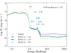
Figure 1: Different UVB models at $z$ ${\sim}$ 2.5 used in this study. The blue, black and green solid lines are used for KS18 UVB with $\alpha$ = $-1.6,-1.8$ and $-2.0$, respectively. The red dotted line shows the HM12 UVB. The vertical lines are used to show the ionization energy of different ions (ion name is marked right next to the line).

In our analysis, we use updated UVBs computed by KS18 and HM12 considering both quasars and galaxies as ionizing sources. In Fig. 1, we compare different UVB spectra at $z=2.5$. The quasar contribution to the integrated UVB intensity at high energies mainly depends on the assumed average SED of quasars which is used in the calculation of quasar emissivity. Quasar SEDs over the whole range of wavelength is usually approximated by a power law of $f_{\nu}\propto\nu^{\alpha}$ (Francis et al., 1991; Vanden Berk et al., 2001; Scott et al., 2004; Shull et al., 2012; Telfer et al., 2002). The reported values of power-law index ($\alpha$) varies from $-0.72$ to $-1.96$ (e.g see Table. 1 of Khaire, 2017). The power law index is observationally measured up to 2 Ryd (Stevans et al., 2014), which is then extrapolated to higher energies to obtain the complete spectrum. The HM12 UVB uses $\alpha$ = $-$1.57 consistent with Telfer et al. (2002). Khaire (2017) has recently shown that the UVB estimated using $\alpha$ = $-1.6$ to $-2.0$ also reproduces the He ii Ly$\alpha$ optical depth as a function of $z$ very well (see also, Gaikwad et al., 2018b, a). KS18 provides UVB for a range of $\alpha$ values, following their paper we use UVB with $\alpha=-1.8$ as our fiducial model. In addition, KS18 UVB uses the updated column density distribution of neutral hydrogen from Inoue et al. (2014) while calculating the IGM opacity to the UVB.

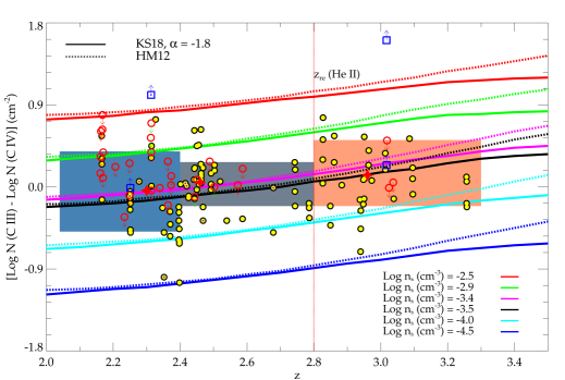
Figure 2: The observed ratio of $N$(C iii) to $N$(C iv) for 132 C iii components as a function of $z$ [104 clean detections (scattered yellow filled black circles), 24 components with upper limit on C iii (red open circles) and 4 components with lower limit on C iii (blue open squares)]. Predicted column density ratio of C iii to C iv for two different UVBs for model $M1$ are overplotted on top of the observed data. The solid and dashed lines are used to show the model predictions of KS18 and HM12 UVB, respectively. From top to bottom $n_{\rm\tiny H}$ is increasing as shown in the legends. The shaded blue, gray and orange regions show the range for redshift 2.1 < $z$ $\leq$ 2.4, 2.4 < $z$ $\leq$ 2.8 and 2.8 < $z$ $\leq$ 3.4 where 68% of observed data lies as obtained from the cumulative probability distribution of the sample data. The red filled stars are used to mark the median values of the column density ratios at each median redshift of the above three bins. The vertical red dotted line is used to mark the reionization redshift of He ii ($z_{re}$(He ii)) for our fiducial KS18 UVB model.

While these two UVBs (i.e our fiducial and HM12 UVBs) differ in spectral shape at low$-z$ ($z<1.0$) and high$-z$ ($z>3.5$), in the redshift range of our interest ($2.1<z<3.4$) the difference in H i photoionization rates ($\Gamma_{\rm HI}$) predicted by the two models is minimum (see Fig. 4 of KS18). However, our fiducial KS18 UVB spectrum shows different shape at E $>$ 4 Ryd and E $<$ 1 Ryd compared to that of HM12 because of the differences in the quasar emissivity and SED. At $z=2.5$ both UVBs provide $\Gamma_{\rm HI}$ consistent with the available measurements (Becker & Bolton, 2013; Bolton & Haehnelt, 2007) and the difference in $\Gamma_{\rm HI}$ between HM12 and KS18 is very small i.e ${\sim}$ $5\times 10^{-13}s^{-1}$.

The ionization energies of different ions are marked with vertical lines in Fig. 1. For the ions (for e.g. O ii, Si ii, Si iii, C ii and C iii) whose ionization energies are in the range E = 1 $-$ 4 Ryd, the UVB is contributed by the radiation coming from quasars as well as galaxies. However, for ions such as C iv the ionizing background radiation is dominated by quasars with no or negligible contributions from galaxies.

3.2 Modeling C iii absorbers

In photoionization models, ratio of column densities of two successive ionization stages of any element (for e.g. $\mbox{C\,{\sc iii}}/\mbox{C\,{\sc iv}}$, $\mbox{Si\,{\sc iii}}/\mbox{Si\,{\sc iv}}$, etc.) usually depends weakly on metallicity and depends mainly on the intensity and shape of the incident radiation field, density and temperature of the gas. Therefore, the basic idea of these models is to match the observed column density ratios of relative ions with the model predictions to determine $n_{\rm\tiny H}$ of the absorber for a given ionizing UVB. The metallicity of the gas is then adjusted to match the individual observed column densities of the heavy ions and $N({\mbox{H\,{\sc i}}})$. The specified initial conditions for each cloud are: (1) the UVB or ionizing continuum intensity and shape, (2) assumed $n_{\rm\tiny H}$ and the stopping criteria to terminate the calculation and (3) the chemical composition of the gas.

3.2.1 C iii absorbers as Jean’s stable clouds

In the first set of photoionization models (hereafter, $M1$ model), we assume the size of the cloud (or line-of-sight thickness) to be Jean’s length as suggested for the Ly$\alpha$ forest absorption by Schaye (2001). This is a reasonable approximation if C iii absorbers are predominantly originating from the IGM. Under this approximation the stopping total hydrogen column density ($N(H)$) in CLOUDY models for an assumed $n_{\rm\tiny H}$ (cm^-3) is given by (Schaye, 2001),

$$N(H)_{J}=n_{H}L_{J}\sim 1.6\times 10^{21}cm^{-2}{n_{H}}^{1/2}T_{4}^{1/2}\bigg{(}{\frac{f_{g}}{0.16}}\bigg{)}^{1/2}$$ (1)

where, $L_{J}$ is Jean’s length, $T_{4}(K)=T(K)/10^{4}$ and $f_{g}$ is the gas mass fraction. For the above calculations we use $T$ ${\sim}$$10^{4}$K, initial metallicity to be $10^{-2}$ Z_⊙ and $f_{g}$ $=$ 0.16 close to cosmic baryonic mass fraction. We varied $n_{H}$ (in a logarithmic scale) and redshift with step size of 0.1 to generate a grid of models and obtain the column densities for several ions of our interest.

In Fig. 2, we plot the observed ratio of $N({\mbox{C\,{\sc iii}}})$ to $N({\mbox{C\,{\sc iv}}})$ for 132 components [104 clean detections (yellow filled black circles), 24 components with upper limit on C iii (red open circles) and 4 components with lower limit on C iii (blue open squares)] in our sample as a function of $z$. We divide the entire redshift range into three bins, $[2.1,2.4]$ (blue shaded region), $[2.4,2.8]$ (gray shaded region) and $[2.8,3.4]$ (orange shaded region). In these redshift bins the measured column density ratio of C iii to C iv ranges (in logarithmic units) are $-0.49$ to $0.39$, $-0.21$ to $0.27$ and $-0.21$ to $0.52$, respectively where 68% of the observed data in each bin are distributed around the observed median.

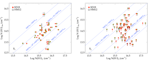
Figure 3: The observed neutral hydrogen column density, ${\rm log}$ $N$(H i), is plotted against the model $M1$ predicted neutral hydrogen column density ${\rm log}$ $N$(H i)_J for the two UVBs. Left-hand panel and right-hand panel show data from $S_{1}$ and $S_{2}$, respectively. Solid red circles and yellow filled squares show the results from KS18 and HM12 UVB, respectively. Black vertical line is used to represent error associated with the quantity where error is larger than the symbol size. The downward arrows represent the upper limits. The dashed blue lines represent different scaling of $N(\mbox{H\,{\sc i}})_{J}$ with $N(\mbox{H\,{\sc i}})_{obs}$. The text next to these line shows the linear scaling relation.

The red filled stars are used to mark the median values (-0.04, 0.05 and 0.13) of the observed column density ratios at each median values of redshift (2.30, 2.46 and 2.96) of the three redshift bins, respectively. We see a mild evolution in the median values of observed column density ratio with increasing redshift. As pointed out by KIM16, the apparent deficiency of C iii components at $z\sim 2.6$ is not real and caused by the lower number of quasar sightlines covered in this $z$ in the sample used.

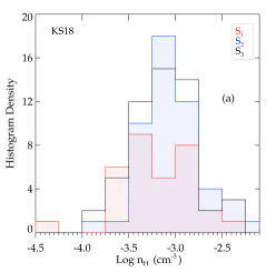
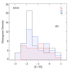
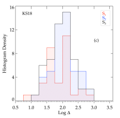
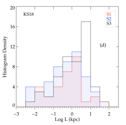
Figure 4: Histograms of derived parameters for model $M2$. Panel (a): hydrogen density ($n_{\rm\tiny H}$), panel (b): carbon abundances ($[C/H]$), panel (c): overdensity ($\Delta$) and panel (d): line-of-sight thickness, L of the components in logarithmic scale. Red, blue and black histograms are used to show the results for $S_{1}$, $S_{2}$ and $S_{3}$ data for our fiducial KS18 UVB, respectively.

Fig. 2 also shows the redshift evolution of column density ratio of C iii to C iv predicted by our models for two UVBs (Solid line for our fiducial KS18 UVB and dashed line for HM12 UVB). The model predictions show that this column density ratio increases mildly with increasing $z$ in the range 2 to 3.4 for a fixed hydrogen density of the absorber. Next, we use the observed $N({\mbox{C\,{\sc iii}}})/N({\mbox{C\,{\sc iv}}})$ to constrain $n_{\rm\tiny H}$ in the three redshift bins identified above. For the redshift bins [2.1, 2.4] and [2.8, 3.4], density range between $-$4.0 $<$ ${\rm log}$ $n_{\rm\tiny H}$ (in cm^-3) $<-2.9$ consistently reproduce the observed ratios (the blue and orange shaded regions) whereas for the mid redshift bin we require a density range from $-$3.6 $<$ ${\rm log}$ $n_{\rm\tiny H}$ (in cm^-3) $<$ $-$3.1 for the two UVBs. As discussed before this redshift range also shows slight deficit of systems. The overall range in density for all the absorber is $-$2.2 $<$ ${\rm log}$ $n_{\rm\tiny H}$ (in cm^-3) $<$ $-$4.5, for both the UVBs used in this analysis.

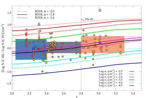
Figure 16: The observed ratio of $N$(C iii) to $N$(C iv) for 132 C iii components as a function of redshift [104 clean detections (scattered yellow filled black circles), 24 components with upper limit on C iii (red open circles) and 4 components with lower limit on C iii (blue open squares)]. $M1$ generated column density ratio of C iii to C iv for two different UVBs is over plotted on top of the observed data. The solid lines are used to show the model predictions using our fiducial KS18 with $\alpha$=-1.8. We also use KS18 UVB with $\alpha$ values -2.0 and -1.8 a shown by dotted and dash-dotted lines, respectability to compare the uncertainties in densities. From top to bottom $n_{\rm\tiny H}$ is increasing as shown in the legends. The shaded blue, gray and orange regions show the range for redshift 2.1 < $z$ $\leq$ 2.4, 2.4 < $z$ $\leq$ 2.8 and 2.8 < $z$ $\leq$ 3.4 where 68% of observed data lies as obtained from the cumulative probability distribution of the sample data. The red filled stars are used to mark the median values of the column density ratios at each median redshift of the above three bins. The vertical red dotted line is used to mark the reionization redshift of He ii ($z_{re}$(He ii)) for our fiducial KS18 UVB model.

The mild redshift evolution shown by the median values of observed column density ratio in the three redshift bins are well reproduced by the model with ${\rm log}$ $n_{\rm\tiny H}$ (in cm^-3) ${\sim}$ $-$3.4. It is also clear from Fig. 2 that model curves based on our fiducial KS18 UVB and that from HM12 differ from each other only at $z>2.5$. So the $n_{\rm\tiny H}$ required for models with HM12 UVB is slightly lower than that for our fiducial model in this redshift range. The observation as noted before in the text show larger range in quasar spectral index ($\alpha$) in the redshift of our interest (Khaire, 2017). So, we also consider two UVBs with quasar SEDs having $\alpha$ value $-1.6$ and $-2.0$. The results are shown in Fig. 16 (in the Appendix B). It is clear from Fig. 16 that a given $N$(C iii)/$N$(C iv) can be produced with lower $n_{\rm\tiny H}$ when we use UVBs generated using higher values of $\alpha$. It is also evident that an uncertainty in $\alpha$ of $\pm 0.2$ (with respect to our fiducial value $\alpha=-1.8$) translates to an uncertainty of $\pm$0.17 dex in the inferred $n_{\rm\tiny H}$ over the redshift range of interest in this study. This we will treat as a typical systematic uncertainty in the inferred $n_{\rm\tiny H}$ arising from allowed uncertainties in the quasar extreme-UV spectral index. It is also clear that the model predicted curves in $z$ $-$ $n_{\rm\tiny H}$ plane are parallel to each other so inferred redshift evolution of the derived parameters like $n_{\rm\tiny H}$ will not depend on our choice of $\alpha$ (unless otherwise there is a redshift evolution in $\alpha$).

As explained in Section. 2, not all C iii components shown in Fig. 2 have an aligned H i component which makes it difficult for us to constrain the physical conditions and chemical composition of such absorbers using photoionization models. However, detailed analysis is possible for the components in the sub-sample $S_{1}$ as these components have co-aligned H i component association. As our stopping criteria in the model $M1$ is the total hydrogen column density, the models predicted $N({\mbox{H\,{\sc i}}})$ (i.e., $N({\mbox{H\,{\sc i}}})_{J}$) can be compared with the observed $N({\mbox{H\,{\sc i}}})$ for these components denoted by $N({\mbox{H\,{\sc i}}})_{obs}$.

In Fig. 3 we compare $N({\mbox{H\,{\sc i}}})_{J}$ from both the models with the $N({\mbox{H\,{\sc i}}})_{obs}$. The result using our fiducial KS18 UVB and the HM12 UVB are plotted with solid red color circles and yellow filled squares, respectively. The dotted lines shows $N({\mbox{H\,{\sc i}}})_{obs}$ $\propto$ $N({\mbox{H\,{\sc i}}})_{J}$ for different proportionality constants (indicated above each line). It is clear from the figure that apart from one component the $N({\mbox{H\,{\sc i}}})_{obs}$ is systematically lower than the one predicted from our models. The observed $N({\mbox{H\,{\sc i}}})$ in the sample $S_{1}$ (left-hand panel of Fig. 3) shows a range, $N({\mbox{H\,{\sc i}}})$_obs${\sim}$ $7\times 10^{12}$ $-$ $1\times 10^{16}$ cm^-2 whereas, the model generated $N({\mbox{H\,{\sc i}}})$_J has a range from $2\times 10^{14}$ $-$ $1\times 10^{17}$ (in cm^-2) . The median value of the observed neutral hydrogen column density is, ${\rm log}$ $N({\mbox{H\,{\sc i}}})$ = 14.51 cm^-2 whereas our model generated median values of column densities are ${\rm log}$ $N({\mbox{H\,{\sc i}}})$ $=$ 16.04 cm^-2 and = 16.01 cm^-2 for HM12 and KS18 UVBs, respectively. Hence the median values of $N({\mbox{H\,{\sc i}}})$ predicted by model $M1$ is almost factor ${\sim}$ 32 higher than the observed column density for sample $S_{1}$ for the set of UVBs considered here. Moreover, there are ${\sim}$ 78% components in $S_{1}$ for which $N({\mbox{H\,{\sc i}}})_{J}$ is almost factor of 10 to 1000 or more times higher than $N({\mbox{H\,{\sc i}}})_{obs}$. This implies that if C iii components are in hydrostatic equilibrium then $f_{g}$ should be less than $1.6\times 10^{-3}$ in most of these components. Note the density range allowed in these clouds, even considering changes in $\alpha$, is not sufficient to alter this conclusion. Also most of the cases, assumed gas temperature is close to the inferred kinetic temperature from the Doppler parameter ($b$) values by KIM16.

In order to check whether this is the case for sample $S_{2}$ as well, we plot $N({\mbox{H\,{\sc i}}})$ predicted by our models with the observed $N({\mbox{H\,{\sc i}}})$ in the right-hand panel of Fig. 3. Here also we find median $N({\mbox{H\,{\sc i}}})_{J}$ is a factor of ${\sim}$24 higher than the median value of $N({\mbox{H\,{\sc i}}})$_obs with a similar trend as in sample $S_{1}$. Note that in this case the observed $N({\mbox{H\,{\sc i}}})$ could be an upper limit as H i absorption is not well aligned. However, the trend clearly supports that the conclusion derived for the sample $S_{1}$ may not be specific to the components with a well aligned H i absorption alone and may be more generic to the C iii components. This implies either $f_{g}$ is very small in these components or these C iii components are not in hydrostatic equilibrium with the dark matter or its self-gravity. In what follows we explore models with $N({\mbox{H\,{\sc i}}})$ as stopping criteria without imposing hydrostatic equilibrium condition given in Eq. 1.

3.2.2 Models with stopping criteria $N({\mbox{H\,{\sc i}}})$ $\approx$ $N({\mbox{H\,{\sc i}}})_{obs}$

As an alternative approach we construct another set of photoionization models (hereafter, model $M2$) where the observed value of $N({\mbox{H\,{\sc i}}})$ is used as the stopping criteria and the gas temperature is self-consistently calculated under photoionization equilibrium. Following similar approach as $M1$ we constrain $n_{H}$ for each component separately from the observed column density ratio of C iii to C iv. Once $n_{H}$ is constrained, we generate another grid of model outputs varying carbon abundances ($[C/H]$) in logarithmic scale of 0.1 to match with the individual observed column densities of C iii and C iv. This allows us to infer $n_{\rm\tiny H}$ and metallicity of the individual C iii components that have aligned C iv and H i absorption. We show histograms of different cloud properties obtained from $M2$ (which we quote as our fiducial model) in Fig. 4 for our fiducial KS18 UVB. In Table 4 we summarize the observed and model predicted column densities as well as the $n_{\rm\tiny H}$ and $[C/H]$ required by the models for $S_{1}$ components with clear detections.

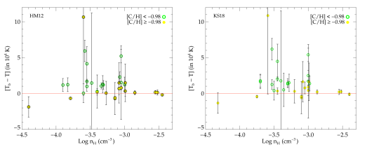
Figure 5: Difference in the temperature predicted by the photoionization model (T) for HM12 (left-hand panel) and our fiducial KS18 UVB (right-hand panel) and the inferred temperature (${\rm T_{b}}$) from the Voigt profile fitting. High metallicity (i.e $[C/H]>-0.98$) components are plotted in yellow color circles and the low metallicity components (i.e $[C/H]<-0.98$) are plotted with green open circles. The error bars show the 3$\sigma$ error range in $T_{b}$. It seems that $T_{b}-T$ deviations from zero occur at low metallicity and low density components.

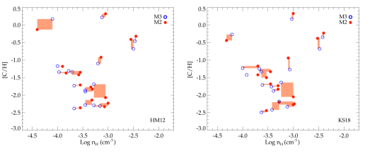
Figure 6: Comparison of hydrogen density and metallicity between two models $M2$ and $M3$for the 17 absorbers which are outside of $3\sigma$ range from $T_{b}$. for HM12 (left-hand panel) and KS18 (right-hand panel) UVBs. The red solid circles and blue open circles show the $M2$ and $M3$ outputs, respectively. The orange color patches are used to relate $M2$ to $M3$ values.

Hydrogen density: The hydrogen density range for the $32$ components in $S_{1}$ is, ${\rm log}$ $n_{\rm\tiny H}$ (in cm^-3) $\in$ [$-4.3$, $-2.4$], with a median ${\rm log}$ $n_{\rm\tiny H}$ (in cm^-3) of $-3.2$ for our fiducial KS18 UVB model. As expected this is similar to the $n_{\rm\tiny H}$ in model $M1$ that was required to fit median $N({\mbox{C\,{\sc iii}}})/N({\mbox{C\,{\sc iv}}})$ as a function of $z$. Left-hand top panel of Fig. 4 shows the histogram distribution of the hydrogen density derived in model $M2$ for all there samples. The required density distribution for the sub-sample $S_{2}$ and the sample $S_{3}$ are also shown in Fig. 4. The median ${\rm log}$ $n_{\rm\tiny H}$ (in cm^-3) $=$ $-$3.1 is found for both $S_{2}$ and $S_{3}$. As discussed before changing $\alpha$ between $-1.6$ and $-2.0$ introduces a systematic uncertainty in the inferred $n_{\rm\tiny H}$ by $\pm$0.17 dex. Assuming the uncertainty due to UVB in-addition to the slight offset due to allowed range in $n_{\rm\tiny H}$ to match the column densities, we notice that $n_{\rm\tiny H}$ distribution of well aligned components (sample $S_{1}$) is almost consistent with other two samples ($S_{2}$ and $S_{3}$). However, we note that the density we have obtained for individual components in $S_{1}$ are systematically higher by 1.2 to 1.3 dex compared to the values quoted by KIM16 (see their table A1 and A2) for the same components. As can be seen from figure 12 of KIM16, $\nu J_{\nu}$, values for HM12 shown are much lower than other UVB shown in that figure. In comparison to what we plot in Fig. 1, the HM12 UVB shown in KIM16 are off by a factor 1.1 dex. This could be accounted if KIM16 have missed a factor of 4$\pi$. If one uses the spectrum shown by KIM16 in the cloudy models then the derived density is expected to be smaller by at least one order of magnitude. We provide some details on this issue in Appendix A.

Carbon abundance: In panel (b) in Fig. 4, we show the $[C/H]$ distribution for the three samples. For $S_{1}$, the derived range for $[C/H]$ is [$-2.44$, $0.52$] with a median of $-0.98$. We find similar range of $[C/H]$ for other two samples irrespective of upper limits of column densities. However the median values of $[C/H]$ for $S_{2}$ and $S_{3}$ are $-1.27$ and $-1.64$, respectively which are moderately lower compared that of $S_{1}$. There are 4 components in $S_{1}$ and in total 8 components in the 53 absorption systems which show super solar metallicity. We find change in $\alpha$ between $-1.6$ and $-2.0$ leads to an uncertainty of 0.2 dex in the metallicity measurement based on our fiducial model. As can be seen from Table. 4, our metallicity measurements for most of the components in $S_{1}$ are slightly higher (i.e upto 0.4 dex with a median of 0.1 dex) than those derived by KIM16. This differences in density and metallicity motivate us to revisit different correlations found by KIM16 that were instrumental in drawing basic properties of the optically thin C iii components which we do in the following sections.

Overdensity ($\Delta$) and cloud thickness: In panel (c) of Fig. 4 we show the histogram distribution for overdensity ($\Delta$ = $n_{\rm\tiny H}$/<$n_{H}$> with <$n_{H}$> being the mean hydrogen density (<$n_{H}$> $=$ $1.719\times 10^{-7}$ cm^-3 $(1+z)^{3}$) of the uniform IGM that contains all the baryons). Simple analytic models of IGM Ly$\alpha$ forest at $z\sim 2.6$ suggests that most of the absorptions with ${\rm log}$ $N$(H i) $\leq$ 14 originate from regions with $\Delta\leq 4.0$ (i.e ${\rm log}$ $\Delta\leq-0.60$) (see Eq. 10 and Eq. 11 of Gaikwad et al., 2017a). The data shows a range of overdensities, ${\rm log}$ $\Delta$ $\approx$ $0.75-3.00$, with a median value, ${\rm log}$ $\Delta$ $=$ $2.0$ for all the components in our samples. As can be seen from Table 4, that most of the components in sample $S_{1}$ have ${\rm log}$ $N$(H i) $<$ 14.0. Our derived densities for these components clearly confirm that they are not like typical IGM clouds but they rather have higher densities and hence are more compact compared to the IGM clouds having similar $N$(H i). Since we have the information of $n_{\rm\tiny H}$ (in cm^-3) and $N$(H) (in cm^-2) for individual components we calculate the line-of-sight thickness defined as, L (in cm) = $N$(H)/$n_{\rm\tiny H}$. Fig. 4 panel (d) shows the histogram distribution of line-of-sight length, L in logarithmic scale. We find L for the 32 components in $S_{1}$ varying over a wide range from 7 pc to 35 kpc which is several times smaller than showed by KIM16 (20 kpc to 480 kpc). Similar range in L ($S_{2}$: 2 pc to 15 kpc, $S_{3}$: 8 pc to 35 kpc) is also seen for other two sub-samples where the line-of-sight thickness could be upper limits. Note that there are 3 components (component number 14, 15 and 30 in Table 4) with super-solar metallicity which have $L_{J}$ greater than 1000 times of $L$. We provide more detailed discussions on the possible origin for their line-of-sight thickness (or cloud size) in the following section.

Gas temperature: In the IGM (at say $z<5$), as the recombination time-scales are larger, the gas temperature at any epoch is decided by the energy injection by photoheating during the epoch of H i and He ii reionization followed by adiabatic cooling due to cosmological expansion (Hui & Gnedin, 1997). In the case of CGM, the temperature can be related to various local heating and cooling sources. However, the gas temperature (T) for our fiducial model is self-consistently calculated in CLOUDY under thermal equilibrium where recombination cooling is equated to the photoheating. Therefore, the temperature computed by CLOUDY need not be the correct kinetic temperature of the gas even when our estimated densities are much higher than the mean IGM density (<$n_{H}$>). In the case of sample $S_{1}$, KIM16 have obtained kinetic temperature (${\rm T_{b}}$) by decomposing the thermal and non-thermal contributions to the $b$ values. In Fig. 5, we plot the (${\rm T_{b}/T}$) as a function of $n_{\rm\tiny H}$ for HM12 and KS18 UVBs. High metallicity (i.e $[C/H]>-0.98$) components are plotted in yellow color circles and the low metallicity components (i.e $[C/H]<-0.98$) are plotted with green open circles. The error bar shows the 3$\sigma$ error range in $T_{b}$, where $\sigma$ is the error in $T_{b}$ obtained from the $b$ error. About ${\sim}$ 53 percent data points (component number 1, 5, 6, 7, 8, 9, 11, 12, 13, 15, 16, 17, 21, 23, 25, 27 and 28 in Table 4) in $S_{1}$  have temperature predicted by CLOUDY outside the range of $T_{b}\pm 3\sigma$ found by KIM16. It is clear from the Fig. 5 that points where $T$ is consistent with $T_{b}$ are the ones that also have high metallicity (i.e $[C/H]>-0.98$) and high density (${\rm log}$ $n_{\rm\tiny H}$ $\geq$ $-3.5$).

To quantify the effect of this discrepancy on the derived values of $n_{\rm\tiny H}$ and metallicity we setup another set of photoionization models (which we denote as $M3$). The basic CLOUDY modeling is same as $M2$, however we fix the gas temperature to be $T_{b}$ (i.e constant temperature models) given by KIM16 obtained from the $b$ value. In Fig. 6, we show the comparison of $n_{\rm\tiny H}$ and $[C/H]$ obtained from $M2$ and $M3$ for the 17 absorbers which are outside of $3\sigma$ range from $T_{b}$. The red and blue solid circles are used to denote the results for $M2$ and $M3$, respectively. The steel patches are used to show the differences between derived quantities from $M2$ and $M3$. The mean difference in density between $M2$ and $M3$ for the two UVBs are ($\Delta$ ${\rm log}$ ${n_{H}}$) = $0.1$ (resp. 0.12) and $(\Delta{[C/H]})=0.05$ (resp. 0.02) for our fiducial KS18 UVB (resp. HM12). Therefore, our models with only photoionization considerations do not introduce notable off-sets in the derived $n_{\rm\tiny H}$ and [C/H].

3.2.3 Model predictions for other ions

In order to verify the results of our fiducial model $M2$ we compare available observed column densities of several other ions (such as C ii, Si iii and Si iv) associated with the components with our model predictions. In Fig. 7, we show observed (or limiting) column density ratio of C ii to C iii with the predicted ratio from our model $M2$. Solid circles with error bars represent measurements. Note the quoted errors take into account the uncertainties in the model predictions due to UVB (as discussed earlier) and measurement uncertainties. The open circles with arrows are the upper limits. The black solid line represents the equality in both observed and model predicted column density ratio in logarithmic scale. The dotted lines give $\pm$0.13 dex uncertainty around this equality line. We show data for both components from sub-sample $S_{1}$ and $S_{2}$. Apart from four cases, C ii is not detected

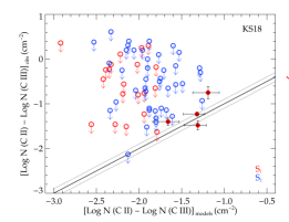
Figure 7: Comparison of observed column density ratio of C ii to C iii with the model predicted ratio for our fiducial KS18 UVB. Black horizontal bar is used to show error associated with the observed column density. Red and blue circles are used for $S_{1}$ and $S_{2}$, respectively. Filled circles are used to represent measurements and open symbols are used for upper limits on C ii column densities. The ‘y $=$ x’ equality is shown in black solid line. The black dotted lines show error range of $\pm$ 0.13 dex around this equality line due to the model uncertainties.

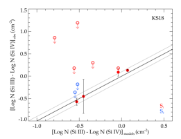
Figure 8: Comparison of observed column density ratio of Si iii to Si iv with the model predicted ratio for our fiducial KS18 UVB. Black vertical bars show the errors associated with the observed column densities. Red and blue circles are used for $S_{1}$ and $S_{2}$, respectively. Filled circles are used to represent measurements and open symbols are used for upper limits on Si iii column densities. The ‘y $=$ x’ equality line is shown in black solid line. The black dotted lines show error range of $\pm$ 0.13 dex around this equality line due to the model uncertainties.

in the C iii components. The derived upper limits on $N$(C ii)/$N$(C iii) for these components are consistent with our model predictions. In the four cases where we have the C ii absorption line detections our model predictions match with the observations within uncertainties.

For nine components in the sample $S_{1}$  (i.e component number 10, 13, 18, 19, 20, 23, 24, 29 and 30 in Table 4), we clearly detect Si iv. Four of these components (i.e 10, 18, 19 and 23 in Table 4) also show clear Si iii absorption. We obtained column densities of Si iv and Si iii by fitting Voigt profiles (with $b$ value consistent with the fits from KIM16) using VPFIT (Carswell & Webb, 2014). For Si iii non-detections we obtained upper limits assuming the $b$ value similar to C iii. There are two components in $S_{2}$ for which we could get upper limits on the ratio of Si iii to Si iv column densities. We show Voigt profile fit results for column densities and our fiducial model predicted results in Table C2 (see online supplementary data).

In Fig. 8, We show logarithm of observed column density ratio, ${\rm log}$ $N({\mbox{Si\,{\sc iii}}})/N({\mbox{Si\,{\sc iv}}})$ along with their predictions using model $M2$ for fiducial KS18 UVB. Black bars are used to show errors associated with the observed column density ratios. Red and blue color circles are used for samples $S_{1}$ and $S_{2}$, respectively. Filled circles are used to represent measurements and open symbols are used for components with upper limits on Si iii column densities and the black solid line shows equality in both the ratios and dotted lines give $\pm$0.13 dex uncertainty around this line. As can be seen from the figure the model predictions agree with the observed ratios within 0.1 dex for the four components that have clear detections. Also, all the upper limits are consistent with the model predictions. This confirms that the density constrains we obtained for the components based on the column density ratio of C iii to C iv are consistent with the observed Si iii to Si iv column density ratio. We next obtain the [Si/H] for each components by trying to reproduce the observed column density of Si iv. We find that [Si/C] $\sim 0.12\pm 0.10$ for these nine components. This once again confirms the consistency of metallicity we derived for individual components and [Si/C] in the C iii absorbers being close to solar value.

4 Redshift evolution of parameters

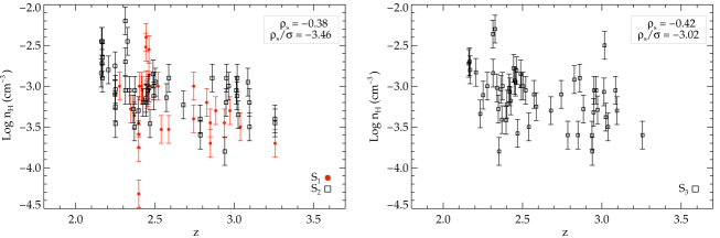
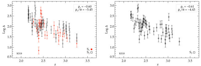
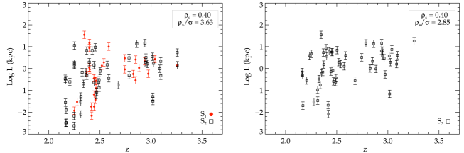
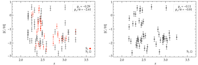
Figure 9: Redshift evolution of various parameter derived using our photoionization models (i.e model $M2$ using our fiducial KS18 UVB). The evolution of hydrogen density ($n_{\rm\tiny H}$), overdensity ($\Delta$), line-of-sight thickness (L) and metallicity (C/H) are plotted in different panels. In the left columns we plot the results for samples $S_{1}$ (red solid circles) and $S_{2}$ (open squares). The right columns show the results for $S_{3}$ where we have modeled the total column density for each system. In each panel we also show the rank correlation coefficient and its significance level.

In this section, we investigate the possible redshift evolution of derived parameters. In Fig. 9, we plot the redshift evolution of hydrogen density ($n_{\rm\tiny H}$), overdensity ($\Delta$), line-of-sight thickness (L) and metallicity ([C/H]) derived for our fiducial KS18 UVB and model $M2$. It is clear from the top-left-hand panel of this figure that the average density of the C iii components decreases with increasing $z$. Typical error bars shown take into account the uncertainty in our $n_{\rm\tiny H}$ measurements contributed by uncertainties in the UVB and in the column density measurements. For the components in the combined sample of $S_{1}$ and $S_{2}$ we find the Spearman rank correlation coefficient, $\rho_{s}=-0.38$ with a two-sided significance of its deviation from zero of $3\times 10^{-4}$ (or the anti-correlation is at 3.5$\sigma$ level). Combining $S_{1}$ and $S_{2}$ are justified as in all cases C iii and C iv are aligned. When we consider the average density in each C iii system (i.e sample $S_{3}$ shown in right-hand panels) the Spearman rank correlation coefficient is $\rho_{s}=-0.42$ and the two-sided significance of its deviation from zero is $2\times 10^{-3}$ (or the anti-correlation is at 3.0$\sigma$ level). Thus we find a statistically significant trend of increasing $n_{\rm\tiny H}$ associated with C iii absorbers with decreasing redshift.

In the second row from the top in Fig. 9, we show the gas overdensity $\Delta$ as a function of $z$. As expected this shows a much stronger anti-correlation with redshift. For components in the combined sample of $S_{1}$ and $S_{2}$ we find the Spearman rank correlation coefficient, $\rho_{s}=-0.60$ with a two-sided significance of its deviation from zero of $2\times 10^{-9}$ (or the anti-correlation is at 5.5$\sigma$ level). When we consider the average overdensity of each C iii system (i.e sample $S_{3}$ shown in right-hand panels) the Spearman rank correlation coefficient is $\rho_{s}=-0.61$ and the two-sided significance of its deviation from zero is $9\times 10^{-7}$ (or the anti-correlation is at 4.4$\sigma$ level). As discussed before, for the measured $N$(H i), the C iii absorbers tend to originate from gas having larger $\Delta$ compared to what one expects for a typical IGM gas. However, the inferred $n_{\rm\tiny H}$ is less than what is seen in the ISM of galaxies. Therefore, the optically thin C iii components studied here are most probably originating from gas outside the galactic discs (outflows, inflows or galactic halo gas). In summary, our results suggest that C iii absorbers tend to probe regions of higher density (and hence higher overdensity) as we move towards lower redshifts.

In the third row from the top in Fig. 9, we plot the line-of-sight thickness (L) as a function of $z$. For components in the combined sample of $S_{1}$ and $S_{2}$ we find the Spearman rank correlation coefficient, $\rho_{s}=0.40$ with a two-sided significance of its deviation from zero of $2\times 10^{-4}$ (or the correlation is at 3.6$\sigma$ level). When we consider the full system as a cloud (sample $S_{3}$), we have $\rho_{s}=0.40$ with a two-sided significance of its deviation from zero of $3\times 10^{-3}$ (or the correlation is at 2.9$\sigma$ level). Thus there is a statistically significant evidence for the low$-z$ (i.e $2.1\leq$z$\leq 2.5$) C iii absorbers being smaller in size compared to those at high$-z$ (i.e $z\geq 2.5$). However, unlike for $n_{\rm\tiny H}$ or $\Delta$ at low$-z$, in the case of L, we notice that the spread in L is very large and a population of sub-kilo-parsec components are predominantly present. Lack of such C iii components at the high$-z$ could drive the observed $z$ evolution of $L$. We discuss the origin of L in more details in the following section.

Table 1: Results of correlation analysis between different derived parameters and their $z$ dependence for sample $S_{1}$+$S_{2}$ 

	Full sample		For $z<2.5$		For $z\geq 2.5$
Parameters	$\rho_{s}$	$\rho_{s}/\sigma$	$\rho_{s}$	$\rho_{s}/\sigma$	$\rho_{s}$	$\rho_{s}/\sigma$
${[C/H]}$ versus ${\rm log}$ $L$	$-$0.68	$-$6.09	$-$0.66	$-$4.60	$-$0.62	$-$3.50
${\rm log}$ N(C iv) versus ${\rm log}$ $L$	+0.19	+1.69	+0.37	+2.60	+0.07	+0.38
${\rm log}$ N(H i) versus ${\rm log}$ $L$	+0.59	+5.26	+0.60	+4.30	+0.57	+3.21
${\rm log}$ N(C iv) versus ${[C/H]}$	+0.42	+3.76	+0.29	+2.00	+0.52	+2.94
${\rm log}$ N(H i) versus ${[C/H]}$	$-$0.65	$-$5.80	$-$0.64	$-$4.5	$-$0.59	$-$3.35

Table 2: Correlation analysis for sub-samples from $S_{1}$+$S_{2}$ based on L and [C/H]

	For ${[C/H]}$ $<$ -1.22		For ${[C/H]}$ $\geq$ -1.22		For ${\rm log}$ $L$ $<$ -1.0 kpc		For ${\rm log}$ $L$ $\geq$ -1.0 kpc
Parameters	$\rho_{s}$	$\rho_{s}/\sigma$	$\rho_{s}$	$\rho_{s}/\sigma$	$\rho_{s}$	$\rho_{s}/\sigma$	$\rho_{s}$	$\rho_{s}/\sigma$
${\rm log}$ N(C iv) versus ${\rm log}$ $L$	$+$0.50	$+$3.16	$+$0.54	$+$3.44	….	….	….	….
${\rm log}$ N(H i) versus ${\rm log}$ $L$	$+$0.41	$+$2.59	$+$0.51	$+$3.22	….	….	….	….
${\rm log}$ N(C iv) versus ${[C/H]}$	….	….	….	….	$+$0.59	$+$2.58	$+$0.65	$+$5.12
${\rm log}$ N(H i) versus ${[C/H]}$	….	….	….	….	$-$0.47	$-$2.03	$-$0.50	$-$3.91

In the bottom row of Fig. 9, we plot the [C/H] as a function of $z$. KIM16 have noticed a possible $z$ evolution of [C/H] (see their Fig. 22). When we consider individual components (true even for systems as a whole), the derived [C/H] of $z<2.5$ components shows a large spread compared to those at $z\geq 2.5$. In particular, we find components with [C/H] $\geq-1$ are rare at $z\geq 2.5$. This trend is very much similar to the trend we notice for L above. In the case of individual components this lack of high metallicity components at high$-z$ causes an anti-correlation with $\rho_{s}=-0.29$ having a two-sided significance of its deviation from zero of 0.008 (or the anti-correlation is at 2.6$\sigma$ level). While the trend is apparent for the sample $S_{3}$, we do not find any significant anti-correlation (i.e $\rho_{s}=-0.11$ with a significance level of 0.8$\sigma$). As suggested by KIM16 the lack of high metallicity points at the high$-z$ can not be attributed to the lack of sensitivity. A linear regression fit to the left-hand panel gives [C/H] = ($-0.84\pm 0.06$) $z$ + (1.01$\pm$0.16). This is a steeper evolution compared to the redshift evolution measured in DLAs by Rafelski et al. (2012) ($<Z>$ = $(-0.22\pm 0.03)$ $z-(0.65\pm 0.09)$, see their Fig. 11) upto $z$ $\approx$ 5.

In summary, we do find a strong evolution (i.e $>3\sigma$ level) in $n_{\rm\tiny H}$, $\Delta$ and L as a function of $z$. [C/H] shows a moderate (i.e 2.5$\sigma$ level) increase with decreasing $z$. It is quite possible that the the $z$ evolution of $L$ and [C/H] are driven by the appearance of compact clouds having high [C/H] only at $z<2.5$. We explore this aspect further in the following sections.

5 Correlations between derived parameters

KIM16 have found interesting correlations between different parameters derived for individual components. As our predicted parameters are different from earlier results (in particular $n_{\rm\tiny H}$ and $L$, mainly because we suspect KIM16 missed factor of 4$\pi$ in the UVB intensity, see Appendix A.), we investigate the correlations between different derived physical parameters in this section keeping in mind the redshift evolution discussed above. In Table 1, we summarize the Spearman rank correlation coefficient ($\rho_{s}$) and significance of $\rho_{s}$ in terms of $\sigma$ (i.e $\rho_{s}/\sigma$) for different combinations of parameters and redshift ranges. This table also provides the correlation statistics for low and high$-z$ sub-samples.

In the top panel of Fig. 10, we plot the $L$ vs. [C/H] for components in the combined sample of $S_{1}$ and $S_{2}$ in the left-hand panel and for $S_{3}$ in the right-hand panel, respectively. We indicate our derived $z$ scaling with symbol sizes (small size being smaller $z$ and vice-versa) and $n_{\rm\tiny H}$ in vertical color-bar as shown in Fig. 10. A clear anti-correlation between [C/H] and L (as found by KIM16) is evident in this figure. Spearman rank correlation analysis confirms an anti-correlation ($\rho_{s}=-0.68$) between these two quantities at 6.09$\sigma$ level. Despite our individual L values being smaller than that of KIM16 the anti-correlation found by them still remains valid. The anti-correlation still exists (albeit with slightly reduced significance level) even when we divide the sample in to two redshift bins. We find a strong anti-correlation with $\rho_{s}={-0.52}$ with a two-sided significance of its deviation from zero of $4.0\times 10^{-3}$ or the anti-correlation at 3.77$\sigma$ level is preset even for $S_{3}$. Note recently Muzahid et al. (2018) showed that line-of-sight thickness of high metallicity Si ii and C ii absorbers at low $z$ tend to be smaller compared to high $z$ ones. They use the integrated column density for those cases as in our sample $S_{3}$. The discussion presented here clearly confirms the existence of a correlation between metallicity and L among the C iii components. We discuss the possible origins for this correlation in the following section.

In the second row from the top in Fig. 10, we plot L versus $N$(H i). We use thick outer rim circles with color coding to represent individual [C/H] values with our above conventional symbol sizes for $z$ and same color schemes for $n_{\rm\tiny H}$ as stated above. We find a very strong correlation between these two quantities with $\rho_{s}=0.59$ with 5.26$\sigma$ significant level for the combined sample $S_{1}$+$S_{2}$. A strong correlation is also seen (albeit with reduced significance) when the sample is divided in to two redshift bins (see Table  1) or based on [C/H] (see Table 2). We also see the same trend for sample $S_{3}$ with $\rho_{s}=0.52$ at 3.73$\sigma$ significant level. Given the two correlations discussed till now we expect a strong anti-correlation between [C/H] and $N$(H i). This is what we find for [C/H] and $N$(H i) with $\rho_{s}=-0.65$ significant at 5.80$\sigma$ level for sample $S_{1}$+$S_{2}$ (see Table 1). However, the same is slightly lower with $\rho_{s}=-0.35$ significant at 2.50$\sigma$ level for sample $S_{3}$ due to the integrated column density.

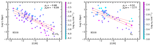
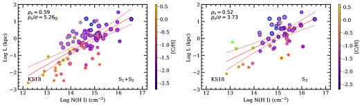
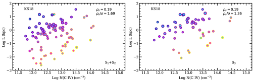
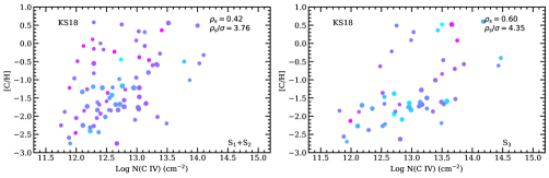
Figure 10: Correlation study of different parameters predicted by our fiducial photoionization model $M2$. In the left columns we plot the results for samples $S_{1}$+$S_{2}$ (solid circles). The right columns show the results for $S_{3}$. Top panels: the line-of-sight length L as a function of [C/H] , second panels: L as a function of $N({\mbox{H\,{\sc i}}})$, third panels: L as a function of $N({\mbox{C\,{\sc iv}}})$ and bottom panels: [C/H] as a function of $N({\mbox{C\,{\sc iv}}})$. In the top panels the vertical color-bar represents $n_{\rm\tiny H}$ in logarithmic unit. The solid circles sizes increase with increasing redshift. In the second panel the the vertical color-bar represents [C/H] values. We show same color codings (for $n_{\rm\tiny H}$ and [C/H]) and corresponding symbol sizes (for $z$) in the respective panels. In each panel we also show the rank correlation coefficient with significance level. The dashed solid line indicates linear regression fit to the data in upper two left-hand panels where we have found correlations significant at more than 5$\sigma$ level. The red dashed lines show the 1$\sigma$ range allowed by the regression analysis.

In the third row from the top in Fig. 10, we plot the observed C iv column density vs. the measured line-of-sight thickness ($L$) (this is similar to Fig. 18 of KIM16). For the full sample ($S_{1}$+$S_{2}$), we do not find any statistically significant correlation or anti-correlation between $N$(C iv) and L (see Table 1). We do not find any correlation (i.e more than 3$\sigma$ level) when we consider sub-samples in two different redshift bins. KIM16 based on their L versus $N({\mbox{C\,{\sc iv}}})$ plot suggested the existence of two population of C iii absorbers. In the case of large $L$ components, $L$ is found to be a weak function of $N({\mbox{C\,{\sc iv}}})$ whereas for L $\leq$ 20 kpc, $L$ increase rapidly with increasing $N({\mbox{C\,{\sc iv}}})$. However, we find a $\sim 3\sigma$ correlation when we divide the sample based on metallicity (see Table 2). Note that the sub-sample based on metallicity is identical to sub-sample based on L as there is a high anti-correlation between the two. Our study do not firmly support the trend found by KIM16 as contamination of high $[C/H]$ components to larger $L$ is evident from the figure. We also notice the same for sample $S_{3}$. Note that KIM16 have found apparent lack of points in the L versus $N({\mbox{C\,{\sc iv}}})$ plane with intermediate values of L when only $S_{1}$ is considered. They interpreted this as the existence of two different C iii  populations. However, in the combined sample the distribution becomes more uniform. While the L measurements of $S_{2}$ are limits (in the absence of perfectly aligned $N({\mbox{H\,{\sc i}}})$ measurements), the above formed demarcation could come from L versus [C/H] seen in the full sample. It will be important to increase the numbers of measurements to probe existence of this bimodal distribution at high statistical significance. In the following section, we address the lack or weak correlation between L and $N$(C iv) of the full sample when there is more than 5$\sigma$ correlation between $N$(H i) and L using simple photoionization considerations.

In the bottom panels of Fig. 10, we plot $N$(C iv) versus [C/H]. For any given $N$(C iv), we notice a large scatter in the measured [C/H]. However, there is a clear lack of low metallicity and high $N$(C iv) components. This leads to an apparent correlation between the two quantities. We find a correlation with $\rho_{s}=0.42$ significant at $\sim 3.76$ $\sigma$ level. It is evident from Table 1 that the correlation is slightly stronger for the high$-z$ sub-sample compared to the low$-z$ sub-sample. It is also interesting to note from Table 2 that the $N$(C iv) and [C/H] show a significant correlation (i.e 5.12$\sigma$ level) when we consider only components having $L$ greater than median L of our sample. The $N({\mbox{C\,{\sc iv}}})$ $-$ $[C/H]$ plane clearly does not show any distinct population as mentioned above. Furthermore, we see mild evolution in $N({\mbox{C\,{\sc iv}}})$ as a function of $[C/H]$ for the two metallicity ranges considered in the sub-samples contrary to the strong correlation reported earlier.

In summary, we find three combinations L versus [C/H], L versus $N$(H i) and $[C/H]$ versus $N$(H i) of parameters which show correlation or anti-correlation at more than 5$\sigma$ level. In the following section, using simple toy models, we try to understand these correlations and hence the origin of C iii absorbers.

6 Simple phenomenological models

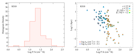
Figure 11: Left-hand panel: Histogram of pressure (i.e P/k) in individual components in $S_{1}$ and $S_{2}$. Right-hand panel: ($P/k$) versus $L$. It is clear that there is a tendency for the high metallicity components that also have slightly larger density to have higher pressure. Here we use different symbols and colors to show the distributions of the combined sample ($S_{1}$ + $S_{2}$) on basis of the median values. The red and blue circles represent high $n_{\rm\tiny H}$ ($n_{\rm\tiny H}$ $\geq$ $-3.1$), low $n_{\rm\tiny H}$ ($n_{\rm\tiny H}$ $<$ $-3.1$) components whereas the black and cyan open triangles show the high$-z$ (z $\geq$ 2.5) and low$-z$ (z $<$ 2.5) absorbers, respectively. Solid yellow and green circles represent high and low [C/H] components with respect to the median value $-1.2$, respectively.

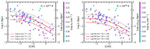
Figure 12: Left-hand panel: Comparison of observed length (L) vs. metallicity ([C/H]) relationship (color embedded circles for sample $S_{1}$ and $S_{2}$) with the simple isochoric cooling case. The vertical color-bar represents $n_{\rm\tiny H}$ in logarithmic unit. The solid circles sizes increase with increasing redshift. The continuous line shows the cooling length scale ($c_{s}t_{cool})$ with our median density $10^{-3.1}$ cm^-3, where $c_{s}$ is the sound speed at final temperature ($T_{f}$) = $10^{4.53}$ K (we use $\gamma$ = 1.3 for this calculation) and $t_{cool}$ is the cooling time scale starting from an initial temperature of $10^{5.2}K$. The dotted and dashed lines are used indicate the results for 1$\sigma$ range around this mean density (i.e ${\rm log}$ $n_{\rm\tiny H}$ = $-3.6$ and $-2.6$). Right-hand panel: Same as the left-hand panel but for isobaric case. The continuous line shows the cooling length scale ($c_{s}t_{cool})$ with our median pressure (${\rm log}$ $P/k$) = 1.39 cm^-3 K, where $c_{s}$ is the sound speed at final temperature ($T_{f}$) = $10^{4.53}$ K (we use $\gamma$ = 1.3 for this calculation) and $t_{cool}$ is the cooling time scale starting from an initial temperature of $10^{4.8}K$. The dotted and dashed lines are used for two different range of high-pressure and low-pressure (1$\sigma$ around median) which is, ${\rm log}$ $P/k$ (cm^-3 K) = 1.89 and 0.89, respectively.

One of the main results from the correlation analysis discussed in the previous section is the existence of a strong anti-correlation between [C/H] and line-of-sight thickness, $L$. All the discussions presented till now clearly suggest that the cloud sizes are not driven by hydrostatic equilibrium considerations (either with self-gravity or with the associated dark matter particles). Also the inferred over-densities of individual clouds are much higher than what is expected for gas in the IGM but less than what one expects in the interstellar medium of typical galaxies. Therefore, it is reasonable to assume that the C iii components are originating from the halos (or CGM) of galaxies.

First, we show the distribution of thermal pressure, $P/k$ in $cm^{-3}K$ (where $k$ is the Boltzmann’s constant) obtained from CLOUDY for individual components in left-hand panel of Fig. 11. We find the median ${\rm log}$ $P/k$ = $1.39\pm 0.5$ (1$\sigma$ range). In the models we consider below, we try to achieve the final gas pressure to this median value. In the right panel of Fig. 11, we plot ${\rm log}$ $P/k$ versus $L$. We also use different symbols to identify high and low density (also metallicity) components depending on our median values. It is clear from this figure that high metallicity components that are also smaller in size tend to have larger gas pressure compared to their low metallicity counterparts.

Metal enriched compact low temperature clouds in galactic halos can originate from winds that are ubiquitous in high$-z$ star forming galaxies (Veilleux et al., 2005). These winds could carry cold gas clouds from the multi-phased ISM (i.e the entrainment scenario), or clouds form in-situ in the CGM through thermal instabilities (Field, 1965; Meerson, 1989; Burkert & Lin, 2000) or condensation of cold gas clumps in-flows from hot halos (Hennebelle & Pérault, 1999; Sharma et al., 2012). Recently, McCourt et al. (2018) have argued that the fragmentation is an easier way to reach equilibrium and they considered this to be analogous to the Jeans instability in the gravitational collapse. They basically argued that ${L}\propto c_{s}t_{cool}$, where $c_{s}$ and $t_{cool}$ are the local sound speed and gas cooling time, respectively. They evaluated L at the temperature T where the product ${c_{s}t_{cool}}$ is minimized. To get the metallicity dependent on $L$, we need to evaluate this at a temperature T (or over the temperature range) where cooling rate depends strongly on the metallicity. In addition, in our case the gas of interest is also being heated and ionized continuously by the meta-galactic UVB radiation. Thus the final gas temperature we observe will be the photoionization equilibrium temperature of the gas. Without going into the detailed modelling and just to capture the basic picture, we consider a simple case where we calculated the “isochoric” and “isobaric” cooling time for a gas having initial temperature ($T_{i}$), [C/H] and $n_{\rm\tiny H}$ to reach the final temperature and pressure close to the median temperature and pressure that we infer for the C iii components. We use appropriate cooling curves for different metallicities as given in Schure et al. (2009).

In the “isochoric” case, we obtain the relationship between ${c_{s}t_{cool}}$ and [C/H] for different initial temperatures keeping the gas density to be constant at median density (i.e ${\rm log}$ $n_{\rm\tiny H}$ = $-$3.1). In the left hand panels of Fig. 12, we show the observed L versus [C/H] data overlayed with the isochoric model predictions of ${c_{s}t_{cool}}$ for three different $n_{\rm\tiny H}$ (i.e for the median and 1$\sigma$ range around it) obtained for Log T_i = 5.2. These curves clearly predict an anti-correlation between L and [C/H] as observed in our data. Note that the observed slope may be slightly steeper than the predictions of our constant density model but this could be accommodated if we allow the metallicity dependent density as hinted by the data in Fig. 11. For the assumed temperature range and density the cooling time-scale is found to be 2.5$\times 10^{6}$ years and 5.0$\times 10^{7}$ years, respectively for [C/H] = 0 and $-2$. These time-scales are much smaller than the typical free fall time-scale in the halos. Just to check whether the above mentioned anti-correlation is generic prediction of cooling based arguments we also consider the “isobaric” case (right-hand panel in Fig. 12)

In the “isobaric” case, for any assumed T_i we fix the initial density of the gas in such a way to maintain the pressure equal to the median observed $P/k$ $=1.39\pm 0.5$ ($1\sigma$ range). As the gas cools, we readjust the density to keep the pressure constant. If we start with the same initial temperature as we have for the “isochoric” case then the cooling time-scales are much longer as the gas starts with much lower density (as we try to keep the pressure constant) that leads to a longer cooling time-scale and larger cloud sizes. However, what is important to note here is that for a given choice of initial temperature (and final pressure) anti-correlation between L and [C/H] is clearly evident. As an illustration, we show models for three final $P/k$ and T_i = $8\times 10^{4}$ K. Here again allowing for the final pressure to be higher for the high metallicity gas compare to the low metallicity gas will make the curve more steep.

In summary, the toy models considered here provide the basic anti-correlation found between L and [C/H]. This lend supports to the idea that ${c_{s}t_{cool}}$ may be the main parameter deciding the physical extent of the C iii absorbers. We once again reiterate the fact that the calculations considered here are not rigorous enough to draw more quantitative conclusions. The main inference to carry forward is that for a given observed $n_{\rm\tiny H}$ the $L$ (or $N(H)$) depends on metallicity, perturbed density and temperature (i.e initial density and temperature) of the instability. Thus we expect a lack of strong correlation between $n_{\rm\tiny H}$ and $N(H)$ unlike in the case of hydrostatic equilibrium considerations. We shall keep this in mind while considering other correlations. To proceed further, we fit the observed correlation with a linear regression fit to obtain the following relationship,

$$log\leavevmode\nobreak\ {L}=(-1.26\pm 0.12)+(-0.78\pm 0.08){\rm{[C/H]}}.$$ (2)

The linear regression fit with a 1$\sigma$ range is shown in Fig. 10. We will use this to understand correlations related to C iv. In comparison, KIM16 have obtained line-of-sight thickness, ${\rm log}$ $L_{temp}$ = $-0.24$ $-$ 1.21 $\times$ ${[C/H]}$ with the $L_{temp}$ being at least one order of magnitude higher than our values for any given value of [C/H]. We provide linear regression fit to three significant correlation in Table 6, 7 and 8 which we found in the previous section for combined sample $S_{1}$+$S_{2}$ and individual sample $S_{2}$.

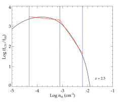
Figure 13: The ratio of fraction of C iv to fraction of H i as function of $n_{\rm\tiny H}$ at our median redshift value z $=$ 2.5. The vertical black dotted line is used to show our median density value (${\rm log}$ $n_{\rm\tiny H}$ (cm^-3) $=$ $-3.1$) and the blue lines show the boundary of ${\rm log}$ $n_{\rm\tiny H}$ ($-4.32$ and $-2.2$, resp) for sample S1+S2. The red dotted lines show linear fits to the plot for two $n_{\rm\tiny H}$ ranges, ${\rm log}$ $n_{\rm\tiny H}$ (cm^-3) $\in$ [$-3.1$, $-2.2$] and [$-4.32$, $-3.1$] with slope $-1.82$ and $-0.12$, respectively.

Next, we try to understand the implications of the strong correlation found between L and $N$(H i). For this we consider a constant density cloud in photoionization equilibrium. To start with we get an expression for L in terms of $N$(H i),

$${L} = {N_{\tiny H}\over n_{\tiny H}}={N(\mbox{H\,{\sc i}})\over f_{\tiny\mbox{H\,{\sc i}}}n_{\tiny H}}={N(\mbox{H\,{\sc i}})\leavevmode\nobreak\ \Gamma_{\tiny\mbox{H\,{\sc i}}}\over\alpha_{0}\leavevmode\nobreak\ n_{\tiny H}^{2}\leavevmode\nobreak\ T^{-0.78}}$$ (3)

$$\propto N(\mbox{H\,{\sc i}})\leavevmode\nobreak\ n_{\tiny H}^{-2}\leavevmode\nobreak\ T^{0.78}$$

$$\propto N(\mbox{H\,{\sc i}})\leavevmode\nobreak\ n_{\tiny H}^{0.78(\gamma-1)-2}.$$

Here, $\Gamma_{\tiny\mbox{H\,{\sc i}}}$ is the H i photoionization rate, $f_{\tiny\mbox{H\,{\sc i}}}$ the neutral hydrogen fraction and $\alpha_{\tiny 0}$ is the recombination coefficient which depends on the kinetic temperature as $T^{-0.78}$. For the last step we have assumed that the gas follows an equation of state (i.e $T\propto n^{\gamma-1}$). In the case of isothermal equation of state (i.e $\gamma=1$) we expect L $\propto N$(H i)$n_{\rm\tiny H}$^-2 and for $\gamma=5/3$ we expect L $\propto N$(H i)$n_{\rm\tiny H}$^-1.4. Therefore, any deviation from a linear relationship between L and $N$(H i) will be driven by the relationship between $N$(H i) and $n_{\rm\tiny H}$. Based on a linear regression fit we find L$\propto$ $N$(H i)^0.8±0.1 (see Fig. 10) which suggests that at best there is a very weak correlation between $n_{\rm\tiny H}$ and $N$(H i) (i.e $n_{\rm\tiny H}$$\propto$ $N$(H i)^0.10 or $N$(H i)^0.14 for the two equations of state discussed above). Note this lack of correlation is expected in the framework of models considered above. Our direct correlation analysis also confirms the lack of correlation found between $n_{\rm\tiny H}$ and $N$(H i) in our data (with a correlation coefficient of 0.2 having a significant level of 1.9$\sigma$).

The third strongest correlation we see is between $N$(H i) and [C/H]. Using Eq. 2 and 3 we can derive,

$$Log\leavevmode\nobreak\ N(\mbox{H\,{\sc i}})\propto(-0.98\pm 0.18){[C/H]}.$$ (4)

Thus the observed strong anti-correlation between $N$(H i) and [C/H] can also arise from simple considerations. Indeed the linear regression fit between $N$(H i) and [C/H] measurements is given by, $Log\leavevmode\nobreak\ N(\mbox{H\,{\sc i}})=(13.77\pm 0.11)-(0.62\pm 0.07){[C/H]}$ which is acceptable with the above expectations.

Lastly we try to understand the lack of correlation between $N$(C iv) and L. From simple considerations of Eq. 2 and 4, we can write the column density of C iv in terms of $N$(H i) as,

$$N(\mbox{C\,{\sc iv}}) = 10^{{[C/H]}}N(\mbox{H\,{\sc i}})(f_{\tiny\mbox{C\,{\sc iv}}}/f_{\tiny\mbox{H\,{\sc i}}})$$ (5)

$$\simeq L^{-0.025\pm 0.22}(f_{\tiny\mbox{C\,{\sc iv}}}/f_{\tiny\mbox{H\,{\sc i}}}).$$

Here, $f_{\tiny\mbox{C\,{\sc iv}}}$ is the ion fraction of C iv. Thus if the ratio of ion fraction of C iv to H i remains constant we expect only a weak correlation between $N$(C iv) and L. Presence of a strong correlation/anti-correlations between $L$ and $f_{\tiny\mbox{C\,{\sc iv}}}/f_{\tiny\mbox{H\,{\sc i}}}$ alone can set any possible correlation between $N({\mbox{C\,{\sc iv}}})$ and $L$. In Fig. 13, we show the ion fraction ratio as a function of density obtained from our fiducial model at the mean redshift of the data used here. At low density (${\rm log}$ $n_{\rm\tiny H}$ $<$ $-3.1$) it is clearly evident that $L$ has no/weak dependent on $N({\mbox{C\,{\sc iv}}})$ as $f_{\tiny\mbox{C\,{\sc iv}}}/f_{\tiny\mbox{H\,{\sc i}}}$ is nearly constant for the low $n_{\rm\tiny H}$ range. As expected we find $N(\mbox{C\,{\sc iv}})\propto L^{-0.01\pm 0.15}$ from the model predictions in these regions for the optically thin C iii components. However, at high $n_{\rm\tiny H}$ range (${\rm log}$ $n_{\rm\tiny H}$ $\geq$ $-3.1$) the ratio of ion fraction decreases monotonically with density i.e. $f_{\tiny\mbox{C\,{\sc iv}}}/f_{\tiny\mbox{H\,{\sc i}}}\propto$ $n_{\rm\tiny H}$^-1.83±0.02 as shown in the figure whereas we find $n_{\rm\tiny H}$ $\propto L^{-0.07\pm 0.03}$ with $\rho_{s}$ $=$ $-0.21$ at $-1.4\sigma$ confidence level for the $S_{1}$+$S_{2}$ components. This results in a mild correlation with $N(\mbox{C\,{\sc iv}})\propto L^{0.12\pm 0.04}$ for these high $n_{\rm\tiny H}$ components. Despite the lack of a correlation for overall components, we find 3$\sigma$ level correlation between these two with slope 0.96 and 0.73 for $logL=A+B$ ${\rm log}$ $N(\mbox{C\,{\sc iv}})$ for high and low metallicity branch, respectively (see Table 6). Within errors the slope is consistent with the slope of L versus $N({\mbox{H\,{\sc i}}})$. From Eq. 5, it is clear that when we restrict our samples to smaller metallicity ranges, L dependence on [C/H] is weak as compared to the higher metallicity sample.

7 Summary and discussions

We have presented detailed photoionization models for optically thin C iii absorption components in the redshift range $2.1<z<3.4$ along 19 quasar sightlines analyzed by KIM16. The main motivations for this re-analysis is to study the dependence of the assumed UVB on the derived parameters and thereby quantify systematic uncertainties in these parameters and understand various correlations between them.

We mainly focused on 53 absorption systems where C iii and C iv column densities are measured using Voigt profile fitting. Excluding the shifted or blended C iii components from these 53 systems, we consider two sub-samples $S_{1}$ and $S_{2}$ where Voigt profile fitting is performed using tied parameters for H i out of total 132 C iii components. The sub-sample $S_{1}$ consists of 32 intervening C iii components that also have a co-aligned H i component whereas $S_{2}$ consists of 50 intervening C iii components with moderately-aligned H i component or having upper limits on C iii. We also construct $S_{3}$ which includes all the 53 C iii systems where we consider the total column density of ions (i.e sum of the column density in individual Voigt profile components) to originate from single cloud in our models in order to account for the possible complex velocity and density field of the gas. We have analyzed these absorbers using photoionization models with CLOUDY for two UVBs, the HM12 and KS18). In case of KS18, we use different UVBs generated by varying spectral slope ($\alpha$) of extreme-UV quasar SEDs ($\alpha$ = $-1.6$, $-1.8$ and $-2.0$) where $\alpha$ = $-1.8$ is our fiducial model.

First, we considered that all the C iii absorbers originating from metal enriched optically thin IGM. In this case, we have used the cloud size to be the stopping criteria with its value being equal to Jeans length as suggested for the Ly$\alpha$ forest absorption by Schaye (2001). Our fiducial KS18 UVB models reproduced the observed range in $N({\mbox{C\,{\sc iii}}})$/$N({\mbox{C\,{\sc iv}}})$ for total hydrogen densities, $n_{\rm\tiny H}$ ${\sim}$ $6.3\times 10^{-3}-4.8\times 10^{-5}$ cm^-3. We see a mild evolution in the median observed column density ratio $N({\mbox{C\,{\sc iii}}})$/$N({\mbox{C\,{\sc iv}}})$ with increasing redshift. This is also captured by our models purely from the redshift evolution of KS18 UVB. However, $N({\mbox{H\,{\sc i}}})$ values predicted by these models are almost a factor ${\sim}$ 40 higher than the observed H i column density in sample $S_{1}$. The same is also seen in sample $S_{2}$ despite the fact that we are probably considering upper limits for these cases. This clearly suggests that the sizes of clouds are significantly smaller than what was given by hydrostatic equilibrium arguments generally used for the IGM clouds.

Next, we considered models where the stopping criteria is the observed $N$(H i). In this case, the derived hydrogen density ($n_{\rm\tiny H}$) for individual components ranges from $10^{-4.3}$ $-$ $10^{-2.2}$ cm^-3 with a median value of $10^{-3.1}$ cm^-3 for combined sub-sample $S_{1}$+$S_{2}$ whereas for sample $S_{3}$ we have $10^{-3.9}$ $-$ $10^{-2.3}$ cm^-3 with a median value of $10^{-3.1}$ cm^-3. [C/H] is found to be in the range $-2.75$ to 0.58, with a median value of $-1.2$ for $S_{1}$+$S_{2}$ whereas the same range is $-2.7$ to 0.6 with a median value of $-1.6$ for $S_{3}$. The gas temperature obtained in our photoionization models do not match with that obtained from the $b$ values for some components. For these components, we considered additional photoionization models where we fix the gas temperature to the one obtained from the $b$. We find that the difference in temperature makes negligible difference to the derived parameters with a median difference of $<$ $\Delta$ ${\rm log}$ ${n_{H}}>$ = $0.1$ and $<\Delta$[C/H]$>=0.05$ for our fiducial KS18 UVB.

Using a range of UVB generated for the assumed range in the UV spectral energy distribution of quasars we obtained a systematic uncertainty of $\pm 0.17$ dex for the derived $n_{\rm\tiny H}$ and $\pm 0.2$ dex for [C/H]. Note that the UVB calculated by KS18 is normalized by matching the H i photoionization rate ($\Gamma_{\mbox{H\,{\sc i}}}$) measurements from the Lyman-$\alpha$ forest observations (Bolton & Haehnelt, 2007; Becker & Bolton, 2013). Considering the uncertainties in the measurements of $\Gamma_{\mbox{H\,{\sc i}}}$ will further increase the systematic uncertainties in the $n_{\rm\tiny H}$ measurements. However this normalization uncertainties will have much less effect on the derived metallicities.

The $n_{\rm\tiny H}$ values measured in our study are typically one order of magnitude higher than what has been derived by KIM16 (see Appendix A for possible explanation). Because of this, KIM16 overestimated the line of sight thickness of the C iii absorbers. We find the line-of-sight thickness of the clouds to be in the range of 2 pc to 35 kpc with a median value of 0.63 kpc for the individual C iii components in $S_{1}$ and $S_{2}$ whereas the median value is slightly higher (1.6 kpc) for $S_{3}$ as we consider total integrated column densities along the line-of-sight. For the measured $N({\mbox{H\,{\sc i}}})$ the C iii absorbers originate from gas having larger $\Delta$ compared to what is expected in a typical IGM gas. However, the inferred $n_{\rm\tiny H}$ is less than the observed ISM of galaxies. Therefore, the optically thin C iii components studied here are most probably associated with gas outside the galactic discs (outflows, inflows or galactic halo gas). The derived sizes of the clouds are consistent with the C iii components originating from the CGM of high$-$z galaxies. However, to confirm the association of C iii clouds with the CGM, it is important to identify galaxies at close impact parameters. Bielby et al. (2013) have presented Lyman break galaxies around two of these quasar sightlines (HE0940$-$1050 and PKS 2126$-$158) of our sample. But there is no clear association found for the C iii absorbers. It will be important to have deep imaging and spectroscopic observations in these quasar fields to identify galaxies associated with the C iii absorbers studied here.

We find that there are three combinations (L versus [C/H], L versus $N({\mbox{H\,{\sc i}}})$ and [C/H] versus $N({\mbox{H\,{\sc i}}})$) of parameters that show correlation or anti-correlation at more than 5$\sigma$ level. Using the linear regression analysis we obtained relationship between L and [C/H] as well as between and L and $N({\mbox{H\,{\sc i}}})$. Based on simple photoionization considerations this will mean a very weak correlation between $N({\mbox{H\,{\sc i}}})$ and $n_{\rm\tiny H}$ [i.e $n_{\rm\tiny H}$$\propto$ $N({\mbox{H\,{\sc i}}})$^0.1]. We also show the expected relationship between $N({\mbox{H\,{\sc i}}})$ and [C/H] based on the above two relationships which is consistent with what is observed. While strong correlation is seen between L and $N({\mbox{H\,{\sc i}}})$, no such correlation is seen between L and C iv. This can also be easily understood in simple photoionization models.

Using simple toy models we suggest the basic idea that $c_{s}t_{cool}$ may be the main parameter deciding the physical size of the C iii absorbers. In particular the observed correlation between $L$ and [C/H] can be obtained with a narrow range in $n_{\rm\tiny H}$ while considering “isobaric” or “isochoric” cooling. This supports fragmentation which is an easier way to reach equilibrium and is considered analogous to the Jeans instability in the gravitational collapse (McCourt et al., 2018). These metal enriched clouds in galactic halos may originate from winds that are ubiquitous in high$-z$ star forming galaxies. If cold clouds formed in-situ at large distances then their frequency of occurrence may have some links to the star formation rate in the host galaxies. Therefore, it will be important to consider C iii absorbers over large redshift ranges and associate their evolution with the global star formation rate density found from high$-z$ galaxies. This we wish to pursue in the near future.

Still there remain few uncertainties before drawing strong conclusions which are as follows: (i) velocity coincidence based on which we consider single cloud photoionization models to produce $N({\mbox{C\,{\sc iii}}})/N({\mbox{C\,{\sc iv}}})$ ratio need not corresponds to spatial coincidence, (ii) given the velocity resolution, single absorption can come from a collection of multiple clouds and (iii) whether one can produce the observed frequency of occurrence of C iii absorbers consistently using the inferred cloud sizes. Another issue that needs to be addressed is the survivability of these clouds. To address these, we need self-consistent CGM models.

Acknowledgements: AM acknowledges the financial support by DST-INSPIRE fellowship program of Govt. of India. AM and ACP are thankful to IUCAA for providing free hospitality and travel grant during the visits. We thank Sowgat Muzahid for useful comments and suggestions. The authors also wish to thank the anonymous referee for providing valuable comments and suggestions for improving the manuscript.

Appendix A Understanding the possible cause of difference in $n_{\rm\tiny H}$ between our calculations and that of KIM16 

KIM16 mentioned that they have used the HM12 UVB in their CLOUDY models. However, when we use the HM12 UVB in our models, we find our $n_{\rm\tiny H}$ values are systematically higher by at least one order of magnitude than their reported values. In this work, we obtain the best fit $n_{\rm\tiny H}$ and [C/H] by constructing grids of $n_{\rm\tiny H}$ and [C/H] in CLOUDY models for each system while KIM16 used grids of ionization parameter and [C/H]. Thus, it is possible that some mistake may have occurred in KIM16 while $n_{\rm\tiny H}$ was obtained from the best fitted ionization parameter. Alternatively, the difference in the derived $n_{\rm\tiny H}$ for each component between this paper and that of KIM16 could also come from the HM12 UVB used by them in their CLOUDY models which is less by a normalization factor (approximately $4\pi$). In Fig. 14, we show the comparison of HM12 UVB and the same UVB with a factor of 4$\pi$ lower intensity at $z$ $\approx$ 2.4620. A cursory look at the Fig. 14 and the figure 12 of KIM16 reveals that HM12 UVB intensity lower by a factor 4$\pi$ gives a good representation of the UVB used by KIM16. To just check our conjuncture, we run photoionization models with the rescaled HM12 UVB by a factor of 4$\pi$ lower intensity and calculate the $n_{\rm\tiny H}$ for all the individual C iii components. We produce the results in Table. 3 and show a comparison plot in Fig. 15 along with our derived $n_{\rm\tiny H}$ from HM12 UVB (see Table 4). It can be seen from the Table. 3 and Fig. 15 that for 60% of the components, our model predicted $n_{\rm\tiny H}$ values using rescaled HM12 UVB match with that of KIM16 within $1\sigma$ errors. Also, the results are consistent with each other within $2\sigma$ errors in 80% of the cases. Even in the remaining cases, the values we derive for $n_{\rm\tiny H}$ are typically 0.2 dex higher than the values derived by KIM16. We also find our [C/H] estimates are within 0.1 dex to the values derived by KIM16. The small differences can come from various reasons, such as the different modelling procedure or providing UVB at nearest redshift where the original HM12 tables exist instead of interpolating to the exact redshift of absorbers. Nevertheless, this exercise suggests that KIM16 might have missed 4$\pi$ factor in the HM12 UVB somewhere in their calculations which gives rise to one order of magnitude difference in the $n_{\rm\tiny H}$ values.

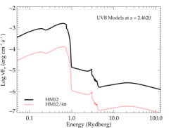
Figure 14: Comparison of HM12 UVB (black solid curve) with the one rescaled lower by a factor 4$\pi$ (red dotted curve) at $z$ $\approx$ 2.4620. Red dotted curve resembles the UVB shown by KIM16 in their figure 12.

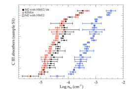
Figure 15: Comparison of $n_{\rm\tiny H}$ from different calculations. Black circles show our model $M2$ predicted $n_{\rm\tiny H}$ using rescaled HM12 UVB with a factor of 4$\pi$ lower intensity. Red diamonds show the calculations from KIM16 and blue squares show our model $M2$ derived $n_{\rm\tiny H}$ for HM12 UVB. The horizontal bars are errors associated with $n_{\rm\tiny H}$ in the respective calculations considering systematic uncertainties. Note that our derived $n_{\rm\tiny H}$ using HM12 UVB are consistently $\sim$1.1 dex higher than that inferred from rescaled HM12 UVB.

Table 3: Comparison of $n_{\rm\tiny H}$derived by KIM16 and by us using rescaled HM12 UVB.

#	quasar name	$z_{abs}$	log $n_{\rm\tiny H}$
			KIM16	This work
1	Q0055-269	3.257359	-5.01$\pm$0.05	-4.97$\pm$0.11
2	Q0055-269	3.038795	-4.87$\pm$0.10	-4.67$\pm$0.20
3	Q0055-269	2.744100	-4.39$\pm$0.08	-4.14$\pm$0.10
4	Q0055-269	2.743720	-4.81$\pm$0.18	-4.52$\pm$0.31
5	PKS2126-158	2.973015	-4.66$\pm$0.05	-4.38$\pm$0.08
6	Q0420-388	2.849598	-4.97$\pm$0.08	-4.86$\pm$0.12
7	Q0420-388	2.849229	-4.83$\pm$0.15	-4.62$\pm$0.24
8	HE0940-1050	2.937755	-4.8$\pm$0.05	-4.59$\pm$0.03
9	HE0940-1050	2.883509	-4.65$\pm$0.05	-4.37$\pm$0.08
10	HE0940-1050	2.826555	-4.54$\pm$0.05	-4.34$\pm$0.04
11	HE2347-4342	2.347467	-4.67$\pm$0.15	-4.38$\pm$0.27
12	HE0151-4326	2.519825	-4.45$\pm$0.08	-4.15$\pm$0.1
13	HE0151-4326	2.449902	-4.42$\pm$0.05	-4.22$\pm$0.05
14	HE0151-4326	2.419676	-4.41$\pm$0.05	-4.19$\pm$0.02
15	HE0151-4326	2.415718	-4.26$\pm$0.05	-4.16$\pm$0.01
16	HE0151-4326	2.401315	-4.41$\pm$0.15	-4.12$\pm$0.19
17	Q0002-422	2.539455	-4.85$\pm$0.05	-4.63$\pm$0.12
18	Q0002-422	2.463222	-4.2$\pm$0.05	-4.09$\pm$0.01
19	Q0002-422	2.462358	-3.53$\pm$0.05	-3.53$\pm$0.07
20	Q0002-422	2.462044	-3.74$\pm$0.10	-3.94$\pm$0.07
21	PKS0329-255	2.586757	-4.85$\pm$0.10	-4.63$\pm$0.23
22	PKS0329-255	2.456581	-4.4$\pm$0.30	-4.15$\pm$0.55
23	Q0453-423	2.444109	-3.34$\pm$0.10	-3.48$\pm$0.19
24	Q0453-423	2.442644	-3.67$\pm$0.05	-3.67$\pm$0.06
25	Q0453-423	2.441813	-4.41$\pm$0.20	-4.11$\pm$0.31
26	Q0453-423	2.398159	-5.37$\pm$0.10	-5.37$\pm$0.30
27	Q0453-423	2.397801	-4.91$\pm$0.05	-4.89$\pm$0.03
28	Q0453-423	2.397447	-4.86$\pm$0.08	-4.67$\pm$0.16
29	Q0453-423	2.396755	-4.57$\pm$0.05	-4.47$\pm$0.08
30	Q0453-423	2.277569	-4.12$\pm$0.05	-4.09$\pm$0.05
31	HE1347-2457	2.370003	-4.68$\pm$0.05	-4.46$\pm$0.07
32	Q0329-385	2.249389	-4.24$\pm$0.07	-4.24$\pm$0.40

Appendix B Redshift Evolution using KS18 UVB

Appendix C Predictions by CLOUDY photoionization models and correlation analysis tables of derived parameters

Table 4: $M2$ Cloudy-prediction column densities for the tied H i+C iv+C iii components of $S_{1}$ for the HM12 and KS18 UVBs.

Sl no.	quasar name	$z_{abs}$	Observed				Photoionization Model
			log $N({\mbox{H\,{\sc i}}})$	log $N(\mbox{C\,{\sc iv}})$	log $N(\mbox{C\,{\sc iii}})$	log $N(\mbox{C\,{\sc ii}})$	log $N(\mbox{C\,{\sc iv}})$		log $N(\mbox{C\,{\sc iii}})$		log $N(\mbox{C\,{\sc ii}})$		log $N(H)$
			in cm-2
							HM12	KS18	HM12	KS18	HM12	KS18	HM12	KS18
1	Q0055-269	3.25736	13.93$\pm$0.02	12.76$\pm$0.03	12.54$\pm$0.06	$\leq$12.3	12.76	12.76	12.54	12.56	9.98	10.17	18.24	17.93
2	Q0055-269	3.03880	14.60$\pm$0.04	12.72$\pm$0.04	12.59$\pm$0.15	$\leq$12.7	12.72	12.72	12.59	12.57	10.25	10.35	18.61	18.42
3	Q0055-269	2.74410	15.12$\pm$0.13	12.79$\pm$0.05	12.98$\pm$0.06	…	12.79	12.79	12.97	13	11.13	11.24	18.54	18.45
4	Q0055-269	2.74372	14.78$\pm$0.39	12.48$\pm$0.09	12.27$\pm$0.19	…	12.48	12.48	12.28	12.28	10.01	10.1	18.71	18.56
5	PKS2126-158	2.97302	14.36$\pm$0.01	12.18$\pm$0.03	12.25$\pm$0.03	$\leq$11.45	12.18	12.18	12.23	12.23	10.12	10.22	18.08	17.95
6	Q0420-388	2.84960	14.09$\pm$0.02	12.59$\pm$0.04	12.17$\pm$0.06	…	12.59	12.59	12.17	12.17	9.64	9.73	18.41	18.2
7	Q0420-388	2.84923	13.68$\pm$0.06	12.10$\pm$0.10	11.89$\pm$0.14	…	12.10	12.10	11.9	11.9	9.59	9.7	17.67	17.5
8	HE0940-1050	2.93776	14.58$\pm$0.02	12.65$\pm$0.02	12.51$\pm$0.01	$\leq$11.95	12.65	12.65	12.49	12.49	10.19	10.31	18.55	18.37
9	HE0940-1050	2.88351	14.60$\pm$0.01	12.35$\pm$0.03	12.37$\pm$0.02	$\leq$12.25	12.35	12.35	12.36	12.34	10.28	10.32	18.3	18.22
10	HE0940-1050	2.82656	14.51$\pm$0.21	13.19$\pm$0.02	13.23$\pm$0.03	$\leq$12	13.19	13.19	13.2	13.23	11.15	11.29	18.17	18.04
11	HE2347-4342	2.34747	15.99$\pm$0.20	13.49$\pm$0.00	13.26$\pm$0.22	$\leq$11.75	13.49	13.49	13.25	13.24	11.08	11.09	19.79	19.75
12	HE0151-4326	2.51983	15.24$\pm$0.02	12.29$\pm$0.04	12.35$\pm$0.06	$\leq$11.7	12.29	12.29	12.34	12.4	10.45	10.59	18.72	18.62
13	HE0151-4326	2.44990	14.45$\pm$0.02	12.99$\pm$0.01	12.96$\pm$0.04	$\leq$12.2	12.99	12.98	12.95	12.95	10.98	11.01	18.02	17.97
14	HE0151-4326	2.41968	12.85$\pm$0.04	12.75$\pm$0.01	12.76$\pm$0.02	…	12.75	12.75	12.75	12.78	10.87	10.92	16.31	16.28
15	HE0151-4326	2.41572	13.36$\pm$0.01	13.03$\pm$0.01	13.07$\pm$0.02	…	13.02	13.01	13.06	13.09	11.19	11.28	16.79	16.75
16	HE0151-4326	2.40132	15.04$\pm$0.02	12.34$\pm$0.11	12.37$\pm$0.06	…	12.34	12.34	12.37	12.41	10.49	10.58	18.51	18.45
17	Q0002-422	2.53946	14.24$\pm$0.03	12.55$\pm$0.02	12.18$\pm$0.06	$\leq$11.95	12.55	12.55	12.18	12.16	9.83	9.81	18.32	18.24
18	Q0002-422	2.46322	14.56$\pm$0.06	13.26$\pm$0.01	13.38$\pm$0.02	$\leq$11.75	13.26	13.26	13.36	13.38	11.55	11.59	17.95	17.93
19	Q0002-422	2.46236	15.16$\pm$0.02	13.20$\pm$0.01	13.83$\pm$0.03	12.60$\pm$0.03	13.20	13.20	13.85	13.85	12.54	12.53	18.02	18.04
20	Q0002-422	2.46204	14.83$\pm$0.02	13.34$\pm$0.02	13.59$\pm$0.02	12.19$\pm$0.08	13.34	13.34	13.59	13.6	11.93	11.94	18.06	18.06
21	PKS0329-255	2.58676	14.99$\pm$0.03	12.37$\pm$0.06	12.02$\pm$0.11	$\leq$11.9	12.37	12.37	12.03	12.01	9.7	9.68	19.03	18.96
22	PKS0329-255	2.45658	13.51$\pm$0.24	11.97$\pm$0.25	12.00$\pm$0.29	$\leq$12.3	11.97	11.97	12	12	10.09	10.11	17.01	16.98
23	Q0453-423	2.44411	14.62$\pm$0.01	12.63$\pm$0.06	13.41$\pm$0.08	12.66$\pm$0.11	12.63	12.64	13.36	13.42	12.12	12.23	17.4	17.35
24	Q0453-423	2.44264	14.91$\pm$0.01	13.04$\pm$0.03	13.66$\pm$0.07	12.18$\pm$0.07	13.04	13.04	13.65	13.66	12.3	12.35	17.8	17.78
25	Q0453-423	2.44181	14.67$\pm$0.01	11.75$\pm$0.13	11.83$\pm$0.14	$\leq$11.65	11.75	11.75	11.84	11.83	10.01	10.03	18.08	18.06
26	Q0453-423	2.39816	13.39$\pm$0.07	12.74$\pm$0.04	11.69$\pm$0.25	$\leq$12.05	12.74	12.74	11.71	11.71	8.87	8.79	18.45	18.34
27	Q0453-423	2.39780	14.41$\pm$0.01	13.78$\pm$0.01	13.16$\pm$0.02	$\leq$11.7	13.78	13.78	13.18	13.16	10.65	10.6	18.73	18.68
28	Q0453-423	2.39745	13.86$\pm$0.05	12.71$\pm$0.03	12.25$\pm$0.09	$\leq$11.8	12.71	12.71	12.27	12.23	9.9	9.81	17.97	17.95
29	Q0453-423	2.39676	14.16$\pm$0.03	13.34$\pm$0.01	13.06$\pm$0.04	$\leq$11.6	13.34	13.34	13.05	12.97	10.83	10.69	18.03	18.08
30	Q0453-423	2.27757	13.54$\pm$0.03	12.99$\pm$0.01	13.05$\pm$0.05	…	13.00	12.98	13.05	13.02	11.24	11.18	16.92	16.96
31	HE1347-2457	2.37000	14.10$\pm$0.09	12.60$\pm$0.03	12.33$\pm$0.04	$\leq$11.55	12.60	12.60	12.31	12.31	10.1	10.12	17.98	17.93
32	Q0329-385	2.24939	12.90$\pm$0.10	12.40$\pm$0.06	12.30$\pm$0.34	$\leq$12.55	12.41	12.40	12.3	12.3	10.33	10.33	16.45	16.46

Table 4	Continue…
Sl. no.	quasar name	$z_{abs}$	Photoionization Model
			log $n_{\rm\tiny H}$		$[C/H]$		log $\Delta$		log $L$		log $P/k$
			in cm-3						in kpc		in cm-3 K
			HM12	KS18	HM12	KS18	HM12	KS18	HM12	KS18	HM12	KS18
1	Q0055-269	3.25736	-3.90	-3.70	-1.18	-1.17	0.98	1.18	0.65	0.14	0.80	0.81
2	Q0055-269	3.03880	-3.60	-3.50	-1.7	-1.67	1.35	1.45	0.72	0.43	1.05	1.02
3	Q0055-269	2.74410	-3.05	-3.00	-1.63	-1.56	1.99	2.04	0.10	-0.04	1.49	1.44
4	Q0055-269	2.74372	-3.48	-3.40	-2.02	-2.02	1.56	1.64	0.70	0.47	1.17	1.14
5	PKS2126-158	2.97302	-3.34	-3.30	-1.77	-1.73	1.63	1.67	-0.07	-0.24	1.25	1.18
6	Q0420-388	2.84960	-3.83	-3.70	-1.37	-1.42	1.18	1.31	0.75	0.41	0.90	0.91
7	Q0420-388	2.84923	-3.55	-3.45	-1.35	-1.33	1.46	1.56	-0.27	-0.54	1.11	1.09
8	HE0940-1050	2.93776	-3.55	-3.45	-1.71	-1.68	1.43	1.53	0.61	0.33	1.10	1.07
9	HE0940-1050	2.88351	-3.31	-3.30	-1.83	-1.83	1.69	1.7	0.12	0.03	1.28	1.19
10	HE0940-1050	2.82656	-3.27	-3.20	-0.87	-0.8	1.75	1.82	-0.05	-0.25	1.31	1.28
11	HE2347-4342	2.34747	-3.32	-3.28	-2.14	-2.2	1.87	1.91	1.62	1.54	1.32	1.24
12	HE0151-4326	2.51983	-3.07	-3.00	-2.33	-2.27	2.05	2.12	0.30	0.13	1.50	1.46
13	HE0151-4326	2.44990	-3.14	-3.10	-0.92	-0.94	2.01	2.05	-0.33	-0.42	1.44	1.40
14	HE0151-4326	2.41968	-3.08	-3.05	0.53	0.52	2.08	2.11	-2.10	-2.16	1.43	1.40
15	HE0151-4326	2.41572	-3.05	-3.00	0.32	0.33	2.11	2.16	-1.65	-1.74	1.47	1.45
16	HE0151-4326	2.40132	-3.05	-3.00	-2.07	-2.05	2.12	2.17	0.07	-0.04	1.52	1.48
17	Q0002-422	2.53946	-3.58	-3.53	-1.42	-1.5	1.54	1.59	0.41	0.28	1.11	1.07
18	Q0002-422	2.46322	-2.99	-2.99	-0.59	-0.6	2.16	2.16	-0.55	-0.57	1.55	1.48
19	Q0002-422	2.46236	-2.52	-2.55	-0.43	-0.46	2.63	2.6	-0.95	-0.90	1.91	1.83
20	Q0002-422	2.46204	-2.85	-2.87	-0.58	-0.6	2.3	2.28	-0.58	-0.56	1.66	1.57
21	PKS0329-255	2.58676	-3.55	-3.53	-2.36	-2.44	1.55	1.57	1.09	1.00	1.13	1.05
22	PKS0329-255	2.45658	-3.08	-3.08	-0.93	-0.96	2.07	2.07	-1.40	-1.43	1.49	1.41
23	Q0453-423	2.44411	-2.45	-2.40	-0.32	-0.23	2.75	2.75	-1.64	-1.74	1.96	1.96
24	Q0453-423	2.44264	-2.55	-2.52	-0.41	-0.38	2.6	2.63	-1.14	-1.19	1.89	1.86
25	Q0453-423	2.44181	-3.00	-2.98	-2.23	-2.25	2.15	2.17	-0.41	-0.45	1.55	1.50
26	Q0453-423	2.39816	-4.40	-4.32	-0.13	-0.44	0.77	0.85	1.36	1.17	0.50	0.48
27	Q0453-423	2.39780	-3.79	-3.75	-0.36	-0.5	1.38	1.42	1.03	0.94	0.94	0.90
28	Q0453-423	2.39745	-3.60	-3.59	-0.86	-0.98	1.57	1.58	0.08	0.05	1.10	1.04
29	Q0453-423	2.39676	-3.40	-3.45	-0.46	-0.58	1.77	1.72	-0.06	0.04	1.24	1.13
30	Q0453-423	2.27757	-2.99	-3.00	0.17	0.08	2.23	2.22	-1.58	-1.53	1.53	1.47
31	HE1347-2457	2.37000	-3.40	-3.36	-1.14	-1.21	1.78	1.82	-0.11	-0.20	1.25	1.21
32	Q0329-385	2.24939	-3.14	-3.10	0.06	0	2.09	2.13	-1.90	-1.93	1.42	1.40

Table 5: $M2$ Cloudy-prediction for the tied Si iii and Si iv components of $S_{1}$ and $S_{2}$ for our fiducial KS18 UVB.

		Observed				Photoionization Models
#	$z_{abs}$	$logN(\mbox{Si\,{\sc iii}})$		$logN(\mbox{Si\,{\sc iv}})$		$logN(\mbox{Si\,{\sc iii}})$	$logN(\mbox{Si\,{\sc iv}})$	[C/H]	[Si/H]	Flag
			Error		Error
		(in cm-2)
Sample $S_{1}$
10	2.82656	11.45	0.08	12.02	0.02	11.49	12.02	-0.8	-0.69	Detection
13	2.4499	12.40	0.00	12.22	0.03	11.66	12.22	-0.94	-0.32	UL
18	2.46322	11.53	0.34	11.98	0.17	11.53	11.98	-0.6	-0.73	Detection
19	2.46236	12.73	0.07	12.64	0.05	12.60	12.64	-0.46	-0.46	Detection
20	2.46204	12.79	0.00	12.49	0.01	12.15	12.49	-0.6	-0.48	UL
23	2.44411	12.29	0.01	12.16	0.02	12.23	12.16	-0.23	-0.25	Detection
24	2.44264	12.81	0.00	12.63	0.01	12.59	12.63	-0.38	-0.21	UL
29	2.39676	12.38	0.00	11.52	0.07	10.73	11.52	-0.58	-0.43	UL
30	2.27756	12.92	0.00	11.73	0.11	11.21	11.73	0.08	0.09	UL
Sample $S_{2}$
1	2.45569	12.42	0.14	12.60	0.00	12.08	12.60	-2.02	-1.51	UL
2	2.25106	12.02	0.41	12.38	0.00	11.83	12.38	-0.55	-0.83	UL

Table 6: Linear regression fit coefficients for L as a function of $N({\mbox{C\,{\sc iv}}})$ and $N({\mbox{H\,{\sc i}}})$: log L = A + B log N(X) and associated Sphearman correlation coefficients.

Ion X	A	B	$\rho$	$\rho/\sigma$	Flag
		Sample $S_{1}$+$S_{2}$
C iv	-5.20$\pm$2.43	0.38$\pm$0.19	0.19	1.7	Full Sample
C iv	-13.32$\pm$2.84	0.96$\pm$0.22	0.54	3.44	For [C/H] $\geq$ -1.22
C iv	-8.99$\pm$2.34	0.73$\pm$0.19	0.5	3.16	For [C/H] $<$ -1.22
H i	-11.97$\pm$1.45	0.80$\pm$0.10	0.59	5.27	Full Sample
H i	-10.84$\pm$2.62	0.71$\pm$0.19	0.51	3.22	For [C/H] $\geq$ -1.22
H i	-7.35$\pm$1.97	0.50$\pm$0.13	0.41	2.59	For [C/H] $<$ -1.22
		Sample $S_{1}$
C iv	-3.65$\pm$4.62	0.26$\pm$0.36	-0.01	-0.01	Full Sample
C iv	-15.50$\pm$7.05	1.14$\pm$0.54	0.43	1.68	For [C/H] $\geq$ -0.98
C iv	-12.47$\pm$3.13	1.01$\pm$0.25	0.57	2.22	For [C/H] $<$ -0.98
H i	-9.95$\pm$2.94	0.67$\pm$0.20	0.30	1.65	Full Sample
H i	-6.56$\pm$4.91	0.41$\pm$0.35	0.26	1.02	For [C/H] $\geq$ -0.98
H i	-7.99$\pm$2.80	0.56$\pm$0.19	0.32	1.24	For [C/H] $<$ -0.98

Table 7: Linear regression fit coefficients for [C/H] as a function of $N({\mbox{C\,{\sc iv}}})$ and $N({\mbox{H\,{\sc i}}})$: log [C/H] = A + B log N(X) and associated Sphearman correlation coefficients.

Ion X	A	B	$\rho$	$\rho/\sigma$	Flag
		Sample $S_{1}$+$S_{2}$
C iv	-9.96$\pm$2.06	0.69$\pm$0.16	0.42	3.76	Full Sample
C iv	-2.55$\pm$1.93	0.16$\pm$0.15	0.15	0.94	For [C/H] $\geq$ -1.22
C iv	-5.42$\pm$1.81	0.28$\pm$0.15	0.37	2.32	For [C/H] $<$ -1.22
H i	9.66$\pm$1.31	-0.75$\pm$0.09	-0.65	-5.82	Full Sample
H i	4.50$\pm$1.54	-0.35$\pm$0.11	-0.45	-2.84	For [C/H] $\geq$ -1.22
H i	2.50$\pm$1.42	-0.29$\pm$0.09	-0.36	-2.3	For [C/H] $<$ -1.22
		Sample $S_{1}$
C iv	-11.24$\pm$3.63	0.80$\pm$0.29	0.52	2.90	Full Sample
C iv	0.10$\pm$3.64	-0.04$\pm$0.28	-0.11	-0.42	For [C/H] $\geq$ -0.98
C iv	-3.80$\pm$3.47	0.16$\pm$0.28	0.36	1.40	For [C/H] $<$ -0.98
H i	9.41$\pm$2.31	-0.73$\pm$0.16	-0.56	-3.13	Full Sample
H i	4.09$\pm$1.99	-0.32$\pm$0.14	-0.35	-1.35	For [C/H] $\geq$ -0.98
H i	6.00$\pm$1.74	-0.53$\pm$0.12	-0.81	-3.13	For [C/H] $<$ -0.98

Table 8: Linear regression fit coefficients for L as a function of [C/H]: log L = A + B [C/H] and associated Sphearman correlation coefficients.

A	B	$\rho$	$\rho/\sigma$	Flag
		Sample $S_{1}$+$S_{2}$
-1.27$\pm$0.12	-0.78$\pm$0.09	-0.68	-6.09	Full Sample
-1.32$\pm$0.16	-1.02$\pm$0.23	-0.61	-3.83	For [C/H] $\geq$ -1.22
-1.27$\pm$0.39	-0.76$\pm$0.20	-0.43	-2.72	For [C/H] $<$ -1.22
		Sample $S_{1}$
-1.13$\pm$0.21	-0.78$\pm$0.15	-0.62	-3.46	Full Sample
-1.30$\pm$0.29	-1.31$\pm$0.48	-0.64	-2.49	For [C/H] $\geq$ -0.98
-0.75$\pm$0.58	-0.54$\pm$0.32	-0.26	-0.99	For [C/H] $<$ -0.98

References

- Bechtold et al. (1994) Bechtold J., Crotts A. P. S., Duncan R. C., Fang Y., 1994, ApJ, 437, L83
- Becker & Bolton (2013) Becker G. D., Bolton J. S., 2013, MNRAS, 436, 1023
- Bielby et al. (2013) Bielby R., et al., 2013, MNRAS, 430, 425
- Bolton & Haehnelt (2007) Bolton J. S., Haehnelt M. G., 2007, MNRAS, 382, 325
- Burkert & Lin (2000) Burkert A., Lin D. N. C., 2000, ApJ, 537, 270
- Carswell & Webb (2014) Carswell R. F., Webb J. K., 2014, VPFIT: Voigt profile fitting program, Astrophysics Source Code Library (ascl:1408.015)
- Dedikov & Shchekinov (2004) Dedikov S. Y., Shchekinov Y. A., 2004, Astronomy Reports, 48, 9
- Dinshaw et al. (1997) Dinshaw N., Weymann R. J., Impey C. D., Foltz C. B., Morris S. L., Ake T., 1997, ApJ, 491, 45
- Faucher-Giguère et al. (2009) Faucher-Giguère C.-A., Lidz A., Zaldarriaga M., Hernquist L., 2009, ApJ, 703, 1416
- Fechner (2011) Fechner C., 2011, A&A, 532, A62
- Ferland et al. (2013) Ferland G. J., et al., 2013, Rev. Mexicana Astron. Astrofis., 49, 137
- Field (1965) Field G. B., 1965, ApJ, 142, 531
- Francis et al. (1991) Francis P. J., Hewett P. C., Foltz C. B., Chaffee F. H., Weymann R. J., Morris S. L., 1991, ApJ, 373, 465
- Gaikwad et al. (2017a) Gaikwad P., Choudhury T. R., Srianand R., Khaire V., 2017a, preprint, (arXiv:1705.05374)
- Gaikwad et al. (2017b) Gaikwad P., Srianand R., Choudhury T. R., Khaire V., 2017b, MNRAS, 467, 3172
- Gaikwad et al. (2018a) Gaikwad P., Srianand R., Khaire V., Choudhury T. R., 2018a, arXiv e-prints,
- Gaikwad et al. (2018b) Gaikwad P., Choudhury T. R., Srianand R., Khaire V., 2018b, MNRAS, 474, 2233
- Grevesse et al. (2010) Grevesse N., Asplund M., Sauval A. J., Scott P., 2010, Astrophysics and Space Science, 328, 179
- Gronke & Oh (2018) Gronke M., Oh S. P., 2018, MNRAS, 480, L111
- Haardt & Madau (1996) Haardt F., Madau P., 1996, ApJ, 461, 20
- Haardt & Madau (2012) Haardt F., Madau P., 2012, ApJ, 746, 125
- Heckman et al. (2017) Heckman T., Borthakur S., Wild V., Schiminovich D., Bordoloi R., 2017, ApJ, 846, 151
- Hennebelle & Pérault (1999) Hennebelle P., Pérault M., 1999, A&A, 351, 309
- Hui & Gnedin (1997) Hui L., Gnedin N. Y., 1997, MNRAS, 292, 27
- Hussain et al. (2017) Hussain T., Khaire V., Srianand R., Muzahid S., Pathak A., 2017, MNRAS, 466, 3133
- Ikeuchi (1986) Ikeuchi S., 1986, Ap&SS, 118, 509
- Inoue et al. (2014) Inoue A. K., Shimizu I., Iwata I., Tanaka M., 2014, MNRAS, 442, 1805
- Khaire (2017) Khaire V., 2017, preprint, (arXiv:1702.03937)
- Khaire & Srianand (2013) Khaire V., Srianand R., 2013, MNRAS, 431, L53
- Khaire & Srianand (2015a) Khaire V., Srianand R., 2015a, MNRAS, 451, L30
- Khaire & Srianand (2015b) Khaire V., Srianand R., 2015b, ApJ, 805, 33
- Khaire & Srianand (2018) Khaire V., Srianand R., 2018, preprint, (arXiv:1801.09693)
- Khaire et al. (2016) Khaire V., Srianand R., Choudhury T. R., Gaikwad P., 2016, MNRAS, 457, 4051
- Kim et al. (2016) Kim T.-S., Carswell R. F., Ranquist D., 2016, MNRAS, 456, 3509
- Liang & Remming (2018) Liang C. J., Remming I. S., 2018, preprint, (arXiv:1806.10688)
- McCourt et al. (2015) McCourt M., O’Leary R. M., Madigan A.-M., Quataert E., 2015, MNRAS, 449, 2
- McCourt et al. (2018) McCourt M., Oh S. P., O’Leary R., Madigan A.-M., 2018, MNRAS, 473, 5407
- Meerson (1989) Meerson B., 1989, ApJ, 347, 1012
- Miralda-Escude & Ostriker (1990) Miralda-Escude J., Ostriker J. P., 1990, ApJ, 350, 1
- Muzahid et al. (2018) Muzahid S., Fonseca G., Roberts A., Rosenwasser B., Richter P., Narayanan A., Churchill C., Charlton J., 2018, MNRAS, 476, 4965
- Pachat et al. (2016) Pachat S., Narayanan A., Muzahid S., Khaire V., Srianand R., Wakker B. P., Savage B. D., 2016, MNRAS, 458, 733
- Pachat et al. (2017) Pachat S., Narayanan A., Khaire V., Savage B. D., Muzahid S., Wakker B. P., 2017, MNRAS, 471, 792
- Planck Collaboration et al. (2016) Planck Collaboration et al., 2016, A&A, 594, A13
- Rafelski et al. (2012) Rafelski M., Wolfe A. M., Prochaska J. X., Neeleman M., Mendez A. J., 2012, ApJ, 755, 89
- Rees (1986) Rees M. J., 1986, MNRAS, 218, 25P
- Sargent et al. (1980) Sargent W. L. W., Young P. J., Boksenberg A., Tytler D., 1980, ApJS, 42, 41
- Schaye (2001) Schaye J., 2001, ApJ, 559, 507
- Schaye et al. (2007) Schaye J., Carswell R. F., Kim T.-S., 2007, MNRAS, 379, 1169
- Schure et al. (2009) Schure K. M., Kosenko D., Kaastra J. S., Keppens R., Vink J., 2009, A&A, 508, 751
- Scott et al. (2004) Scott J. E., Kriss G. A., Brotherton M., Green R. F., Hutchings J., Shull J. M., Zheng W., 2004, ApJ, 615, 135
- Shapiro et al. (1994) Shapiro P. R., Giroux M. L., Babul A., 1994, ApJ, 427, 25
- Sharma et al. (2012) Sharma P., McCourt M., Quataert E., Parrish I. J., 2012, MNRAS, 420, 3174
- Shull et al. (1999) Shull J. M., Roberts D., Giroux M. L., Penton S. V., Fardal M. A., 1999, AJ, 118, 1450
- Shull et al. (2012) Shull J. M., Stevans M., Danforth C. W., 2012, ApJ, 752, 162
- Smette et al. (1992) Smette A., Surdej J., Shaver P. A., Foltz C. B., Chaffee F. H., Weymann R. J., Williams R. E., Magain P., 1992, ApJ, 389, 39
- Sparre et al. (2018) Sparre M., Pfrommer C., Vogelsberger M., 2018, preprint, (arXiv:1807.07971)
- Stevans et al. (2014) Stevans M. L., Shull J. M., Danforth C. W., Tilton E. M., 2014, ApJ, 794, 75
- Telfer et al. (2002) Telfer R. C., Zheng W., Kriss G. A., Davidsen A. F., 2002, ApJ, 565, 773
- Thompson et al. (2016) Thompson T. A., Quataert E., Zhang D., Weinberg D. H., 2016, MNRAS, 455, 1830
- Vanden Berk et al. (2001) Vanden Berk D. E., et al., 2001, AJ, 122, 549
- Veilleux et al. (2005) Veilleux S., Cecil G., Bland-Hawthorn J., 2005, ARA&A, 43, 769
- Williger & Babul (1992) Williger G. M., Babul A., 1992, ApJ, 399, 385
- van de Voort et al. (2018) van de Voort F., Springel V., Mandelker N., van den Bosch F. C., Pakmor R., 2018, preprint, (arXiv:1808.04369)