Absence of Coulomb Blockade in the
Anderson Impurity Model
at the Symmetric Point

Abstract

In this work, we investigate the characteristics of the electric current in the so-called symmetric Anderson impurity model. We study the nonequilibrium model using two complementary approximate methods, the perturbative quantum master equation approach to the reduced density matrix, and a self-consistent equation of motion approach to the nonequilibrium Green’s function. We find that at a particular symmetry point, an interacting Anderson impurity model recovers the same steady-state current as an equivalent non-interacting model, akin a two-band resonant level model. We show this in the Coulomb blockade regime for both high and low temperatures, where either the approximate master equation approach and the Green’s function method provide accurate results for the current. We conclude that the steady-state current in the symmetric Anderson model at this regime does not encode characteristics of a many-body interacting system.

The Raymond and Beverly Sackler Center for Computational Molecular and Materials Science, Tel Aviv University, Tel Aviv, Israel 69978 Both authors contributed equally to this work Both authors contributed equally to this work Kavli Energy NanoScience Institute, Berkeley, California 94720, United States Materials Sciences Division, Lawrence Berkeley National Laboratory, Berkeley, California 94720, United States Materials Sciences Division, Lawrence Berkeley National Laboratory, Berkeley, California 94720, United States The Raymond and Beverly Sackler Center for Computational Molecular and Materials Science, Tel Aviv University, Tel Aviv, Israel 69978

1 Introduction

The Anderson impurity model ¹ is a fundamental model for studying strongly correlated open quantum systems that appears in many physical situations, including coupled quantum dots in semiconductor heterostructures ^{2, 3} and in molecular- and nano-electronics.^{4, 5} It is one of the simplest models of interacting particles and exhibits complex many-body phenomena, such as the Coulomb blockade,⁶ pair tunneling,⁷ and the Kondo effect.^{8, 9} Such nonequilibrium steady-state effects of interacting open quantum systems, continue to present a grand challenge for theory. As such, the Anderson impurity model is often used as a benchmark for developing approximate methods to study many-body physics of interacting particles, in and out of equilibrium.

In recent years, numerous approximate methods have been developed to study transport through nanoscale interacting systems. Among these are quantum master equation approaches and their generalizations,^{10, 11, 12, 13, 14, 15, 16} approaches based on the nonequilibrium Green’s function formalism,^{17, 18, 19, 20, 21, 22, 23, 24} and quasi-classical mapping techniques.^{25, 26} More recently, numerically exact approaches (namely, methods that allow for a systematic convergence of the results) have been proposed that allow for an assessment of the approximate methods in certain regimes of interactions and temperatures. Most notable are real-time path integral methods based on diagrammatic expansions of the hybridization or onsite interactions,^{27, 28, 29, 30, 31, 32, 33, 34, 35} renormalization group techniques,^{36, 37, 38} or many-body wavefunction techniques.³⁹ Benchmarks of the various approximation schemes are often limited to the so-called symmetric Anderson model,^{30, 25, 40, 41, 42} where the empty and fully occupied states of the impurity are degenerate.

In this work, we show that the steady-state current in the Anderson impurity model at the symmetric point coincides exactly with an equivalent noninteracting model, transition. The results presented in this study are derived from two complementary approximate methods: 1) the quantum master equation (QME) approach and 2) the equation of motion (EOM) nonequilibrium Green’s function (NEGF) approach.^{43, 44} The QME approach is adequate in the weak system-leads coupling limit and at high temperatures, for arbitrary onsite interactions, whereas the EOM-NEGF approach used here is accurate for small onsite interactions, but is not limited to weak system-bath couplings. These methods do not account for the Kondo effect or pair-tunneling. As such, this work focuses on the many-body physics of the Anderson model, which is manifested in the Coulomb blockade regime.

2 Model and methods

The Anderson impurity model is defined by the Hamiltonian $H=H_{S}+H_{B}+V$, where

$$H_{S}= \underset{\sigma=\uparrow,\downarrow}{\sum}\varepsilon_{\sigma}d_{\sigma}^{\dagger}d_{\sigma}+Ud_{\uparrow}^{\dagger}d_{\uparrow}d_{\downarrow}^{\dagger}d_{\downarrow}$$ (1)

describes the impurity (or dot), referred to simply as the ‘system Hamiltonian’,

$$H_{B}= \underset{\underset{k\in\rm L,\rm R}{\sigma=\uparrow,\downarrow}}{\sum}\varepsilon_{k}c_{k\sigma}^{\dagger}c_{k\sigma}$$ (2)

describes the noninteracting fermionic baths (or leads), and

$$V= \underset{\underset{k\in\rm L,\rm R}{\sigma=\uparrow,\downarrow}}{\sum}t_{k}d_{\sigma}^{\dagger}c_{k\sigma}+{\rm h.c.},$$ (3)

describes the hybridization between the system and the leads. In the above, $d_{\sigma}^{\dagger}\ \left(d_{\sigma}\right)$ are the creation (annihilation) operators of an electron on the dot with spin $\sigma=\uparrow,\downarrow$ with one-body energy of $\varepsilon_{\sigma}$, $U$ is the onsite Hubbard interaction, $c_{k\sigma}^{\dagger}\ \left(c_{k\sigma}\right)$ are the creation (annihilation) operators of an electron in mode $k$ of the leads with energy $\varepsilon_{k}$, and $t_{k}$ is the hybridization between the dot and mode $k$ in the lead. The coupling to the quasi-continuous leads is modeled by the leads’ spectral function, $\Gamma_{\ell}\left(\omega\right)$, where $t_{k\in\ell}=\sqrt{\Gamma_{\ell}\left(\varepsilon_{k}\right)\Delta\omega/2\pi}$ is the coupling between the dot and the $k$-th mode of the $\ell=\rm L,R$ bath, and $\Delta\omega$ is the discretization of the leads energy spectrum. Throughout, we take Planck’s constant to be 1, and assume that the coupling to the leads is spin-independent. When a wide-band limit is assumed, $\Gamma_{\ell}\left(\omega\right)=\Gamma_{\ell}$ is taken to be independent of $\omega$.

We will focus on two regimes of the model, the non-interacting regime where $U=0$ and $\varepsilon_{\uparrow}=\varepsilon_{\downarrow}=\varepsilon$, and the symmetric point where $\varepsilon_{\uparrow}=\varepsilon_{\downarrow}=-U/2$. The system is held out of equilibrium by an electric bias by setting the leads’ chemical potentials to be $\mu_{\ell}=\varepsilon_{f}+V_{\ell}$, where $\varepsilon_{f}$ is the Fermi energy of the leads and $V_{\ell}$ is the bias on the $\ell$th lead. A symmetric bias is said to be applied when $\varepsilon_{f}=0$. The many-body energy levels in both regimes of the system Hamiltonian, $H_{S}$, are schematically introduced in Fig. 1. An empty dot, $\left|0\right>$ with energy $0$, a singly-occupied dot with an electron in either spin, $\left|\sigma\right>=d^{\dagger}_{\sigma}\left|0\right>$ with energy $\varepsilon$, and a doubly occupied (or full) dot $\left|f\right>=d^{\dagger}_{\uparrow}d^{\dagger}_{\downarrow}\left|0\right>$, with energy $2\varepsilon+U$. We may note that in both cases studied all one-body transitions are given by the same energy difference, which is equal to $\varepsilon$. This is a key feature of the symmetric Anderson model, giving rise to identical one-body transition probabilities as the noninteracting case.

Figure 1: Schematic representation of the many-body energy levels of the system Hamiltonian, $H_{S}$. In red: the non-interacting system $U=0$, in black: the symmetric model $U=-2\varepsilon$. The Fermi energy of the leads, $\varepsilon_{f}$, around which the chemical potentials are biased, is set to zero.

We analyze the model using two methods, a quantum master equation approach and a nonequilibrium Green’s function approach. Although NEGF is typically more general and has a wider regime of validity than the QME approach, we present both results, as the perturbative QME approach facilitates a simple derivation. In the supporting material we discuss the validity of the approximations in more detail and compare the two methods in their appropriate regimes.

2.1 Quantum master equation

The quantum master equation description ^{45, 46} assumes weak-coupling between the dot and the leads, and is derived using second order perturbation theory in the dot-lead coupling strength. The time scale at which correlations in the leads decay should be smaller than the time scale for the leads to induce a significant change in the dot. This implies that the QME is valid when the temperature of the leads is sufficiently high with respect to the coupling strength (see supporting information for details). It is further assumed that there are no initial correlations between the dot and the leads, and that the leads are in local thermal equilibrium. Since the system Hamiltonian is diagonal in the many-body basis and the dot-lead coupling is bi-linear, the populations are coupled directly and not through the coherences. In other words, the equations of motion for the populations (diagonal terms of the reduced density matrix) and the coherences (non-diagonal terms) are decoupled in the many-body basis. Thus, if the initial state of the system is diagonal in the dot-energy eigen-basis or if we are interested in physical quantities that depend on populations alone, then the QME is reduced to a rate equation for the many-body states:

$$\left(\begin{array}[]{c}\dot{p}_{0}\\ \dot{p}_{\uparrow}\\ \dot{p}_{\downarrow}\\ \dot{p}_{f}\end{array}\right)=M\left(\begin{array}[]{c}p_{0}\\ p_{\uparrow}\\ p_{\downarrow}\\ p_{f}\end{array}\right),$$ (4)

Here $p_{0}$ is the probability of occupying the empty dot state $\left|0\right>$ , $p_{\uparrow}$ and $p_{\downarrow}$ are the probabilities of occupying the states $\left|\uparrow\right>$ and $\left|\downarrow\right>$ respectively, and $p_{f}$ is the probability of having a fully occupied dot corresponding to the state $\left|f\right>$. The transition matrix is given by

$$M=\sum_{\ell=\rm L,R}\left(\begin{array}[]{cccc}-\left(\gamma^{\ell}_{\uparrow 0}+\gamma^{\ell}_{\downarrow 0}\right)&\gamma^{\ell}_{0\uparrow}&\gamma^{\ell}_{0\downarrow}&0\\ \gamma^{\ell}_{\uparrow 0}&-\left(\gamma^{\ell}_{0\uparrow}+\gamma^{\ell}_{f\uparrow}\right)&0&\gamma^{\ell}_{\uparrow f}\\ \gamma^{\ell}_{\downarrow 0}&0&-\left(\gamma^{\ell}_{0\downarrow}+\gamma^{\ell}_{f\downarrow}\right)&\gamma_{\downarrow f}\\ 0&\gamma^{\ell}_{f\uparrow}&\gamma^{\ell}_{f\downarrow}&-\left(\gamma^{\ell}_{\uparrow f}+\gamma^{\ell}_{\downarrow f}\right)\end{array}\right),$$ (5)

where $\gamma^{\ell}_{ij}$ is the transition rate from state $j$ to state $i$ induced by the collective $\ell$ bath. The above rates can be calculated using Fermi’s golden-rule and satisfy local detailed balance such that $\gamma^{\ell}_{ij}=\gamma^{\ell}_{ji}\exp[\beta_{\ell}(\varepsilon_{j}-\varepsilon_{i})]$ where $\beta_{\ell}$ is the inverse temperature of the $\ell$-th lead and $\varepsilon_{i}$ is the energy of the eigenstate $i$.

Assuming symmetry between spin up and spin down, $\varepsilon_{\uparrow}=\varepsilon_{\downarrow}\equiv\varepsilon$, in the wide-band approximation, we can explicitly write

$$\gamma^{\ell}_{\uparrow 0} = \gamma^{\ell}_{\downarrow 0}\equiv\Gamma_{\ell}f^{\ell}(\varepsilon-\mu_{\ell})$$ (6)

$$\gamma^{\ell}_{0\uparrow} = \gamma^{\ell}_{0\downarrow}\equiv\Gamma_{\ell}f^{\ell}(-\varepsilon+\mu_{\ell})$$

$$\gamma^{\ell}_{f\uparrow} = \gamma^{\ell}_{f\downarrow}\equiv\Gamma_{\ell}f^{\ell}(\varepsilon+U-\mu_{\ell})$$

$$\gamma^{\ell}_{\uparrow f} = \gamma^{\ell}_{\downarrow f}\equiv\Gamma_{\ell}f^{\ell}(-\varepsilon-U+\mu_{\ell}),$$

where $f^{\ell}(\varepsilon-\mu_{\ell})=\left(1+\exp[\beta_{\ell}(\varepsilon-\mu_{\ell})]\right)^{-1}$ is the Fermi-distribution with the chemical potential $\mu_{\ell}$. We note that the results presented in the manuscript are not limited to a wide-band approximation and are valid for any even spectral function, $\Gamma_{\ell}(\varepsilon)=\Gamma_{\ell}(-\varepsilon)$.

The current from the $\ell$ bath is calculated according to

$$I_{\ell}(t)=\frac{e}{2}\sum_{ij}\left(N_{i}-N_{j}\right)J_{ij}^{\ell}\quad\text{where}\quad J_{ij}^{\ell}=\gamma_{ij}^{\ell}p_{j}(t)-\gamma_{ji}^{\ell}p_{i}(t),$$ (7)

where $N_{i}$ is the number of electrons in state $i$, and $J_{ij}^{\ell}$ is the probability current from state $j$ to state $i$, due to the coupling to the $\ell$ bath, and $e$ is the charge of the electron.

2.2 Equation of motion nonequilibrium Green’s functions

To support our findings we further investigate the Anderson model at the symmetric point using an EOM approach to NEGF.^{47, 21, 48, 49, 50} We note that the approach taken here is valid to all orders of $\Gamma$ but is exact to order $\Gamma^{2}U$. Thus, in the limit $U\rightarrow 0$ the NEGF approach recovers the exact noninteracting results for any system-bath coupling strength. The approach does not capture the Kondo and pair-tunneling effects but is capable of describing the Coulomb blockade regime.^{47, 21, 48, 49, 50} We begin by defining the impurity one-body nonequilibrium contour ordered Green’s function,^{43, 44, 51}

$$G_{\sigma}\left(\tau,\tau^{\prime}\right)=-i\left\langle\hat{T}_{c}\left[d_{\sigma}\left(\tau\right)d_{\sigma}^{\dagger}\left(\tau^{\prime}\right)\right]\right\rangle$$ (8)

where $\hat{T}_{c}$ is the contour ordering operator and the average $\langle\cdots\rangle$ should be interpreted as the trace over the many particle Hilbert space with the equilibrium density matrix at $t=-\infty$. The equation of motion for the Green’s functions on the Keldysh contour is obtained from the Heisenberg equation for the time propagation of the operators, leading to an equation of motion which introduces new, higher-order Green’s functions, for which equations of motion are also derived. For interacting Hamiltonians, this method produces a hierarchy of inter-dependent equations for Green’s functions of higher orders. A common procedure is to truncate the equations by choosing an appropriate approximation (or closure), after which the equations are solved self-consistently. In this work we use a closure that is exact for the noninteracting limit, where $U=0$, for any value of the system-leads coupling $\Gamma$, and at any temperature, reproducing the exact resonant level model solution. It also provides a good approximation at sufficiently large values of $U$, in the Coulomb blockade regime.^{47, 22} A detailed derivation of the closure is provided in the Supplementary Information.

We solve the equations of motion on the Keldysh contour and analytically continued to the real time axis using Langreth rules.⁵² The integral equations for the retarded and lesser NEGFs in steady state are transformed to the frequency domain, resulting in the following algebraic equations:

$$G_{\sigma}^{r}\left(\omega\right)= g_{\sigma}^{\left(0\right)r}\left(\omega\right)+g_{\sigma}^{\left(0\right)r}\left(\omega\right)\Sigma_{\sigma}^{r}\left(\omega\right)G_{\sigma}^{r}\left(\omega\right)+Ug_{\sigma}^{\left(0\right)r}\left(\omega\right)G_{\sigma}^{\left(2\right)r}\left(\omega\right),$$ (9)

$$G_{\sigma}^{\left(2\right)r}\left(\omega\right)= g_{\sigma}^{\left(U\right)r}\left(\omega\right)\left\langle n_{\bar{\sigma}}\right\rangle+g_{\sigma}^{\left(U\right)r}\left(\omega\right)\Sigma_{\sigma}^{r}\left(\omega\right)G_{\sigma}^{\left(2\right)r}\left(\omega\right),$$

$$G_{\sigma}^{<}\left(\omega\right)= g_{\sigma}^{\left(0\right)<}\left(\omega\right)+g_{\sigma}^{\left(0\right)r}\left(\omega\right)\Sigma_{\sigma}^{r}\left(\omega\right)G_{\sigma}^{<}\left(\omega\right)+g_{\sigma}^{\left(0\right)r}\left(\omega\right)\Sigma_{\sigma}^{<}\left(\omega\right)G_{\sigma}^{a}\left(\omega\right)$$

$$+ g_{\sigma}^{\left(0\right)<}\left(\omega\right)\Sigma_{\sigma}^{a}\left(\omega\right)G_{\sigma}^{a}\left(\omega\right)+Ug_{\sigma}^{\left(0\right)r}\left(\omega\right)G_{\sigma}^{\left(2\right)<}\left(\omega\right)+Ug_{\sigma}^{\left(0\right)<}\left(\omega\right)G_{\sigma}^{\left(2\right)a}\left(\omega\right),$$

$$G_{\sigma}^{\left(2\right)<}\left(\omega\right)= g_{\sigma}^{\left(U\right)<}\left(\omega\right)\left\langle n_{\bar{\sigma}}\right\rangle+g_{\sigma}^{\left(U\right)r}\left(\omega\right)\Sigma_{\sigma}^{r}\left(\omega\right)G_{\sigma}^{\left(2\right)<}\left(\omega\right)$$

$$+ g_{\sigma}^{\left(U\right)r}\left(\omega\right)\Sigma_{\sigma}^{<}\left(\omega\right)G_{\sigma}^{\left(2\right)a}\left(\omega\right)+g_{\sigma}^{\left(U\right)<}\left(\omega\right)\Sigma_{\sigma}^{a}\left(\omega\right)G_{\sigma}^{\left(2\right)a}\left(\omega\right),$$

where $\bar{\sigma}$ is the opposite spin to $\sigma$,

$$G_{\sigma}^{r}\left(t,t^{\prime}\right) =-i\theta\left(t-t^{\prime}\right)\left\langle\left\{d_{\sigma}\left(t\right),d_{\sigma}^{\dagger}\left(t^{\prime}\right)\right\}\right\rangle,$$ (10)

$$G_{\sigma}^{<}\left(t,t^{\prime}\right) =i\left\langle d_{\sigma}^{\dagger}\left(t^{\prime}\right)d_{\sigma}\left(t\right)\right\rangle,$$

$$G_{\sigma}^{\left(2\right)r}\left(t,t^{\prime}\right) =-i\theta\left(t-t^{\prime}\right)\left\langle\left\{d_{\sigma}\left(t\right)n_{\bar{\sigma}}\left(t\right),d_{\sigma}^{\dagger}\left(t^{\prime}\right)\right\}\right\rangle,$$

$$G_{\sigma}^{\left(2\right)<}\left(t,t^{\prime}\right) =i\left\langle d_{\sigma}^{\dagger}\left(t^{\prime}\right)d_{\sigma}\left(t\right)n_{\bar{\sigma}}\left(t\right)\right\rangle,$$

and $G\left(\omega\right)=\int_{-\infty}^{\infty}d\tau\,G\left(\tau\right)e^{i\omega\tau}$, with $\tau=t-t^{\prime}$. In the above, the steady state population of spin $\sigma$ is given by

$$\left\langle n_{\sigma}\right\rangle=\int_{-\infty}^{\infty}\frac{d\omega}{2\pi}G_{\sigma}^{<}\left(\omega\right),$$ (11)

and we used the following definitions for the noninteracting Green’s functions:

$$g_{\sigma}^{\left(\delta\right)r}\left(\omega\right) =\frac{1}{\omega-\varepsilon_{\sigma}-\delta+i\eta},$$ (12)

$$g_{\sigma}^{\left(\delta\right)<}\left(\omega\right) =2\pi\left\langle d^{\dagger}d\right\rangle_{0}\delta\left(\omega-\varepsilon_{\sigma}-\delta\right),$$

with $\delta=0$ or $\delta=U$. The self energy due to the coupling to the leads are given by:⁵³

$$\Sigma_{\sigma}^{r}\left(\omega\right) =\Sigma_{\rm L}^{r}\left(\omega\right)+\Sigma_{\rm R}^{r}\left(\omega\right)=-\frac{i}{2}\left(\Gamma_{\rm L}\left(\omega\right)+\Gamma_{\rm R}\left(\omega\right)\right),$$ (13)

$$\Sigma_{\sigma}^{<}\left(\omega\right) =\Sigma_{L}^{<}\left(\omega\right)+\Sigma_{\rm R}^{<}\left(\omega\right)=i\left(\Gamma_{\rm L}\left(\omega\right)f^{\rm L}\left(\omega-\mu_{\rm L}\right)+\Gamma_{\rm R}\left(\omega\right)f^{\rm R}\left(\omega-\mu_{\rm R}\right)\right).$$

The above self energy is identical to the resonant level model self energy, where again $f^{\ell}(\omega)$ is the Fermi distribution with inverse temperature $\beta_{\ell}$ and a symmetric spectral function was assumed, $\Gamma_{\ell}\left(\omega\right)=\Gamma_{\ell}\left(-\omega\right)$. The current at steady-state due to the $\ell$-th bath is given by, ⁵³

$$I_{\ell}=2e\sum_{\sigma}\int\frac{d\omega}{2\pi}\left[i\Sigma_{\ell}^{<}\left(\omega\right)\mathrm{Im}\left\{G^{r}_{\sigma}\left(\omega\right)\right\}+\Sigma_{\ell}^{r}\left(\omega\right)G^{<}_{\sigma}\left(\omega\right)\right].$$ (14)

3 Results and discussion

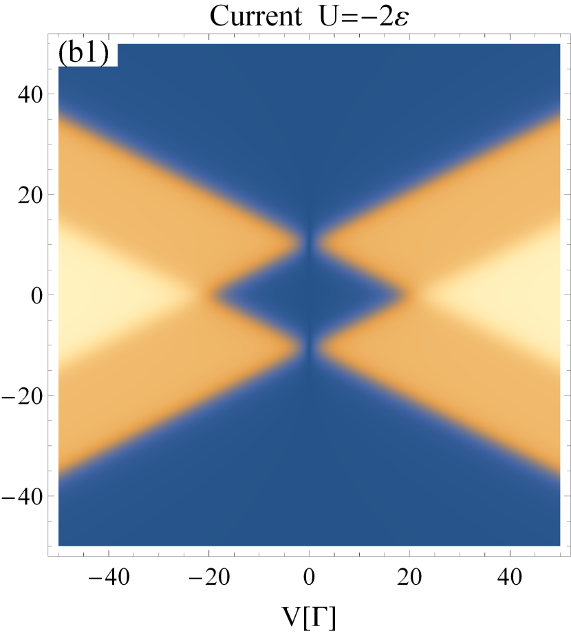
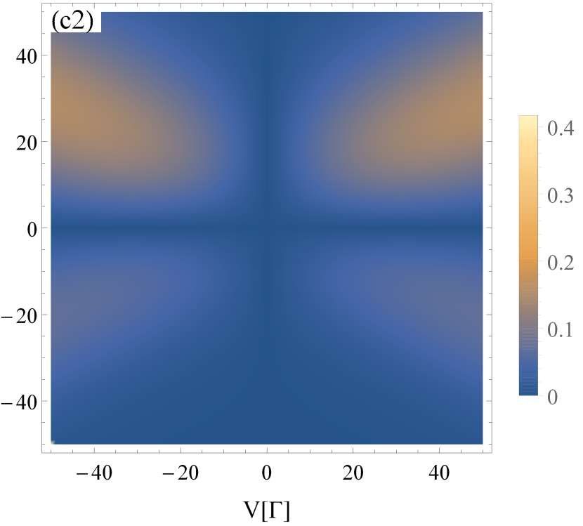
Figure 2: The magnitude of the steady state current as a function of the Fermi-energy $\varepsilon_{f}$ and the bias voltage between the leads $V$. Panels (a1) and (a2) are for the noninteracting system, $U=0$. Panels (b1) and (b2) are for the interacting system with $U=-2\varepsilon$. Panels (c1) and (c2) display the absolute value of the difference between the interacting and noninteracting results. Upper and lower panels were computed for $T_{\rm L}=T_{\rm R}=\Gamma$ and $T_{\rm L}=T_{\rm R}=10\Gamma$, respectively. Other parameters used: $\Gamma_{\rm L}=\Gamma_{\rm R}=\Gamma/2$, and $\varepsilon=-10\Gamma$.

In Fig. 2 we plot the magnitude of the current for the noninteracting (left panels) and interacting (middle panels) models, $I_{{\rm L}}^{(0)}$ and $I_{{\rm L}}^{(U)}$, respectively. The results are plotted as a function of the Fermi energy ($\varepsilon_{f}$) and the bias voltage applied between the leads ($V=\mu_{L}-\mu_{R}$), with the chemical potentials of the leads set to $\mu_{{}_{\rm L,R}}=\varepsilon_{f}\pm V/2$. Two different temperatures were considered: $T_{\rm L}=T_{\rm R}=\Gamma$ (upper panels) and $T_{\rm L}=T_{\rm R}=10\Gamma$ (lower panels). To directly compare the results between the interacting and noninteracting models, we also plot the absolute value of the difference between the two (right panels). Results are shown for the EOM-NEGF approach, but a similar qualitative picture emerges within the QME formalism.

Focusing on the results for the noninteracting system (Fig. 2, panels (a1) and (a2)), as expected, we find significant values for the current at a finite bias when $\varepsilon_{f}-\varepsilon<|V|/2$, leading to the well-known diamond-like current characteristics, broadened by the temperature $T$. The picture is a bit more evolved for the interacting case (Fig. 2, panels (b1) and (b2)), where a double diamond-like current characteristic shape is observed for $U=-2\varepsilon$. The two-step value of the current results from the well-known Coulomb blockade, where the bias voltage is not sufficiently large to overcome the onsite repulsion, and only one conductance channel is open at intermediate bias voltage values. Only when $|V|$ becomes sufficiently large compared to $U$ an additional conducting channel opens up, and consequently the current increases to its maximal value. We note that the Coulomb blockade phenomenon is suppressed in the high temperature limit, as would be expected, where the current rises gradually to its maximum value.

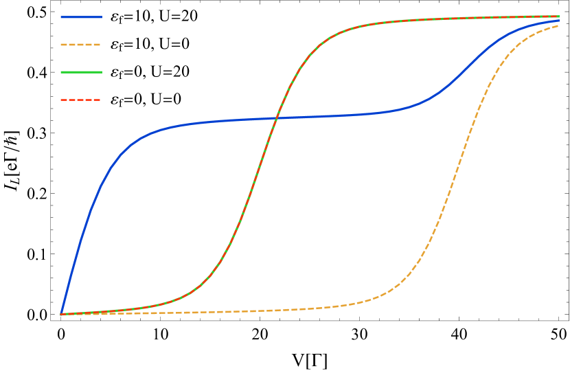
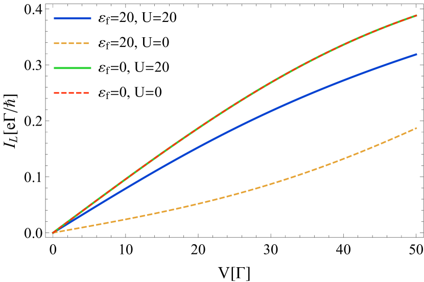
Figure 3: Magnitude of the steady state current as a function of bias voltage at and away from the symmetric point for a) the low temperature conditions in Fig.2 (a1) and (b1) and b) the high temperature conditions in Fig.2 (a2) and (b2). The solid lines denote the Anderson model, whereas the dashed lines denote the noninteracting model.

Interestingly, when the bias voltage is applied symmetrically, i.e. $\varepsilon_{f}=0$, we find that the current-voltage characteristics are identical for both interacting and noninteracting models, suggesting that the Coulomb blockade is completely suppressed. This is clearly depicted in panels (c1) and (c2) of Fig. 2, where we plot the difference between the interacting and noninteracting currents, which diminishes as we approach the line $\varepsilon_{f}=0$ for all values of $V$. This is clarified in Fig. 3 where we show cuts through the 2D plots of Fig. 2 for two values of $\varepsilon_{f}$. When $\varepsilon_{f}\neq 0$, the I-V curves differ at both intermediate and high temperatures, while for a symmetric bias, $\varepsilon_{f}=0$, the interacting and noninteracting results overlap irrespective of the value of $T$. The results for $\varepsilon_{f}=0$ for different values of $U$ and $\varepsilon$ are summarized in Fig. 4, where we plot the difference between the interacting and noninteracting currents for a fixed bias voltage of $V=4\Gamma$. The green dashed line indicates the symmetric line where $U=-2\varepsilon$, for which the difference between the currents vanishes.

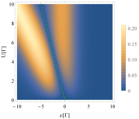
Figure 4: The absolute value of the difference between the steady-state currents of the interacting and noninteracting models at $\varepsilon_{f}=0$ and $V=4\Gamma$ for a range of gate voltages, $\varepsilon$ and onsite Hubbard interaction strength, $U$. The green dashed line represents the symmetric line defined by $U=-2\varepsilon$, where the difference between the two currents vanishes. Other parameters used: $\Gamma_{\rm L}=\Gamma_{\rm R}=\Gamma/2$, and $T_{\rm L}=T_{\rm R}=\Gamma$.

We now turn to rationalize this result. We begin by using the QME approach, which provides a simple relation between the interacting and noninteracting currents at $\varepsilon_{f}=0$. In the case where $\mu_{\rm L}=-\mu_{\rm R}\equiv\mu$ the master equation has a rather simple exact solution for the steady-state populations and currents (see supporting information). The steady-state current is given by

$$I_{\rm L}^{\left(U=0\right)}=\frac{2e\Gamma_{\rm L}\Gamma_{\rm R}}{\Gamma_{\rm L}+\Gamma_{\rm R}}\left(f^{\rm L}(\varepsilon-\mu)-f^{\rm R}(\varepsilon+\mu)\right),$$ (15)

for the noninteracting case, whereas for the symmetric interacting model, the current takes a slightly more complicated form:

$$I_{\rm L}^{\left(U=-2\varepsilon\right)}=\frac{2e\Gamma_{L}\Gamma_{R}\left(f^{\rm L}(\varepsilon-\mu)f^{\rm R}(\varepsilon-\mu)-f^{\rm L}(\varepsilon+\mu)f^{\rm R}(\varepsilon+\mu)\right)}{\Gamma_{\rm L}\left(f^{\rm L}(\varepsilon-\mu)+f^{\rm L}(\varepsilon+\mu)\right)+\Gamma_{\rm R}\left(f^{\rm R}(\varepsilon-\mu)+f^{R}(\varepsilon+\mu)\right)}.$$ (16)

When the temperatures of both leads are balanced, i.e. $T_{\rm L}=T_{\rm R}$, Eqs. (15) and (16) coincide exactly. Note that the leads’ spectral functions, $\Gamma_{\rm L}$ and $\Gamma_{\rm R}$, need not be equal and the two expressions coincide as long as $\Gamma_{L}$ and $\Gamma_{R}$ are even functions in energy. In the case where $\Gamma_{\rm L}=\Gamma_{\rm R}$, we obtain half-filling of the dot, i.e., $n_{\uparrow}\big{|}_{U=-2\varepsilon}=n_{\downarrow}\big{|}_{U=-2\varepsilon}=\frac{1}{2}$. Furthermore, the probabilities of the symmetric model are directly related to the non-interacting system average populations by:

$$n_{\uparrow}\big{|}_{\begin{subarray}{c}U=0\end{subarray}} = n_{\downarrow}\big{|}_{U=0}=2p_{\uparrow}\big{|}_{\begin{subarray}{c}U=-2\varepsilon\end{subarray}}=2p_{\downarrow}\big{|}_{\begin{subarray}{c}U=-2\varepsilon\end{subarray}}=\frac{f(\varepsilon-\mu)+f(\varepsilon+\mu)}{2}$$ (17)

$$(1-n_{\uparrow})\big{|}_{\begin{subarray}{c}U=0\end{subarray}} = (1-n_{\downarrow})\big{|}_{U=0}=2p_{0}\big{|}_{\begin{subarray}{c}U=-2\varepsilon\end{subarray}}=2p_{f}\big{|}_{\begin{subarray}{c}U=-2\varepsilon\end{subarray}}=1-\frac{f(\varepsilon-\mu)+f(\varepsilon+\mu)}{2}.$$

One additional consequence of having the same electric currents is that the steady-state entropy production will also coincide exactly for the two models at this special symmetric point for $\varepsilon_{f}=0$.

The equivalence between the interacting and noninteracting currents can also be derived within the EOM-NEGF approach. For clarity, we restrict the discussion to the wide band limit and assume that $\Gamma_{\rm L}=\Gamma_{\rm R}=\Gamma/2$. In this limit, we find that the difference between the steady state currents of the interacting and noninteracting models is given by (see supporting information):

$$I_{\rm L}^{\left(U=-2\varepsilon\right)}-I_{\rm L}^{\left(U=0\right)}=e\Gamma^{2}U\frac{\left\langle n_{\uparrow}\right\rangle+\left\langle n_{\downarrow}\right\rangle}{2}\int_{-\infty}^{\infty}\frac{d\omega}{2\pi}\frac{2\omega\left(f^{\rm L}\left(\omega-\mu_{\rm L}\right)-f^{\rm R}\left(\omega-\mu_{\rm R}\right)\right)}{\omega^{4}+2\omega^{2}\left(\left(\frac{\Gamma}{2}\right)^{2}-\left(\frac{U}{2}\right)^{2}\right)+\left(\left(\frac{\Gamma}{2}\right)^{2}+\left(\frac{U}{2}\right)^{2}\right)^{2}}.$$ (18)

When the electric bias is centred around $\varepsilon_{f}=0$ with $T_{\rm L}=T_{\rm R}$, the above difference vanishes exactly, as the integrand becomes an odd function of $\omega$.

4 Conclusions

In conclusion, we have shown that the current in the Coulomb blockade regime for a symmetric Anderson impurity model is identical to the current in a non-interacting model. This was demonstrated (numerically and analytically) within the quantum master equation approach as well as the equation of motion NEGF approach (within a two-particle closure) for a wide range of model parameters, bias voltages, and temperatures. The Anderson impurity model is the canonical model to study weakly and strongly correlated effects away from equilibrium and is routinely used to assess the accuracy of approximate methods to compute the dynamics and steady-state properties. Limiting such assessments to the special symmetric point, as described in this work, is by no means a signature of a valid many-body approximation. Such methods should always be tested away from the symmetric case.

The authors would like to thank Wenjie Dou and Guy Cohen for fruitful discussions. M.T. thanks Eran Rabani for kindly hosting his sabbatical stay at the Chemistry Department of the University of California at Berkeley and acknowledges support by the German Research Foundation (DFG). J.O. acknowledges support from the Georg H. Endress foundation. This work was supported by the U.S. Department of Energy, Office of Science, Office of Basic Energy Sciences, Materials Sciences and Engineering Division, under Contract No. DEAC02-05-CH11231 within the Physical Chemistry of Inorganic Nanostructures Program (KC3103).

In this supporting information we give a detailed derivation of the master equation and the equation of motion approach to the nonequilibrium Green’s functions for the Anderson impurity model and assess the validity of these approximations.

The Anderson impurity model is defined by the Hamiltonian $H=H_{S}+H_{B}+V$, where

$$H_{S}= \sum_{\sigma}\varepsilon_{\sigma}d_{\sigma}^{\dagger}d_{\sigma}+Ud_{\uparrow}^{\dagger}d_{\uparrow}d_{\downarrow}^{\dagger}d_{\downarrow}$$ (19)

describes the impurity (or dot), referred to simply as the ‘system Hamiltonian’,

$$H_{B}= \sum_{\underset{k\in L,R}{\sigma=\uparrow,\downarrow}}\varepsilon_{k}c_{k\sigma}^{\dagger}c_{k\sigma}$$ (20)

describes the noninteracting fermionic baths (or leads), and

$$V= \sum_{\underset{k\in L,R}{\sigma=\uparrow,\downarrow}}t_{k}d_{\sigma}^{\dagger}c_{k\sigma}+{\rm h.c.},$$ (21)

describes the hybridization between the system and the leads. In the above, $d_{\sigma}^{\dagger}\ \left(d_{\sigma}\right)$ are the creation (annihilation) operators of an electron on the dot with spin $\sigma=\uparrow,\downarrow$ with one-body energy of $\varepsilon_{\sigma}$, $U$ is the on-site Hubbard interaction, $c_{k\sigma}^{\dagger}\ \left(c_{k\sigma}\right)$ are the creation (annihilation) operators of an electron in mode $k$ of the leads with energy $\varepsilon_{k}$, and $t_{k}$ is the hybridization between the dot and mode $k$ in the lead. The coupling to the quasi-continuous leads is modeled by the leads’ spectral function, $\Gamma_{\ell}\left(\omega\right)$, where $t_{k\in\ell}=\sqrt{\Gamma_{\ell}\left(\varepsilon_{k}\right)\Delta\omega/2\pi}$ is the coupling between the dot and the $k$th mode of the $\ell=L,R$ bath, and $\Delta\omega$ is the discretization of the leads energy spectrum. Throughout, we take Planck’s constant and the Boltzmann factor to be 1.

5 Master equation approach

For weak coupling to the leads and at high temperatures, the master equation (ME) approach is an adequate approximation to describe transport in the Anderson impurity model. In the many-body state basis of the system, the ME reduces to the rate equation:

$$\left(\begin{array}[]{c}\dot{p}_{0}\\ \dot{p}_{\uparrow}\\ \dot{p}_{\downarrow}\\ \dot{p}_{f}\end{array}\right)=M\left(\begin{array}[]{c}p_{0}\\ p_{\uparrow}\\ p_{\downarrow}\\ p_{f}\end{array}\right),$$ (22)

where $p_{0}$ is the probability of occupying the empty dot state $\left|0\right>$ , $p_{\uparrow}$ and $p_{\downarrow}$ are the probabilities of occupying a single electron in the states $\left|\uparrow\right>$ and $\left|\downarrow\right>$ respectively, and $p_{f}$ is the probability of having a fully occupied dot corresponding to the state $\left|f\right>$. The transition matrix is given by :

$$M=\sum_{\ell\in L,R}\left(\begin{array}[]{cccc}-\left(\gamma^{\ell}_{\uparrow 0}+\gamma^{\ell}_{\downarrow 0}\right)&\gamma^{\ell}_{0\uparrow}&\gamma^{\ell}_{0\downarrow}&0\\ \gamma^{\ell}_{\uparrow 0}&-\left(\gamma^{\ell}_{0\uparrow}+\gamma^{\ell}_{f\uparrow}\right)&0&\gamma^{\ell}_{\uparrow f}\\ \gamma^{\ell}_{\downarrow 0}&0&-\left(\gamma^{\ell}_{0\downarrow}+\gamma^{\ell}_{f\downarrow}\right)&\gamma_{\downarrow f}\\ 0&\gamma^{\ell}_{f\uparrow}&\gamma^{\ell}_{f\downarrow}&-\left(\gamma^{\ell}_{\uparrow f}+\gamma^{\ell}_{\downarrow f}\right)\end{array}\right).$$ (23)

Here $\gamma^{\ell}_{ij}$ is the transition rate from state $j$ to state $i$ induced by the $\ell=L,R$ bath, which can be calculated using Fermi’s golden rule. Assuming symmetry between spin up and spin down and in the wide-band approximation, the rates are given explicitly by:

$$\gamma^{\ell}_{\uparrow 0} = \gamma^{\ell}_{\downarrow 0}\equiv\gamma^{\ell}(\varepsilon-\mu_{\ell})=\Gamma_{\ell}f^{\ell}(\varepsilon-\mu_{\ell})$$ (24)

$$\gamma^{\ell}_{0\uparrow} = \gamma^{\ell}_{0\downarrow}\equiv\gamma^{\ell}(-\varepsilon+\mu_{\ell})=\Gamma_{\ell}f^{\ell}(-\varepsilon+\mu_{\ell})$$

$$\gamma^{\ell}_{f\uparrow} = \gamma^{\ell}_{f\downarrow}\equiv\gamma^{\ell}(\varepsilon+U-\mu_{\ell})=\Gamma_{\ell}f^{\ell}(\varepsilon+U-\mu_{\ell})$$

$$\gamma^{\ell}_{\uparrow f} = \gamma^{\ell}_{\downarrow f}\equiv\gamma^{\ell}(-\varepsilon-U+\mu_{\ell})=\Gamma_{\ell}f^{\ell}(-\varepsilon-U+\mu_{\ell}),$$

where $\mu_{\ell}$ is the chemical potential for the left ($\ell=L$) or right ($\ell=R$) leads.

The electric, the energy and the heat currents from the $\ell$-bath are given by

$$I_{\ell}(t) = \frac{e}{2}\sum_{ij}\left(N_{i}-N_{j}\right)j_{ij}^{\ell}$$ (25)

$$I^{E}_{\ell}(t) = \frac{1}{2}\sum_{ij}\left(E_{i}-E_{j}\right)j_{ij}^{\ell}$$

$$I^{H}_{\ell}(t) = I^{E}_{\ell}(t)-\mu_{\ell}I_{\ell}(t).$$

where $\quad j_{ij}^{\ell}=\gamma_{ij}^{\ell}p_{j}(t)-\gamma_{ji}^{\ell}p_{i}(t)$. Here $N_{i}$ and $E_{i}$ are the number of electrons and the energy of the many-body state $i$, and $j_{ij}^{\ell}$ is the probability current from state $j$ to state $i$ induced by the coupling to the $\ell$ bath. The probability currents can then be expressed as:

$$j_{\uparrow 0}^{\ell} = \gamma_{\uparrow 0}^{\ell}(\varepsilon-\mu_{\ell})p_{0}(t)-\gamma_{\uparrow 0}^{\ell}(-\varepsilon+\mu_{\ell})p_{\uparrow}(t)$$ (26)

$$j_{\downarrow 0}^{\ell} = \gamma_{\downarrow 0}^{\ell}(\varepsilon-\mu_{\ell})p_{0}(t)-\gamma_{\downarrow 0}^{\ell}(-\varepsilon+\mu_{\ell})p_{\downarrow}(t)$$

$$j_{f\uparrow}^{\ell} = \gamma_{f\uparrow}^{\ell}(\varepsilon+U-\mu_{\ell})p_{\uparrow}(t)-\gamma_{f\uparrow}^{\ell}(-\varepsilon-U+\mu_{\ell})p_{f}(t)$$

$$j_{f\downarrow}^{\ell} = \gamma_{f\downarrow}^{\ell}(\varepsilon+U-\mu_{\ell})p_{\downarrow}(t)-\gamma_{f\downarrow}^{\ell}(-\varepsilon-U+\mu_{\ell})p_{f}(t).$$

Note that if the left and right temperature of the baths are equal $(T_{L}=T_{R})$ and the electric currents of the two systems are the same, then the entropy production $\Delta S$ of the two systems at steady-state is also identical. At steady-state $\Delta S=-\sum_{\ell}\frac{I_{\ell}^{H}}{T_{\ell}}$. Since $T_{L}=T_{R}$ the entropy production depends solely on the electric current.

In the following we assume $\mu_{L}=-\mu_{R}\equiv\mu$.

5.1 Noninteracting model, $U=0$:

Solving equations (22)-(24) for the noninteracting system, the steady-state probabilities are given by:

$$p_{0}(\infty) = \frac{\left(\gamma^{L}(-\varepsilon+\mu)+\gamma^{R}(-\varepsilon-\mu)\right)^{2}}{\left(\Gamma_{L}+\Gamma_{R}\right)^{2}}$$ (27)

$$p_{f}(\infty) = \frac{\left(\gamma^{L}(\varepsilon-\mu)+\gamma^{R}(\varepsilon+\mu)\right)^{2}}{\left(\Gamma_{L}+\Gamma_{R}\right)^{2}}$$

$$p_{\uparrow/\downarrow}(\infty) = \frac{\left(\gamma^{L}(-\varepsilon+\mu)+\gamma^{R}(-\varepsilon-\mu)\right)\left(\gamma^{L}(\varepsilon-\mu)+\gamma^{R}(\varepsilon+\mu)\right)}{\left(\Gamma_{L}+\Gamma_{R}\right)^{2}}.$$

Since spin up and down are independent, the single particle probabilities are simply $q_{0}=\sqrt{p_{0}}$ of having no electron and $q_{1}=\sqrt{p_{f}}$ of having a single electron. Thus, the occupation number (average population) is given by,

$$n_{\uparrow}=n_{\downarrow}=\frac{\gamma^{L}(\varepsilon-\mu)+\gamma^{R}(\varepsilon+\mu)}{\Gamma^{L}+\Gamma^{R}}\bigg{|}_{\begin{subarray}{c}T_{l}=T_{r}\\ \Gamma_{L}=\Gamma_{R}\end{subarray}}=\frac{f(\varepsilon-\mu)+f(\varepsilon+\mu)}{2}.$$ (28)

The steady-state current can be calculated using equations (25) and (26), and is given by

$$I_{L}(\infty)=-I_{R}(\infty)=\frac{2\Gamma_{L}\Gamma_{R}}{\Gamma_{L}+\Gamma_{R}}\left(f^{L}(\varepsilon-\mu)-f^{R}(\varepsilon+\mu)\right).$$ (29)

5.2 Interacting model, symmetric Anderson model $U=-2\varepsilon$:

The steady state probabilities from equations (22)-(24) are

$$p_{0}(\infty) = \frac{\left(\gamma^{L}(\varepsilon+\mu)+\gamma^{R}(\varepsilon-\mu)\right)\left(\Gamma_{L}+\Gamma_{R}-\gamma^{L}(\varepsilon-\mu)-\gamma^{R}(\varepsilon+\mu)\right)}{\left(\Gamma_{L}+\Gamma_{R}\right)\left(\gamma^{L}(\varepsilon-\mu)+\gamma^{L}(\varepsilon+\mu)+\gamma^{R}(\varepsilon-\mu)+\gamma^{R}(\varepsilon+\mu)\right)}$$ (30)

$$p_{f}(\infty) = \frac{\left(\Gamma_{L}+\Gamma_{R}-\gamma^{L}(\varepsilon+\mu)-\gamma^{R}(\varepsilon-\mu)\right)\left(\gamma^{L}(\varepsilon-\mu)+\gamma^{R}(\varepsilon+\mu)\right)}{\left(\Gamma_{L}+\Gamma_{R}\right)\left(\gamma^{L}(\varepsilon-\mu)+\gamma^{L}(\varepsilon+\mu)+\gamma^{R}(\varepsilon-\mu)+\gamma^{R}(\varepsilon+\mu)\right)}$$

$$p_{\uparrow/\downarrow}(\infty) = \frac{\left(\gamma^{L}(\varepsilon+\mu)+\gamma^{R}(\varepsilon-\mu)\right)\left(\gamma^{L}(\varepsilon-\mu)+\gamma^{R}(\varepsilon+\mu)\right)}{\left(\Gamma_{L}+\Gamma_{R}\right)\left(\gamma^{L}(\varepsilon-\mu)+\gamma^{L}(\varepsilon+\mu)+\gamma^{R}(\varepsilon-\mu)+\gamma^{R}(\varepsilon+\mu)\right)}.$$

The additional necessary condition for having half-filling is that $\Gamma_{L}=\Gamma_{R}$ and $T_{L}=T_{R}$. In this case, Eq. (30) can be simplified to yield:

$$p_{0}(\infty) = p_{f}(\infty)=\frac{f(-\varepsilon+\mu)+f(-\varepsilon-\mu)}{4}$$ (31)

$$p_{\uparrow}(\infty) = p_{\downarrow}(\infty)=\frac{f(\varepsilon-\mu)+f(\varepsilon+\mu)}{4},$$

and the occupation number is $n_{\uparrow}=n_{\downarrow}=\frac{1}{2}$. The probabilities $q_{0}$ and $q_{1}$ of the noninteracting system are exactly twice the probabilities of the symmetric interacting system, i.e., $q_{0}=2p_{0}=2p_{f}$ and $q_{1}=2p_{\uparrow}=2p_{\downarrow}$.

Using equations (25), (26) and (30) the steady-state current from the left lead is,

$$I_{L}(\infty)=\frac{2\Gamma_{L}\Gamma_{R}\left(f^{L}(\varepsilon-\mu)f^{R}(\varepsilon-\mu)-f^{L}(\varepsilon+\mu)f^{R}(\varepsilon+\mu)\right)}{\Gamma_{L}\left(f^{L}(\varepsilon-\mu)+f^{L}(\varepsilon+\mu)\right)+\Gamma_{R}\left(f^{R}(\varepsilon-\mu)+f^{R}(\varepsilon+\mu)\right)}$$ (32)

For $T_{L}=T_{R}\equiv T$ the steady-state current takes the form

$$I_{L}(\infty)=-I_{R}(\infty)=\frac{2\Gamma_{L}\Gamma_{R}}{\Gamma_{L}+\Gamma_{R}}\left(f(\varepsilon-\mu)-f(\varepsilon+\mu)\right),$$ (33)

which is identical to the current in the noninteracting model Eq. (29).

In summary, the conditions for having equal currents for the interacting and noninteracting systems are: equal temperatures of the left and right leads $T_{L}=T_{R}$, Fermi energy equal to zero $\mu_{L}=-\mu_{R}$ (symmetric distribution of the bias) and $U=-2\varepsilon$. Note that the leads’ spectral functions, $\Gamma_{L}$ and $\Gamma_{R}$, are not necessarily equal as required for obtaining half-filling, but must be an even function in energy.

As a side note we mention that the difference between the currents in the symmetric and noninteracting models may be expanded to first order in the temperature difference between the leads, $\Delta T=T_{R}-T_{L}$, to obtain

$$I_{L}^{\left(U=-2\varepsilon\right)}-I_{L}^{\left(U=0\right)}=\frac{\Gamma\left(\varepsilon+\varepsilon\cosh\left(\frac{\varepsilon}{T_{L}}\right)\cosh\left(\frac{\mu}{T_{L}}\right)-\mu\sinh\left(\frac{\varepsilon}{T_{L}}\right)\sinh\left(\frac{\mu}{T_{L}}\right)\right)}{2\left(\cosh\left(\frac{\varepsilon}{T_{L}}\right)+\cosh\left(\frac{\mu}{T_{L}}\right)\right)^{2}}\frac{\Delta T}{T_{L}^{2}}.$$ (34)

Thus, one may use the noninteracting result to obtain the interacting current in the vicinity of the symmetry point.

6 Nonequilibrium Green’s function approach

We begin by defining the impurity one-body nonequilibrium Green’s function (GF) on the Keldysh contour, ^{43, 44}

$$G_{\sigma}\left(\tau,\tau^{\prime}\right)=-i\left\langle\hat{T}_{c}\left[d_{\sigma}\left(\tau\right)d_{\sigma}^{\dagger}\left(\tau^{\prime}\right)\right]\right\rangle$$ (35)

where $\hat{T}_{c}$ is the contour ordering operator. Using the equation of motion (EOM) technique ^{54, 55, 48}, we take the derivative of the GF according to one of the contour times, producing the following equation

$$i\frac{\partial G_{\sigma}\left(\tau,\tau^{\prime}\right)}{\partial\tau}=\delta_{c}\left(\tau-\tau^{\prime}\right)+\varepsilon_{\sigma}G_{\sigma}\left(\tau,\tau^{\prime}\right)+UG_{\sigma}^{\left(2\right)}\left(\tau,\tau^{\prime}\right)+\sum_{k\in L,R}t_{k}F_{k\sigma}\left(\tau,\tau^{\prime}\right),$$ (36)

where we defined

$$G_{\sigma}^{\left(2\right)}\left(\tau,\tau^{\prime}\right) =-i\left\langle\hat{T}_{c}\left[d_{\sigma}\left(\tau\right)n_{\bar{\sigma}}\left(\tau\right)d_{\sigma}^{\dagger}\left(\tau^{\prime}\right)\right]\right\rangle,$$ (37)

$$F_{k\sigma}\left(\tau,\tau^{\prime}\right) =-i\left\langle\hat{T}_{c}\left[c_{k\sigma}\left(\tau\right)d_{\sigma}^{\dagger}\left(\tau^{\prime}\right)\right]\right\rangle.$$ (38)

The above satisfy the following equations of motion

$$i\frac{\partial G_{\sigma}^{\left(2\right)}\left(\tau,\tau^{\prime}\right)}{\partial\tau^{\prime}} =-\delta\left(\tau-\tau^{\prime}\right)\left\langle n_{\bar{\sigma}}\left(\tau\right)\right\rangle-\varepsilon_{\sigma}G_{\sigma}^{\left(2\right)}\left(\tau,\tau^{\prime}\right)-UG_{\sigma}^{\left(3\right)}\left(\tau,\tau^{\prime}\right)-\sum_{k\in L,R}t_{k}^{*}F_{k\sigma}^{\left(2\right)}\left(\tau,\tau^{\prime}\right),$$ (39)

$$i\frac{\partial F_{k\sigma}}{\partial\tau}\left(\tau,\tau^{\prime}\right) =\varepsilon_{k\sigma}F_{k\sigma}\left(\tau,\tau^{\prime}\right)+t_{k}^{*}G_{\sigma}\left(\tau,\tau^{\prime}\right),$$ (40)

where we also defined

$$G_{\sigma}^{\left(3\right)}\left(\tau,\tau^{\prime}\right) =-i\left\langle\hat{T}_{c}\left[d_{\sigma}\left(\tau\right)n_{\bar{\sigma}}\left(\tau\right)d_{\sigma}^{\dagger}\left(\tau^{\prime}\right)n_{\bar{\sigma}}\left(\tau^{\prime}\right)\right]\right\rangle,$$ (41)

$$F_{k\sigma}^{\left(2\right)}\left(\tau,\tau^{\prime}\right) =-i\left\langle\hat{T}_{c}\left[d_{\sigma}\left(\tau\right)n_{\bar{\sigma}}\left(\tau\right)c_{k\sigma}^{\dagger}\left(\tau^{\prime}\right)\right]\right\rangle.$$ (42)

Since the Anderson model is not analytically solvable, this ever-growing set of inter-dependent equations will not come to a close, and so, we choose an appropriate closure, which is known to be a good approximation in the Coulomb blockade regime. Within this closure, the equation of motion for $F_{k\sigma}^{\left(2\right)}\left(\tau,\tau^{\prime}\right)$ is taken exactly,

$$i\frac{\partial F_{k\sigma}^{\left(2\right)}\left(\tau,\tau^{\prime}\right)}{\partial\tau^{\prime}} =-\varepsilon_{k\sigma}F_{k\sigma}^{\left(2\right)}\left(\tau,\tau^{\prime}\right)-t_{k}G_{\sigma}^{\left(2\right)}\left(\tau,\tau^{\prime}\right),$$ (43)

whereas $G_{\sigma}^{\left(3\right)}\left(\tau,\tau^{\prime}\right)$ is treated approximately. If one derives the EOM for $G_{\sigma}^{\left(2\right)}\left(\tau,\tau^{\prime}\right)$ under the noninteracting, uncoupled Hamiltonian, the resulting equation of motion is found to be identical to that of $G_{\sigma}^{\left(3\right)}\left(\tau,\tau^{\prime}\right)$ under the same Hamiltonian (and has the same initial value). Therefore, within this closure, we will use the approximation:

$$G_{\sigma}^{\left(3\right)}\left(\tau,\tau^{\prime}\right)\simeq G_{\sigma}^{\left(2\right)}\left(\tau,\tau^{\prime}\right).$$ (44)

In this derivation, we will also consider the neglected terms from the closure, in order to keep the full description in mind. Thus, we define

$$G_{\sigma}^{\left(3\right)}=G_{\sigma}^{\left(2\right)}+\Gamma F_{\sigma}^{\left({\rm corr}\right)},$$ (45)

where $\Gamma F_{\sigma}^{\left({\rm corr}\right)}$ is the difference between the exact $G_{\sigma}^{\left(3\right)}$ and our approximation and the leading contribution due to the coupling to the leads is factored out. As a side note, we can show that the correction term will contribute at least $\propto\Gamma$ by writing out the full equation of motion for $G_{\sigma}^{\left(3\right)}$,

$$i\frac{\partial G_{\sigma}^{\left(3\right)}\left(\tau,\tau^{\prime}\right)}{\partial\tau} = \frac{\partial}{\partial\tau}\left[\theta\left(\tau-\tau^{\prime}\right)\left\langle\left\{d_{\sigma}\left(\tau\right)n_{\bar{\sigma}}\left(\tau\right),d_{\sigma}^{\dagger}\left(\tau^{\prime}\right)n_{\bar{\sigma}}\left(\tau^{\prime}\right)\right\}\right\rangle\right]$$

$$= \delta\left(\tau-\tau^{\prime}\right)\left\langle n_{\bar{\sigma}}\left(\tau\right)\right\rangle+\left\langle\hat{T}_{c}\left[\dot{d}_{\sigma}\left(\tau\right)n_{\bar{\sigma}}\left(\tau\right)d_{\sigma}^{\dagger}\left(\tau^{\prime}\right)n_{\bar{\sigma}}\left(\tau^{\prime}\right)\right]\right\rangle$$

$$+\left\langle\hat{T}_{c}\left[d_{\sigma}\left(\tau\right)\dot{n}_{\bar{\sigma}}\left(\tau\right)d_{\sigma}^{\dagger}\left(\tau^{\prime}\right)n_{\bar{\sigma}}\left(\tau^{\prime}\right)\right]\right\rangle$$

$$= \delta\left(\tau-\tau^{\prime}\right)\left\langle n_{\bar{\sigma}}\left(\tau\right)\right\rangle$$

$$-i\left\langle\hat{T}_{c}\left[\left(\varepsilon_{\sigma}d_{\sigma}\left(\tau\right)+Ud_{\sigma}\left(\tau\right)n_{\bar{\sigma}}\left(\tau\right)+\sum_{k\in L,R}t_{k}c_{k\sigma}\left(\tau\right)\right)n_{\bar{\sigma}}\left(\tau\right)d_{\sigma}^{\dagger}\left(\tau^{\prime}\right)n_{\bar{\sigma}}\left(\tau^{\prime}\right)\right]\right\rangle$$

$$-i\left\langle\hat{T}_{c}\left[d_{\sigma}\left(t\right)\left(\sum_{k\in L,R}t_{k}d_{\sigma}^{\dagger}\left(t\right)c_{k\sigma}\left(t\right)+\sum_{k\in L,R}t_{k}d_{\sigma}\left(t\right)c_{k\sigma}^{\dagger}\left(t\right)\right)d_{\sigma}^{\dagger}\left(t^{\prime}\right)n_{\bar{\sigma}}\left(t^{\prime}\right)\right]\right\rangle.$$

To arrive at the uncoupled equation, we neglect all terms with $\sum_{k\in L,R}t_{k}$, keeping only terms that appear in the propagation under the dot Hamiltonian,

$$i\frac{\partial G_{\sigma}^{\left(3\right)}\left(\tau,\tau^{\prime}\right)}{\partial\tau} \simeq \delta\left(\tau-\tau^{\prime}\right)\left\langle n_{\bar{\sigma}}\left(\tau\right)\right\rangle-i\varepsilon_{\sigma}\left\langle\hat{T}_{c}\left[d_{\sigma}\left(\tau\right)n_{\bar{\sigma}}\left(\tau\right)d_{\sigma}^{\dagger}\left(\tau^{\prime}\right)n_{\bar{\sigma}}\left(\tau^{\prime}\right)\right]\right\rangle$$

$$-iU\left\langle\hat{T}_{c}\left[d_{\sigma}\left(\tau\right)n_{\bar{\sigma}}\left(\tau\right)n_{\bar{\sigma}}\left(\tau\right)d_{\sigma}^{\dagger}\left(\tau^{\prime}\right)n_{\bar{\sigma}}\left(\tau^{\prime}\right)\right]\right\rangle$$

$$= \delta\left(\tau-\tau^{\prime}\right)\left\langle n_{\bar{\sigma}}\left(\tau\right)\right\rangle+\left(\varepsilon_{\sigma}+U\right)G_{\sigma}^{\left(3\right)}\left(\tau,\tau^{\prime}\right)$$

thus,

$$G_{\sigma}^{\left(3\right)}\left(\tau,\tau^{\prime}\right) =G_{\sigma}^{\left(2\right)}\left(\tau,\tau^{\prime}\right)+\int_{0}^{\tau}\left[{\rm neglected\ terms}\right]\left(\tau_{1},\tau^{\prime}\right){\rm d}\tau_{1}$$ (46)

$$\equiv G_{\sigma}^{\left(2\right)}\left(\tau,\tau^{\prime}\right)+\Gamma F_{\sigma}^{\left({\rm corr}\right)}.$$

Solving the equations of motion on the Keldysh contour, one arrives at the following integral equations

$$G_{\sigma}\left(\tau,\tau^{\prime}\right)= \,g_{\sigma}^{(0)}\left(\tau,\tau^{\prime}\right)+\iint{\rm d}\tau_{1}{\rm d}\tau_{2}\,g_{\sigma}^{(0)}\left(\tau,\tau_{1}\right)\Sigma_{\ell\sigma}\left(\tau_{1},\tau_{2}\right)G_{\sigma}\left(\tau_{2},\tau^{\prime}\right)$$ (47)

$$+U\int{\rm d}\tau_{1}\,g_{\sigma}^{(0)}\left(\tau,\tau_{1}\right)G_{\sigma}^{\left(2\right)}\left(\tau_{1},\tau^{\prime}\right),$$

$$G_{\sigma}^{\left(2\right)}\left(\tau,\tau^{\prime}\right)= \,g_{\sigma}^{\left(U\right)}\left(\tau,\tau^{\prime}\right)\left\langle n_{\bar{\sigma}}\left(\tau\right)\right\rangle+\iint{\rm d}\tau_{1}{\rm d}\tau_{2}\,G_{\sigma}^{\left(2\right)}\left(\tau,\tau_{2}\right)\Sigma_{\ell\sigma}\left(\tau_{2},\tau_{1}\right)g_{\sigma}^{\left(U\right)}\left(\tau_{1},\tau^{\prime}\right)$$ (48)

$$+U\Gamma\int{\rm d}\tau_{1}\,g_{\sigma}^{\left(U\right)}\left(\tau,\tau_{1}\right)F_{\sigma}^{\left({\rm corr}\right)}\left(\tau_{1},\tau^{\prime}\right),$$

where the noninteracting Green’s function on the contour are defined as

$$g_{\sigma}^{(0)}\left(\tau,\tau^{\prime}\right) =-i\left\langle\hat{T}_{c}\left[d_{\sigma}\left(\tau\right)d_{\sigma}^{\dagger}\left(\tau^{\prime}\right)\right]\right\rangle_{{\rm under}\ H_{0}=\varepsilon_{\sigma}n_{\sigma}},$$ (49)

$$g_{\sigma}^{\left(U\right)}\left(\tau,\tau^{\prime}\right) =-i\left\langle\hat{T}_{c}\left[d_{\sigma}\left(\tau\right)d_{\sigma}^{\dagger}\left(\tau^{\prime}\right)\right]\right\rangle_{{\rm under}\ H_{0}=\left(\varepsilon_{\sigma}+U\right)n_{\sigma}},$$

and the self energy due to the coupling to the leads (identical to the noninteracting model self energy) is given by

$$\Sigma_{\ell\sigma}\left(\tau,\tau^{\prime}\right)=-i\sum_{k\in L,R}\left|t_{k}\right|^{2}\left\langle\hat{T}_{c}\left[c_{k\sigma}\left(\tau\right)c_{k\sigma}^{\dagger}\left(\tau^{\prime}\right)\right]\right\rangle_{{\rm under}\ H_{0}=H_{B}}.$$ (50)

By means of analytical continuation (Langreth rules)⁵², we find that the equations for the retarded and lesser Green’s functions are given by

$$G_{\sigma}^{r}\left(t,t^{\prime}\right)= \,g_{\sigma}^{(0)r}\left(t-t^{\prime}\right)+\iint{\rm d}t_{1}{\rm d}t_{2}\,g_{\sigma}^{(0)r}\left(t-t_{1}\right)\Sigma_{\ell\sigma}^{r}\left(t_{1}-t_{2}\right)G_{\sigma}^{r}\left(t_{2},t^{\prime}\right)$$ (51)

$$+U\int{\rm d}t_{1}\,g_{\sigma}^{(0)r}\left(t-t_{1}\right)G_{\sigma}^{\left(2\right)r}\left(t_{1},t^{\prime}\right),$$

$$G_{\sigma}^{\left(2\right)r}\left(t,t^{\prime}\right)= \,g_{\sigma}^{\left(U\right)r}\left(t-t^{\prime}\right)\left\langle n_{\bar{\sigma}}\left(t\right)\right\rangle+\iint{\rm d}t_{1}{\rm d}t_{2}\,G_{\sigma}^{\left(2\right)r}\left(t,t_{2}\right)\Sigma_{\ell\sigma}^{r}\left(t_{2}-t_{1}\right)g_{\sigma}^{\left(U\right)r}\left(t_{1}-t^{\prime}\right)$$ (52)

$$+U\Gamma\int g_{\sigma}^{\left(U\right)r}\left(t-t_{1}\right)F_{\sigma}^{\left({\rm corr}\right)r}\left(t_{1},t^{\prime}\right)$$

$$G_{\sigma}^{<}\left(t,t^{\prime}\right)= g_{\sigma}^{(0)<}\left(t-t^{\prime}\right)+\iint g_{\sigma}^{(0)r}\left(t-t_{1}\right)\Sigma_{\ell\sigma}^{r}\left(t_{1}-t_{2}\right)G_{\sigma}^{<}\left(t_{2},t^{\prime}\right)$$ (53)

$$+\iint g_{\sigma}^{(0)r}\left(t-t_{1}\right)\Sigma_{\ell\sigma}^{<}\left(t_{1}-t_{2}\right)G_{\sigma}^{a}\left(t_{2},t^{\prime}\right)+\iint g_{\sigma}^{(0)<}\left(t-t_{1}\right)\Sigma_{\ell\sigma}^{a}\left(t_{1}-t_{2}\right)G_{\sigma}^{a}\left(t_{2},t^{\prime}\right)$$

$$+U\int g_{\sigma}^{(0)r}\left(t-t_{1}\right)G_{\sigma}^{\left(2\right)<}\left(t_{1},t^{\prime}\right)+U\int g_{\sigma}^{(0)<}\left(t-t_{1}\right)G_{\sigma}^{\left(2\right)a}\left(t_{1},t^{\prime}\right),$$

$$G_{\sigma}^{\left(2\right)<}\left(t,t^{\prime}\right)= g_{\sigma}^{\left(U\right)<}\left(t-t^{\prime}\right)\left\langle n_{\bar{\sigma}}\left(t\right)\right\rangle+\iint g_{\sigma}^{\left(U\right)r}\left(t-t_{1}\right)\Sigma_{\ell\sigma}^{r}\left(t_{1}-t_{2}\right)G_{\sigma}^{\left(2\right)<}\left(t_{2},t^{\prime}\right)$$ (54)

$$+\iint g_{\sigma}^{\left(U\right)r}\left(t-t_{1}\right)\Sigma_{\ell\sigma}^{<}\left(t_{1}-t_{2}\right)G_{\sigma}^{\left(2\right)a}\left(t_{2},t^{\prime}\right)$$

$$+\iint g_{\sigma}^{\left(U\right)<}\left(t-t_{1}\right)\Sigma_{\ell\sigma}^{a}\left(t_{1}-t_{2}\right)G_{\sigma}^{\left(2\right)a}\left(t_{2},t^{\prime}\right)$$

$$+U\Gamma\int g_{\sigma}^{\left(U\right)r}\left(t-t_{1}\right)F_{\sigma}^{\left({\rm corr}\right)<}\left(t_{1},t^{\prime}\right)+U\Gamma\int g_{\sigma}^{\left(U\right)<}\left(t-t_{1}\right)F_{\sigma}^{\left({\rm corr}\right)a}\left(t_{1},t^{\prime}\right),$$

where the noninteracting Green’s functions are given by

$$g_{\sigma}^{(0)r}\left(t\right) =-i\theta\left(t\right)e^{-i\varepsilon_{\sigma}t},$$ (55)

$$g_{\sigma}^{(0)<}\left(t\right) =ie^{-i\varepsilon_{\sigma}t}n_{\sigma}\left(0\right),$$

$$g_{\sigma}^{\left(U\right)r}\left(t\right) =-i\theta\left(t\right)e^{-i\left(\varepsilon_{\sigma}+U\right)t},$$

$$g_{\sigma}^{\left(U\right)<}\left(t\right) =ie^{-i\left(\varepsilon_{\sigma}+U\right)t}n_{\sigma}\left(0\right),$$

$$\Sigma_{\ell\sigma}^{r}\left(t\right) =-i\theta\left(t\right)\int_{-\infty}^{\infty}\frac{\mbox{d}\omega}{2\pi}\left(\Gamma_{L}\left(\omega\right)+\Gamma_{R}\left(\omega\right)\right)e^{-\frac{i}{\hbar}\omega t}=-i\theta\left(t\right)\Gamma\left(t\right),$$

$$\Sigma_{\ell\sigma}^{<}\left(t\right) =i\int_{-\infty}^{\infty}\frac{\mbox{d}\omega}{2\pi}\left(\Gamma_{L}\left(\omega\right)f_{F}\left(\omega-\mu_{L}\right)+\Gamma_{R}\left(\omega\right)f_{F}\left(\omega-\mu_{R}\right)\right)e^{-\frac{i}{\hbar}\omega t}.$$

In steady state, all functions depend on time differences rather than two time variables, and thus, the integral equation are simplified to algebraic equations in frequency space. Therefore,

$$G_{\sigma}^{r}\left(\omega\right) =g_{\sigma}^{(0)r}\left(\omega\right)+g_{\sigma}^{(0)r}\left(\omega\right)\Sigma_{\sigma}^{r}\left(\omega\right)G_{\sigma}^{r}\left(\omega\right)+Ug_{\sigma}^{(0)r}\left(\omega\right)G_{\sigma}^{\left(2\right)r}\left(\omega\right),$$ (56)

$$G_{\sigma}^{\left(2\right)r}\left(\omega\right) =g_{\sigma}^{\left(U\right)r}\left(\omega\right)\left\langle n_{\bar{\sigma}}\right\rangle+g_{\sigma}^{\left(U\right)r}\left(\omega\right)\Sigma_{\sigma}^{r}\left(\omega\right)G_{\sigma}^{\left(2\right)r}\left(\omega\right)+U\Gamma g_{\sigma}^{\left(U\right)r}\left(\omega\right)F_{\sigma}^{\left({\rm corr}\right)r}\left(\omega\right),$$

$$G_{\sigma}^{<}\left(\omega\right) =g_{\sigma}^{(0)<}\left(\omega\right)+g_{\sigma}^{(0)r}\left(\omega\right)\Sigma_{\sigma}^{r}\left(\omega\right)G_{\sigma}^{<}\left(\omega\right)+g_{\sigma}^{(0)r}\left(\omega\right)\Sigma_{\sigma}^{<}\left(\omega\right)G_{\sigma}^{a}\left(\omega\right)+g_{\sigma}^{(0)<}\left(\omega\right)\Sigma_{\sigma}^{a}\left(\omega\right)G_{\sigma}^{a}\left(\omega\right)$$

$$+Ug_{\sigma}^{(0)r}\left(\omega\right)G_{\sigma}^{\left(2\right)<}\left(\omega\right)+Ug_{\sigma}^{(0)<}\left(\omega\right)G_{\sigma}^{\left(2\right)a}\left(\omega\right),$$

$$G_{\sigma}^{\left(2\right)<}\left(\omega\right) =g_{\sigma}^{\left(U\right)<}\left(\omega\right)\left\langle n_{\bar{\sigma}}\right\rangle+g_{\sigma}^{\left(U\right)r}\left(\omega\right)\Sigma_{\sigma}^{r}\left(\omega\right)G_{\sigma}^{\left(2\right)<}\left(\omega\right)+g_{\sigma}^{\left(U\right)r}\left(\omega\right)\Sigma_{\sigma}^{<}\left(\omega\right)G_{\sigma}^{\left(2\right)a}\left(\omega\right)$$

$$+g_{\sigma}^{\left(U\right)<}\left(\omega\right)\Sigma_{\sigma}^{a}\left(\omega\right)G_{\sigma}^{\left(2\right)a}\left(\omega\right)+U\Gamma g_{\sigma}^{\left(U\right)r}\left(\omega\right)F_{\sigma}^{\left({\rm corr}\right)<}\left(\omega\right)+U\Gamma g_{\sigma}^{\left(U\right)<}\left(\omega\right)F_{\sigma}^{\left({\rm corr}\right)a}\left(\omega\right),$$

where the $\sigma$-spin electron steady state population, $\left\langle n_{\sigma}\right\rangle$ is given by:

$$\left\langle n_{\sigma}\right\rangle=-i\int_{-\infty}^{\infty}\frac{d\omega}{2\pi}G_{\sigma}^{<}\left(\omega\right),$$ (57)

and the noninteracting Green’s functions in frequency are given by

$$g_{\sigma}^{(0)r}\left(\omega\right) =\frac{1}{\omega-\varepsilon_{\sigma}+i\eta},$$ (58)

$$g_{\sigma}^{(0)<}\left(\omega\right) =2\pi\left\langle d^{\dagger}d\right\rangle_{0}\delta\left(\omega-\varepsilon_{\sigma}\right),$$

$$g_{\sigma}^{\left(U\right)r}\left(\omega\right) =\frac{1}{\omega-\varepsilon_{\sigma}-U+i\eta},$$

$$g_{\sigma}^{\left(U\right)<}\left(\omega\right) =2\pi\left\langle d^{\dagger}d\right\rangle_{0}\delta\left(\omega-\varepsilon_{\sigma}-U\right),$$

$$\Sigma_{\sigma}^{r}\left(\omega\right) =-\frac{i}{2}\Gamma\left(\omega\right),$$

$$\Sigma_{\sigma}^{<}\left(\omega\right) =i\left(\Gamma_{L}\left(\omega\right)f\left(\omega-\mu_{L}\right)+\Gamma_{R}\left(\omega\right)f\left(\omega-\mu_{R}\right)\right).$$

In the above, we assumed that the spectral function characterizing the dot-lead coupling is symmetric, i.e. $\Gamma\left(\omega\right)=\Gamma\left(-\omega\right)$. Note we also set the Fermi energy of the leads to $\varepsilon_{f}=0$, and consider spectral functions that are symmetric around $\varepsilon_{f}$. This will be critical for considering the symmetric point of the Anderson model. The above equations may now be solved analytically.

6.1 Symmetric case - steady state solution

Let us now consider the more special case of the symmetric Anderson model, where:

$$\varepsilon_{\uparrow} =\varepsilon_{\downarrow}=-U/2,$$ (59)

$$\varepsilon_{\sigma}+ U=U/2.$$

The noninteracting GFs in steady state take the form:

$$g_{\sigma}^{(0)r}\left(\omega\right) =\frac{1}{\omega+U/2+i\eta},$$ (60)

$$g_{\sigma}^{(0)<}\left(\omega\right) =2\pi\left\langle d^{\dagger}d\right\rangle_{0}\delta\left(\omega+U/2\right),$$

$$g_{\sigma}^{\left(U\right)r}\left(\omega\right) =\frac{1}{\omega-U/2+i\eta},$$

$$g_{\sigma}^{\left(U\right)<}\left(\omega\right) =2\pi\left\langle d^{\dagger}d\right\rangle_{0}\delta\left(\omega-U/2\right).$$

Solving the steady state equations in frequency space, we start with the retarded GF. Rewriting the first line of equation 56, we find

$$G_{\sigma}^{r} =g_{\sigma}^{(0)r}\left(1-g_{\sigma}^{(0)r}\Sigma^{r}\right)^{-1}+g_{\sigma}^{(0)r}\left(1-g_{\sigma}^{(0)r}\Sigma^{r}\right)^{-1}UG_{\sigma}^{\left(2\right)r},$$ (61)

$$=G_{\sigma}^{(0)r}+G_{\sigma}^{(0)r}UG_{\sigma}^{\left(2\right)r},$$

where we recognized the retarded GF for the noninteracting model ⁵³ with $\varepsilon=-\frac{U}{2}$,

$$G_{\sigma}^{(0)r}=\left(\left(g_{\sigma}^{(0)r}\right)^{-1}-\Sigma^{r}\right)^{-1}=\left(\omega+\frac{U}{2}-\Sigma^{r}\right)^{-1}.$$ (62)

Similarly, from the second line of 56, we find:

$$G_{\sigma}^{\left(2\right)r}\left(\omega\right) =g_{\sigma}^{\left(U\right)r}\left(1-g_{\sigma}^{\left(U\right)r}\Sigma^{r}\right)^{-1}\left\langle n_{\bar{\sigma}}\right\rangle+g_{\sigma}^{\left(U\right)r}\left(1-g_{\sigma}^{(U)r}\Sigma^{r}\right)^{-1}U\Gamma F_{\sigma}^{\left({\rm corr}\right)r}$$ (63)

$$=G_{\sigma}^{(0^{\prime})r}\left\langle n_{\bar{\sigma}}\right\rangle+G_{\sigma}^{(0^{\prime})r}U\Gamma F_{\sigma}^{\left({\rm corr}\right)r},$$

where

$$G_{\sigma}^{(0^{\prime})r}=\left(\left(g_{\sigma}^{\left(U\right)r}\right)^{-1}-\Sigma^{r}\right)^{-1}=\left(\omega-\frac{U}{2}-\Sigma^{r}\right)^{-1}$$ (64)

is the retarded GF for the noninteracting model with $\varepsilon=+\frac{U}{2}$.

Plugging the above into equation (62), we find:

$$G_{\sigma}^{r}=G_{\sigma}^{(0)r}+G_{\sigma}^{(0)r}UG_{\sigma}^{(0^{\prime})r}\left\langle n_{\bar{\sigma}}\right\rangle+G_{\sigma}^{\left({\rm corr}\right)r},$$ (65)

where we defined the closure-correction contribution to $G^{r}$:

$$G_{\sigma}^{\left({\rm corr}\right)r}=U^{2}\Gamma G_{\sigma}^{(0)r}G_{\sigma}^{(0^{\prime})r}F_{\sigma}^{\left({\rm corr}\right)r}.$$ (66)

Finally, using

$$G_{\sigma}^{(0)r}\cdot G_{\sigma}^{(0^{\prime})r}= \left(\omega+\frac{U}{2}-\Sigma^{r}\right)^{-1}\cdot\left(\omega-\frac{U}{2}-\Sigma^{r}\right)^{-1}$$ (67)

$$= \frac{1}{\omega^{2}-\left(\frac{U}{2}\right)^{2}-2\omega\Sigma^{r}+\left(\Sigma^{r}\right)^{2}}$$

$$= \frac{1}{\left(\omega-i\frac{\Gamma}{2}\right)^{2}-\left(\frac{U}{2}\right)^{2}},$$

we find

$$G_{\sigma}^{r}-G_{\sigma}^{(0)r} =G_{\sigma}^{(0)r}UG_{\sigma}^{(0^{\prime})r}\left\langle n_{\bar{\sigma}}\right\rangle+G_{\sigma}^{\left({\rm corr}\right)r}$$ (68)

$$=\frac{U\left\langle n_{\bar{\sigma}}\right\rangle}{\left(\omega-i\frac{\Gamma}{2}\right)^{2}-\left(\frac{U}{2}\right)^{2}}+G_{\sigma}^{\left({\rm corr}\right)r}$$

where

$$G_{\sigma}^{\left({\rm corr}\right)r}=G_{\sigma}^{(0)r}UG_{\sigma}^{(0^{\prime})r}U\Gamma F_{\sigma}^{\left({\rm corr}\right)r}=\frac{U^{2}\Gamma F_{\sigma}^{\left({\rm corr}\right)r}}{\left(\omega-i\frac{\Gamma}{2}\right)^{2}-\left(\frac{U}{2}\right)^{2}},$$ (69)

and we took the wide-band limit (WBL) for the lead-dot coupling, $\Sigma^{r}\left(\omega\right)=-\frac{i}{2}\left(\Gamma_{L}+\Gamma_{R}\right)=-\frac{i\Gamma}{2}$.

Next, we look at the lesser GF’s from equation (56):

$$G_{\sigma}^{<}\left(\omega\right)= g_{\sigma}^{(0)<}+g_{\sigma}^{(0)r}\Sigma^{r}G_{\sigma}^{<}+g_{\sigma}^{(0)r}\Sigma^{<}G_{\sigma}^{a}+g_{\sigma}^{(0)<}\Sigma^{a}G_{\sigma}^{a}+g_{\sigma}^{(0)r}UG_{\sigma}^{\left(2\right)<}+g_{\sigma}^{(0)<}UG_{\sigma}^{\left(2\right)a}$$ (70)

$$G_{\sigma}^{\left(2\right)<}\left(\omega\right)= g_{\sigma}^{\left(U\right)<}\left\langle n_{\bar{\sigma}}\right\rangle+g_{\sigma}^{\left(U\right)r}\Sigma^{r}G_{\sigma}^{\left(2\right)<}+g_{\sigma}^{\left(U\right)r}\Sigma^{<}G_{\sigma}^{\left(2\right)a}+g_{\sigma}^{\left(U\right)<}\Sigma^{a}G_{\sigma}^{\left(2\right)a}$$

$$+g_{\sigma}^{\left(U\right)r}U\Gamma F_{\sigma}^{\left({\rm corr}\right)<}+g_{\sigma}^{\left(U\right)<}U\Gamma F_{\sigma}^{\left({\rm corr}\right)a}.$$

Terms of the form $g^{<}\left(1-g^{r}\Sigma^{r}\right)^{-1}$ vanish ²² and we are left with:

$$G_{\sigma}^{<}\left(\omega\right) =G_{\sigma}^{(0)r}\Sigma^{<}G_{\sigma}^{a}+G_{\sigma}^{(0)r}UG_{\sigma}^{\left(2\right)<}$$ (71)

$$G_{\sigma}^{\left(2\right)<}\left(\omega\right) =G_{\sigma}^{(0^{\prime})r}\Sigma^{<}G_{\sigma}^{\left(2\right)a}+G_{\sigma}^{(0^{\prime})r}U\Gamma F_{\sigma}^{\left({\rm corr}\right)<}.$$

By using $G^{a}=\left(G^{r}\right)^{*}$ and equation (63), we find

$$G_{\sigma}^{<}-G_{\sigma}^{(0)<}=U\left\langle n_{\bar{\sigma}}\right\rangle G_{\sigma}^{(0)r}\Sigma^{<}\left(G_{\sigma}^{(0^{\prime})r}\right)^{*}\left(\left(G_{\sigma}^{(0)r}\right)^{*}+G_{\sigma}^{(0^{\prime})r}\right)+G_{\sigma}^{\left({\rm corr}\right)<},$$ (72)

where the lesser GF for the noninteracting model is given by

$$G_{\sigma}^{(0)<}=G_{\sigma}^{(0)r}\Sigma^{<}\left(G_{\sigma}^{(0)r}\right)^{*}\xrightarrow{{\rm WBL}}\frac{i}{2}\Gamma\frac{f\left(\omega-\mu_{L}\right)+f\left(\omega-\mu_{R}\right)}{\left(\omega+\frac{U}{2}\right)^{2}+\left(\frac{\Gamma}{2}\right)^{2}},$$ (73)

and we defined

$$G_{\sigma}^{\left({\rm corr}\right)<}= G_{\sigma}^{(0)r}\Sigma^{<}G_{\sigma}^{\left({\rm corr}\right)r*}+G_{\sigma}^{(0)r}UG_{\sigma}^{(0^{\prime})r}\Sigma^{<}G_{\sigma}^{(0^{\prime})r*}U\Gamma F^{\left({\rm corr}\right)r*}+G_{\sigma}^{(0)r}UG_{\sigma}^{(0)r}U\Gamma F^{\left({\rm corr}\right)<}$$ (74)

$$= U^{2}\Gamma G_{\sigma}^{(0)r}\Sigma^{<}G_{\sigma}^{(0^{\prime})r*}\left(G_{\sigma}^{(0)r*}+G_{\sigma}^{(0^{\prime})r}\right)F^{\left({\rm corr}\right)r*}+U^{2}\Gamma G_{\sigma}^{(0)r}G_{\sigma}^{(0^{\prime})r}F^{\left({\rm corr}\right)<}.$$

After simplifying and taking the wide-band limit for the lesser self energy,

$$\Sigma^{<}\left(\omega\right)=i\left(\Gamma_{L}f\left(\omega-\mu_{L}\right)+\Gamma_{R}f\left(\omega-\mu_{R}\right)\right)=\frac{i\Gamma}{2}\left(f\left(\omega-\mu_{L}\right)+f\left(\omega-\mu_{R}\right)\right),$$ (75)

the difference between the interacting and noninteracting GFs takes the form:

$$G_{\sigma}^{<}-G_{\sigma}^{(0)<}=i\Gamma U\left\langle n_{\bar{\sigma}}\right\rangle\frac{\omega\left(f\left(\omega-\mu_{L}\right)+f\left(\omega-\mu_{R}\right)\right)}{\left(\omega^{2}+\left(\frac{\Gamma}{2}\right)^{2}+\left(\frac{U}{2}\right)^{2}\right)^{2}+\left(\frac{\Gamma U}{2}\right)^{2}}+G_{\sigma}^{\left({\rm corr}\right)<}$$ (76)

and the correction term is

$$G_{\sigma}^{\left({\rm corr}\right)<}= U^{2}\Gamma G_{\sigma}^{(0)r}\Sigma^{<}G_{\sigma}^{(0^{\prime})r*}\left(G_{\sigma}^{(0)r*}+G_{\sigma}^{(0^{\prime})r}\right)F^{\left({\rm corr}\right)r*}+U^{2}\Gamma G_{\sigma}^{(0)r}G_{\sigma}^{(0^{\prime})r}F^{\left({\rm corr}\right)<},$$ (77)

$$= U^{2}\Gamma\frac{i\Gamma\omega\left(f\left(\omega-\mu_{L}\right)+f\left(\omega-\mu_{R}\right)\right)}{\left(\omega^{2}+\left(\frac{\Gamma}{2}\right)^{2}+\left(\frac{U}{2}\right)^{2}\right)^{2}+\left(\frac{\Gamma U}{2}\right)^{2}}F^{\left({\rm corr}\right)r*}+U^{2}\Gamma\frac{1}{\left(\omega-i\frac{\Gamma}{2}\right)^{2}-\left(\frac{U}{2}\right)^{2}}F^{\left({\rm corr}\right)<}.$$

To recap, we have solved the steady state Green’s functions for the symmetric Anderson impurity model, $G_{\sigma}^{r,<}\left(\omega\right)$, where $U=-2\varepsilon_{\uparrow}=-2\varepsilon_{\downarrow}$. These are expressed in terms of the noninteracting model with $\varepsilon=\mp U/2$, described by the Green’s functions $G_{\sigma}^{(0)r,<}\left(\omega\right)$ and $G_{\sigma}^{(0^{\prime})r,<}\left(\omega\right)$, respectively. Correction terms that stem from the closure of the equations of motion, $F^{\left({\rm corr}\right)r,<}\left(\omega\right)$, are also included, to give:

$$G_{\sigma}^{r}\left(\omega\right)-G_{\sigma}^{(0)r}\left(\omega\right) =UG_{\sigma}^{(0)r}\left(\omega\right)G_{\sigma}^{(0^{\prime})r}\left(\omega\right)\left\langle n_{\bar{\sigma}}\right\rangle+G_{\sigma}^{\left({\rm corr}\right)r}\left(\omega\right),$$ (78)

$$G_{\sigma}^{<}\left(\omega\right)-G_{\sigma}^{(0)<}\left(\omega\right) =U\left\langle n_{\bar{\sigma}}\right\rangle G_{\sigma}^{(0)r}\left(\omega\right)\Sigma^{<}\left(\omega\right)\left(G_{\sigma}^{(0^{\prime})r}\left(\omega\right)\right)^{*}\left(\left(G_{\sigma}^{(0)r}\left(\omega\right)\right)^{*}+G_{\sigma}^{(0^{\prime})r}\left(\omega\right)\right)+G_{\sigma}^{\left({\rm corr}\right)<}\left(\omega\right),$$

where

$$G_{\sigma}^{\left({\rm corr}\right)r}\left(\omega\right) =U^{2}\Gamma G_{\sigma}^{(0)r}\left(\omega\right)G_{\sigma}^{(0^{\prime})r}\left(\omega\right)F_{\sigma}^{\left({\rm corr}\right)r}\left(\omega\right),$$ (79)

$$G_{\sigma}^{\left({\rm corr}\right)<}\left(\omega\right) =U^{2}\Gamma G_{\sigma}^{(0)r}\left(\omega\right)\Sigma^{<}\left(\omega\right)\left(G_{\sigma}^{(0^{\prime})r}\left(\omega\right)\right)^{*}\left(\left(G_{\sigma}^{(0)r}\left(\omega\right)\right)^{*}+G_{\sigma}^{(0^{\prime})r}\left(\omega\right)\right)\left(F^{\left({\rm corr}\right)r}\left(\omega\right)\right)^{*}$$

$$+U^{2}\Gamma G_{\sigma}^{(0)r}\left(\omega\right)G_{\sigma}^{(0^{\prime})r}\left(\omega\right)F^{\left({\rm corr}\right)<}\left(\omega\right).$$

More explicitly, in the wide-band limit, the equations take the form

$$G_{\sigma}^{r}\left(\omega\right)-G_{\sigma}^{(0)r}\left(\omega\right) =\frac{U\left\langle n_{\bar{\sigma}}\right\rangle}{\left(\omega-i\frac{\Gamma}{2}\right)^{2}-\left(\frac{U}{2}\right)^{2}}+G_{\sigma}^{\left({\rm corr}\right)r}\left(\omega\right),$$ (80)

$$G_{\sigma}^{<}\left(\omega\right)-G_{\sigma}^{(0)<}\left(\omega\right) =i\Gamma U\left\langle n_{\bar{\sigma}}\right\rangle\frac{\omega\left(f\left(\omega-\mu_{L}\right)+f\left(\omega-\mu_{R}\right)\right)}{\left(\omega^{2}+\left(\frac{\Gamma}{2}\right)^{2}+\left(\frac{U}{2}\right)^{2}\right)^{2}+\left(\frac{\Gamma U}{2}\right)^{2}}+G_{\sigma}^{\left({\rm corr}\right)<}\left(\omega\right).$$

6.2 Steady state current calculation

First recall that in the symmetric case of the Anderson model,

$$I_{\uparrow}=I_{\downarrow}=\frac{I}{2},$$ (81)

therefore, we will look at the current of one spin, where the full current will be twice the former. The particle current from the $\ell$ lead in steady state for both the symmetric and the noninteracting models, is given by:

$$I_{\ell\sigma}=2\int\frac{d\omega}{2\pi}\left[i\Sigma_{\ell}^{<}\left(\omega\right)\Im\left\{G_{\sigma}^{r}\left(\omega\right)\right\}+\Sigma_{\ell}^{r}\left(\omega\right)G_{\sigma}^{<}\left(\omega\right)\right],$$ (82)

where the electric current will be given by multiplying by the charge of the electron, $e$. The difference between the Anderson current (for one of the spins) and the noninteracting model current is therefore given by:

$$I_{\ell\sigma}^{\left(U=-2\varepsilon\right)}-I_{\ell\sigma}^{\left(U=0\right)}=2\int\frac{d\omega}{2\pi}\left[i\Sigma_{\ell}^{<}\Im\left\{G_{\sigma}^{r}-G_{\sigma}^{(0)r}\right\}+\Sigma_{\ell}^{r}\left(G_{\sigma}^{<}-G_{\sigma}^{(0)<}\right)\right].$$ (83)

Using the results above, we find:

$$I_{\ell\sigma}^{\left(U=-2\varepsilon\right)}-I_{\ell\sigma}^{\left(U=0\right)}=\frac{\Gamma^{2}}{2}U\left\langle n_{\bar{\sigma}}\right\rangle\int\frac{d\omega}{2\pi}\left[\frac{\omega\left(f\left(\omega-\mu_{L}\right)-f\left(\omega-\mu_{R}\right)\right)}{\omega^{4}+2\omega^{2}\left(\left(\frac{\Gamma}{2}\right)^{2}-\left(\frac{U}{2}\right)^{2}\right)+\left(\left(\frac{\Gamma}{2}\right)^{2}+\left(\frac{U}{2}\right)^{2}\right)^{2}}\right]+I_{\ell\sigma}^{\left({\rm corr}\right)}$$ (84)

where we defined the contribution to the current as a result of the corrections $G_{\sigma}^{\left({\rm corr}\right)}$ due to higher order GFs which were neglected in the closure, as:

$$I_{\ell\sigma}^{\left({\rm corr}\right)}= -\Gamma\int\frac{d\omega}{2\pi}\left[f\left(\omega-\mu_{L}\right)\Im\left\{G_{\sigma}^{\left({\rm corr}\right)r}\right\}+iG_{\sigma}^{\left({\rm corr}\right)<}\right].$$ (85)

Since $G^{\left({\rm corr}\right)}\sim\Gamma U^{2}$ and $\Gamma^{2}U^{2}$, the correction to the current will contribute as $I^{\left({\rm corr}\right)}\sim\Gamma^{2}U^{2}$ and $\Gamma^{3}U^{2}$.

When the electric bias is centred around the Fermi level, i.e. $\mu_{L}=-\mu_{R}=\mu$, the difference between the noninteracting model and symmetric-Anderson model currents is zero up to the high order correction due to the closure.

$$I_{\ell\sigma}^{\left(U=-2\varepsilon\right)}-I_{\ell\sigma}^{\left(U=0\right)} =\frac{\Gamma^{2}}{2}U\left\langle n_{\bar{\sigma}}\right\rangle\int_{-\infty}^{\infty}\frac{d\omega}{2\pi}\frac{\omega\left(f\left(\omega-\mu_{L}\right)-f\left(\omega-\mu_{R}\right)\right)}{\omega^{4}+2\omega^{2}\left(\left(\frac{\Gamma}{2}\right)^{2}-\left(\frac{U}{2}\right)^{2}\right)+\left(\left(\frac{\Gamma}{2}\right)^{2}+\left(\frac{U}{2}\right)^{2}\right)^{2}}+I_{\ell\sigma}^{\left({\rm corr}\right)}$$

$$=\frac{\Gamma^{2}}{2}U\left\langle n_{\bar{\sigma}}\right\rangle\int_{-\infty}^{\infty}\frac{d\omega}{2\pi}\underbrace{\omega}_{{\rm odd}}\underbrace{\frac{f\left(\omega-\mu\right)-f\left(\omega+\mu\right)}{\omega^{4}+2\omega^{2}\left(\left(\frac{\Gamma}{2}\right)^{2}-\left(\frac{U}{2}\right)^{2}\right)+\left(\left(\frac{\Gamma}{2}\right)^{2}+\left(\frac{U}{2}\right)^{2}\right)^{2}}}_{{\rm even}}+I_{\ell\sigma}^{\left({\rm corr}\right)}$$

$$=0+I_{\ell\sigma}^{\left({\rm corr}\right)}.$$ (86)

This results shows that within the closure specified above, which captures the Coulomb blockade, at the symmetric point, the noninteracting and interacting currents are equal. Furthermore, the leading corrections to this result scale as $\Gamma^{2}U^{2}$.

7 Comparing the NEGF and ME approaches

To justify the validity of the results obtained using the ME approach we assess the validity of the ME by comparing the results to the NEGF which becomes exact for the noninteracting system. Fig. 5 demonstrates the regime of validity of the ME. We plot the relative error in the steady-state current for the noninteracting system, $|I^{exact}-I^{ME}|/I^{exact}$. The exact current is calculated using the NEGF approach which is exact for $U=0$. We find that when $T,\varepsilon\gtrsim 10\Gamma$ the relative error is $\sim 1\%$.

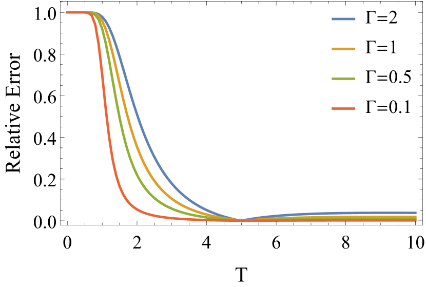
Figure 5: The relative error in the current for a noninteracting system calculated using the ME, as function of the leads’ temperature, for different coupling strengths $\Gamma$. In (a) $\varepsilon=-1$, and in (b) $\varepsilon=-10$. In both panels: $\varepsilon_{f}=0$, $V=4$, $\Gamma_{L}=\Gamma_{R}=\Gamma/2$ and $U=0$.

In Fig. 6 we plot the steady state current for the interacting system using the NEGF and its absolute value difference from the current obtained from the ME, $|I^{NEGF}-I^{ME}|$. At sufficiently high temperatures ($T\sim 10\Gamma$) the currents calculated from NEGF and the ME are in good agreement.

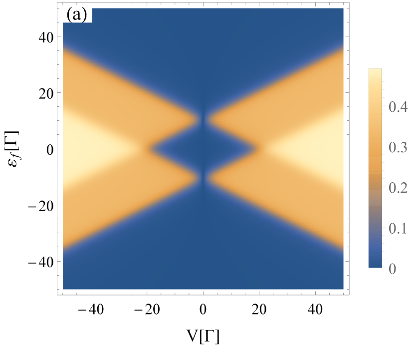
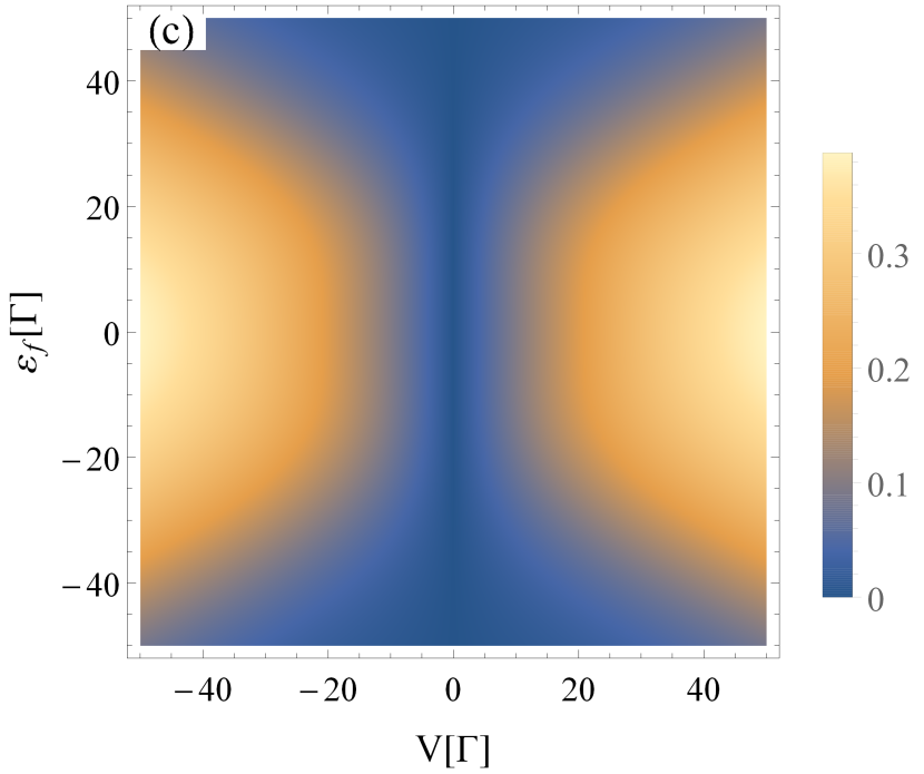
Figure 6: Left panels: the magnitude of the steady-state current in the symmetric system calculated using NEGF. Right panels: the absolute value difference between the currents calculated form NEGF and the ME. All panels are plotted as function of the Fermi-energy $\varepsilon_{f}$ and the bias voltage $V=0$. In the top panels $T_{L}=T_{R}=\Gamma$, and in the bottom $T_{L}=T_{R}=10\Gamma$. In all panels: $\varepsilon=-10\Gamma$, $U=-2\varepsilon$, and $\Gamma_{L}=\Gamma_{r}=\Gamma/2$. Note the different scales.

References

• Anderson 1961 Anderson, P. W. Localized Magnetic States in Metals. Phys. Rev. 1961, 124, 41–53
• Goldhaber-Gordon et al. 1998 Goldhaber-Gordon, D.; Shtrikman, H.; Mahalu, D.; Abusch-Magder, D.; Meirav, U.; Kastner, M. A. Kondo Effect in a Single-Electron Transistor. Nature (London) 1998, 391, 156–159
• Hanson et al. 2007 Hanson, R.; Kouwenhoven, L.; Petta, J.; Tarucha, S.; Vandersypen, L. Spins in Few-Electron Quantum Dots. Rev. Mod. Phys. 2007, 79, 1217–1265
• Nitzan and Ratner 2003 Nitzan, A.; Ratner, M. A. Electron Transport in Molecular Wire Junctions. Science 2003, 300, 1384–1389
• Heath and Ratner 2003 Heath, J. R.; Ratner, M. A. Molecular Electronics. Phys. Today 2003, 56, 43–49
• Beenakker 1991 Beenakker, C. W. J. Theory of Coulomb-Blockade Oscillations in the Conductance of a Quantum Dot. Phys. Rev. B 1991, 44, 1646–1656
• Koch et al. 2006 Koch, J.; Raikh, M. E.; Von Oppen, F. Pair Tunneling Through Single Molecules. Phys. Rev. Lett. 2006, 96, 056803
• Kondo 1964 Kondo, J. Resistance Minimum in Dilute Magnetic Alloys. Prog. Theor. Phys. 1964, 32, 37–49
• Schrieffer and Wolff 1966 Schrieffer, J. R.; Wolff, P. A. Relation Between the Anderson and Kondo Hamiltonians. Phys. Rev. 1966, 149, 491–492
• Datta 1990 Datta, S. A Simple Kinetic-Equation for Steady-State Quantum Transport. J. Phys. C 1990, 2, 8023–8052
• Harbola et al. 2006 Harbola, U.; Esposito, M.; Mukamel, S. Quantum Master Equation for Electron Transport Through Quantum Dots and Single Molecules. Phys. Rev. B 2006, 74, 235309
• Leijnse and Wegewijs 2008 Leijnse, M.; Wegewijs, M. R. Kinetic Equations for Transport Through Single-Molecule Transistors. Phys. Rev. B 2008, 78, 235424
• Esposito and Galperin 2009 Esposito, M.; Galperin, M. Transport in Molecular States Language: Generalized Quantum Master Equation Approach. Phys. Rev. B 2009, 79, 205303
• Esposito and Galperin 2010 Esposito, M.; Galperin, M. Self-Consistent Quantum Master Equation Approach to Molecular Transport. J. Phys. Chem. C 2010, 114, 20362–20369
• Dou et al. 2015 Dou, W.; Nitzan, A.; Subotnik, J. E. Surface Hopping with a Manifold of Electronic States. III. Transients, Broadening, and the Marcus Picture. J. Chem. Phys. 2015, 142, 234106
• Dorda et al. 2015 Dorda, A.; Ganahl, M.; Evertz, H. G.; Von Der Linden, W.; Arrigoni, E. Auxiliary Master Equation Approach within Matrix Product States: Spectral Properties of the Nonequilibrium Anderson Impurity Model. Phys. Rev. B 2015, 92, 125145
• Hettler et al. 1998 Hettler, M. H.; Kroha, J.; Hershfield, S. Nonequilibrium Dynamics of the Anderson Impurity Model. Phys. Rev. B 1998, 58, 5649–5664
• Datta 2000 Datta, S. Nanoscale Device Modeling: the Green’s Function Method. Superlattices and Microstructures 2000, 28, 253–278
• Xue et al. 2002 Xue, Y. Q.; Datta, S.; Ratner, M. A. First-Principles Based Matrix Green’s Function Approach to Molecular Electronic Devices: General Formalism. Chem. Phys. 2002, 281, 151–170
• Galperin et al. 2007 Galperin, M.; Ratner, M. A.; Nitzan, A. Molecular Transport Junctions: Vibrational Effects. J. Phys.: Condens. Matter 2007, 19, 103201
• Galperin et al. 2007 Galperin, M.; Nitzan, A.; Ratner, M. A. Inelastic Effects in Molecular Junctions in the Coulomb and Kondo Regimes: Nonequilibrium Equation-of-Motion Approach. Phys. Rev. B 2007, 76, 035301
• Haug and Jauho 2008 Haug, H.; Jauho, A.-P. Quantum Kinetics in Transport and Optics of Semiconductors, 2nd ed.; Springer series in solid-state sciences,; Springer: Berlin ; New York, 2008
• Chen et al. 2017 Chen, F.; Gao, Y.; Galperin, M. Molecular Heat Engines: Quantum Coherence Effects. Entropy 2017, 19, 472
• Stefanucci and Leeuwen 2013 Stefanucci, G.; Leeuwen, R. v. Nonequilibrium Many-Body Theory of Quantum Systems: A Modern Introduction; Cambridge University Press, 2013
• Li et al. 2013 Li, B.; Levy, T. J.; Swenson, D. W.; Rabani, E.; Miller, W. H. A Cartesian Quasi-Classical Model to Nonequilibrium Quantum Transport: The Anderson Impurity Model. J. Chem. Phys. 2013, 138, 104110
• Li et al. 2014 Li, B.; Miller, W. H.; Levy, T. J.; Rabani, E. Classical Mapping for Hubbard Operators: Application to the Double-Anderson Model. J. Chem. Phys. 2014, 140, 204106
• Mühlbacher and Rabani 2008 Mühlbacher, L.; Rabani, E. Real-Time Path Integral Approach to Nonequilibrium Many-Body Quantum Systems. Phys. Rev. Lett. 2008, 100, 176403
• Weiss et al. 2008 Weiss, S.; Eckel, J.; Thorwart, M.; Egger, R. Iterative Real-Time Path Integral Approach to Nonequilibrium Quantum Transport. Phys. Rev. B 2008, 77, 195316
• Schiró and Fabrizio 2009 Schiró, M.; Fabrizio, M. Real-Time Diagrammatic Monte Carlo for Nonequilibrium Quantum Transport. Phys. Rev. B 2009, 79, 153302
• Werner et al. 2009 Werner, P.; Oka, T.; Millis, A. J. Diagrammatic Monte Carlo Simulation of Nonequilibrium Systems. Phys. Rev. B 2009, 79, 035320
• Gull et al. 2010 Gull, E.; Reichman, D. R.; Millis, A. J. Bold-Line Diagrammatic Monte Carlo Method: General Formulation and Application to Expansion Around the Noncrossing Approximation. Phys. Rev. B 2010, 82, 075109
• Segal et al. 2010 Segal, D.; Millis, A. J.; Reichman, D. R. Numerically Exact Path-Integral Simulation of Nonequilibrium Quantum Transport and Dissipation. Phys. Rev. B 2010, 82, 205323
• Cohen and Rabani 2011 Cohen, G.; Rabani, E. Memory Effects in Nonequilibrium Quantum Impurity Models. Phys. Rev. B 2011, 84, 075150
• Hartle et al. 2013 Hartle, R.; Cohen, G.; Reichman, D. R.; Millis, A. J. Decoherence and Lead-Induced Interdot Coupling in Nonequilibrium Electron Transport Through Interacting Quantum Dots: A Hierarchical Quantum Master Equation Approach. Phys. Rev. B 2013, 88, 235426
• Cohen et al. 2015 Cohen, G.; Gull, E.; Reichman, D. R.; Millis, A. J. Taming the Dynamical Sign Problem in Real-Time Evolution of Quantum Many-Body Problems. Phys. Rev. Lett. 2015, 115, 266802
• Schmitteckert 2004 Schmitteckert, P. Nonequilibrium Electron Transport Using the Density Matrix Renormalization Group Method. Phys. Rev. B 2004, 70, 121302
• Anders and Schiller 2005 Anders, F. B.; Schiller, A. Real-Time Dynamics in Quantum-Impurity Systems: A Time-Dependent Numerical Renormalization-Group Approach. Phys. Rev. Lett. 2005, 95, 196801
• Bulla et al. 2008 Bulla, R.; Costi, T. A.; Pruschke, T. Numerical Renormalization Group Method for Quantum Impurity Systems. Rev. Mod. Phys. 2008, 80, 395
• Wang and Thoss 2009 Wang, H.; Thoss, M. Numerically Exact Quantum Dynamics for Indistinguishable Particles: The Multilayer Multiconfiguration Time-Dependent Hartree Theory in Second Quantization Representation. J. Chem. Phys. 2009, 131, 024114
• Hofstetter and Kehrein 1999 Hofstetter, W.; Kehrein, S. Symmetric Anderson Impurity Model with a Narrow Band. Phys. Rev. B 1999, 59, R12732
• Dickens and Logan 2001 Dickens, N. L.; Logan, D. E. On the Scaling Spectrum of the Anderson Impurity Model. J. Phys.: Condens. Matter 2001, 13, 4505
• Motahari et al. 2016 Motahari, S.; Requist, R.; Jacob, D. Kondo Physics of the Anderson Impurity Model by Distributional Exact Diagonalization. Phys. Rev. B 2016, 94, 235133
• Schwinger 1961 Schwinger, J. Brownian Motion of a Quantum Oscillator. J. Math. Phys. 1961, 2, 407–432
• Keldysh 1964 Keldysh, L. V. Diagram Technique for Nonequilibrium Processes. Zh. Eksp. Teor. Fiz. 1964, 47, 1018
• H.-P. Breuer and F. Petruccione 2002 H.-P. Breuer and F. Petruccione, Open Quantum Systems; Oxford Univ. Press, 2002
• Nitzan 2006 Nitzan, A. Chemical Dynamics in Condensed Phases: Relaxation, Transfer, and Reactions in Condensed Molecular Systems; Oxford Univ. Press, 2006
• Ryndyk and Cuniberti 2007 Ryndyk, B. S. D. A.; Cuniberti, G. Molecular Junctions in the Coulomb Blockade Regime: Rectification and Nesting. Phys. Rev. B 2007, 76, 045408
• Scheck 2013 Scheck, F. Quantum Physics edn. 2; Springer-Verlag Berlin Heidelberg, 2013
• Levy and Rabani 2013 Levy, T. J.; Rabani, E. Symmetry Breaking and Restoration Using the Equation-of-Motion Technique for Nonequilibrium Quantum Impurity Models. J. Phys.: Condens. Matter 2013, 25, 115302
• Levy and Rabani 2013 Levy, T. J.; Rabani, E. Steady State Conductance in a Double Quantum Dot Array: The Nonequilibrium Equation-of-Motion Green Function Approach. J. Chem. Phys. 2013, 138, 164125
• Stefanucci et al. 2006 Stefanucci, G.; Almbladh, C.-O.; Kurth, S.; Gross, E. K. U.; Rubio, A.; van Leeuwen, R.; Dahlen, N. E.; von Barth, U. In Time-Dependent Density Functional Theory; Marques, M., Ullrich, C., Nogueira, F., Rubio, A., Burke, K., Gross, E., Eds.; Lecture Notes in Physics; Springer: Berlin, 2006; Vol. 706; p 479
• Devreese and van Doren 1976 Devreese, J. T., van Doren, V. E., Eds. Linear and Non-Linear Electron Transport in Solids; Nato Science Series B; 17; Plenum: New York, 1976
• Meir and Wingreen 1992 Meir, Y.; Wingreen, N. S. Landauer Formula for the Current Through an Interacting Electron Region. Phys. Rev. Lett. 1992, 68, 2512–2515
• Zubarev 1960 Zubarev, D. N. Double-time Green Functions in Statistical Physics. Sov. Phys. Usp. 1960, 320–345
• Bonch-Bruevich and Tiablikov 1962 Bonch-Bruevich, V. L.; Tiablikov, S. V. The Green Function Method in Statistical Mechanics; North-Holland Pub. Co.; Interscience Publishers Amsterdam, New York, 1962; p 251 p.