Static general relativistic solutions supported by phantom and ordinary scalar fields with higher-order potentials

Abstract

Domain wall, wormhole, particlelike, and cosmic string general relativistic solutions supported by two interacting phantom or ordinary scalar fields with 4th-, 6th-, and 8th-order potentials are studied. Numerical calculations indicate that regular finite energy solutions exist only for specific values of two free parameters of the potentials. By solving nonlinear eigenvalue problems for some fixed sets of values of the free parameters and of boundary conditions, it is shown that the presence or absence of the solutions depends on a particular symmetry of the problem, on the type of the scalar fields (ordinary or phantom), and on the form of the potential.

I Introduction

In recent years interest in obtaining solutions with various scalar fields has grown considerably, primarily because of the discovery of the accelerated expansion of the present Universe. It is now widely believed that such acceleration is caused by the presence of a special form of matter – dark energy, whose key feature is that it violates various energy conditions.

In the most extreme case, the violation of the so-called null energy condition can occur. In hydrodynamical language, this corresponds to the fact that the effective pressure of matter filling the Universe, $p$, is negative, and its modulus is greater than the energy density $\varepsilon$, i.e. $p<-\varepsilon$. Such a substance is referred to as exotic matter. As a model of exotic matter, one can consider phantom (or ghost) scalar fields, i.e., fields with the opposite sign in front of the kinetic term of the scalar field Lagrangian density. Such fields are widely used both in describing the current accelerated expansion of the Universe AmenTsu2010 and in modelling various localized objects (see below). The possible existence of phantom scalar fields in nature is indirectly supported by the observed accelerated expansion of the present Universe (see, e.g., Refs. Sullivan:2011kv ; Ade:2015xua , from which one may conclude that to explain the recent observational data one should take exotic matter into consideration).

In the present paper we consider regular solutions to Einstein’s gravitational equations supported by two ordinary or phantom scalar fields. In Ref. Dzhunushaliev:2016 , we have obtained plane symmetric (domain walls), spherically symmetric (wormholes and phantom balls), and cylindrically symmetric (cosmic strings) solutions supported by two interacting phantom scalar fields with a 4th-order potential. Here we extend those results and study the possibility of obtaining such solutions with 6th- and 8th-order potential terms. Also, we compare the obtained results with those found earlier for the 4th-order potential of Ref. Dzhunushaliev:2016 .

The aforementioned configurations are well known in the bulk of literature. Cosmic strings are extended objects that could be formed in the early Universe under phase transitions associated with spontaneous symmetry breaking Vilen ; Bran2 . In their modelling various types of scalar fields are employed Baze ; Sant , including two interacting scalar fields BezerradeMello:2003ei ; Dzhunushaliev:2007cs .

Another category of extended objects are plane symmetric domain walls, which are topological defects that arise in both particle physics and cosmology Bran2 ; Cvet . In particular, domain wall solutions may exist in theories where a scalar field potential has isolated minima, and a domain wall is a surface that separates those minima thin_dom . In such a case a scalar field changes over space and tends asymptotically to two different minima. The region where the scalar field changes rapidly corresponds to the domain wall. In the thin-wall approximation, the change in the scalar field energy density is localized on the surface of the domain wall, and it is replaced by a delta function thick_dom . In the case where all fields are constant on each side of the wall, i.e., when they are at the potential minimum, the domain walls are called vacuum domain walls.

Finally, one can consider a situation where scalar fields are localized on relatively small scales comparable to the sizes of stars. In this case, they may create spherically symmetric configurations possessing both trivial and nontrivial spacetime topologies. As an example of systems with a trivial topology, one can consider boson stars consisting of various ordinary scalar fields Schunck:2003kk ; Liebling:2012fv . In turn, the use of phantom scalar fields permits obtaining solutions of the Einstein-matter equations describing configurations both with a trivial Dzhunushaliev:2008bq and a nontrivial wormholelike topology (for a recent review on the subject, see, e.g., Ref. Bronnikov:2018vbs ), including configurations supported by complex ghost scalar fields Dzhunushaliev:2017syc .

In this paper, we consider all four types of configurations (domain walls, particlelike systems, wormholes, and cosmic strings) constructed from two interacting phantom or ordinary scalar fields with higher-order potentials. Systems with two ordinary scalar fields are well known from quantum field theory rajaraman . In the presence of a gravitational field, such systems were also repeatedly considered in the cosmological and astrophysical contexts 2_fields_syst . In our previous papers we have obtained a number of solutions with two scalar fields (both ordinary and phantom ones) which can be used both in describing astrophysical objects and when considering cosmological problems: regular spherically and cylindrically symmetric solutions 2_fields_our ; Dzhunushaliev:2007cs ; Dzhunushaliev:2015sla ; cosmological solutions Dzhunushaliev:2006xh ; Folomeev:2007uw ; thick brane solutions supported by ordinary and phantom scalar fields 2_fields_brane . In the present paper we proceed with research in this direction by considering scalar fields with different potentials.

II General equations

We consider compact gravitating configurations consisting of two real scalar fields $\phi$ and $\chi$. The modeling is carried out within the framework of Einstein’s general relativity. The corresponding Lagrangian of the system is (hereafter, we work in units where $c=\hbar=1$)

$$L=-\frac{R}{16\pi G}+\epsilon\left[\frac{1}{2}\partial_{\mu}\phi\partial^{\mu}\phi+\frac{1}{2}\partial_{\mu}\chi\partial^{\mu}\chi-V(\phi,\chi)\right],$$ (1)

where $R$ is the scalar curvature, $G$ – the Newtonian gravitational constant, $\mu,\nu=0,1,2,3$, and $\epsilon=+1$ or $-1$ corresponds to ordinary or phantom fields, respectively. Using this Lagrangian, the gravitational and scalar field equations can be written in the form:

$$R^{k}_{i}-\frac{1}{2}\delta^{k}_{i}R = \kappa T_{i}^{k},$$ (2)

$$\frac{1}{\sqrt{-g}}\frac{\partial}{\partial x^{i}}\left[\sqrt{-g}g^{ik}\frac{\partial(\phi,\chi)}{\partial x^{k}}\right] = -\frac{\partial V}{\partial(\phi,\chi)}~{},$$ (3)

where $\kappa=8\pi G$. In the present paper we assume that the interacting scalar fields have a potential in one of the forms:

$$V(\phi,\chi) = \frac{\lambda_{1}}{4}(\phi^{2}-m_{1}^{2})^{2}+\frac{\lambda_{2}}{4}(\chi^{2}-m_{2}^{2})^{2}+\phi^{2}\chi^{2}-V_{0},$$ (4)

$$V(\phi,\chi) = \frac{\lambda_{1}}{2}\phi^{2}(\phi^{2}-m_{1}^{2})^{2}+\frac{\lambda_{2}}{2}\chi^{4}(\chi^{2}-m_{2}^{2})^{2}+\frac{1}{2}\phi^{2}\chi^{2}-V_{0},$$ (5)

$$V(\phi,\chi) = \frac{\lambda_{1}}{4}\phi^{4}(\phi^{2}-m_{1}^{2})^{2}+\frac{\lambda_{2}}{2}\chi^{4}(\chi^{2}-m_{2}^{2})^{2}+\frac{1}{2}\phi^{2}\chi^{2}-V_{0}.$$ (6)

Here, $m_{1}$ and $m_{2}$ are some free parameters, $\lambda_{1}$ and $\lambda_{2}$ – self-interaction constants, and $V_{0}$ – a constant whose value can be chosen from the statement of the problem.

The corresponding energy-momentum tensor entering the right-hand side of Eq. (2) is

$$T_{\mu}^{\nu}=\epsilon\left\{\partial_{\mu}\phi\partial^{\nu}\phi+\partial_{\mu}\chi\partial^{\nu}\chi-\delta_{\mu}^{\nu}\left[\frac{1}{2}\partial_{\rho}\phi\partial^{\rho}\phi+\frac{1}{2}\partial_{\rho}\chi\partial^{\rho}\chi-V(\phi,\chi)\right]\right\}.$$ (7)

III Domain walls

Figure 1: Phantom domain wall: profiles of the phantom ($\epsilon=-1$) scalar fields $\phi(x),\chi(x)$, the metric function $a^{\prime}(x)/a(x)$, and the energy density $T^{0}_{0}(x)$ are shown. The curve 1 corresponds to the 4th-order potential (4), the curve 2 – to the 6th-order potential (5), the curve 3 – to the 8th-order potential (6). The labeling of the curves is also valid for all other figures presented below.

In considering plane symmetric domain walls solutions, we choose the metric in the form:

$$ds^{2}=a^{2}(x)(dt^{2}-dy^{2}-dz^{2})-dx^{2},$$ (8)

where $x,y,z$ are Cartesian coordinates. Then Eqs. (2)-(7) yield

$$3\left(\frac{a^{\prime}}{a}\right)^{2} = -\epsilon\left[-\frac{1}{2}\left(\phi^{\prime 2}+\chi^{\prime 2}\right)+V\right]~{},$$ (9)

$$\frac{a^{\prime\prime}}{a}-\left(\frac{a^{\prime}}{a}\right)^{2} = -\frac{\epsilon}{2}\left(\phi^{\prime 2}+\chi^{\prime 2}\right)~{},$$ (10)

$$\phi^{\prime\prime}+3\frac{a^{\prime}}{a}\phi^{\prime} = \phi\left[2\chi^{2}+\lambda_{1}(\phi^{2}-m_{1}^{2})\right]~{},$$ (11)

$$\chi^{\prime\prime}+3\frac{a^{\prime}}{a}\chi^{\prime} = \chi\left[2\phi^{2}+\lambda_{2}(\chi^{2}-m_{2}^{2})\right]~{},$$ (12)

where Eqs. (9) and (10) are the $\left({}_{1}^{1}\right)$ and $\left[\left({}_{0}^{0}\right)-\left({}_{1}^{1}\right)\right]$ components of the Einstein equations, respectively, and the prime denotes differentiation with respect to $x$. The results of numerical calculations for the phantom ($\epsilon=-1$) and ordinary $(\epsilon=+1)$ scalar fields are shown in Figs. 1 and 2, respectively. The corresponding eigenvalues of the parameters $m_{1,2}$ for the potentials (4)-(6) and $\epsilon=\pm 1$ are given in Table 1.

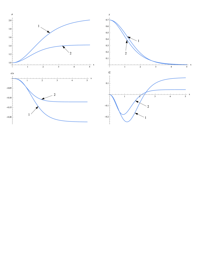
Figure 2: Ordinary domain wall: profiles of the ordinary ($\epsilon=+1$) scalar fields $\phi(x),\chi(x)$, the metric function $a^{\prime}(x)/a(x)$, and the energy density $T^{0}_{0}(x)$ are shown.

#	Potentials	$\epsilon$	$m_{1}$	$m_{2}$
1	4th-order	-1	1.77426601	1.80400455
2	6th-order	-1	1.30901092	1.73766048
3	8th-order	-1	1.4251234264	1.7965336329
4	4th-order	+1	2.05880064139	1.720175382122
5	6th-order	+1	1.42405708294	1.61615084819
6	8th-order	+1	no solution	no solution

Table 1: Eigenvalues of the parameters $m_{1},m_{2}$ for the phantom/ordinary domain wall solutions with the 4th-, 6th-, and 8th-order potentials (4)-(6). The boundary conditions at the center $x=0$ are $\phi_{0}=1,\chi_{0}=0.7,a_{0}=1,\phi^{\prime}_{0}=\chi^{\prime}_{0}=a^{\prime}_{0}=0$. The values of the free parameters $\lambda_{1}=0.15,\lambda_{2}=1.1$.

IV Phantom balls

Figure 3: Phantom ball: profiles of the scalar fields $\phi(r),\chi(r)$, the metric functions $A(r),B(r)$, and the energy density $T^{0}_{0}(r)$ are shown.

Let us now consider particlelike solutions supported by phantom fields. For this case, we choose the spherically symmetric line element in Schwarzschild coordinates

$$ds^{2}=B(r)dt^{2}-A(r)dr^{2}-r^{2}(d\theta^{2}+\sin^{2}\theta d\varphi^{2}),$$ (13)

where $r,\theta,\varphi$ are spherical coordinates. The Einstein and scalar field equations (2) and (3) together with Eq. (7) give for the phantom case

$$\frac{1}{r}\frac{A^{\prime}}{A^{2}}+\frac{1}{r^{2}}\left(1-\frac{1}{A}\right) = -\frac{1}{2A}\left(\phi^{\prime 2}+\chi^{\prime 2}\right)-V(\phi,\chi),$$ (14)

$$\frac{1}{r}\frac{B^{\prime}}{AB}-\frac{1}{r^{2}}\left(1-\frac{1}{A}\right) = -\frac{1}{2A}\left(\phi^{\prime 2}+\ \chi^{\prime 2}\right)+V(\phi,\chi),$$ (15)

$$\frac{B^{\prime\prime}}{B}-\frac{1}{2}\left(\frac{B^{\prime}}{B}\right)^{2}-\frac{1}{2}\frac{A^{\prime}}{A}\frac{B^{\prime}}{B}-\frac{1}{r}\left(\frac{A^{\prime}}{A}-\frac{B^{\prime}}{B}\right) = 2A\left[\frac{1}{2A}\left(\phi^{\prime 2}+\chi^{\prime 2}\right)+V(\phi,\chi)\right],$$ (16)

$$\phi^{\prime\prime}+\left(\frac{2}{r}+\frac{B^{\prime}}{2B}-\frac{A^{\prime}}{2A}\right)\phi^{\prime} = A\phi\left[2\chi^{2}+\lambda_{1}(\phi^{2}-m_{1}^{2})\right]~{},$$ (17)

$$\chi^{\prime\prime}+\left(\frac{2}{r}+\frac{B^{\prime}}{2B}-\frac{A^{\prime}}{2A}\right)\chi^{\prime} = A\chi\left[2\phi^{2}+\lambda_{2}(\chi^{2}-m_{2}^{2})\right]~{},$$ (18)

where the prime denotes differentiation with respect to $r$. These equations describe spherically symmetric objects that can be called phantom balls Dzhunushaliev:2016 . The results of numerical calculations are shown in Fig. 3. Notice that the solutions for the 6th- and 8th-order potentials are practically coincide. Table 2 shows the eigenvalues of the parameters $m_{1,2}$ for the potentials (4)-(6).

#	Potentials	$m_{1}$	$m_{2}$
1	4th-order	1.54248223	1.89958804
2	6th-order	1.04506272	4.1962616
3	8th-order	1.050035	4.2023521

Table 2: Eigenvalues of the parameters $m_{1},m_{2}$ for the phantom ball solutions with the 4th-, 6th-, and 8th-order potentials (4)-(6). The boundary conditions at the center $r=0$ are $\phi_{0}=1,\chi_{0}=0.7,A_{0}=1,B_{0}=1,\phi^{\prime}_{0}=\chi^{\prime}_{0}=B^{\prime}_{0}=0$. The values of the free parameters $\lambda_{1}=0.15,\lambda_{2}=1.1$.

In the case of ordinary ($\epsilon=+1$) scalar fields and for the values of the parameters $\phi_{0}=1,\chi_{0}=0.7,\lambda_{1}=0.15,\lambda_{2}=1.1$, we did not find solutions with the potentials (4)-(6).

V Wormhole solutions

Here, it is convenient to choose the metric in polar Gaussian coordinates

$$ds^{2}=B(r)dt^{2}-dr^{2}-A(r)(d\theta^{2}+\sin^{2}\theta d\varphi^{2}),$$ (19)

where $r,\theta,\varphi$ are spherical coordinates. Then one derives the following set of Einstein’s and scalar field equations describing a traversable wormhole supported by the phantom fields $\phi,\chi$:

$$\frac{A^{\prime\prime}}{A}-\frac{1}{2}\left(\frac{A^{\prime}}{A}\right)^{2}-\frac{1}{2}\frac{A^{\prime}}{A}\frac{B^{\prime}}{B} = \phi^{\prime 2}+\chi^{\prime 2}~{},$$ (20)

$$\frac{A^{\prime\prime}}{A}+\frac{1}{2}\frac{A^{\prime}}{A}\frac{B^{\prime}}{B}-\frac{1}{2}\left(\frac{A^{\prime}}{A}\right)^{2}-\frac{1}{2}\left(\frac{B^{\prime}}{B}\right)^{2}+\frac{B^{\prime\prime}}{B} = 2\left[\frac{1}{2}(\phi^{\prime 2}+\chi^{\prime 2})+V\right],$$ (21)

$$\frac{1}{4}\left(\frac{A^{\prime}}{A}\right)^{2}-\frac{1}{A}+\frac{1}{2}\frac{A^{\prime}}{A}\frac{B^{\prime}}{B} = -\frac{1}{2}(\phi^{\prime 2}+\chi^{\prime 2})+V,$$ (22)

$$\phi^{\prime\prime}+\left(\frac{A^{\prime}}{A}+\frac{1}{2}\frac{B^{\prime}}{B}\right)\phi^{\prime} = \phi\left[2\chi^{2}+\lambda_{1}(\phi^{2}-m_{1}^{2})\right],$$ (23)

$$\chi^{\prime\prime}+\left(\frac{A^{\prime}}{A}+\frac{1}{2}\frac{B^{\prime}}{B}\right)\chi^{\prime} = \chi\left[2\phi^{2}+\lambda_{2}(\chi^{2}-m_{2}^{2})\right],$$ (24)

where the prime denotes differentiation with respect to $r$. The results of numerical calculations are shown in Fig. 4 for the eigenvalues of the parameters $m_{1,2}$ given in Table 3.

Figure 4: Traversable wormhole: profiles of the phantom scalar fields $\phi(r),\chi(r)$, the metric functions $A(r),B(r)$, and the energy density $T^{0}_{0}(r)$ are shown.

#	Potentials	$m_{1}$	$m_{2}$
1	4th-order	1.82729811	1.7869422825
2	6th-order	1.32067169	1.7205753
3	8th-order	1.45731329	1.7806672

Table 3: Eigenvalues of the parameters $m_{1},m_{2}$ for the wormhole solutions with the 4th-, 6th-, and 8th-order potentials (4)-(6). The boundary conditions at the throat $r=0$ are $\phi_{0}=1,\chi_{0}=0.7,A_{0}=-1/V\left(\phi_{0},\chi_{0}\right),B_{0}=1,\phi^{\prime}_{0}=\chi^{\prime}_{0}=A^{\prime}_{0}=B^{\prime}_{0}=0$. The values of the free parameters $\lambda_{1}=0.15,\lambda_{2}=1.1$.

VI Cosmic strings

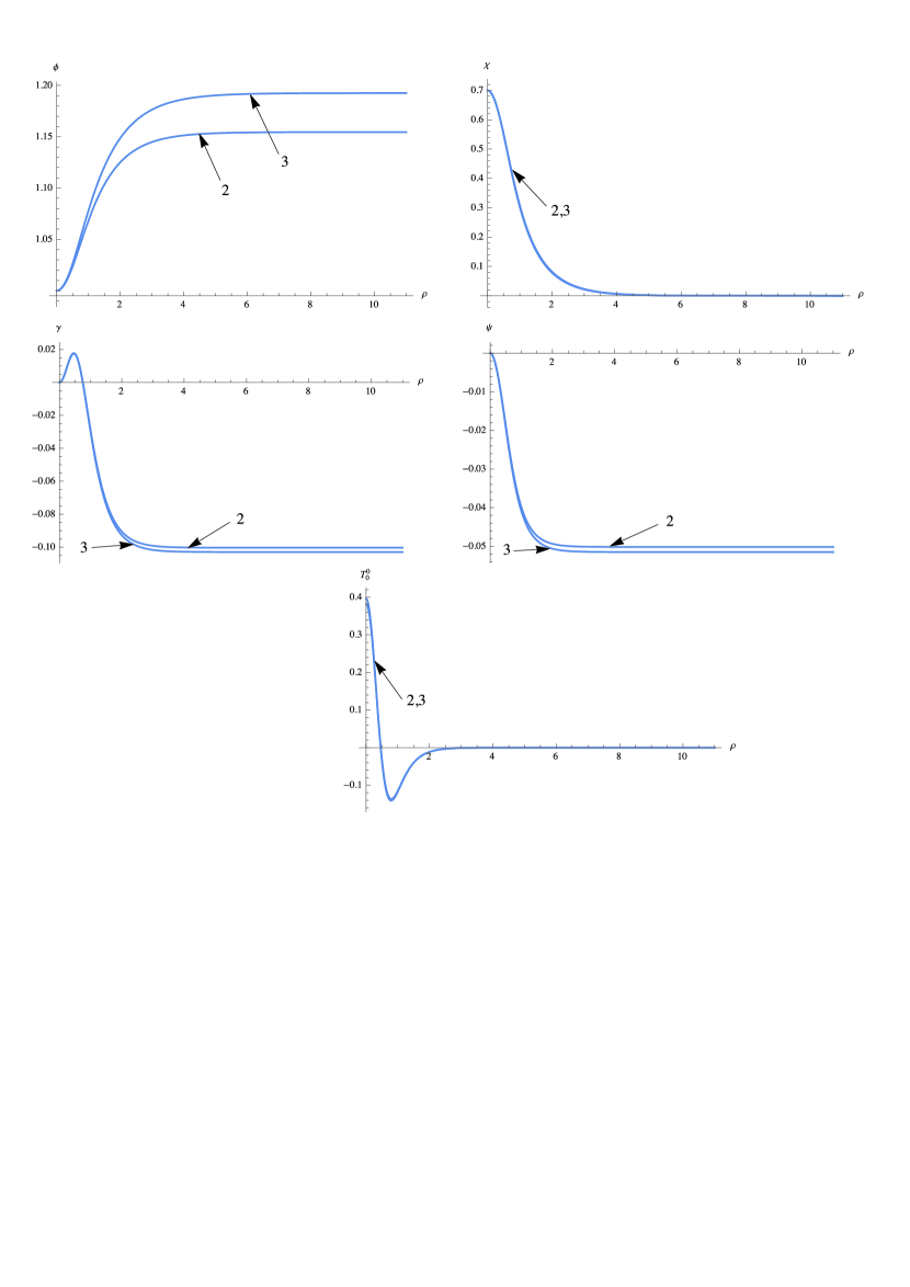
Figure 5: Phantom cosmic string: profiles of the scalar fields $\phi(\rho),\chi(\rho)$, the metric functions $\gamma(\rho),\psi(\rho)$, and the energy density $T^{0}_{0}(\rho)$ are shown.

In describing such cylindrically symmetric objects, we use the metric

$$ds^{2}=e^{2\nu(\rho)}dt^{2}-e^{2(\gamma(\rho)-\psi(\rho))}d\rho^{2}-e^{2\psi(\rho)}dz^{2}-\rho^{2}e^{-2\psi(\rho)}d\varphi^{2},$$ (25)

where $\rho,z,\varphi$ are cylindrical coordinates. In this case, one has the following Einstein and phantom scalar field equations:

$$\frac{\gamma^{\prime}}{\rho}-{\psi^{\prime}}^{2} = -\kappa\left(\frac{1}{2}{\phi^{\prime}}^{2}+\frac{1}{2}{\chi^{\prime}}^{2}+e^{2(\gamma-\psi)}V(\phi,\chi)\right),$$ (26)

$$\frac{\nu^{\prime}+\psi^{\prime}}{\rho}-{\psi^{\prime}}^{2} = -\kappa\left(\frac{1}{2}{\phi^{\prime}}^{2}+\frac{1}{2}{\chi^{\prime}}^{2}-e^{2(\gamma-\psi)}V(\phi,\chi)\right),$$ (27)

$$\psi^{\prime\prime}-\nu^{\prime\prime}-\psi^{\prime}\gamma^{\prime}+\nu^{\prime}\gamma^{\prime}-{\nu^{\prime}}^{2}+\frac{\psi^{\prime}+\gamma^{\prime}-\nu^{\prime}}{\rho} = \kappa\left(-\frac{1}{2}{\phi^{\prime}}^{2}-\frac{1}{2}{\chi^{\prime}}^{2}-e^{2(\gamma-\psi)}V(\phi,\chi)\right),$$ (28)

$$-\psi^{\prime\prime}-\nu^{\prime\prime}+\psi^{\prime}\gamma^{\prime}+\nu^{\prime}\gamma^{\prime}-2{\psi^{\prime}}^{2}-2\psi^{\prime}\nu^{\prime}-{\nu^{\prime}}^{2} = \kappa\left(-\frac{1}{2}{\phi^{\prime}}^{2}-\frac{1}{2}{\chi^{\prime}}^{2}-e^{2(\gamma-\psi)}V(\phi,\chi)\right),$$ (29)

$$\phi^{\prime\prime}+\phi^{\prime}\left(\frac{1}{\rho}-\gamma^{\prime}+\psi^{\prime}+\nu^{\prime}\right) = e^{2(\gamma-\psi)}\phi\left[2\chi^{2}+\lambda_{1}\left(\phi^{2}-m_{1}^{2}\right)\right],$$ (30)

$$\chi^{\prime\prime}+\chi^{\prime}\left(\frac{1}{\rho}-\gamma^{\prime}+\psi^{\prime}+\nu^{\prime}\right) = e^{2(\gamma-\psi)}\chi\left[2\phi^{2}+\lambda_{2}\left(\chi^{2}-m_{2}^{2}\right)\right].$$ (31)

To simplify them, let us make an additional assumption that two of the metric functions are equal, i.e., $\nu=\psi$. After some algebraic manipulations and performing the rescaling $\rho/\sqrt{\kappa}\rightarrow\rho$, $\phi\sqrt{\kappa}\rightarrow\phi$, $\chi\sqrt{\kappa}\rightarrow\chi$, and $m_{1,2}\sqrt{\kappa}\rightarrow m_{1,2}$, we get the following equations for the metric functions $\gamma(\rho),\psi(\rho)$ and the phantom $(\epsilon=-1)$ scalar fields $\phi(\rho),\chi(\rho)$:

$$\frac{\gamma^{\prime}}{\rho}-{\psi^{\prime}}^{2} = -\left(\frac{1}{2}{\phi^{\prime}}^{2}+\frac{1}{2}{\chi^{\prime}}^{2}+e^{2(\gamma-\psi)}V(\phi,\chi)\right),$$ (32)

$$2\frac{\psi^{\prime}}{\rho}-{\psi^{\prime}}^{2} = -\left(\frac{1}{2}{\phi^{\prime}}^{2}+\frac{1}{2}{\chi^{\prime}}^{2}-e^{2(\gamma-\psi)}V(\phi,\chi)\right),$$ (33)

$$\psi^{\prime\prime}+\frac{\psi^{\prime}}{\rho} = e^{2(\gamma-\psi)}\left(1-2\rho\psi^{\prime}\right)V(\phi,\chi),$$ (34)

$$\phi^{\prime\prime}+\phi^{\prime}\left(\frac{1}{\rho}-\gamma^{\prime}+2\psi^{\prime}\right) = e^{2(\gamma-\psi)}\phi\left[2\chi^{2}+\lambda_{1}\left(\phi^{2}-m_{1}^{2}\right)\right],$$ (35)

$$\chi^{\prime\prime}+\chi^{\prime}\left(\frac{1}{\rho}-\gamma^{\prime}+2\psi^{\prime}\right) = e^{2(\gamma-\psi)}\chi\left[2\phi^{2}+\lambda_{2}\left(\chi^{2}-m_{2}^{2}\right)\right],$$ (36)

where the prime denotes differentiation with respect to the rescaled radial coordinate $\rho$.

The results of numerical calculations are shown in Fig. 5 for the eigenvalues of the parameters $m_{1,2}$ given in Table 4. It is seen that the profiles for $\chi$ and for the energy densities of the 6th- and 8th-order potential cases are practically coincide.

#	Potentials	$m_{1}$	$m_{2}$
1	4th-order	no solution	no solution
2	6th-order	1.154579476	2.30250731
3	8th-order	1.1926167892	2.32316842475

Table 4: Eigenvalues of the parameters $m_{1},m_{2}$ for the phantom cosmic string solutions with the 6th- and 8th-order potentials (5) and (6). The boundary conditions at $\rho=0$ are $\phi_{0}=1,\chi_{0}=0.7,\psi_{0}=\gamma_{0}=\phi^{\prime}_{0}=\chi^{\prime}_{0}=\psi^{\prime}_{0}=0$. The values of the free parameters $\lambda_{1}=0.15,\lambda_{2}=1.1$.

In the case of ordinary ($\epsilon=+1$) scalar fields and for the values of the parameters $\phi_{0}=1,\chi_{0}=0.7,\lambda_{1}=0.15,\lambda_{2}=1.1$, we did not find solutions with the potentials (4)-(6).

Summarizing the results, we have obtained plane, cylindrically, and spherically (particlelike and wormhole) symmetric static general relativistic solutions supported by two interacting phantom/ordinary scalar fields with 4th-, 6th-, and 8th-order potentials of the form (4)-(6). All the solutions have been obtained numerically for the fixed central values of the scalar fields $\phi_{0}=1,\chi_{0}=0.7$ and for the free parameters $\lambda_{1}=0.15,\lambda_{2}=1.1$. In doing so, we have solved nonlinear eigenvalue problems for the parameters $m_{1},m_{2}$. It was shown that solutions may exist (or not exist) depending on a particular symmetry of the problem, on the type of the scalar fields (ordinary or phantom), and on the form of the potential.

References

- (1) L. Amendola and S. Tsujikawa, Dark energy: theory and observations (Cambridge University Press, Cambridge, England, 2010).
- (2) M. Sullivan et al., Astrophys. J. 737, 102 (2011).
- (3) P. A. R. Ade et al. (Planck Collaboration), Astron. Astrophys. 594, A13 (2016).
- (4) V. Dzhunushaliev, V. Folomeev, A. Makhmudov, A. Urazalina, D. Singleton and J. Scott, Phys. Rev. D 94, no. 2, 024004 (2016) [arXiv:1606.07304 [gr-qc]].
- (5) A. Vilenkin and E.P.S. Shellard, “Cosmic Strings and Other Topological Defects”, Cambridge University Press (Cambridge, 2000).
- (6) J. Magueijo and R. H. Brandenberger, “Cosmic Defects and Cosmology”, astro-ph/0002030.
- (7) D. Bazeia, H. Boschi-Filho and F. A. Brito, JHEP 9904, 028 (1999) [hep-th/9811084].
- (8) C. Santos, Class. Quant. Grav. 18, 1835 (2001) [gr-qc/0009102].
- (9) E. R. Bezerra de Mello, Y. Brihaye and B. Hartmann, Phys. Rev. D 67, 124008 (2003) [hep-th/0302212].
- (10) V. Dzhunushaliev and V. Folomeev, Int. J. Mod. Phys. D 17, 2125 (2008) [arXiv:0711.2840 [gr-qc]].
- (11) M. Cvetic and H. H. Soleng, Phys. Rept. 282, 159 (1997) [hep-th/9604090].
- (12) V.A. Berezin, V.A. Kuzmin, I.I. Tkachev, Phys.Lett. 120B, 91 (1983); V.A. Berezin, V.A. Kuzmin, I.I. Tkachev, Phys.Rev. D36, 2919 (1987); D. Garfinkle, C. Vuille, Class.Quant.Grav. 6, 1819 (1989); J.R. Ipser, P. Sikivie, Phys.Rev. D30, 712 (1984); P. Laguna-Castillo, R.A. Matzner, Phys.Rev. D34, 2913 (1986).
- (13) H. Arodz, Phys.Rev. D52, 1082 (1995); H. Arodz, A.L. Larsen, Phys.Rev. D49, 4154 (1994); G. Goetz, J.Math.Phys. 31, 2683 (1990); L.M. Widrow, Phys.Rev. D40, 1002 (1989).
- (14) F. E. Schunck and E. W. Mielke, Classical Quantum Gravity 20, R301 (2003).
- (15) S. L. Liebling and C. Palenzuela, Living Rev. Relativity 15, 6 (2012).
- (16) V. Dzhunushaliev, V. Folomeev, R. Myrzakulov, and D. Singleton, J. High Energy Phys. 07 (2008) 094.
- (17) K. A. Bronnikov, Particles 1, no. 1, 5 (2018) [arXiv:1802.00098 [gr-qc]].
- (18) V. Dzhunushaliev, V. Folomeev, B. Kleihaus and J. Kunz, Phys. Rev. D 97, no. 2, 024002 (2018) [arXiv:1710.01884 [gr-qc]].
- (19) R. Rajaraman, An Introduction to Solitons and Instantons in Quantum Field Theory (North-Holland, Amsterdam, 1982).
- (20) D. Bazeia, M. J. dos Santos and R. F. Ribeiro, Phys. Lett. A 208, 84 (1995) [arXiv:hep-th/0311265]; D. Bazeia, J. R. S. Nascimento, R. F. Ribeiro, and D. Toledo, J. Phys. A 30, 8157 (1997) [arXiv:hep-th/9705224]; D. Bazeia and A. R. Gomes, JHEP 0405, 012 (2004) [arXiv:hep-th/0403141]; S. Y. Vernov, Teor. Mat. Fiz. 155, 47 (2008) [Theor. Math. Phys. 155, 544 (2008)] [arXiv:astro-ph/0612487]; I. Y. Aref’eva, N. V. Bulatov, and S. Y. Vernov, Theor. Math. Phys. 163, 788 (2010) [arXiv:0911.5105 [hep-th]].
- (21) V. Dzhunushaliev, K. Myrzakulov, and R. Myrzakulov, Mod. Phys. Lett. A 22, 273 (2007) [arXiv:gr-qc/0604110]; V. Dzhunushaliev, V. Folomeev, K. Myrzakulov, and R. Myrzakulov, Mod. Phys. Lett. A 22, 407 (2007) [arXiv:gr-qc/0610111].
- (22) V. Dzhunushaliev, V. Folomeev and A. Urazalina, Int. J. Mod. Phys. D 24, no. 14, 1550097 (2015) [arXiv:1506.03897 [gr-qc]].
- (23) V. Dzhunushaliev, V. Folomeev, K. Myrzakulov and R. Myrzakulov, Int. J. Mod. Phys. D 17, 2351 (2008) [gr-qc/0608025].
- (24) V. Folomeev, Int. J. Mod. Phys. D 16, 1845 (2007) [gr-qc/0703004 [GR-QC]]..
- (25) V. Dzhunushaliev, Grav. Cosmol. 13, 302 (2007) [arXiv:gr-qc/0603020]; V. Dzhunushaliev, V. Folomeev, D. Singleton, and S. Aguilar-Rudametkin, Phys. Rev. D 77, 044006 (2008) [arXiv:hep-th/0703043]; V. Dzhunushaliev, V. Folomeev, K. Myrzakulov, and R. Myrzakulov, Gen. Rel. Grav. 41, 131 (2009) [arXiv:0705.4014 [gr-qc]]; V. Dzhunushaliev, V. Folomeev, and M. Minamitsuji, Phys. Rev. D 79, 024001 (2009) [arXiv:0809.4076 [gr-qc]]; V. Dzhunushaliev, V. Folomeev, and M. Minamitsuji, Rept. Prog. Phys. 73, 066901 (2010) [arXiv:0904.1775 [gr-qc]].