Low dimensional matrix representations for noncommutative surfaces of arbitrary genus

Abstract.

In this note, we initiate a study of the finite-dimensional representation theory of a class of algebras that correspond to noncommutative deformations of compact surfaces of arbitrary genus. Low dimensional representations are investigated in detail and graph representations are used in order to understand the structure of non-zero matrix elements. In particular, for arbitrary genus greater than one, we explicitly construct classes of irreducible two and three dimensional representations. The existence of representations crucially depends on the analytic structure of the polynomial defining the surface as a level set in $\mathbb{R}^{3}$.

1. Introduction

Understanding the geometry of noncommutative space is believed to be crucial in order to approach a quantum theory of gravity. Both String theory (via the IKKT model [IKKT97]) and the matrix regularization of Membrane theory [Hop82, dWHN88], being candidates for describing quantum effects in gravity, contain noncommutative (matrix) analogues of 2-dimensional manifolds. For compact surfaces, one considers sequences of matrix algebras of increasing dimension, converging (in a certain sense [Hop82, BHSS91, AHH12]) to the Poisson algebra of functions on the surface. By now, surfaces of genus zero and one are quite well understood (see e.g. [Hop82, FFZ89, Hop88, Hop89, Mad92]), but understanding the case of higher genus has turned out to be more difficult. Although there are several results that treat the case of higher genus and prove the existence of matrix algebras converging to the algebra of smooth functions (see e.g. [KL92a, KL92b, KL94, BMS94, NN99]), explicit representations, as well as an algebraic understanding of these objects, are still lacking to a large extent. Other interesting approaches to matrix regularizations have also appeared which focus slightly more on approximation properties, as well as connections to physics, and how geometry emerges from limits of matrix algebras (see e.g. [Shi04, Ste10, Syk16]).

In [ABH⁺09a, ABH⁺09b] a class of algebras, defined by generators and relations, was given as a candidate for noncommutative analogues of compact surfaces of arbitrary genus. A one-parameter family of surfaces interpolating between spheres and tori was thoroughly investigated and all finite-dimensional representations were classified. However, only marginal progress was made in understanding if the proposed relations are consistent and tractable for the higher genus case, and no concrete representations were constructed. In this note, we study low dimensional representations of these algebras for arbitrary genus greater than one. One should expect, due to the high polynomial order of the defining relations, that the representation theory is quite complicated and to better understand its structure, we shall make use of graph methods to describe non-zero matrix elements; a method which has previously turned out to be most helpful in understanding finite-dimensional representations [Arn08a, Arn08b, ABH⁺09a, ABH⁺09b, AH10]. Via these graphs, one can easily derive conditions which may be used to exclude certain matrices from being representations.

Two dimensional representations are studied in detail, and even this simple case turns out to be rather complicated, indicating what to expect in the higher dimensional case. In particular, we show that one can construct 2-dimensional representations for any genus $g\geq 2$ and any value of the deformation parameter $\hbar>0$. The existence of these representations depends crucially on the analytic structure of a polynomial defining the surface as a level set in $\mathbb{R}^{3}$.

2. Compact genus $g$ surfaces in $\mathbb{R}^{3}$ as level sets

Let us recall how a class of compact surfaces of arbitrary genus may be constructed as level sets in $\mathbb{R}^{3}$ [Hof07, ABH⁺09a, ABH⁺09b]. Let $g\geq 1$ be an integer and set

$$G(t)=\prod_{k=1}^{g}(t-k^{2})\qquad M=\!\!\!\!\max_{0\leq t\leq g^{2}+1}\!\!\!G(t).$$

For arbitrary $c>0$ and $\alpha\in(0,2\sqrt{c}/M)$ set

$$p(x)=\alpha G(x^{2})-\sqrt{c}=\alpha\prod_{k=1}^{g}(x^{2}-k^{2})-\sqrt{c}$$

and

$$C(x,y,z)=\frac{1}{2}\big{(}p(x)+y^{2}\big{)}^{2}+\frac{1}{2}z^{2}-\frac{1}{2}c.$$

Using Morse theory is is straightforward to show that the level set $\Sigma_{g}=C^{-1}(0)$ is a compact surface of genus $g$. An example of a surface of genus 3 is given in Figure 1. In the next section, we shall start by investigating some of the properties of the polynomial $p(x)$, which will later become important when proving existence of representations.

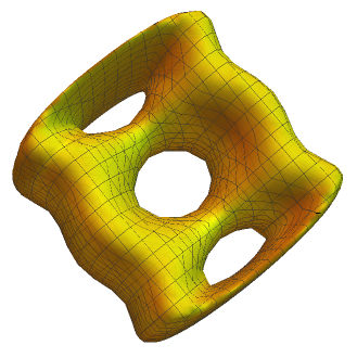
Figure 1. An example of $\Sigma_{3}$ as a level set in $\mathbb{R}^{3}$.

2.1. Properties of $p(x)$

First of all, one notes that

$$p(k)=-\sqrt{c}<0$$

for $k=1,2,\ldots,g$ and

$$p^{\prime}(x)=2\alpha x\sum_{k=1}^{g}\prod_{l=1,l\neq k}^{g}(x^{2}-l^{2})$$

giving

(2.1) $$p^{\prime}(k)=2\alpha k\prod_{l=1,l\neq k}^{g}(k^{2}-l^{2})=(-1)^{g-k}\,\frac{\alpha(g+k)!(g-k)!}{k}$$

for $k=1,2,\ldots,g$. Furthermore, $p(-x)=x$ and $p^{\prime}(-x)=-p^{\prime}(x)$. As an illustration of the typical behavior of the polynomial, a plot of $p(x)$ can be found in Figure 2.

Figure 2. Plot of the polynomial $p(x)$ for $g=4$ ($c=1$ and $\alpha=1/1664$).

In the next result we give two simple, but useful, lower bounds of the maximum of $G(t)$ in the interval $0\leq t\leq g^{2}+1$.

Lemma 2.1.

If

$$G(t)=\prod_{k=1}^{g}(t-k^{2})\quad\text{and}\quad M=\!\!\!\!\max_{0\leq t\leq g^{2}+1}\!\!\!G(t)$$

then $M\geq(2g-1)!/g$ and $M\geq(g!)^{2}$.

Proof.

First we note that

$$M \geq G(g^{2}+1)=\prod_{k=1}^{g}(g^{2}+1-k^{2})\geq\prod_{k=1}^{g-1}(g^{2}-k^{2})=\prod_{k=1}^{g-1}(g+k)(g-k)$$

$$=\frac{(2g-1)!}{g},$$

proving the first inequality. Next, for $g\leq 4$ one verifies that

$$g=1:\qquad M\geq G(g^{2}+1)=1=(1!)^{2}$$

$$g=2:\qquad M\geq G(g^{2}+1)=4=(2!)^{2}$$

$$g=3:\qquad M\geq G(g^{2}+1)=54>36=(3!)^{2}$$

$$g=4:\qquad M\geq G(g^{2}+1)=1664>576=(4!)^{2}.$$

Now, assume $g\geq 5$ and write

$$M-(g!)^{2} \geq\frac{(2g-1)!}{g}-(g!)^{2}$$

$$=(g-1)!\Big{(}(g+1)(g+2)\cdots(2g-1)-g\cdot g(g-1)\cdots 2\cdot 1\Big{)}$$

$$=(g-1)!\Big{(}(g+1)(g+2)\cdots(2g-1)-g\cdot g(g-1)\cdots 5\cdot 4\cdot 6\Big{)}.$$

As written, each product inside the parenthesis has $g-1$ factors, and every factor in the positive term is $\geq g+1$ and every factor in the negative term is $\leq g+1$ (since $g\geq 5$). Thus, we conclude that $M-(g!)^{2}\geq 0$. ∎

With the help of the above lemma, one can prove the following result.

Lemma 2.2.

For $\alpha\in(0,2\sqrt{c}/M)$ it holds that

$$p(0)+3\sqrt{c}>0\quad\text{and}\quad p(0)-\sqrt{c}<0.$$

Proof.

The two inequalities can be written as

$$(-1)^{g}\alpha(g!)^{2}+2\sqrt{c}>0$$

$$(-1)^{g}\alpha(g!)^{2}-2\sqrt{c}<0,$$

and they are trivially satisfied if $g$ is even and odd, respectively. In the opposite case, these inequalities are both equivalent to

$$\alpha(g!)^{2}<2\sqrt{c}\quad\Leftrightarrow\quad\frac{\alpha}{\sqrt{c}}<\frac{2}{(g!)^{2}}.$$

Recalling that $\alpha<2\sqrt{c}/M$, Lemma 2.1 implies that

$$\frac{\alpha}{\sqrt{c}}<\frac{2}{M}\leq\frac{2}{(g!)^{2}}$$

yielding the desired result. ∎

3. Noncommutative surfaces of arbitrary genus

In this section we will recall a class of noncommutative algebras corresponding to deformations of algebras of smooth functions on the level sets $\Sigma_{g}=C^{-1}(0)$. For arbitrary $C\in C^{\infty}(\mathbb{R}^{3})$ the relation

$$\{x^{i},x^{j}\}=\varepsilon^{ijk}(\partial_{k}C)$$

(with $x^{1}=x$, $x^{2}=y$, $x^{3}=z$) defines a Poisson structure on $C^{\infty}(\mathbb{R}^{3})$ that restricts to the level set $C(x,y,z)=0$. For the particular case when

$$C(x,y,z)=\frac{1}{2}\big{(}p(x)+y^{2}\big{)}^{2}+\frac{1}{2}z^{2}-\frac{1}{2}c$$

one obtains

$$\{x,y\}=z$$

$$\{y,z\}=p(x)p^{\prime}(x)+y^{2}p^{\prime}(x)$$

$$\{z,x\}=2y^{3}+2yp(x).$$

In order to find noncommutative deformations of the above Poisson algebra, one replaces $\{\cdot,\cdot\}$ by $[\cdot,\cdot]/(i\hbar)$ and considers the relations (cf. [ABH⁺09b])

(3.1) $$[X,Y]=i\hbar Z$$

(3.2) $$[Y,Z]=i\hbar\big{(}p(X)p^{\prime}(X)+\mathcal{T}(X,Y^{2})\big{)}$$

(3.3) $$[Z,X]=i\hbar\big{(}2Y^{3}+Yp(X)+p(X)Y\big{)}$$

where $\mathcal{T}(X,Y^{2})$ denotes a noncommutative polynomial such that its commutative image $\mathcal{T}(x,y^{2})$ equals $p^{\prime}(x)y^{2}$; for instance

$$\mathcal{T}\big{(}X,Y^{2}\big{)}=\tfrac{1}{2}Y^{2}p^{\prime}(X)+\tfrac{1}{2}p^{\prime}(X)Y^{2}.$$

In other words, $\mathcal{T}$ represents a choice of noncommutative ordering of the product of $y^{2}$ and $p^{\prime}(x)$. Let us keep this choice arbitrary for the moment and define the noncommutative algebra that will be of interest for us.

Definition 3.1.

For $g\geq 1$, $c>0$, $\alpha\in(0,2\sqrt{c}/M)$ and $\hbar>0$, let $I_{\hbar}^{g}(\alpha,c)$ denote the two-sided ideal, in the (unital) free $\ast$-algebra $\mathbb{C}\left\langle X,Y,Z\right\rangle$ (with $X,Y,Z$ hermitian), generated by (3.1)–(3.3). We set

$$\mathcal{C}_{\hbar}^{g}(\alpha,c)=\mathbb{C}\left\langle X,Y,Z\right\rangle/I_{\hbar}^{g}(\alpha,c).$$

Remark 3.2.

Note that we shall often simply write $\mathcal{C}_{\hbar}^{g}$ and tacitly assume an arbitrary choice of $\alpha$ and $c$ such that $\alpha\in(0,2\sqrt{c}/M)$.

For fixed genus $g$, the algebra $\mathcal{C}_{\hbar}^{g}(\alpha,c)$ is defined by the three parameters $\hbar,\alpha,c$. However, algebras defined by distinct parameters might be isomorphic, as shown in the next result.

Proposition 3.3.

If $\mathcal{C}^{g}_{\hbar_{1}}(\alpha_{1},c_{1})$ and $\mathcal{C}^{g}_{\hbar_{2}}(\alpha_{2},c_{2})$ are algebras such that

$$\frac{\alpha_{1}}{\sqrt{c_{1}}}=\frac{\alpha_{2}}{\sqrt{c_{2}}}\quad\text{and}\quad\hbar_{2}=\hbar_{1}\sqrt{\frac{\alpha_{1}}{\alpha_{2}}},$$

then $\mathcal{C}^{g}_{\hbar_{1}}(\alpha_{1},c_{1})\simeq\mathcal{C}^{g}_{\hbar_{2}}(\alpha_{2},c_{2})$.

Proof.

Let $\lambda=\sqrt{\alpha_{1}}/\sqrt{\alpha_{2}}$ giving $\hbar_{2}=\lambda\hbar_{1}$. We shall prove that

$$\varphi(X_{1})=X_{2}\qquad\varphi(Y_{1})=\lambda Y_{2}\qquad\varphi(Z_{1})=\lambda^{2}Z_{2}$$

defines an isomorphism $\varphi:\mathcal{C}^{g}_{\hbar_{1}}(\alpha_{1},c_{1})\to\mathcal{C}^{g}_{\hbar_{2}}(\alpha_{2},c_{2})$. It is clear that $\varphi$ is invertible, but to show that it is an algebra homomorphism, one needs to prove that it respects the relations defining $I_{\hbar}^{g}$. First of all, we find that

$$[\varphi(X_{1}),\varphi(Y_{1})]-i\hbar_{1}\varphi(Z_{1})=\lambda[X_{2},Y_{2}]-i\hbar_{1}\lambda^{2}Z_{2}=i\lambda\hbar_{2}Z_{2}-i\lambda\hbar_{2}Z_{2}=0.$$

Recalling that

$$p_{i}(x)=\alpha_{i}\prod_{k=1}^{g}(x^{2}-k^{2})-\sqrt{c_{i}}\qquad(i=1,2)$$

together with $\alpha_{1}=\lambda^{2}\alpha_{2}$ and $\sqrt{c_{1}}=\lambda^{2}\sqrt{c_{2}}$, we find that

$$p_{1}(x)=\lambda^{2}p_{2}(x)\quad\text{and}\quad p_{1}^{\prime}(x)=\lambda^{2}p^{\prime}_{2}(x).$$

Now, one can show that

$$[\varphi(Y_{1}),\varphi(Z_{1})]-i\hbar_{1}p_{1}\big{(}\varphi(X_{1})\big{)}p_{1}^{\prime}\big{(}\varphi(X_{1})\big{)}-i\hbar_{1}\mathcal{T}_{1}\big{(}\varphi(X_{1}),\varphi(Y_{1})^{2}\big{)}$$

$$\qquad=\lambda^{3}[Y_{2},Z_{2}]-i\hbar_{1}\lambda^{4}p_{2}(X_{2})p_{2}^{\prime}(X_{2})-i\hbar_{1}\lambda^{4}\mathcal{T}_{2}(X_{2},Y_{2}^{2})$$

$$\qquad=\lambda^{3}[Y_{2},Z_{2}]-i\hbar_{2}\lambda^{3}p_{2}(X_{2})p_{2}^{\prime}(X_{2})-i\hbar_{2}\lambda^{3}\mathcal{T}_{2}(X_{2},Y_{2}^{2})=0,$$

as well as

$$[\varphi(Z_{1}), \varphi(X_{1})]-2i\hbar_{1}\varphi(Y_{1})^{3}-i\hbar_{1}\varphi(Y_{1})p_{1}(\varphi(X_{1}))-i\hbar_{1}p_{1}(\varphi(X_{1}))\varphi(Y_{1})$$

$$=\lambda^{2}[Z_{2},X_{2}]-2i\hbar_{1}\lambda^{3}Y_{1}p_{2}(X_{2})-i\hbar_{1}\lambda^{3}p_{2}(X_{2})Y_{2}$$

$$=\lambda^{2}[Z_{2},X_{2}]-2i\hbar_{2}\lambda^{2}Y_{2}p_{2}(X_{2})-i\hbar_{2}\lambda^{2}p_{2}(X_{2})Y_{2}=0.$$

This proves that $\varphi$ is indeed an algebra homomorphism. ∎

Thus, up to a rescaling of the deformation parameter $\hbar$, the quotient $\alpha/\sqrt{c}$ is the essential parameter of the algebra $\mathcal{C}_{\hbar}^{g}$. This may come as no surprise, since it is the same quotient that determines the location of the roots of $p(x)$.

In [ABH⁺09a, ABH⁺09b] the analogous algebra for the choice

$$C(x,y,z)=\frac{1}{2}(x^{2}+y^{2}-\mu)^{2}+\frac{1}{2}z^{2}-\frac{1}{2}c$$

was investigated in detail. For $-\sqrt{c}<\mu<\sqrt{c}$ the inverse image has genus 0, and for $\mu>\sqrt{c}$ the inverse image has genus 1, allowing one to study topology transition by varying the parameter $\mu$. It turns out that one can classify all finite-dimensional (hermitian) representations in terms of directed graphs. Curiously, the structure of the graph clearly reflects the topology of the surface with “strings” representing genus 0 and “cycles” representing genus 1. It is an interesting question whether or not a similar statement is true in the higher genus case.

4. Representations of $\mathcal{C}_{\hbar}^{g}$

We aim to construct representations $\phi:\mathcal{C}_{\hbar}^{g}\to\operatorname{Mat}(n,\mathbb{C})$ such that $\phi(X)$, $\phi(Y)$ and $\phi(Z)$ are hermitian matrices. When it is clear from the context, we shall for convenience simply write $X,Y,Z$ instead of $\phi(X),\phi(Y),\phi(Z)$. Note that since the matrix algebra generated by a representation is invariant under hermitian conjugation, every reducible representation will be completely reducible.

By applying a unitary transformation, one may assume that $X$ is diagonal with

$$X=\operatorname{diag}(x_{1},x_{2},\ldots,x_{n})\qquad x_{i}\in\mathbb{R},$$

and we note that $Z$ can be eliminated from (3.1)–(3.3) (as $Z=\tfrac{1}{i\hbar}[X,Y]$) giving

(4.1) $$\big{[}[X,Y],Y\big{]}=\hbar^{2}\big{(}p(X)p^{\prime}(X)+\mathcal{T}(X,Y^{2})\big{)}$$

(4.2) $$\big{[}[Y,X],X\big{]}=\hbar^{2}\big{(}2Y^{3}+Yp(X)+p(X)Y\big{)}.$$

Up to now, the choice of $\mathcal{T}(X,Y^{2})$ has been quite arbitrary, and it is time to introduce a few assumptions as well as develop some notation in the case when $X$ is diagonal. Namely, for an arbitrary choice of $\mathcal{T}$, every term will be of the form $X^{k}Y^{2}X^{l}$ for some $k,l\geq 0$. If $X$ is assumed to be diagonal, this implies that there exists a polynomial $\hat{p}(x,y)$ such that

$$\mathcal{T}(X,Y^{2})_{ij}=\hat{p}(x_{i},x_{j})\sum_{k=1}^{n}y_{ik}y_{kj},$$

giving $\hat{p}(x,x)=p^{\prime}(x)$. For instance, if $\mathcal{T}=(p^{\prime}(X)Y^{2}+Y^{2}p^{\prime}(X))/2$ then

(4.3) $$\hat{p}(x,y)=\frac{1}{2}\big{(}p^{\prime}(x)+p^{\prime}(y)\big{)}.$$

In the following, we shall assume that $\mathcal{T}$ is chosen such that

$$\hat{p}(x,y)=\hat{p}(y,x)\quad\text{and}\quad\hat{p}(x,-x)=0,$$

which is clearly true for (4.3) since $p^{\prime}(-x)=-p^{\prime}(x)$.

The $(i,j)$ matrix elements of (4.1) and (4.2) can then be written as

(A_ij) $$\sum_{k=1}^{n}\big{(}q_{\hbar}(x_{i},x_{j})-2x_{k}\big{)}y_{ik}y_{kj}=\hbar^{2}\delta_{ij}p(x_{i})p^{\prime}(x_{j})$$

(B_ij) $$2h^{2}\sum_{k,l=1}^{n}y_{ik}y_{kl}y_{lj}=r_{\hbar}(x_{i},x_{j})y_{ij}$$

where

$$q_{\hbar}(x,y)=x+y-\hbar^{2}\hat{p}(x,y)$$

$$r_{\hbar}(x,y)=(x-y)^{2}-\hbar^{2}\big{(}p(x)+p(y)\big{)}.$$

We note that $q_{\hbar}(x,y)=q_{\hbar}(y,x)$ and $r_{\hbar}(x,y)=r_{\hbar}(y,x)$ as well as

$$q_{\hbar}(x,x)=2x-\hbar^{2}p^{\prime}(x) q_{\hbar}(x,-x)=0$$

$$r_{\hbar}(x,x)=-2\hbar^{2}p(x) r_{\hbar}(x,-x)=4x^{2}-2\hbar^{2}p(x).$$

Since $Y$ is hermitian equation A_ij is equivalent to A_ji (due to $q_{\hbar}$ being symmetric) and equation B_ij is equivalent to B_ji; therefore, it is sufficient to consider A_ij and B_ij for $i\leq j$. In particular, for $i=j$ one gets

(A_ii) $$\sum_{k=1}^{n}\big{(}2(x_{i}-x_{k})-\hbar^{2}p^{\prime}(x_{i})\big{)}|y_{ik}|^{2}=\hbar^{2}p(x_{i})p^{\prime}(x_{i}).$$

For a matrix regularization, the matrices $X$, $Y$ and $Z$ correspond to the the functions $x$, $y$ and $z$, respectively, and representations with $\phi(Z)=0$ might be considered degenerate from this point of view. Therefore, we make the following definition.

Definition 4.1.

A representation $\phi$ of $\mathcal{C}_{\hbar}^{g}$ is called degenerate if $\phi(Z)=0$. If a representation is not degenerate, it is called non-degenerate.

It immediately follows that the structure of degenerate representations is simple.

Proposition 4.2.

A degenerate representation of $\mathcal{C}_{\hbar}^{g}$ is completely reducible to a sum of 1-dimensional representations.

Proof.

Let $X,Y,Z$ be hermitian matrices of a representation of $\mathcal{C}_{\hbar}^{g}$. Assuming that $Z=0$ it follows that $0=i\hbar Z=[X,Y]$ and since $X$ and $Y$ are hermitian, there exists a basis where they are both diagonal. Thus, every matrix in the representation is diagonal and hence equivalent to a direct sum of 1-dimensional representations. ∎

4.1. The directed graph of $Y$

Constructing representations of $\mathcal{C}_{\hbar}^{g}$, in a basis where $X$ is diagonal, is equivalent to solving equations (A_ij) and (B_ij) for the matrix elements of $X$ and $Y$. In doing so, it is convenient to encode the structure of the non-zero matrix elements of $Y$ in a graph. Therefore, let us recall the concept of a graph associated to a matrix.

Definition 4.3.

Let $Y$ be a hermitian $(n\times n)$-matrix with matrix elements $y_{ij}$ for $i,j\in\{1,\ldots,n\}$. The graph of $Y$ is the (undirected) graph $G=(V,E)$ on $n$ vertices such that $(ij)\in E$ if and only if $y_{ij}\neq 0$.

Note that the above definition implies that a graph may have self-loops, i.e. $(ii)\in E$. To distinguish between such a graph, and a graph without self-loops, we shall refer to the latter as a simple graph. Furthermore, by a walk we mean a sequence of vertices $(i_{1}i_{2}\cdots i_{N})$ such that $(i_{k}i_{k+1})\in E$ for $1\leq k\leq N-1$. A path is a walk $(i_{1}i_{2}\cdots i_{N})$ such that $i_{k}\neq i_{l}$ if $k\neq l$. The length of a walk $(i_{1}i_{2}\cdots i_{N})$ is $N-1$. For a connected graph G, we let $d(i,j)$ denote the length of the shortest walk starting at $i\in V$ and ending at $j\in V$.

Definition 4.4.

A graph $G$ is called admissible if there exists a representation $\phi$ of $\mathcal{C}_{\hbar}^{g}$ such that $\phi(X)$ is diagonal and $G$ is the graph of $\phi(Y)$. In this case, we say that $G$ is the graph of $\phi$. If a graph is not admissible, it is called forbidden.

It is easy to see that for a representation to be irreducible, a necessary condition is that the corresponding graph is connected.

Proposition 4.5.

Let $\phi$ be a representation of $\mathcal{C}_{\hbar}^{g}$ and let $G$ be the graph of $\phi$. If $G$ is not connected then $\phi$ is reducible.

Proof.

Let $\phi$ be a representation and choose a basis such that $\phi(X)$ is diagonal and $1,2,\ldots,N$ are the vertices of one of the components of $G$. Since none of these vertices are connected to the remaining vertices of the graph, the matrix $\phi(Y)$ will be block diagonal, implying that $\phi(X)$ (which is already diagonal) and $Z=[X,Y]/(i\hbar)$ have the same block structure. Hence, $\phi$ is equivalent to the direct sum of two representations. ∎

The above result implies that one only needs to consider connected graphs when constructing irreducible representations.

Lemma 4.6.

Let $G=(V,E)$ and let $i,j\in V$ such that there exists a unique walk of length 3 from $i$ to $j$. If $(ij)\notin E$ then $G$ is forbidden.

Proof.

Let $(iklj)$ denote the unique walk of length 3 such that $y_{ik},y_{kl},y_{lj}\neq 0$. Equation (B_ij) gives

$$2\hbar^{2}y_{ik}y_{kl}y_{lj}=r_{\hbar}(x_{i},x_{j})y_{ij}=0$$

since $(ij)\notin E$. But this contradicts the assumption that these matrix elements are non-zero. Hence, $G$ is forbidden. ∎

The above result has immediate consequences that exclude certain classes of graphs from being representations.

Corollary 4.7.

Let $G=(V,E)$ be a tree. If there exist $i,j\in E$ such that $d(i,j)\geq 3$ then $G$ is forbidden. Hence, any admissible tree is “star shaped”.

Proof.

Assume that there exists a pair of vertices $i,j$ such that $d(i,j)\geq 3$, which implies that there exists a vertex $k$ such that $d(i,k)=3$. Since $G$ is a tree there is exactly one path realizing this distance, and there is no other path connecting $i$ and $k$. In particular, $(ik)\notin E$. Then Lemma 4.6 implies that $G$ is forbidden. ∎

Corollary 4.8.

Let $G=C_{n}$ be the cycle graph on $n\geq 3$ vertices. If $n\notin\{4,6\}$ then $G$ is forbidden.

Proof.

For $n\geq 7$ let $i$ and $j$ be vertices in the cycle with $d(i,j)=3$. Since $(ij)\notin E$, Lemma 4.6 implies that $G$ is forbidden. For $n=5$, let $i,j$ be vertices with $d(i,j)=3$. Then it is easy to check that there is precisely one other path between $i$ and $j$, and that path is of length two. Thus, Lemma 4.6 implies that $G$ is forbidden. Similarly, for $n=3$, there is exactly one walk of length $3$ from a vertex $i$ to itself. Since $(ii)\notin V$, Lemma 4.6 implies that $G$ is forbidden. ∎

The above results indicate that a general admissible graph probably has a dense edge structure without large sparse subgraphs. Let us now continue to study representations of low dimensions.

4.2. 1-dimensional representations

Consider the case when $X,Y$ are $1\times 1$ matrices, and write $X=x\in\mathbb{R}$, $Y=y\in\mathbb{R}$ and $Z=z\in\mathbb{R}$. Equations (4.1) and (4.2) become

$$p^{\prime}(x)\big{(}p(x)+y^{2}\big{)}=0$$

$$y\big{(}p(x)+y^{2}\big{)}=0$$

Clearly, there are solutions with $p(x)=-y^{2}$. That is, for every $x\in\mathbb{R}$ such that $p(x)<0$ one sets $y=\sqrt{|p(x)|}$. If $p(x)+y^{2}\neq 0$ then one must necessarily have $y=0$ and $p^{\prime}(x)=0$. Note that $Z=0$ since $X$ and $Y$ commute, implying that all one dimensional representations are degenerate.

4.3. 2-dimensional representations

In this section, we shall construct irreducible 2-dimensional representations of $\mathcal{C}_{\hbar}^{g}$. As previously noted, Proposition 4.5 implies that one only needs to consider connected graphs, and there are 3 non-isomorphic connected graphs with two vertices as shown in Figure 3. It follows immediately from Lemma 4.6 that the graph of Type III is forbidden since there is a unique walk of length 3 from the vertex with no self-loop to itself. In the following, we shall see that both graphs of Type I and II are in fact admissible.

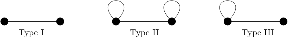
Figure 3. Connected graphs with 2 vertices.

For 2-dimensional representations, one can slightly strengthen the correspondence between representations and graphs. Before formulating this result, let us prove the following lemma which will later also be useful when discussing equivalence of representations.

Lemma 4.9.

Let $x_{1}\neq x_{2}$,

$$X=\begin{pmatrix}x_{1}&0\\ 0&x_{2}\end{pmatrix}\qquad\tilde{X}=\begin{pmatrix}\tilde{x}_{1}&0\\ 0&\tilde{x}_{2}\end{pmatrix}$$

and assume that there exists a unitary matrix $U$ such that $UXU^{\dagger}=\tilde{X}$. For an arbitrary hermitian matrix

$$Y=\begin{pmatrix}y_{1}&z\\ \bar{z}&y_{2}\end{pmatrix}$$

it follows that there exists $\varphi\in\mathbb{R}$ such that either

$$\tilde{X}=\begin{pmatrix}x_{1}&0\\ 0&x_{2}\end{pmatrix}\quad\text{and}\quad UYU^{\dagger}=\begin{pmatrix}y_{1}&e^{i\varphi}z\\ e^{-i\varphi}z&y_{2}\end{pmatrix}$$

or

$$\tilde{X}=\begin{pmatrix}x_{2}&0\\ 0&x_{1}\end{pmatrix}\quad\text{and}\quad UYU^{\dagger}=\begin{pmatrix}y_{2}&e^{-i\varphi}\bar{z}\\ e^{i\varphi}z&y_{1}\end{pmatrix}.$$

Proof.

Writing an arbitrary unitary $2\times 2$ matrix as

$$e^{\tilde{\varphi}/2}\begin{pmatrix}e^{i\varphi_{1}}\cos\theta&e^{i\varphi_{2}}\sin\theta\\ -e^{-i\varphi_{2}}\sin\theta&e^{-i\varphi_{1}}\cos\theta\end{pmatrix}$$

one finds that

$$UXU^{\dagger}=\begin{pmatrix}x_{1}\cos^{2}\theta+x_{2}\sin^{2}\theta&-\tfrac{1}{2}e^{i(\varphi_{1}+\varphi_{2})}(x_{1}-x_{2})\sin 2\theta\\ -\tfrac{1}{2}e^{i(\varphi_{1}+\varphi_{2})}(x_{1}-x_{2})\sin 2\theta&x_{1}\sin^{2}\theta+x_{2}\cos^{2}\theta\\ \end{pmatrix}.$$

For this matrix to be diagonal, a necessary condition is that $\sin 2\theta=0$ since $x_{1}\neq x_{2}$. Thus, $\theta=0,\pi/2,\pi,3\pi/2$ and it is easy to see that $UYU^{\dagger}$ has the required form for these values of $\theta$. ∎

Using the above result, one can prove that unitarily equivalent representations have isomorphic graphs.

Proposition 4.10.

If $\phi$ and $\phi^{\prime}$ are unitarily equivalent non-degenerate 2-dimensional representations of $\mathcal{C}_{\hbar}^{g}$, then the graph of $\phi$ is isomorphic to the graph of $\phi^{\prime}$.

Proof.

If $\phi$ is a non-degenerate representation with $\phi(X)=\operatorname{diag}(x_{1},x_{2})$ then one must necessarily have $x_{1}\neq x_{2}$ since, otherwise, $\phi(X)$ commutes with $\phi(Y)$ (giving $\phi(Z)=0$). Then one may apply Lemma 4.9 to conclude that $\phi(Y)$ and $\phi^{\prime}(Y)$ have exactly the same structure of non-zero matrix elements (up to a permutation of the rows and columns) implying that the corresponding graphs are isomorphic. ∎

In particular, it follows from the above result that representations with graphs of Type I and Type II are inequivalent. Now, let us turn to the task of finding concrete representations.

For a representation $\phi$ with

$$\phi(X)=\begin{pmatrix}x_{1}&0\\ 0&x_{2}\end{pmatrix}\qquad\phi(Y)=\begin{pmatrix}y_{1}&z\\ \bar{z}&y_{2}\end{pmatrix}$$

equations A_ij and B_ij become

(A₁₁) $$\big{(} 2(x_{1}-x_{2})-\hbar^{2}p(x_{1})\big{)}|z|^{2}-\hbar^{2}p^{\prime}(x_{1})y_{1}^{2}=\hbar^{2}p(x_{1})p^{\prime}(x_{1})$$

(A₂₂) $$\big{(}- 2(x_{1}-x_{2})-\hbar^{2}p(x_{2})\big{)}|z|^{2}-\hbar^{2}p^{\prime}(x_{2})y_{2}^{2}=\hbar^{2}p(x_{2})p^{\prime}(x_{2})$$

(A₁₂) $$z\big{(}q_{\hbar}(x_{1},x_{2})(y_{1}+y_{2})-2x_{1}y_{1}-2x_{2}y_{2}\big{)}=0$$

(B₁₁) $$y_{1}^{3}+(2y_{1}+y_{2})|z|^{2}+p(x_{1})y_{1}=0$$

(B₂₂) $$y_{2}^{3}+(2y_{2}+y_{1})|z|^{2}+p(x_{2})y_{2}=0$$

(B₁₂) $$y_{1}^{2}+y_{2}^{2}+y_{1}y_{2}+|z|^{2}=\tfrac{1}{2\hbar^{2}}r_{\hbar}(x_{1},x_{2}).$$

If $z\neq 0$ and $x_{1}=-x_{2}=x\neq 0$ the above equations are equivalent to

(4.4) $$\big{(}4x-\hbar^{2}p(x)\big{)}|z|^{2}-\hbar^{2}p^{\prime}(x)y^{2}=\hbar^{2}p(x)p^{\prime}(x)$$

(4.5) $$y\big{(}y^{2}+3|z|^{2}+p(x)\big{)}=0$$

(4.6) $$3y^{2}+|z|^{2}=\frac{2x^{2}}{\hbar^{2}}-p(x)$$

with $y_{1}=y_{2}=y$. Let us start by considering representations of Type I.

Proposition 4.11.

$\phi$ is a non-degenerate representation of $\mathcal{C}_{\hbar}^{g}$ such that

$$\phi(X)=\begin{pmatrix}\hat{x}&0\\ 0&-\hat{x}\end{pmatrix}\qquad\phi(Y)=\begin{pmatrix}0&z\\ \bar{z}&0\end{pmatrix}\qquad\phi(Z)=\frac{2i}{\hbar}\begin{pmatrix}0&-\hat{x}z\\ \hat{x}\bar{z}&0\end{pmatrix}$$

if and only if

$$z=\frac{1}{\hbar}e^{i\theta}\sqrt{2\hat{x}^{2}-\hbar^{2}p(\hat{x})}$$

for $\theta\in\mathbb{R}$ and $\hat{x}$ satisfying

(4.7) $$2p(\hat{x})+\hat{x}p^{\prime}(\hat{x})-\frac{4\hat{x}^{2}}{\hbar^{2}}=0$$

(4.8) $$2\hat{x}^{2}-\hbar^{2}p(\hat{x})>0.$$

Proof.

Let $X$ and $Y$ be matrices of a 2-dimensional non-degenerate representation of $\mathcal{C}_{\hbar}^{g}$ of the form above. Since $Z\neq 0$ we necessarily have $\hat{x},z\neq 0$. Equations (4.4)– (4.6) (with $y=0$) then become

$$\big{(}4x-\hbar^{2}p^{\prime}(x)\big{)}|z|^{2} =\hbar^{2}p(x)p^{\prime}(x)$$

$$|z|^{2} =\frac{2x^{2}}{\hbar^{2}}-p(x)$$

which are equivalent to

$$2p(x)+xp^{\prime}(x)-\frac{4x^{2}}{\hbar^{2}}=0$$

$$|z|^{2}=\frac{2x^{2}}{\hbar^{2}}-p(x).$$

The fact that $\phi$ is non-degenerate implies that $z\neq 0$ which necessarily gives $\frac{2x^{2}}{\hbar^{2}}-p(x)>0$, proving the first part of the statement.

Conversely, if $\hat{x}$ is a solution of (4.7) such that $\frac{2\hat{x}^{2}}{\hbar^{2}}-p(\hat{x})>0$ then one may construct a solution by setting

$$z=\frac{1}{\hbar}e^{i\theta}\sqrt{2\hat{x}^{2}-\hbar^{2}p(\hat{x})}\neq 0$$

for arbitrary $\theta\in\mathbb{R}$. Finally, to prove that $\phi$ is non-degenerate (i.e. $Z\neq 0)$, we need to show that $\hat{x}=0$ is never a solution to (4.7) and (4.8). If $\hat{x}=0$ is a solution to (4.7) then $p(\hat{x})=0$, which implies that $\frac{2\hat{x}^{2}}{\hbar^{2}}-p(\hat{x})=0$, which does not fulfill (4.8). Hence, any solution to (4.7) and (4.8) is non-zero. ∎

The next result ensures that one may find a Type I representation of $\mathcal{C}_{\hbar}^{g}$ for any value of the deformation parameter $\hbar>0$.

Proposition 4.12.

For $\hbar>0$ and $g\geq 2$, there exists $\hat{x}>g-1$ such that

$$2p(\hat{x})+\hat{x}p^{\prime}(\hat{x})-\frac{4\hat{x}^{2}}{\hbar^{2}}=0\quad\text{and}\quad\frac{2\hat{x}^{2}}{\hbar^{2}}-p(\hat{x})>0.$$

Proof.

First we note that if $2p(\hat{x})+\hat{x}p^{\prime}(\hat{x})-4\hat{x}^{2}/\hbar^{2}=0$ and $\hat{x}p^{\prime}(\hat{x})>0$ then

$$\frac{2\hat{x}^{2}}{\hbar^{2}}-p(\hat{x})=\frac{2\hat{x}^{2}}{\hbar^{2}}+\frac{1}{2}\hat{x}p^{\prime}(\hat{x})-\frac{2\hat{x}^{2}}{\hbar^{2}}=\frac{1}{2}\hat{x}p^{\prime}(\hat{x})>0.$$

Writing $f_{\hbar}(x)=2p(x)+xp^{\prime}(x)-4x^{2}/\hbar^{2}$ one finds that

$$f_{\hbar}(g-1)=-2\sqrt{c}+(g-1)p^{\prime}(g-1)-\frac{4(g-1)^{2}}{\hbar^{2}}<0$$

since $p^{\prime}(g-1)<0$ (cf. (2.1)). For $g\geq 2$, $f_{\hbar}(x)$ is a polynomial of degree $2g$ with a positive coefficient of $x^{2g}$, which implies that $f_{\hbar}(x)$ is positive for large $x$. In particular, there exists $\hat{x}>g-1$ such that $f_{\hbar}(\hat{x})=0$. If $\hat{x}\geq g$ then $\hat{x}p^{\prime}(\hat{x})>0$ since $xp^{\prime}(x)>0$ for all $x\geq g$. If $\hat{x}\in(g-1,g)$ and $f_{\hbar}(\hat{x})=0$ then $\hat{x}p^{\prime}(\hat{x})>0$ due to the fact that $p(x)<0$ for all $x\in(g-1,g)$ and

$$\hat{x}p^{\prime}(\hat{x})=\frac{4\hat{x}^{2}}{\hbar^{2}}-2p(\hat{x}).$$

From the argument in the beginning of the proof, it follows that

$$2\hat{x}^{2}/\hbar^{2}-p(\hat{x})>0.\qed$$

In the case when $g=1$, one obtains

$$2p(x)+xp^{\prime}(x)-\frac{4x^{2}}{\hbar^{2}}=4x^{2}\Big{(}\alpha-\frac{1}{\hbar^{2}}\Big{)}-2(\alpha+\sqrt{c})$$

which does not have any real solutions for small enough $\hbar$. However, this case has been treated thoroughly in [ABH⁺09a, ABH⁺09b].

In any case, we have shown the existence of representations for arbitrary $g\geq 2$ and values of the deformation parameter $\hbar$. Let us state this result as follows.

Corollary 4.13.

For $g\geq 2$, $\hbar>0$, $c>0$ and $\alpha\in(0,2\sqrt{c}/M)$, there exists a 2-dimensional non-degenerate representation of $\mathcal{C}_{\hbar}^{g}(\alpha,c)$.

Next, we consider representations of Type II.

Proposition 4.14.

$\phi$ is a non-degenerate representation of $\mathcal{C}_{\hbar}^{g}$ such that

$$\phi(X)=\begin{pmatrix}\hat{x}&0\\ 0&-\hat{x}\end{pmatrix}\qquad\phi(Y)=\begin{pmatrix}y_{1}&z\\ \bar{z}&y_{2}\end{pmatrix}\qquad\phi(Z)=\frac{2i}{\hbar}\begin{pmatrix}0&-\hat{x}z\\ \hat{x}\bar{z}&0\end{pmatrix}$$

with $y_{1}\neq 0$, if and only if

$$y_{1}=y_{2}=\pm\frac{1}{2\hbar} \sqrt{3\hat{x}^{2}-\hbar^{2}p(\hat{x})}$$

$$z=\frac{1}{2\hbar}e^{i\theta} \sqrt{-\hat{x}^{2}-\hbar^{2}p(\hat{x})}$$

for $\theta\in\mathbb{R}$ and $\hat{x}\neq 0$ satisfying

(4.9) $$2p(\hat{x})-\hat{x}p^{\prime}(\hat{x})<0$$

(4.10) $$2\hat{x}+\hbar^{2}p^{\prime}(\hat{x})=0.$$

Proof.

Assume that $X$ and $Y$ are matrices of a non-degenerate 2-dimensional representation of the form above with $y_{1}\neq 0$. Since $Z\neq 0$, we necessarily have that $\hat{x},z\neq 0$. As already noted, when $x_{1}=-x_{2}$ and $z\neq 0$, equation A₁₂ implies that $y_{1}=y_{2}=y$. Since $y=y_{1}\neq 0$, equations (4.4)–(4.6) become

$$\big{(}4x-\hbar^{2}p(x)\big{)}|z|^{2}-\hbar^{2}p^{\prime}(x)y^{2}=\hbar^{2}p(x)p^{\prime}(x)$$

$$y^{2}+3|z|^{2}+p(x)=0$$

$$3y^{2}+|z|^{2}=\frac{2x^{2}}{\hbar^{2}}-p(x)$$

which are equivalent to

(4.11) $$\big{(}2x+\hbar^{2}p^{\prime}(x)\big{)}\big{(}x^{2}+\hbar^{2}p(x)\big{)}=0$$

(4.12) $$y^{2}=\frac{1}{4\hbar^{2}}\big{(}3x^{2}-\hbar^{2}p(x)\big{)}$$

(4.13) $$|z|^{2}=-\frac{1}{4\hbar^{2}}\big{(}x^{2}+\hbar^{2}p(x)\big{)}.$$

From (4.11) it follows that either $2x+\hbar^{2}p^{\prime}(x)=0$ or $x^{2}+\hbar^{2}p(x)=0$. However, if $x^{2}+\hbar^{2}p(x)=0$ then $z=0$, which contradicts the assumption that $\phi$ is non-degenerate. Hence, it must hold that $2\hat{x}+\hbar^{2}p^{\prime}(\hat{x})=0$. Moreover, from (4.13) it follows that $\hat{x}^{2}+\hbar^{2}p(\hat{x})<0$ which, by inserting $\hat{x}^{2}=-\tfrac{1}{2}\hbar^{2}\hat{x}p^{\prime}(\hat{x})$ gives $2p(\hat{x})-\hat{x}p^{\prime}(\hat{x})<0$. Conversely, assume that (4.9) and (4.10) holds for some $\hat{x}\in\mathbb{R}$, giving

$$\hat{x}p^{\prime}(\hat{x})=-\frac{2\hat{x}^{2}}{\hbar^{2}}\quad\text{and}\quad\hat{x}^{2}+\hbar^{2}p(\hat{x})<0,$$

implying that (4.13) is satisfied by defining

$$z=\frac{1}{2\hbar}e^{i\theta} \sqrt{|\hat{x}^{2}+\hbar^{2}p(\hat{x})|}\neq 0$$

for arbitrary $\theta\in\mathbb{R}$. Moreover, since $\hat{x}^{2}+\hbar^{2}p(\hat{x})<0$ it follows that

$$3\hat{x}^{2}-\hbar^{2}p(\hat{x})>3\hat{x}^{2}+\hat{x}^{2}=4\hat{x}^{2}>0,$$

implying that

$$y=\pm\frac{1}{2\hbar} \sqrt{3\hat{x}^{2}-\hbar^{2}p(\hat{x})}\neq 0$$

solves (4.12). Finally, equation (4.11) is satisfied since $2\hat{x}+\hbar^{2}p^{\prime}(\hat{x})=0$. The representation defined in this way will be non-degenerate since $\hat{x}\neq 0$ (by assumption) and $z\neq 0$ due to $\hat{x}^{2}+\hbar^{2}p(\hat{x})<0$. ∎

Thus, to construct a representation of Type II as in Proposition 4.14 one needs to find $\hat{x}$ such that

$$2p(\hat{x})-\hat{x}p^{\prime}(\hat{x})<0$$

$$2\hat{x}+\hbar^{2}p^{\prime}(\hat{x})=0.$$

It is useful to think of the second equation as determining $\hbar$. That is, for any $\hat{x}\in\mathbb{R}$ such that $p^{\prime}(\hat{x})<0$, we can consider Type II representations of $\mathcal{C}_{\hbar}^{g}$ with

$$\hbar=\sqrt{-\frac{2\hat{x}}{p^{\prime}(\hat{x})}}$$

satisfying $2\hat{x}+\hbar^{2}p^{\prime}(\hat{x})=0$. The next result guarantees one may find such an $\hat{x}$ also satisfying $2p(\hat{x})-\hat{x}p^{\prime}(\hat{x})<0$.

Proposition 4.15.

If $\alpha/\sqrt{c}<2/(2g-1)!$ then

$$p^{\prime}(g-1)<0\quad\text{and}\quad 2p(g-1)-(g-1)p^{\prime}(g-1)<0.$$

Proof.

One notes immediately that $p^{\prime}(g-1)<0$ from (2.1). Moreover, one obtains

$$2p(g-1)-(g-1)p^{\prime}(g-1) =-2\sqrt{c}+\alpha(2g-1)!$$

$$=\sqrt{c}(2g-1)!\Big{(}\frac{\alpha}{\sqrt{c}}-\frac{2}{(2g-1)!}\Big{)}<0$$

by assumption. ∎

Hence, for $\alpha/\sqrt{c}<2/(2g-1)!$ one may construct a Type II representation of $\mathcal{C}_{\hbar}^{g}$ as in Proposition 4.14 with

$$\hbar=\sqrt{-\frac{2(g-1)}{p^{\prime}(g-1)}}=\sqrt{\frac{2(g-1)^{2}}{\alpha(2g-1)!}}$$

and $\hat{x}=g-1$, giving

$$y=\pm\frac{1}{2}\sqrt{\sqrt{c}+\tfrac{3}{2}\alpha(2g-1)!}$$

$$z=\frac{1}{2}e^{i\theta}\sqrt{\sqrt{c}-\tfrac{1}{2}\alpha(2g-1)!}.$$

The above considerations illustrate a property which is generic in the context of matrix regularizations. Namely, the deformation parameter $\hbar$ is related to the dimension of the representation giving restrictions on for which $\hbar$ an $N$-dimensional representation may exist.

It is clear from Proposition 4.10 that representations of Type I and II are not equivalent. However, we would like to investigate to what extent there are inequivalent representations of the same type.

Proposition 4.16.

Let $\phi$ and $\phi^{\prime}$ be representations as in Proposition 4.11 with

$$\phi(X)=\begin{pmatrix}\hat{x}&0\\ 0&-\hat{x}\end{pmatrix}\quad\text{and}\quad\phi^{\prime}(X)=\begin{pmatrix}\hat{x}^{\prime}&0\\ 0&-\hat{x}^{\prime}\end{pmatrix}.$$

Then $\phi$ is unitarily equivalent to $\phi^{\prime}$ if and only if $\hat{x}=\pm\hat{x}^{\prime}$.

Proof.

First, assume that $\phi$ and $\phi^{\prime}$ are unitarily equivalent representations as in Proposition 4.11. Since the diagonal elements of $\phi(X)$ are distinct (due to the assumption that $\phi$ is non-degenerate) one may apply Lemma 4.9 to conclude that either $\hat{x}^{\prime}=\hat{x}$ or $\hat{x}^{\prime}=-\hat{x}$.

Next, assume that $\phi$ and $\phi^{\prime}$ are representations as in Proposition 4.11 such that $\hat{x}^{\prime}=\hat{x}$ and

$$\phi(Y)=\frac{1}{\hbar}\sqrt{2\hat{x}^{2}-\hbar^{2}p(\hat{x})}\begin{pmatrix}0&e^{i\theta}\\ e^{-i\theta}&0\end{pmatrix}$$

$$\phi^{\prime}(Y)=\frac{1}{\hbar}\sqrt{2\hat{x}^{2}-\hbar^{2}p(\hat{x})}\begin{pmatrix}0&e^{i\theta^{\prime}}\\ e^{-i\theta^{\prime}}&0\end{pmatrix}.$$

It is easy to see that these matrices are indeed unitarily equivalent with $\phi^{\prime}(Y)=U\phi(Y)U^{\dagger}$ for $U=\operatorname{diag}(e^{i\theta^{\prime}},e^{i\theta})$. The argument for $\hat{x}^{\prime}=-\hat{x}$ is analogous and uses the fact that $p(-\hat{x})=p(\hat{x})$. ∎

The result for representations of Type II is similar.

Proposition 4.17.

Let $\phi$ and $\phi^{\prime}$ be representations as in Proposition 4.14 with

$$\phi(X)=\begin{pmatrix}\hat{x}&0\\ 0&-\hat{x}\end{pmatrix} \phi(Y)=\begin{pmatrix}y&z\\ \bar{z}&y\end{pmatrix}$$

$$\phi^{\prime}(X)=\begin{pmatrix}\hat{x}^{\prime}&0\\ 0&-\hat{x}^{\prime}\end{pmatrix} \phi^{\prime}(Y)=\begin{pmatrix}y^{\prime}&z^{\prime}\\ \bar{z}^{\prime}&y^{\prime}\end{pmatrix}.$$

Then $\phi$ is unitarily equivalent to $\phi^{\prime}$ if and only if $\hat{x}=\pm\hat{x}^{\prime}$ and $y=y^{\prime}$.

Proof.

The proof is in complete analogy with the proof of Proposition 4.16 and will not be repeated in detail. The only slight difference is that there is a choice of sign in $y$ which can not be compensated for by a unitary transformation. ∎

4.4. A 3-dimensional representation

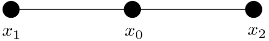
Figure 4. An admissible graph on three vertices.

Let us give an example of a 3-dimensional representation with a graph as in Figure 4. Equations A_ij and B_ij become

(A₀₀) $$\big{(}2(x_{0}-x_{1}) -\hbar^{2}p^{\prime}(x_{0})\big{)}|z_{1}|^{2}+\big{(}2(x_{0}-x_{2})-\hbar^{2}p^{\prime}(x_{0})\big{)}|z_{2}|^{2}=\hbar^{2}p(x_{0})p^{\prime}(x_{0})$$

(A₁₁) $$\big{(}2(x_{1}-x_{0})-\hbar^{2}p^{\prime}(x_{1})\big{)}|z_{1}|^{2}=\hbar^{2}p(x_{1})p^{\prime}(x_{1})$$

(A₂₂) $$\big{(}2(x_{2}-x_{0})-\hbar^{2}p^{\prime}(x_{2})\big{)}|z_{2}|^{2}=\hbar^{2}p(x_{2})p^{\prime}(x_{2})$$

(A₁₂) $$x_{0}=\frac{1}{2}q_{\hbar}(x_{1},x_{2})$$

(B₀₁) $$2\hbar^{2}\big{(}|z_{1}|^{2}+|z_{2}|^{2}\big{)}=r_{\hbar}(x_{0},x_{1})$$

(B₀₂) $$2\hbar^{2}\big{(}|z_{1}|^{2}+|z_{2}|^{2}\big{)}=r_{\hbar}(x_{0},x_{2}).$$

where $z_{1}=y_{01}$ and $z_{2}=y_{02}$. For $x_{0}=0$, $x_{1}=-x_{2}=x$ one uses $q_{\hbar}(x,-x)=0$ and $p^{\prime}(0)=0$ to show that the equations are equivalent to

(A₀₀) $$r=|z_{1}|=|z_{2}|$$

(A₁₁) $$\big{(}2x-\hbar^{2}p^{\prime}(x)\big{)}r^{2}=\hbar^{2}p(x)p^{\prime}(x)$$

(B₀₁) $$4\hbar^{2}r^{2}=x^{2}-\hbar^{2}\big{(}p(0)+p(x)\big{)}.$$

Proposition 4.18.

If $\hat{x}^{2}-\hbar^{2}\big{(}p(0)+p(\hat{x})\big{)}>0$, $\hat{x}\neq 0$ and

$$\bigg{(}\frac{2\hat{x}}{\hbar^{2}}-p^{\prime}(\hat{x})\bigg{)}\bigg{(}\frac{\hat{x}^{2}}{\hbar^{2}}-p(0)-p(\hat{x})\bigg{)}=4p(\hat{x})p^{\prime}(\hat{x})$$

then

$$\phi(X)=\begin{pmatrix}0&0&0\\ 0&\hat{x}&0\\ 0&0&-\hat{x}\end{pmatrix}\quad\phi(Y)=\begin{pmatrix}0&z_{1}&z_{2}\\ \bar{z}_{1}&0&0\\ \bar{z}_{2}&0&0\end{pmatrix}\quad\phi(Z)=\frac{i\hat{x}}{\hbar}\begin{pmatrix}0&z_{1}&-z_{2}\\ -\bar{z}_{1}&0&0\\ \bar{z}_{2}&0&0\end{pmatrix}$$

with

$$z_{1}=\frac{1}{2\hbar}e^{i\theta_{1}}\sqrt{\hat{x}^{2}-\hbar^{2}\big{(}p(\hat{x})+p(0)\big{)}}$$

$$z_{2}=\frac{1}{2\hbar}e^{i\theta_{2}}\sqrt{\hat{x}^{2}-\hbar^{2}\big{(}p(\hat{x})+p(0)\big{)}},$$

for $\theta_{1},\theta_{2}\in\mathbb{R}$, define a non-degenerate representation of $\mathcal{C}_{\hbar}^{g}$.

There are several ways of satisfying the requirements of Proposition 4.18, and let us give a particular construction in the next result. To this end, let us introduce the following notation

$$f_{\hbar}(x)=\bigg{(}\frac{2x}{\hbar^{2}}-p^{\prime}(x)\bigg{)}\bigg{(}\frac{x^{2}}{\hbar^{2}}-p(0)-p(x)\bigg{)}-4p(x)p^{\prime}(x)$$

$$r_{\hbar}(x)=\frac{x^{2}}{4\hbar^{2}}-\frac{1}{4}\big{(}p(0)+p(x)\big{)}.$$

Proposition 4.19.

There exists $\hbar>0$ such that

$$f_{\hbar}(g-1)=0\quad\text{and}\quad r_{\hbar}(g-1)>0.$$

Proof.

Expanding $f_{\hbar}$ gives

$$f_{\hbar}(x)=\frac{2x^{3}}{\hbar^{4}}-\frac{1}{\hbar^{2}}\big{(}p(0)+p(x)+p^{\prime}(x)\big{)}+p^{\prime}(x)\big{(}p(0)-3p(x)\big{)}$$

If $x>0$ then $f_{\hbar}(x)>0$ for small enough $\hbar$, and if $p^{\prime}(x)\big{(}p(0)-3p(x)\big{)}<0$ then $f_{\hbar}(x)<0$ for large enough $\hbar$. Thus, for such an $x$, there exists $\hbar>0$ such that $f_{\hbar}(x)=0$. Let us now show that $x=g-1$ fulfills

$$p^{\prime}(g-1)\big{(}p(0)-3p(g-1)\big{)}=p^{\prime}(g-1)\big{(}p(0)+3\sqrt{c}\big{)}<0.$$

Since $p^{\prime}(g-1)<0$ the above is equivalent to $p(0)+3\sqrt{c}>0$ which is true by Lemma 2.2. Next, let us show that $r_{\hbar}(g-1)>0$ for all $\hbar>0$:

$$r_{\hbar}(g-1)=\frac{(g-1)^{2}}{4\hbar^{2}}-\frac{1}{4}\big{(}p(0)-\sqrt{c}\big{)}>0$$

since Lemma 2.2 gives $p(0)-\sqrt{c}<0$. ∎

Thus, for $\hat{x}=g-1$ and $\hbar$ as in Proposition 4.19 we find that

$$z_{1}=\frac{1}{2\hbar}e^{i\theta_{1}}\sqrt{(g-1)^{2}-\hbar^{2}\big{(}(-1)^{g}\alpha(g!)^{2}-2\sqrt{c}\big{)}}$$

$$z_{2}=\frac{1}{2\hbar}e^{i\theta_{2}}\sqrt{(g-1)^{2}-\hbar^{2}\big{(}(-1)^{g}\alpha(g!)^{2}-2\sqrt{c}\big{)}}.$$

Furthermore, it is clear that the phases $\theta_{1}$ and $\theta_{2}$ are inessential as one may always find an equivalent representation with $\theta_{1}=\theta_{2}=0$ by conjugating with a diagonal unitary matrix. Finally, let us show that these representations are irreducible.

Proposition 4.20.

If $\phi$ is a representation of $\mathcal{C}_{\hbar}^{g}$ as in Proposition 4.18 then $\phi$ is irreducible.

Proof.

If $\phi$ is reducible, then $\phi$ is completely reducible to a sum of lower dimensional representations, which implies that $\phi$ is equivalent to a representation with at least two disconnected components in the corresponding graph. Since $\hat{x}\neq 0$ the three eigenvalues of $X$ are distinct, which implies that unitary matrices $U$, such that $UXU^{\dagger}$ is again diagonal, are composed of permutations and diagonal unitary matrices. Hence, the graph of $Y$ is isomorphic to the graph of $UYU^{\dagger}$, which implies that $UYU^{\dagger}$ is connected. We conclude that $\phi$ is irreducible. ∎

5. Concluding remarks

Finding matrix regularizations for surfaces of higher genus seems to be a notoriously difficult problem. The simple structure of representations in the case of genus 0 and 1, does not lend itself to any easy generalizations. In this paper, we have followed the idea of finding representations of a one-parameter family of deformations of a commutative algebra (corresponding to smooth functions on the surface), in order to generate a matrix regularization. These algebras have a concrete definition in terms of generators and relations in direct correspondence with the definition of surfaces as level sets in $\mathbb{R}^{3}$. Explicit low-dimensional representations have been constructed, but ideally one would like a complete sequence of matrix algebras (of increasing dimension) for a sequence of the deformation parameter $\hbar$ tending to zero. Although we have not reached our final goal, we believe that our investigation has considerably increased the understanding of representations, as well as the analytic structure of the defining polynomials, paving the way for future work.

References

• [ABH+09a] J. Arnlind, M. Bordemann, L. Hofer, J. Hoppe, and H. Shimada. Fuzzy Riemann surfaces. JHEP, 06:047, 2009.
• [ABH+09b] J. Arnlind, M. Bordemann, L. Hofer, J. Hoppe, and H. Shimada. Noncommutative Riemann surfaces by embeddings in $\mathbb{R}^{3}$. Comm. Math. Phys., 288(2):403–429, 2009.
• [AH10] J. Arnlind and J. Hoppe. Discrete minimal surface algebras. SIGMA, 6:042, 2010.
• [AHH12] J. Arnlind, J. Hoppe, and G. Huisken. Multi-linear formulation of differential geometry and matrix regularizations. J. Differential Geom., 91(1):1–39, 2012.
• [Arn08a] J. Arnlind. Graph Techniques for Matrix Equations and Eigenvalue Dynamics. PhD thesis, Royal Institute of Technology, 2008.
• [Arn08b] J. Arnlind. Representation theory of $C$-algebras for a higher-order class of spheres and tori. J. Math. Phys., 49(5):053502, 13, 2008.
• [BHSS91] M. Bordemann, J. Hoppe, P. Schaller, and M. Schlichenmaier. ${\rm gl}(\infty)$ and geometric quantization. Comm. Math. Phys., 138(2):209–244, 1991.
• [BMS94] M. Bordemann, E. Meinrenken, and M. Schlichenmaier. Toeplitz quantization of Kähler manifolds and ${\rm gl}(N)$, $N\to\infty$ limits. Comm. Math. Phys., 165(2):281–296, 1994.
• [dWHN88] B. de Wit, J. Hoppe, and H. Nicolai. On the quantum mechanics of supermembranes. Nuclear Phys. B, 305(4, FS23):545–581, 1988.
• [FFZ89] D. B. Fairlie, P. Fletcher, and C. K. Zachos. Trigonometric structure constants for new infinite-dimensional algebras. Phys. Lett. B, 218(2):203–206, 1989.
• [Hof07] L. Hofer. Aspects algébriques et quantification des surfaces minimales. PhD thesis, Université de Haute-Alsace, 2007.
• [Hop82] J. Hoppe. Quantum Theory of a Massless Relativistic Surface and a Two-dimensional Bound State Problem. PhD thesis, Massachusetts Institute of Technology, 1982.
• [Hop88] J. Hoppe. ${\rm Diff}_{A}T^{2},$ and the curvature of some infinite-dimensional manifolds. Phys. Lett. B, 215(4):706–710, 1988.
• [Hop89] J. Hoppe. Diffeomorphism groups, quantization, and ${\rm SU}(\infty)$. Internat. J. Modern Phys. A, 4(19):5235–5248, 1989.
• [IKKT97] N. Ishibashi, H. Kawai, Y. Kitazawa, and A. Tsuchiya. A Large N reduced model as superstring. Nucl.Phys., B498:467–491, 1997.
• [KL92a] S. Klimek and A. Lesniewski. Quantum Riemann surfaces. I. The unit disc. Comm. Math. Phys., 146(1):103–122, 1992.
• [KL92b] S. Klimek and A. Lesniewski. Quantum Riemann surfaces. II. The discrete series. Lett. Math. Phys., 24(2):125–139, 1992.
• [KL94] S. Klimek and A. Lesniewski. Quantum Riemann surfaces. III. The exceptional cases. Lett. Math. Phys., 32(1):45–61, 1994.
• [Mad92] J. Madore. The fuzzy sphere. Classical Quantum Gravity, 9(1):69–87, 1992.
• [NN99] T. Natsume and R. Nest. Topological approach to quantum surfaces. Comm. Math. Phys., 202(1):65–87, 1999.
• [Shi04] H. Shimada. Membrane topology and matrix regularization. Nuclear Phys. B, 685:297–320, 2004.
• [Ste10] H. Steinacker. Emergent geometry and gravity from matrix models: an introduction. Classical Quantum Gravity, 27(13):133001, 46, 2010.
• [Syk16] A. Sykora. The fuzzy space construction kit. arXiv:1610.01504, 2016.