Swift/XRT- NuSTAR spectra of type 1 AGN: confirming INTEGRAL results on the high energy cut-off

Abstract

We present the 0.5 – 78 keV spectral analysis of 18 broad line AGN belonging to the INTEGRAL complete sample. Using simultaneous Swift-XRT and NuSTAR observations and employing a simple phenomenological model to fit the data, we measure with a good constraint the high energy cut-off in 13 sources, while we place lower limits on 5 objects. We found a mean high-energy cut-off of 111 keV ($\sigma$ = 45 keV) for the whole sample, in perfect agreement with what found in our previous work using non simultaneous observations and with what recently published using NuSTAR data. This work suggests that simultaneity of the observations in the soft and hard X-ray band is important but not always essential, especially if flux and spectral variability are properly accounted for. A lesser agreement is found when we compare our cut-off measurements with the ones obtained by Ricci et al. (2017) using Swift-BAT high energy data, finding that their values are systematically higher than ours. We have investigated whether a linear correlation exists between photon index and the cut-off and found a weak one, probably to be ascribed to the non perfect modelling of the soft part of the spectra, due to the poor statistical quality of the 2-10 keV X-ray data. No correlation is also found between the Eddington ratio and the cut-off, suggesting that only using high statistical quality broad-band spectra is it possible to verify the theoretical predictions and study the physical characteristics of the hot corona and its geometry.

1 Introduction

In recent years, high energy observations of Active Galactic Nuclei (AGN) have provided new insights on the physics and mechanisms at play in some of the most energetic phenomena in the Universe. In particular, the slope of the continuum emission and its high energy cut-off are essential for spectral modelling of AGN, since these parameters directly probe the physical characteristics of the Comptonizing region around the central nucleus. Indeed the X-ray continuum of AGN can be ascribed to the inverse Compton scattering of soft photons arising from the accretion disc by energetic electrons thermally distributed above the disc, the so-called X-ray corona. Clearly to have an overview of the physics and structure of the corona we need to study the broad-band spectra of a large sample of AGN in order to account for all spectral components, remove the degeneracy between parameters and therefore being able to obtain a precise estimate of the photon index and high energy cut-off for a large number of objects.

Many independent observations in the X-rays suggest that the corona should be compact and located very close to the black hole, but its characteristics are still largely unknown as only recently information on the electron temperature (cut-off energy) and the optical depth (photon index) of the hot plasma in the corona has become available. Furthermore, very little is known about the heating and thermalization mechanisms operating in the corona, i.e. what controls the plasma temperature and how any stable equilibrium is reached (Fabian et al. 2015, Fabian et al. 2017). Recently, Malizia et al. (2014) and Ricci et al. (2017) have analysed large samples of type 1 AGN and, through broad-band spectra covering a large energy range (typically from few keV up to hundreds of keV), found that the cut-off energy distribution peaks at around 100 keV, a result which is consistent with synthesis models of the Cosmic X-ray Background which locate the cut-off below 200 keV in order not to exceed it (Gilli et al., 2007). These first estimates of the temperature of the corona and its compactness parameter indicate that this region is hot and radiatively compact, that pair production and annihilation are essential mechanisms operating in it and that thermal and non thermal particles are present (Fabian et al. 2015; Fabian et al. 2017).

Table 1 - Observation Log

Source	XRT Obs. Date	XRT exposure	NuSTAR Obs. Date	NuSTAR exposure
		(ksec)		(ksec)
QSO B0241+62	30 July 2016	6.5	31 July 2016	23.3
MCG+08-11-011	18 Aug. 2016	15.9	18 Aug. 2016	97.9
Mrk 6	08-10 Nov. 2015	15.8	9 Nov. 2015	43.8
FRL 1146	28 July 2014	6.1	27 July 2014	21.3
IGR J12415-5750	27 Apr. 2016	5.7	27 Apr. 2016	16.4
4U 1344-60	17 Sep. 2016	1.8	17 Sep. 2016	99.5
IC 4329A	14 Aug. 2012	2.2	12 Aug. 2012	16.2
IGR J16119-6036	27 Apr. 2018	6.8	28 Apr. 2018	22
IGR J16482-3036	3 Apr. 2017	7.1	3 Apr. 2017	18.9
GRS 1734-292	16 Sep. 2014	6.2	16 Sep. 2014	20.2
2E 1739.1-1210	17 Oct. 2017	6.9	17 Oct. 2017	21.4
IGR J18027-1455	2 May 2016	6.6	2 May 2016	19.9
3C 390.3	25 May 2013	2.1	24 May 2013	47.6
2E 1853.7+1534	13 Oct. 2017	6.4	13 Oct. 2017	21.3
NGC 6814	05 July 2016	7.6	04 July 2016	148.4
4C 74.26	21 Sep. 2014	2.2	21 Sep. 2014	19.0
	24 Sep. 2014	2.0	22 Sep. 2014	56.5
	31 Oct. 2014	1.8	30 Oct. 2014	90.9
	22 Dec. 2014	2.1	22 Dec. 2014	42.7
S5 2116+81	5 Aug. 2017	6.7	5 Aug. 2017	18.5
IGR J21247+5058	13 Dec. 2014	6.8	13 Dec. 2014	24.3

However, these initial works made use of non-simultaneous low versus high energy data, and despite the introduction of cross-calibration constants to properly take into account flux variability (and possible mismatches in the instruments calibration), some degree of uncertainty remains due to the fact that the broad-band spectra are a combination of snapshot observations in the soft X-rays (typically from XMM-Newton or from Swift-XRT) with time-averaged (on timescales of years) spectra at high energies (INTEGRAL-IBIS, Swift-BAT). Despite the non-simultaneity of the data, cross-calibration constants are typically found to be close to 1 (Molina et al. 2009; Malizia et al. 2014), hinting at the fact that long-term flux variability can be easily accounted for in modelling of spectra taken in different epochs. Spectral variability, however, cannot be excluded a priori, making this the only uncertainty on an otherwise statistically robust result. If one wants to remove this ambiguity, it is fundamental to have simultaneous observations in both the soft and hard X-ray bands. This is now achievable thanks to the advent of NuSTAR, which is complementary, at least for bright sources, to INTEGRAL/IBIS and Swift/BAT in combination with soft X-ray data. In fact, several studies have been published recently which confirm, through simultaneous, high quality broad-band NuSTAR/XMM-Newton observations, what was previously found using non-contemporaneous data. However, it is not easy to obtain this type of high quality broad-band spectra and it is for this reason that sometime non-contemporaneous NuSTAR/soft X-ray observations are used preferring quality over simultaneity (e.g. Tortosa et al. 2017).

The main objective of this paper is to verify what was previously established from the broad-band spectral analysis of non-simultaneous XMM-Newton, INTEGRAL/IBIS and Swift/BAT spectra, in order to establish whether variability has still some effect on the spectral fits. If we find that for a significant sample of AGN the cut-off values are similar, either using simultaneous broad-band observations or not, than we can safely assume that spectral variability is not a big issue. Also, we aim at putting firmer constraints on the value of the high energy cut-off. Besides, we also attempt to establish whether choosing to use relatively simple, phenomenological models (like the pexrav model, which is more suitable for low statistics broad-band spectra) over more complex and more physical ones can nonetheless provide accurate measurements of the high energy cut-off.

Table 2- pexrav model fit results
Name	N${}_{\rm\bf H}^{\rm\bf FC}$	N${}_{\rm\bf H}^{\rm\bf PC}$ (cf)	$\Gamma$	Ec	R	EW	CFPMA	CFPMB	$\chi^{2}_{\nu}$
	(1022 cm-2)	(1022 cm-2)		(keV)		(eV)
QSO B0241+62	0.32${}^{+0.23}_{-0.19}$	–	1.82${}^{+0.07}_{-0.06}$	$>$ 198	0.72${}^{+0.35}_{-0.28}$	85${}^{+30}_{-28}$	1.53${}^{+0.21}_{-0.15}$	1.56${}^{+0.22}_{-0.18}$	1.00
MCG+08-11-011⋆	–	–	1.80${}^{+0.01}_{-0.01}$	163${}^{+53}_{-32}$	0.36${}^{+0.09}_{-0.08}$	128${}^{+17}_{-17}$	1.19${}^{+0.03}_{-0.03}$	1.24${}^{+0.03}_{-0.03}$	1.01
Mrk 6	–	9.92${}^{+1.73}_{-7.01}$ (0.95${}^{+0.02}_{-0.02}$)	1.73 (fixed)	120${}^{+51}_{-28}$	1.33${}^{+0.41}_{-0.37}$	82${}^{+31}_{-30}$	1.44${}^{+0.13}_{-0.11}$	1.47${}^{+0.13}_{-0.11}$	0.93
		22.4${}^{+8.60}_{-6.70}$ (0.51${}^{+0.05}_{-0.05}$)
FRL 1146	0.70${}^{+0.08}_{-0.13}$	–	2.07${}^{+0.09}_{-0.07}$	$>$182	1.03${}^{+0.42}_{-0.32}$	144${}^{+44}_{-44}$	1.09${}^{+0.09}_{-0.08}$	1.14${}^{+0.09}_{-0.09}$	1.07
IGR J12415-5750	–	–	1.63${}^{+0.05}_{-0.05}$	123${}^{+54}_{-47}$	$<$0.23	65${}^{+20}_{-30}$	1.41${}^{+0.09}_{-0.07}$	1.45${}^{+0.09}_{-0.08}$	0.97
4U 1344-60⋆	–	1.68${}^{+0.59}_{-0.22}$ ($>$0.83)	1.91${}^{+0.05}_{-0.03}$	141${}^{+46}_{-26}$	1.16${}^{+0.19}_{-0.16}$	109${}^{+21}_{-19}$	1.13${}^{+0.10}_{-0.08}$	1.19${}^{+0.10}_{-0.09}$	1.08
IC 4329A⋆	0.54${}^{+0.06}_{-0.05}$	–	1.73${}^{+0.01}_{-0.01}$	153${}^{+20}_{-16}$	0.43${}^{+0.05}_{-0.05}$	83${}^{+9}_{-8}$	1.17${}^{+0.06}_{-0.05}$	1.22${}^{+0.06}_{-0.06}$	1.01
IGR J16119-6036	–	–	1.57${}^{+0.08}_{-0.04}$	69${}^{+102}_{-26}$	0.40${}^{+0.56}_{-0.34}$	147${}^{+52}_{-49}$	0.95${}^{+0.07}_{-0.06}$	0.96${}^{+0.07}_{-0.06}$	1.09
IGR J16482-3036	–	–	1.63${}^{+0.11}_{-0.18}$	$>$38	0 (fixed)	163${}^{+173}_{-136}$	1.53${}^{+0.34}_{-0.28}$	1.59 ${}^{+0.34}_{-0.29}$	0.87
GRS 1734-292	1.08${}^{+0.15}_{-0.18}$	–	1.64${}^{+0.06}_{-0.06}$	53${}^{+13}_{-9}$	0.45${}^{+0.28}_{-0.24}$	34${}^{+23}_{-24}$	0.98${}^{+0.05}_{-0.05}$	1.07${}^{+0.05}_{-0.05}$	1.07
2E 1739.1-1210	0.16${}^{+0.06}_{-0.05}$	–	1.91${}^{+0.09}_{-0.08}$	$>$110	0.78${}^{+0.65}_{-0.48}$	94${}^{+46}_{-45}$	1.09${}^{+0.08}_{-0.08}$	1.14${}^{+0.09}_{-0.08}$	1.06
IGR J18027-1455	–	0.59${}^{+0.26}_{-0.12}$ ($>$0.79)	1.78${}^{+0.07}_{-0.07}$	$>$91	$<$0.39	138${}^{+34}_{-35}$	1.07${}^{+0.06}_{-0.06}$	1.08${}^{+0.06}_{-0.06}$	1.03
3C 390.3⋆	$<$0.82	–	1.65${}^{+0.02}_{-0.02}$	130${}^{+42}_{-32}$	$<0.14$	77${}^{+22}_{-20}$	1.15${}^{+0.05}_{-0.05}$	1.20${}^{+0.06}_{-0.05}$	0.99
2E 1853.7+1534	–	0.58${}^{+0.53}_{-0.17}$ ($>$0.73)	1.59${}^{+0.18}_{-0.14}$	42${}^{+22}_{-11}$	1.29${}^{+1.31}_{-0.75}$	96${}^{+57}_{-54}$	1.13${}^{+0.11}_{-0.11}$	1.19${}^{+0.12}_{-0.11}$	0.96
NGC 6814	0.03${}^{+0.02}_{-0.02}$	–	1.68${}^{+0.02}_{-0.02}$	115${}^{+26}_{-18}$	0.32${}^{+0.09}_{-0.08}$	111${}^{+10}_{-10}$	1.14${}^{+0.04}_{-0.04}$	1.14${}^{+0.04}_{-0.04}$	1.09
4C 74.26 (1)	0.11${}^{+0.03}_{-0.03}$	–	1.80${}^{+0.06}_{-0.05}$	94${}^{+54}_{-26}$	0.63${}^{+0.32}_{-0.27}$	60${}^{+26}_{-25}$	1.14${}^{+0.04}_{-0.04}$	1.15${}^{+0.07}_{-0.07}$	0.88
(2)	–	–	1.69${}^{+0.03}_{-0.03}$	71${}^{+12}_{-9}$	0.50${}^{+0.13}_{-0.12}$	57${}^{+15}_{-14}$	1.22${}^{+0.07}_{-0.06}$	1.25${}^{+0.07}_{-0.06}$	1.01
(3)	–	–	1.72${}^{+0.03}_{-0.03}$	115${}^{+58}_{-29}$	0.23${}^{+0.16}_{-0.09}$	63${}^{+14}_{-12}$	1.26${}^{+0.08}_{-0.07}$	1.28${}^{+0.08}_{-0.07}$	1.02
(4)	0.11${}^{+0.03}_{-0.03}$	–	1.75${}^{+0.03}_{-0.03}$	119${}^{+48}_{-27}$	0.10${}^{+0.10}_{-0.12}$	52${}^{+18}_{-18}$	1.19${}^{+0.07}_{-0.07}$	1.21${}^{+0.08}_{-0.07}$	1.00
(Tot)⋆	0.09${}^{+0.01}_{-0.01}$	–	1.74${}^{+0.02}_{-0.02}$	93${}^{+12}_{-10}$	0.49${}^{+0.09}_{-0.08}$	134${}^{+25}_{-21}$	1.09${}^{+0.03}_{-0.03}$	1.11${}^{+0.01}_{-0.01}$	0.98
S5 2116+81	–	–	1.78${}^{+0.05}_{-0.05}$	$>$93	$<$0.64	96${}^{+45}_{-44}$	1.14${}^{+0.08}_{-0.07}$	1.21${}^{+0.09}_{-0.08}$	0.98
IGR J21247+5058	–	25.83${}^{+17.6}_{-22.2}$ (0.17${}^{+0.08}_{-0.09}$)	1.66${}^{+0.09}_{-0.10}$	96${}^{+49}_{-23}$	$<$0.06	23${}^{+16}_{-15}$	1.05${}^{+0.05}_{-0.05}$	1.06${}^{+0.05}_{-0.05}$	1.01
		1.69${}^{+0.68}_{-0.70}$ ($>$0.81)
Note: N${}_{\rm H}^{\rm FC}$ refers to the column density fully covering the nucleus; N${}_{\rm H}^{\rm PC}$ refer to the column density partially covering the nucleus, with cf being the
covering fraction.
⋆: sources with Fe line width left as free parameter. MCG+08-11-011: $\sigma$=235${}^{+66}_{-65}$ eV; 4U 1344-60: $\sigma$=172$\pm$70 eV; 3C 390.3: $\sigma$=174${}^{+110}_{-87}$ eV;
4C 74.26: $\sigma$=575${}^{+110}_{-87}$.

2 Sample extraction and data reduction

As already done in previous works, we focus on broad line AGN (Seyfert 1-1.5) only, as these are generally less effected by spectral features related to absorption; we refer to the sample of objects already analysed by Malizia et al. (2014) using non-contemporaneous XMM-Newton and INTEGRAL-IBIS/Swift-BAT data. For each of these sources we first searched the NuSTAR data archive for public observations available up to the end of June 2018 and we then considered only those sources with contemporaneous (or quasi-contemporaneous, within a few hours or a day) Swift/XRT observations. In the case of 4C 74.26 we found four simultaneous XRT/NuSTAR observations and we analysed each data set individually, as well as their sum in a similar way as done in Lohfink et al. (2017). Sources having simultaneous XMM-Newton and NuSTAR observations have been excluded, due to the fact that being bright objects with very long X-ray observations, their spectra are of high statistical quality that cannot be described with a simple phenomenological model, as the one we adopt in the following analysis. For this reason, they will be discussed in detail in a future dedicated paper.

The final sample is made of 18 AGN which are listed in Table 1 together with the log of all the observations used in the analysis. As evident from Table 1, XRT and NuSTAR observations, even if contemporaneous, have quite different exposures, with XRT pointings being generally much shorter (about one third) than the NuSTAR ones; this might have some consequences when fitting the broad-band spectra, especially if the source is variable on short timescales (see Section 3).

XRT data (PC mode) reduction for all sources was performed using the standard data pipeline package (XRTPIPELINE v. 0.13.2) in order to produce screened event files following the procedure described in Landi et al. (2010). Source events were extracted within a circular region with a radius of 20 pixels (1 pixel corresponding to 2.36 arcsec) centred on the source position, while background events were extracted from a source-free region close to the X-ray source of interest. For five sources (MCG+08-11-11, IC 4329A, GRS 1734-292, NGC 6814 and IGR J21247+5058) the XRT data were affected by pile-up, i.e. the measured rate of the source is high, above about 0.6 counts s^-1 in the photon-counting mode, and so in these cases spectra were extracted using an annular region, thus eliminating the counts in the bright core, where the pile-up will occur. The spectra were obtained from the corresponding event files using the XSELECT v. 2.4c software; we used version v.014 of the response matrices and created individual ancillary response files using the task xrtmkarf v.0.6.3.

NuSTAR data (from both focal plane detectors, FPMA and FPMB) were reduced using the nustardas_06Jul17_V1.8.0 and CALDB version 20180126. For most sources, spectral extraction and the subsequent production of response and ancillary files was performed using the nuproducts task with an extraction radius of 75^′′; to maximise the signal-to-noise ratio, the background spectrum was extracted from a 100^′′ radius circular region as close to the source as possible. In the case of GRS 1734-292, due to the presence of stray light in the observation, we choose an extraction radius of 10 pixels, smaller than what is generally used, in order to reduce the background contribution, while for the background spectrum a radius of 20 pixels has been used, taken on the same detector and including the same stray light contribution of the main source. All parameters in the fits have been allowed to vary unless otherwise stated (see Table 2). Spectra were generally binned with GRPPHA in order to achieve a minimum of 20 counts per bin so that the $\chi^{2}$ statistics could be applied. Spectral fitting was performed in XSPEC v12.9.1m (Arnaud, 1996) using $\chi^{2}$ statistics; uncertainties are listed at the 90% confidence level ($\Delta\chi^{2}$=2.71 for one parameter of interest).

3 Broad-band spectral analysis

Spectral fits were carried out in the 0.5-78 keV band, unless the XRT data did not allow to consider spectral channels below 1 keV, employing the same model for all the sources, i.e. the pexrav model in XSPEC (Magdziarz & Zdziarski 1995), which consists in an exponentially cut-off power law reflected from neutral material. Galactic absorption (wabs model in XSPEC) has been considered in all fits, fixing its value to the one from Kalberla et al. (2005). Additional features are also added whenever they are required by the data at a significance level greater than 99.95%. These extra components are cold and neutral absorption (wabs model in XSPEC), and or complex, neutral absorption partially covering the central source (pcfabs model in XSPEC). Furthermore, in order to account for the excesses around 6 keV a Gaussian K$\alpha$ iron line around 6.4 keV has been added; we fixed its width at 10 eV, except in those cases where the sources are known from the literature to have a broad K$\alpha$ line or an iron line complex resulting in a blending of two or more lines (zgauss in XSPEC; see Table 2). In a few cases, where the data show significant evidence for the presence of a soft excess component, the broad-band fit was restricted to the 1-78 keV energy range, since modelling of low energy features is beyond the scope of this paper and, in any case, the poor statistical quality of the XRT data could not allow an appropriate fit. However, XRT data are more suitable than the NuSTAR ones to constrain the amount of intrinsic absorption. Despite the data being simultaneous in most cases, a cross-calibration constant has been nonetheless added in the fits, to take into account differences in the normalisation between XRT and NuSTAR, but also to adjust for intrinsic variations in the spectra, either in flux or in spectral shape.

The use of the pexrav model was dictated by the need to compare our results to previous estimates, but also because this model provides a good approximation of AGN broad-band data. Indeed, the fit results, reported in Table 2 and the plots reported in Figures 8, 9 and 10 of the Appendix, show that this simple phenomenological model describes the data sufficiently well, as demonstrated by the reduced $\chi^{2}$ reported in the last column of the table and by the plot shown in Figure 1, where the cross calibration constants between XRT and the two NuSTAR detectors are shown. Although most points cluster below 1.2 for both detectors, there are a few objects, i.e. QSO B0241+62, Mrk 6, IGR J12415-5750 and IGR J16482-3036, that display higher constant values albeit with larger errors. In the cases of QSO B0241+62 and Mrk 6 the non perfect simultaneity of the data (see Table 1) and possibly some variability can explain values of the cross-calibration constants around 1.4-1.5. As far as IGR J12415-5750 and IGR J16482-3036 are concerned, from the inspection of the light curves, both sources are found to be extremely variable in the 2-10 keV band, therefore producing also in these cases constants greater than 1.4 in the broad-band fits. It is also possible that, due to the low statistical quality of the soft X-ray data, imperfect modelling at low energies produce a not completely perfect match between the XRT/NuSTAR datasets. Finally, we note that all our points in Figure 1 are above the 1-1 line, thus reproducing the known effect of a slightly different behaviour between NuSTAR detectors A and B.

The mean (arithmetic) value of the photon index estimated for our set of 18 AGN is 1.74, with a dispersion of 0.13, a value which is in good agreement with the one obtained by Malizia et al. (2014) and by Ricci et al. (2017) for the same set of sources. The mean (arithmetic) value of the cut-off energy is instead (including lower limits) 111 keV, with a dispersion of 45 keV (see next section for a comparison with previous cut-off studies). In Table 2 we also list the values of the reflection fraction R and of the neutral iron line equivalent width EW: the mean arithmetic value of R is found to be (including lower limits) 0.58, with a dispersion of 0.41 while that of EW is 92 eV with a dispersion of 37 eV. These values are slightly lower than those found in previous works and deserve a future dedicated analysis using data with a higher statistical quality, adopting more physical models and considering homogeneous samples of AGN (i.e. radio quiet versus radio loud). If the iron line emission comes from the same medium that produces the reflection, then one would expect to find a correlation between these two parameters: in this case the ratio between EW over R is typically 100-130 eV (Lubinski & Zdziarski, 2001). This is broadly compatible with the average values quoted above especially considering the large dispersions found. Despite this, we do not find any correlation between R and EW (see Figure 3) as indicated by the Pearson test which gives a value of 0.26. Given the uncertainties on both parameters a better correlation test requires higher quality broad-band data as provided by XMM and NuSTAR.

Figure 2 shows the photon index vs. the high energy cut-off obtained from the pexrav model for the sources analysed in this work. There appears to be a trend of increasing high energy cut-off with increasing photon index values, and indeed, if we apply a Pearson statistical test to the data, we find a correlation coefficient of 0.68. This trend has already been observed in the past (e.g. Perola et al. 2002), but more recent studies (e.g. Molina et al. 2009, Tortosa et al. 2018) have shown that no correlation is seen. Given that these two parameters are correlated in the fit procedure, the weak correlation observed in the present sample is probably an artifact due to systematic uncertainties on one of the two parameters as indeed is found plotting the contours of photon index vs cut-off energy for three sources chosen over the values range (see Figure A4 of the Appendix.) This is also expected if the model used does not describe the data sufficiently well especially at low energies mainly due to the poor statistical quality of the XRT spectra. This effect can only be dealt with using high quality, simultaneous X-ray spectra, such as those obtained by XMM-Newton in combination with NuSTAR, but unfortunately these are available only for a limited number of sources.

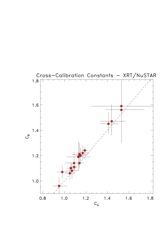
Figure 1: Plot of the cross-calibration constants between Swift/XRT and the two NuSTAR detectors (C_A and C_B).

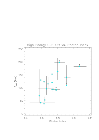
Figure 2: High energy cut-off vs. photon index (values form the spectral fit reported here; see text for details).

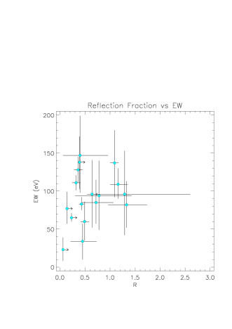
Figure 3: Plot of the EW vs reflection fraction (see table for values of the spectral fits).

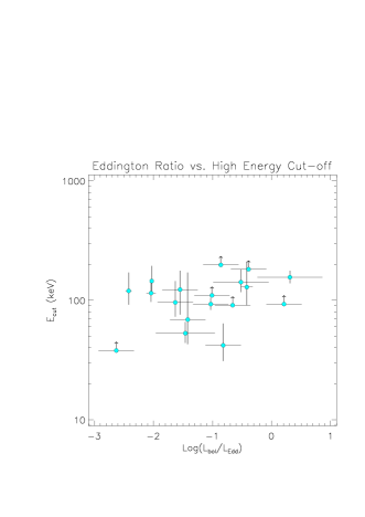
Figure 4: High energy cut-off vs. Eddington Ratio for the sources analysed here.

Given previous evidence for the decrease of the cut-off energy with increasing Eddington ratio (Ricci et al., 2018), we have also searched for a correlation between these two parameters. Table 3 reports for each source in the sample, the 2-10 keV absorption corrected luminosity and the bolometric luminosity obtained by applying the correction of Marconi et al. (2003), the most accurate black hole mass found in the literature (see last column of Table 3) and the corresponding Eddington luminosity. The Eddington ratio $\lambda$=L_bol/L_Edd is also listed with its relative uncertainty derived from the errors on the black hole mass and 2-10 keV luminosity measurements. Figure 4 shows the high energy cut-off plotted against the Eddington ratios for all the sources in the sample. We tested for a possible correlation between the two quantities by applying a Pearson statistical test, but found none, being the correlation coefficient 0.34.

Finally, we have also considered the position of our sources in the compactness versus temperature plane as discussed in Fabian et al. (2015, 2017) and have found that all sources lie in the region allowed by the pair thermostat. To transform the cut-off energy into the coronal temperature kT_e we have used a factor of 2. i.e. kT_e=E_cut/2, appropriate if $\tau$ (optical depth) is lower than 1 (see Petrucci et al. (2001)). Within this assumption, kT_e ranges from 20 keV to 80 keV. However some sources, like IGR J16119-6036, 2E 1853.7+1534 and GRS 1734-292 have temperatures which are too low to be compatible with a pure thermal plasma, introducing the need for a hybrid plasma where a non-thermal component, which tends to lower the limiting temperature, becomes significant (Fabian et al. 2017). Particularly in these cases, simultaneous XMM/NuSTAR observations would be helpful in confirming these low kT_e values, which would test the current models for a hybrid plasma.

Table 3 - Accretion Parameters
Source	Log(L2-10keV)	Log(L${}_{\rm\bf Bol}^{\rm\bf corr}$)	Log(LEdd)	Log($\bf\lambda$)	Log(MBH)	Ref.
QSO 0241+62	43.85$\pm$0.04	45.33	46.19	-0.860$\pm$0.30	8.09$\pm$0.30	Koss et al. (2017)
MCG+08-11-011	43.62$\pm$0.01	45.03	45.55	-0.520$\pm$0.47	7.45$\pm$0.47	Fausnaugh et al. (2017)
Mrk 6	42.65$\pm$0.03	43.81	46.23	-2.420$\pm$0.05	8.13$\pm$0.04	Grier et al. (2012)
FRL 1146	43.45$\pm$0.02	44.81	45.20	-0.390$\pm$0.30	7.10$\pm$0.3	($\star$)
IGR J12415-5750	43.44$\pm$0.02	44.80	46.35	-1.550$\pm$0.30	8.25$\pm$0.3	Koss et al. (2017)
4U 1344-60	43.13$\pm$0.03	44.41	$<$46.44	$>$-2.030$\pm$0.03	$<$8.34	($\star$ $\star$)
IC 4329A	43.73$\pm$0.02	45.18	44.87	0.310$\pm$0.55	6.77$\pm$0.55	Kaspi et al. (2000)
IGR J16119-6036	42.75$\pm$0.02	43.94	45.36	-1.420$\pm$0.30	7.26$\pm$0.30	Koss et al. (2017)
IGR J16482-3036	42.50$\pm$0.05	43.62	46.25	-2.630$\pm$0.30	8.15$\pm$0.30	Masetti et al. (2006)
GRS 1734-292	43.70$\pm$0.02	45.14	46.60	-1.460$\pm$0.50	8.50$\pm$0.50	Tortosa et al. (2017)
2E 1739.1-1210	43.50$\pm$0.02	44.88	45.89	-1.010$\pm$0.30	7.79$\pm$0.3	Koss et al. (2017)
IGR J18027-1455	43.75$\pm$0.02	45.20	45.86	-0.660$\pm$0.30	7.76$\pm$0.3	Koss et al. (2017)
3C 390.3	44.41$\pm$0.02	46.07	46.49	-0.420$\pm$0.10	8.39$\pm$0.10	Feng et al. (2014)
2E 1853.7+1534	44.04$\pm$0.01	45.57	46.39	-0.820$\pm$0.30	8.29$\pm$0.3	Koss et al. (2017)
NGC 6814	42.25$\pm$0.01	43.32	45.36	-2.040$\pm$0.08	7.26$\pm$0.08	Feng et al. (2014)
4C 74.26	44.86$\pm$0.01	46.67	47.70	-1.030$\pm$0.30	9.60$\pm$0.3	Koss et al. (2017)
S5 2116+81	44.31$\pm$0.02	45.94	45.73	0.210$\pm$0.30	7.63$\pm$0.3	Koss et al. (2017)
IGR J21247+5058	43.81$\pm$0.02	45.27	46.90	-1.630$\pm$0.30	8.80$\pm$0.3	Koss et al. (2017)

Notes: ($\star$): estimated from Rodriguez-Ardila et al. (2000) data, using the formula of Khorunzhev et al. (2012); ($\star$ $\star$) estimated from Masetti et al. (2006) data, using the formula of Greene & Ho (2005); if not reported in the reference paper, errors on the black hole masses have been assumed to be 0.3 dex for broad broad H_β measurements.

4 The high energy cut-off: comparison with previous works

In table 4, we report the cut-off energies obtained for the same set of sources by Malizia et al. (2014) and Ricci et al. (2017) where similar modelling of the broad-band spectra were employed, so that a straightforward comparison is possible. For completeness, we also report the cut-off energy obtained from NuSTAR data available in the literature (see table for references). Interestingly, out of 18 objects analysed in this work, only 7 have a published NuSTAR measurement on the cut-off energy; for the remaining sources, we have been able to measure for the first time a high energy cut-off in five and set upper limits in six objects.

Figure 5, left panel, shows the values of the high energy cut-off found in the present work versus the ones reported in Malizia et al. (2014). Within 2$\sigma$ errors, the values obtained from the spectral fitting of simultaneous datasets are comparable with those obtained from non-simultaneous XMM/IBIS/BAT spectra, therefore confirming these previous results. This agreement is evident in the right panel of Figure 5, where the histogram of the ratios between the high energy cut-off values measured in this work and those obtained by Malizia et al. (2014) is plotted: a clustering of these ratios is evident around 1, indicating a good match between the two studies. Finally we note that in some cases NuSTAR data allow to put more stringent constraints on the cut-off energy, while in other cases, such as those of Fairall 1146 and IGR J16482-3036, only loose constraints could be placed on the parameter, referring to Malizia et al. (2014) for a more accurate estimate of the high energy cut-off.

Figure 6, left panel, shows instead the values of the cut-off energy for the sources in our sample compared with the results reported in Ricci et al. (2017) and with previous studies performed using NuSTAR data. We note that in this case there is a lesser agreement between the high energy cut-off values measured in the two studies and a tendency for the Ricci et al. measurements to be systematically higher than what we find in the present analysis. Again this is highlighted in the right panel of Figure 6, where we plot the histogram of the ratio between the high energy cut-off values measured in this work and those obtained by Ricci et al.: in this case a similar clustering is evident, but around 0.5 indicating a systematic mismatch between the two measurements. It is worth noting that NuSTAR data employed in this work allow to put better constraints than those reported in Ricci et al. (2017) on the high energy cut-off in almost all cases, except for QSO B0241+62.

Finally, a comparison with previous NuSTAR studies of 7 sources in the sample indicates a perfect match with our results, except for the case of 4C 74.26, where the cut-off values reported in the literature (Lohfink et al., 2017) are higher than what we find in this work. Interestingly, Malizia et al. (2014) report similar values as those obtained by Lohfink et al. (2017). This source is known to host a photoionised outflow (Di Gesu & Costantini, 2016) and both Lohfink et al. (2017) and Malizia et al. (2014) took this component into account in their modelling of the source, while we were unable with the XRT data to reproduce it. Furthermore Lohfink et al. (2017) employ a different broad-band model (relxilllp) to fit the source spectrum. We have therefore re-analized our data to take into account both ionized reflection and warm absorber in the fit, but the high energy cut-off resulted always in a lower value, either in the individual observations or in their sum, in agreement with our initial analysis. We have also re-extracted the data using the same procedure details adopted by Lohfink et al. (2017), mplementing the exact same model, i.e. relxilllp but could not reproduce their results, in fact the high energy cut-off remains lower than a factor of two, but the fit is nonetheless good ($\chi^{2}$=1814 for 1800 d.o.f.; see Figure 7). At this point, the reasons behind this discrepancy are not clear.

Overall, we can conclude that our analysis confirms previous NuSTAR studies of most of our sources and furthermore indicates that a simple phenomenological model like pexrav, provides a good fit of broad-band spectra when data are not of high statistical quality. Moreover, the good match obtained comparing the present results with those of Malizia et al. (2014), strongly suggests that non simultaneity is not a major issue; this is a useful information that allows the use of good quality average spectra such as those accumulated by INTEGRAL/IBIS over a large number of AGN.

Table 4 - Previous Results
Source	Malizia et al. 2014	Ricci et al. 2017	NuSTAR (Ref)
QSO B0241+62	$>$138	177${}^{+66}_{-42}$	-
MCG+08-11-011	171${}^{+44}_{-30}$	252${}^{+131}_{-60}$	175${}^{+110}_{-50}$ (1)
Mrk 6	131${}^{+132}_{-48}$	122${}^{+42}_{-15}$	-
FRL 1146	84${}^{+79}_{-30}$	$>$72	-
IGR J12415-5750	175${}^{+296}_{-74}$	$>$229	-
4U 1344-60	$>$110	45${}^{+7}_{-4}$	-
IC 4329A	152${}^{+51}_{-32}$	236${}^{+42}_{-26}$	185${}^{+15}_{-15}$ (1)
IGR J16119-6036	$>$100	127${}^{+333}_{-64}$	-
IGR J16482-3036	163 ${}^{+220}_{-69}$	$>$90	-
GRS 1734-292	58${}^{+24}_{-7}$	84${}^{+38}_{-26}$	53${}^{+10}_{-10}$ (1)
2E 1739.1-1210	-	$>$230	-
IGR J18027-1455	$>$86	$>$74	-
3C 390.3	97${}^{+20}_{-11}$	166${}^{+64}_{-37}$	120${}^{+20}_{-20}$ (1)
2E 1853.7+1534	89${}^{+50}_{-26}$	152${}^{+413}_{-78}$	-
NGC 6814	190${}^{+185}_{-66}$	$>$210	135${}^{+70}_{-35}$ (1)
4C 74.26 (tot)	189${}^{+171}_{-66}$	$>$119	183${}^{+51}_{-35}$ (2)
S5 2116+81	$>$180	$>$175	-
IGR J21247+5058	79${}^{+23}_{-15}$	206${}^{+111}_{-27}$	100${}^{+90}_{-30}$ (3)
References: (1): Tortosa et al. (2018); (2) Lohfink et al. (2017); (3) Buisson et al. (2018).

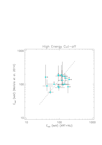
Figure 5: Left Panel: plot of the values of the high energy cut-off from the present analysis plotted against the results from Malizia et al. (2014); the 1:1 line is shown for reference. Right Panel: histogram of the ratio between the high energy cut-off values measured in this work and those obtained by Malizia et al. (2014).

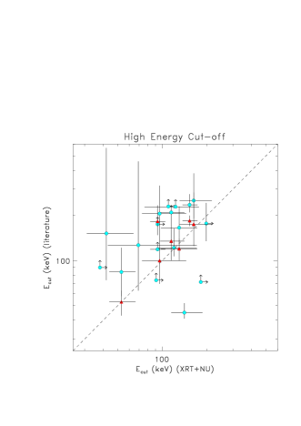
Figure 6: Left Panel: plot of the values of the high energy cut-off from the present analysis plotted against the results from Ricci et al. (2017) (cyan circles) and from several studies employing solely NuSTAR data (red triangles); the 1:1 line is shown for reference. Right Panel: histogram of the ratio between the high energy cut-off values measured in this work and those obtained by Ricci et al. (2017).

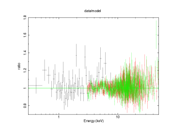
Figure 7: Data-to-model ratio for the summed observations of 4C 74.26 employing the relxilllp model, following Lohfink et al. (2017).

5 Summary and conclusions

In this work we have performed the broad-band (0.5-78 keV) spectral analysis of 18 broad line AGN, i.e. all those belonging to the INTEGRAL complete sample of AGN (Malizia et al. 2014) for which contemporaneous Swift-XRT and NuSTAR observations were available from the archives. Out of the 18 sources analysed, we found a good constraint on the high energy cut-off for 13 objects, 7 of which have already published NuSTAR measurements that we confirm in the present study; for the remaining 5 sources, we were able to place only lower limits on the value of the cut-off energy. We met the goal of our work by confirming that the distribution of the high energy cut-off in broad line AGN peaks at around 100 keV, by analysing simultaneous XRT and NuSTAR data and we also confirm what was found in our previous work (Malizia et al., 2014), which made use of non-contemporaneous XMM-Newton, INTEGRAL-IBIS and Swift-BAT spectra; we found an equally good agreement in the distribution of photon indices, for which we find a value of 1.74. This is an important result indicating that variability, if any is present, does not influence the spectral fits when dealing with high energy data obtained over long timescales as those provided by INTEGRAL-IBIS and Swift-BAT. Moreover, it is worth noting that both INTEGRAL and Swift, having accumulated long exposures on almost the whole sky, are competitive with the much more sensitive instruments on board NuSTAR whose observations typically last a few tens of ksec. In order to be able to compare these results with the old ones, we employed the same phenomenological model, pexrav, for all the sources as in 2014 and a second important result came by: using relatively simple phenomenological models over more complex and more physical ones, provides accurate measurements of the spectral parameters also with datasets of good statistical quality such as those provided by NuSTAR. A further confirmation of this is the fact that our cut-off estimates are in perfect agreement with those already published using the same NuSTAR datasets (see Table 4).

Following what was previously done by a number of other studies (e.g. Ricci et al. 2018; Tortosa et al. 2018), we have searched for correlations in our parameter space. In particular, we tested the much debated correlation between the photon index and the high energy cut-off (Perola et al., 2002): we do find a weak correlation between the two quantities, but we ascribe it to a non perfect modelisation of the low energy data due to the poor statistical quality of the XRT spectra. We also tested for a possible correlation between the high energy cut-off and the Eddington ratio, but contrary to what found by Ricci et al. (2018) and in agreement with what reported by Tortosa et al. (2018), we do not observe any.

In conclusion, the present study strongly supports the evidence that the high energy cut-off is low and located around 100 keV, using both simultaneous and non-simultaneous data, and employing either physical or phenomenological models. Clearly, to test theoretical predictions on the physical characteristics of the X-ray emitting plasma in the corona and its relation with the properties of the accreting SMBH, high statistical quality broad band data such as those provided by XMM-Newton in combination with NuSTAR and/or INTEGRAL-IBIS/Swift-BAT are essential.

Appendix A

in Figures 8, 9 and 10 are reported the best fit models together with the model-to-data ratio for the sources analysed in the sample. As described in text, we employed the pexrav model in all sources plus any other component (such as the iron Gaussian line or intrinsic absorption) as required by the data. In Figure 11 we report, as an example the confidence contour plot of the high energy cut-off vs. the photon index for three of the sources in the sample, namely MCG+08-11-011, 3C 390.3 and NGC 6814.

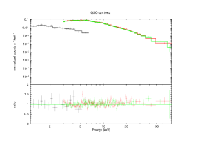
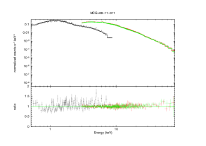
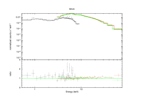
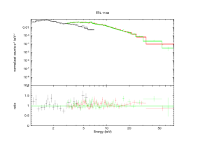
Figure 8: Data and folded model (upper panels) and model-to-data ratios (lower panel) for QSO 0241+62, MCG+08-11-011, Mrk 6, FRL 1146, IGR J12415-5750, 4U 1344-60, IC 4329A and IGR J16119-6036. Fit results are reported in Table 2.

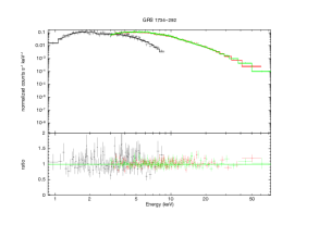
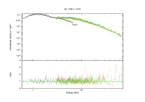
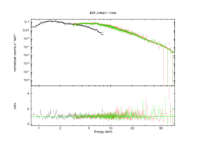
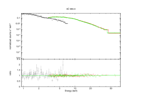
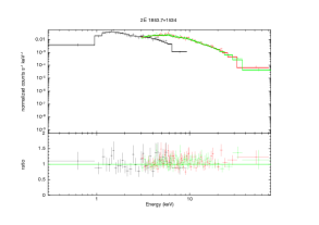
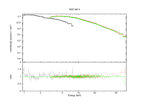
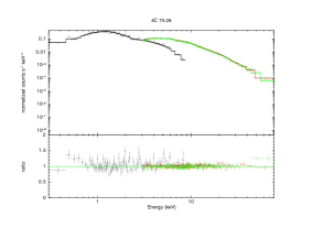
Figure 9: Data and folded model (upper panels) and model-to-data ratios (lower panel) for IGR J16482-3036, GRS 1734-292,2E 1739.1-1210, IGR J18027-1455, 3C 390.3, 2E 1853.7+1534, NGC 6814 and 4C 74.26 (summed observations). Fit results are reported in Table 2.

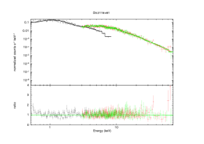
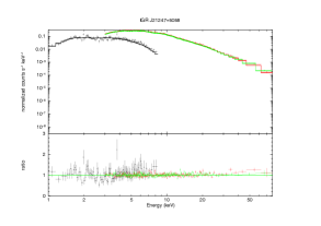
Figure 10: Data and folded model (upper panels) and model-to-data ratios (lower panel) for S5 2116+81 and IGR J21247+5058. Fit results are reported in Table 2.

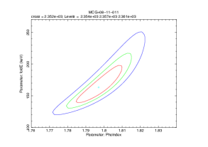
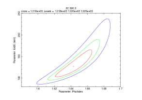
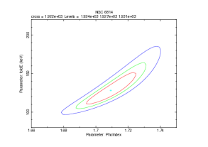
Figure 11: Confidence contour plots of the high energy cut-off vs. the photon index for MCG+08-11-011 (upper left panel), 3C 390.3 (upper right panel) and NGC 6814 (lower panel).

References

- Arnaud (1996) Arnaud K. A., 1996, in G. H. Jacoby & J. Barnes ed., Astronomical Society of the Pacific Conference Series Vol. 101, Astronomical Data Analysis Software and Systems V. p. 17
- Buisson et al. (2018) Buisson D. J. K., Fabian A. C., Lohfink A. M., 2018, MNRAS, 481, 4419
- Di Gesu & Costantini (2016) Di Gesu L., Costantini E., 2016, A&A, 594, A88
- Fabian et al. (2015) Fabian A. C., Lohfink A., Kara E., Parker M. L., Vasudevan R., Reynolds C. S., 2015, MNRAS, 451, 4375
- Fabian et al. (2017) Fabian A. C., Lohfink A., Belmont R., Malzac J., Coppi P., 2017, MNRAS, 467, 2566
- Fausnaugh et al. (2017) Fausnaugh M. M., et al., 2017, ApJ, 840, 97
- Feng et al. (2014) Feng H., Shen Y., Li H., 2014, ApJ, 794, 77
- Gilli et al. (2007) Gilli R., Comastri A., Hasinger G., 2007, A&A, 463, 79
- Greene & Ho (2005) Greene J. E., Ho L. C., 2005, ApJ, 630, 122
- Grier et al. (2012) Grier C. J., et al., 2012, ApJ, 755, 60
- Kalberla et al. (2005) Kalberla P. M. W., Burton W. B., Hartmann D., Arnal E. M., Bajaja E., Morras R., Pöppel W. G. L., 2005, A&A, 440, 775
- Kaspi et al. (2000) Kaspi S., Smith P. S., Netzer H., Maoz D., Jannuzi B. T., Giveon U., 2000, ApJ, 533, 631
- Khorunzhev et al. (2012) Khorunzhev G. A., Sazonov S. Y., Burenin R. A., Tkachenko A. Y., 2012, Astronomy Letters, 38, 475
- Koss et al. (2017) Koss M., et al., 2017, ApJ, 850, 74
- Landi et al. (2010) Landi R., Bassani L., Malizia A., Stephen J. B., Bazzano A., Fiocchi M., Bird A. J., 2010, MNRAS, 403, 945
- Lohfink et al. (2017) Lohfink A. M., et al., 2017, ApJ, 841, 80
- Lubinski & Zdziarski (2001) Lubinski P., Zdziarski A. A., 2001, MNRAS, 323, L37
- Magdziarz & Zdziarski (1995) Magdziarz P., Zdziarski A. A., 1995, MNRAS, 273, 837
- Malizia et al. (2014) Malizia A., Molina M., Bassani L., Stephen J. B., Bazzano A., Ubertini P., Bird A. J., 2014, ApJ, 782, L25
- Masetti et al. (2006) Masetti N., et al., 2006, A&A, 448, 547
- Molina et al. (2009) Molina M., et al., 2009, MNRAS, 399, 1293
- Perola et al. (2002) Perola G. C., Matt G., Cappi M., Fiore F., Guainazzi M., Maraschi L., Petrucci P. O., Piro L., 2002, A&A, 389, 802
- Petrucci et al. (2001) Petrucci P. O., et al., 2001, ApJ, 556, 716
- Ricci et al. (2017) Ricci C., et al., 2017, ApJS, 233, 17
- Ricci et al. (2018) Ricci C., et al., 2018, MNRAS, 480, 1819
- Rodriguez-Ardila et al. (2000) Rodriguez-Ardila A., Pastoriza M. G., Donzelli C. J., 2000, ApJS, 126, 63
- Tortosa et al. (2017) Tortosa A., et al., 2017, MNRAS, 466, 4193
- Tortosa et al. (2018) Tortosa A., Bianchi S., Marinucci A., Matt G., Petrucci P. O., 2018, A&AS, 614, A37