Accurate predictions for t-channel single top-quark production

Rikkert Frederix

Physik Department T31, Technische Universität München, James-Franck-Str. 1, D-85748 Garching, Germany

Single top-quark production through the exchange of a t-channel W-boson is the main electroweak production mode for top quarks at the Large Hadron Collider. I discuss a recent development in the theoretical predictions for this process, in which t-channel single-top with an additional jet is combined, at NLO accuracy, with t-channel single top production, without the introduction of a merging scale.

PRESENTED AT

$11^{\mathrm{th}}$ International Workshop on Top Quark Physics
Bad Neuenahr, Germany, September 16–21, 2018

1 Introduction

At the Large Hadron Collider (LHC) running at 13 TeV, the second largest production mode for top quarks is t-channel single-top quark production, being close to one third of the pair production mode [1, 2, 3, 4]. At variance with the pair production mode, which is governed by the strong interaction, t-channel single-top production is mediated by a W-boson and is therefore an electroweak (EW) process. This make it sensitive to a different class of new physics scenarios [5, 6, 7, 8, 9, 10] and directly sensitive to the CKM matrix element $|V_{tb}|$ [11, 12, 13, 14].

Within the Standard Model, this process is known at the next-to-leading order (NLO) in the strong coupling for a long time [15, 16, 17, 18, 19, 20] and recently also the next-to-NLO corrections have been computed [21, 22, 23]. Beyond fixed-order perturbation theory, effects from all order resummation have been studied as well [24, 25, 26]. For the Monte-Carlo simulation of completely exclusive predictions, the NLO corrections have been matched to parton showers [27, 28, 29, 30, 31, 32, 33, 34] and these NLOPS predictions are what is currently being used by the experimental collaborations to simulate the single-top process. Finally, also the NLO corrections in the EW have been considered in refs. [35, 36, 37].

While the NLOPS predictions have a remarkable accuracy, for single-top production they do not include the latest developments regarding multi-jet merging [38, 39, 40, 41, 42, 43, 44, 45, 46, 47, 48]. The results presented here, which are based on ref. [49], show that this limitation has now been lifted.

2 Method

The method used to combine NLO single-top together with NLO single-top plus jet production is the MINLO procedure [39] together with (improved and refined) ideas presented in ref. [47] to recover the NLO accuracy of the lowest multiplicity single-top process.

The MINLO method starts from a fixed-order NLO computation for single-top plus jet production, $d\sigma_{{\scriptscriptstyle\mathrm{NLO}}}^{{\scriptscriptstyle\mathrm{STJ}}}$. This process was implemented in the POWHEG BOX framework [50, 51] as the STJ generator [49] using matrix elements generated with Madgraph4 and MadGraph5_aMC@NLO [52, 53]. The single-top plus jet calculation is not reliable for observables that are inclusive over the extra jet; indeed, a strict fixed-order prediction will result to an infinitely large cross section when the energy or transverse momentum of the extra radiation approaches zero. Indeed, in this limit the cross section will be dominated by logarithms of the differential jet rate, $\sqrt{y_{{\scriptscriptstyle 12}}}$, over the hard scale of the process. To cure this infinity a simple all-order resummation is added (at leading logarithmic accuracy). Schematically this results in the MINLO cross section being defined as

$$d\sigma_{{\scriptscriptstyle\mathcal{M}}}=\Delta(y_{{\scriptscriptstyle 12}})\,\left[\,d\sigma_{{\scriptscriptstyle\mathrm{NLO}}}^{{\scriptscriptstyle\mathrm{STJ}}}-\left.\Delta(y_{{\scriptscriptstyle 12}})\right|_{\overline{\alpha}_{{\scriptscriptstyle\mathrm{S}}}}\,d\sigma_{{\scriptscriptstyle\mathrm{LO}}}^{{\scriptscriptstyle\mathrm{STJ}}}\,\right]\,,$$ (1)

where $\Delta(y_{{\scriptscriptstyle 12}})$ is the Sudakov form factor. The dampening of the Sudakov form factor cures the infinity, making the cross section finite even when looking inclusively over all radiation. The Sudakov form factor can be computed order-by-order in perturbation theory, in which the lowest order coefficients are universal and depend only on the flavor of the particles involved in the core process, while at higher orders more process dependent information enters. The term proportional to the $\mathcal{O}(\alpha_{S})$ expansion of the form factor, $\left.\Delta(y_{{\scriptscriptstyle 12}})\right|_{\overline{\alpha}_{{\scriptscriptstyle\mathrm{S}}}}$, is included to make the NLO expansion of the MINLO cross section identical to the original NLO single-top plus jet cross section. It can be shown [39] that by including only the universal coefficients LO accuracy for inclusive observables can be obtained:

$$\int dy_{{\scriptscriptstyle 12}}\frac{d\sigma_{{\scriptscriptstyle\mathcal{M}}}}{y_{{\scriptscriptstyle 12}}}=d\sigma_{{\scriptscriptstyle\mathrm{LO}}}^{{\scriptscriptstyle\mathrm{ST}}}+\mathcal{O}(\alpha_{S}).$$ (2)

To also get the NLO terms correct, more information needs to be added to the Sudakov form factor. This can either be done by using analytic expressions [45, 54, 55] or by numerical fits [47, 49] for the higher order corrections that enter the Sudakov form factor. For the t-channel single-top process it is the latter approach that has been pursued.

Fitting procedure

In order to improve the agreement in eq. (2) to NLO accuracy, we state that the following must hold

$$\frac{d\sigma_{{\scriptscriptstyle\mathrm{NLO}}}^{{\scriptscriptstyle\mathrm{ST}}}}{d\Phi}\,=\,\int dy_{12}\,\frac{d\sigma_{{\scriptscriptstyle\mathcal{M}}}}{d\Phi dy_{12}}\,\delta\Delta(y_{12})\,,$$ (3)

where $\delta\Delta(y_{12})$ is the modification needed to the original Sudakov form factor and has the form

$$\ln\delta\Delta(y_{12})\,=\,-2\int_{y_{12}}^{Q_{bt}^{2}}\frac{dq^{2}}{q^{2}}\,\overline{\alpha}_{{\scriptscriptstyle\mathrm{S}}}^{2}\,\mathcal{A}_{2}(\Phi)\,\ln\frac{Q_{bt}^{2}}{q^{2}}\,.$$ (4)

The $\mathcal{A}_{2}(\Phi)$ is an unknown function of $\mathcal{O}(1)$ that we need to obtain by imposing the equality in eq. (3) numerically. $\Phi$ is the complete Born phase-space and is therefore four-dimensional. However, one dimension is trivial (rotation about the collision axis), hence there remains a three-dimensional fit to be done. At the most basic level, in order to achieve our accuracy goal, the only requirement that need be satisfied by the modifications indicated in eqs. (3) and (4), is that $\mathcal{A}_{2}(\Phi)$ be $\mathcal{O}(1)$; this is demonstrated formally, and numerically, in ref. [49]. Since we do not want to introduce a functional bias and the function to fit is inside an exponent, we train an artificial neural network to form $\mathcal{A}_{2}(\Phi)$ that minimizes the following loss function

$$\mathcal{L}\,\,=\,\,\sum_{i=1}^{N_{\rm bins}}\,\left[\,\sum_{j=1}^{N}\,w^{\scriptscriptstyle{\rm ST}}_{i,j}\,-\,\sum_{k=1}^{N^{\prime}}\,w^{\scriptscriptstyle{\rm STJ}}_{i,k}\,\mathrm{e}^{\,\tilde{\mathcal{A}_{2}}(\Phi_{i})\,\mathcal{G}_{2}(\lambda)}\,\right]^{2}$$ (5)

after having discretized the phase-space in $N_{\rm bins}$ bins. $N$ ($N^{\prime}$) is the number of ST (STJ) events used in carrying out the fit. $w^{\scriptscriptstyle{\rm ST(J)}}_{i,j}$ is the weight of the $j$th ST(J) event in bin $i$ of the discretized Born variable parameter space. $\tilde{\mathcal{A}_{2}}(\Phi)$ is the neural network prediction for the desired effective Sudakov form factor coefficient (and $\mathcal{G}_{2}(\lambda)$ a known function). A meta-search was carried to find the optimal network architecture and using 25 million ST events and 18 million STJ events the 42 independent parameters of the resulting network where fitted. It was found that the model prediction for $\tilde{\mathcal{A}_{2}}(\Phi)$ is of $\mathcal{O}(1)$ (or smaller) all over the phase-space (as it must be for the procedure to be reliable), apart from some extreme corners where somewhat larger values where found, possibly due to a lack of statistics in the fitting procedure. The obtained model has been made available as part of the STJ generator in the POWHEG BOX.

3 Results

In the following we discuss a limited set of results that validate the new STJ^⋆ predictions. For this, we compare it to the existing ST generator [30], as well as the new STJ generator [49]. The latter includes the MINLO procedure, but without the non-universal, numerically fitted coefficients in the Sudakov form factor that make the STJ^⋆ prediction NLO accurate for ST observables, i.e., with $\delta\Delta(y_{12})=0$. The events have been generated for the 13 TeV LHC, using NNLO NNPDF3.0 parton distributions [56] and a top mass of 172.5 GeV. The events have been showered with Pythia8 [57], including the alternative momentum reshuffling for initial-final QCD dipoles [58]. The top quarks are kept stable throughout the simulation and no hadronization effects or other non-perturbative modeling have been included.

The layout of the plots is the following. In the main panel the absolute cross sections are given, with the estimates from the ST simulation in green, the STJ in blue and the best predictions, STJ^⋆ in red. The three insets display ratios of the various results to one another. The bands display the renormalization and factorization scale dependence, generated by varying the two scales independently by a factor two up and down, discarding the contributions in which the scales are varied in opposite directions. The small darker red band variation in STJ^⋆ corresponds to a factor 4 variation (up and down) of the hard scale, $Q_{bt}$, that enters the $\delta\Delta(y_{12})$ contribution, see eq. (4).

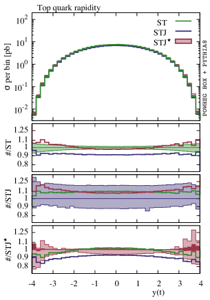
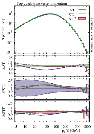
Figure 1: Predictions for the rapidity (left) and transverse momentum (right) of the top quark.

In fig. 1 the rapidity (left) and the transverse momentum (right) of the top quark are plotted. These observables are described at NLO accuracy with the ST generator, since they are inclusive over all extra radiation. For these observables the STJ calculation is only LO accurate. As expected the STJ^⋆ predictions agree within the uncertainty band with the ST predictions. This shows that including the $\delta\Delta(y_{12})$ into the STJ generator, i.e., updating it STJ^⋆, indeed recovers NLO accuracy for inclusive observables.

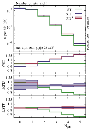
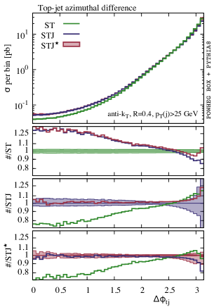
Figure 2: Predictions for the jet multiplicity (left) and azimuthal angle between the top quark and the hardest jet (right).

In fig. 2 the jet multiplicity (jets are defined with the anti-$k_{t}$ algorithm with the radius parameter set to $R=0.4$) and the azimuthal angle between the top quark and the hardest jet are shown in the left and right plots, respectively. In the left plot, it is directly obvious that where the ST generator is NLO accurate (in the 0 and 1-jet bins) the STJ^⋆ generator agrees with that predictions, while where the STJ generator is preferred, it agrees with the latter. Note that the rather small scale dependence band for the higher multiplicity bins is a well-understood artifact of the POWHEG method, that underlies all these predictions. For small values of the top quark-jet azimuthal separation (right hand plot), there must be at least one additional hard object in the event, hence this observables needs the STJ matrix elements to be NLO accurate. Indeed, the STJ^⋆ agrees with STJ in this region of phase-space. On the other hand, where the top quark and the jet are in opposite directions, the STJ and STJ^⋆ predictions start to differ, with the latter moving closer to the ST predictions. Indeed, in this region of phase space there cannot be a (single) hard object in association with the top quark and the hardest jet, hence, ST is preferred over STJ as the most accurate prediction.

4 Conclusions

The new STJ^⋆ predictions give a consistent description of ST and STJ observables at NLO accuracy. It is based on the MINLO method, but with a numerical fit for additional coefficients in the Sudakov form factor to make the STJ generator also NLO accurate for observables inclusive over the extra jet. This makes the STJ^⋆ agree STJ where STJ is NLO accurate and with ST where the latter is NLO accurate. The new STJ process, together with the numerical model to enhance it to STJ^⋆, have been made available in the POWHEG BOX framework.

Acknowledgements

I would like to thank Stefano Carrazza, Keith Hamilton and Giulia Zanderighi for the collaboration on the work presented here.

References

- [1] M. Aliev, H. Lacker, U. Langenfeld, S. Moch, P. Uwer and M. Wiedermann, Comput. Phys. Commun. 182, 1034 (2011)
- [2] P. Kant, O. M. Kind, T. Kintscher, T. Lohse, T. Martini, S. Mölbitz, P. Rieck and P. Uwer, Comput. Phys. Commun. 191, 74 (2015)
- [3] N. Kidonakis, Phys. Rev. D 82, 054018 (2010)
- [4] N. Kidonakis, arXiv:1311.0283 [hep-ph].
- [5] T. M. P. Tait and C.-P. Yuan, Phys. Rev. D 63, 014018 (2000)
- [6] Q. H. Cao, J. Wudka and C.-P. Yuan, Phys. Lett. B 658, 50 (2007)
- [7] D. Atwood, S. Bar-Shalom, G. Eilam and A. Soni, Phys. Rept. 347, 1 (2001)
- [8] E. Drueke, J. Nutter, R. Schwienhorst, N. Vignaroli, D. G. E. Walker and J. H. Yu, Phys. Rev. D 91, no. 5, 054020 (2015)
- [9] J. A. Aguilar-Saavedra, C. Degrande and S. Khatibi, Phys. Lett. B 769, 498 (2017)
- [10] C. Zhang, Phys. Rev. Lett. 116, no. 16, 162002 (2016)
- [11] J. Alwall et al., Eur. Phys. J. C 49, 791 (2007)
- [12] H. Lacker, A. Menzel, F. Spettel, D. Hirschbuhl, J. Luck, F. Maltoni, W. Wagner and M. Zaro, Eur. Phys. J. C 72, 2048 (2012)
- [13] Q. H. Cao, B. Yan, J. H. Yu and C. Zhang, Chin. Phys. C 41, no. 6, 063101 (2017)
- [14] E. Alvarez, L. Da Rold, M. Estevez and J. F. Kamenik, Phys. Rev. D 97, no. 3, 033002 (2018)
- [15] B. W. Harris, E. Laenen, L. Phaf, Z. Sullivan and S. Weinzierl, Phys. Rev. D 66, 054024 (2002)
- [16] J. M. Campbell, R. K. Ellis and F. Tramontano, Phys. Rev. D 70, 094012 (2004)
- [17] Q. H. Cao, R. Schwienhorst, J. A. Benitez, R. Brock and C.-P. Yuan, Phys. Rev. D 72, 094027 (2005)
- [18] J. M. Campbell, R. Frederix, F. Maltoni and F. Tramontano, Phys. Rev. Lett. 102, 182003 (2009)
- [19] J. M. Campbell, R. Frederix, F. Maltoni and F. Tramontano, JHEP 0910, 042 (2009)
- [20] J. M. Campbell and R. K. Ellis, J. Phys. G 42, no. 1, 015005 (2015)
- [21] M. Brucherseifer, F. Caola and K. Melnikov, Phys. Lett. B 736, 58 (2014)
- [22] E. L. Berger, J. Gao, C.-P. Yuan and H. X. Zhu, Phys. Rev. D 94, no. 7, 071501 (2016)
- [23] E. L. Berger, J. Gao and H. X. Zhu, JHEP 1711, 158 (2017)
- [24] J. Wang, C. S. Li, H. X. Zhu and J. J. Zhang, arXiv:1010.4509 [hep-ph].
- [25] N. Kidonakis, Phys. Rev. D 83, 091503 (2011)
- [26] Q. H. Cao, P. Sun, B. Yan, C.-P. Yuan and F. Yuan, Phys. Rev. D 98, no. 5, 054032 (2018)
- [27] S. Frixione, E. Laenen, P. Motylinski and B. R. Webber, JHEP 0603, 092 (2006)
- [28] S. Frixione, E. Laenen, P. Motylinski, B. R. Webber and C. D. White, JHEP 0807, 029 (2008)
- [29] R. Frederix, E. Re and P. Torrielli, JHEP 1209, 130 (2012)
- [30] S. Alioli, P. Nason, C. Oleari and E. Re, JHEP 0909, 111 (2009) Erratum: [JHEP 1002, 011 (2010)]
- [31] E. Bothmann, F. Krauss and M. Schönherr, Eur. Phys. J. C 78, no. 3, 220 (2018)
- [32] A. S. Papanastasiou, R. Frederix, S. Frixione, V. Hirschi and F. Maltoni, Phys. Lett. B 726, 223 (2013)
- [33] T. Ježo and P. Nason, JHEP 1512, 065 (2015)
- [34] R. Frederix, S. Frixione, A. S. Papanastasiou, S. Prestel and P. Torrielli, JHEP 1606, 027 (2016)
- [35] M. Beccaria, C. M. Carloni Calame, G. Macorini, E. Mirabella, F. Piccinini, F. M. Renard and C. Verzegnassi, Phys. Rev. D 77, 113018 (2008)
- [36] D. Bardin, S. Bondarenko, L. Kalinovskaya, V. Kolesnikov and W. von Schlippe, Eur. Phys. J. C 71, 1533 (2011)
- [37] R. Frederix, S. Frixione, V. Hirschi, D. Pagani, H.-S. Shao and M. Zaro, JHEP 1807, 185 (2018)
- [38] S. Alioli, K. Hamilton and E. Re, JHEP 1109, 104 (2011)
- [39] K. Hamilton, P. Nason and G. Zanderighi, JHEP 1210, 155 (2012)
- [40] S. Hoeche, F. Krauss, M. Schonherr and F. Siegert, JHEP 1304, 027 (2013)
- [41] R. Frederix and S. Frixione, JHEP 1212, 061 (2012)
- [42] S. Plätzer, JHEP 1308, 114 (2013)
- [43] S. Alioli, C. W. Bauer, C. J. Berggren, A. Hornig, F. J. Tackmann, C. K. Vermilion, J. R. Walsh and S. Zuberi, JHEP 1309, 120 (2013)
- [44] L. Lönnblad and S. Prestel, JHEP 1303, 166 (2013)
- [45] K. Hamilton, P. Nason, C. Oleari and G. Zanderighi, JHEP 1305, 082 (2013)
- [46] S. Alioli, C. W. Bauer, C. Berggren, F. J. Tackmann, J. R. Walsh and S. Zuberi, JHEP 1406, 089 (2014)
- [47] R. Frederix and K. Hamilton, JHEP 1605, 042 (2016)
- [48] J. Bellm, S. Gieseke and S. Plätzer, Eur. Phys. J. C 78, no. 3, 244 (2018)
- [49] S. Carrazza, R. Frederix, K. Hamilton and G. Zanderighi, JHEP 1809, 108 (2018)
- [50] S. Alioli, P. Nason, C. Oleari and E. Re, JHEP 1101, 095 (2011)
- [51] S. Alioli, P. Nason, C. Oleari and E. Re, JHEP 1006, 043 (2010)
- [52] J. M. Campbell, R. K. Ellis, R. Frederix, P. Nason, C. Oleari and C. Williams, JHEP 1207, 092 (2012)
- [53] J. Alwall et al., JHEP 1407, 079 (2014)
- [54] G. Luisoni, P. Nason, C. Oleari and F. Tramontano, JHEP 1310, 083 (2013)
- [55] K. Hamilton, T. Melia, P. F. Monni, E. Re and G. Zanderighi, JHEP 1609, 057 (2016)
- [56] R. D. Ball et al. [NNPDF Collaboration], JHEP 1504, 040 (2015)
- [57] T. Sjöstrand et al., Comput. Phys. Commun. 191, 159 (2015)
- [58] B. Cabouat and T. Sjöstrand, Eur. Phys. J. C 78, no. 3, 226 (2018)