KANAZAWA-19-01
Logical Reasoning
for Revealing the Critical Temperature
through Deep Learning of Configuration Ensemble
of Statistical Systems
Ken-Ichi Aoki111aoki@hep.s.kanazawa-u.ac.jp, Tatsuhiro Fujita222t_fujita@hep.s.kanazawa-u.ac.jp, and Tamao Kobayashi†333kobayasi@yonago-k.ac.jp
Institute for Theoretical Physics, Kanazawa University, Kakuma-machi, Kanazawa 920-1192, Japan
† Yonago College, National Institute of Technology, 4448 Hikona-machi, Yonago 683-8502, Japan
[Published in Journal of the Physical Society of Japan 88, 054002 (2019)]
Abstract
Recently, there have been many works on the deep learning of statistical ensembles to determine the critical temperature of a possible phase transition. We analyze the detailed structure of an optimized deep learning machine and prove the basic equalities among the optimized machine parameters and the physical quantities of the statistical system. According to these equalities, we conclude that the bias parameters of the final full connection layer record the free energy of the statistical system as a function of temperature. We confirm these equalities in one- and two-dimensional Ising spin models and actually demonstrate that the deep learning machine reveals the critical temperature of the phase transition through the second difference of bias parameters, which is equivalent to the specific heat. Our results disprove the previous works claiming that the weight parameters of the full connection might play a role of the order parameter such as the spin expectation.
1 Introduction and Summary
Recently, deep learning has been drawing attention in various applications of image recognition or artificial intelligence technology, since it has been very successful beyond expectation. In other words, why deep learning is so effective in these fields has not yet been clarified.
On the other hand, the renormalization group[4, 5, 6, 7] in physics has many common characteristics with the deep learning. The input data for the deep learning corresponds to the microvariables in physics, and the convolution filtering resembles the renormalization transformation itself, which picks up the main structural features of the input data, that is, the relevant operators (interactions) in the renormalization group terminology.[8, 9, 10, 11, 12, 13]
Therefore, analyzing these similarities between the deep learning and the renormalization group would have twofold benefits: clarifying the origin and mechanism of the effectiveness of deep learning will shed light on the strategies for improving the deep learning system and for developing new types of renormalization group.
In this work, we focus on the recent interest in the fact that the deep learning of the configuration ensemble of a statistical system may indicate the phase transition temperature of the system through the optimized machine parameters, which may behave as the order parameter of the system.[14, 15] However, there has been no logical argument or understanding of why the optimized machine parameter can possibly behave as the order parameter showing the phase transition temperature. Therefore, we analyze a deep learning machine in detail and will clarify what is learned by the machine and how it learns.
Here, we summarize our main results referring to Fig. 1, which explains the logical flow of the machine learning, its optimized parameters, and the information of physical quantities to be obtained. The machine structure is drawn schematically in Fig.2.
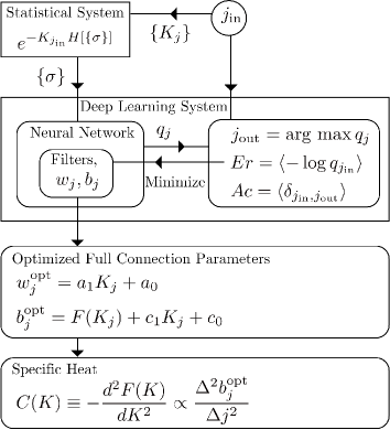
We prepare a statistical system where the physical microvariables are the spin , and denotes a configuration of the system. The statistical weight of a configuration is proportional to
| (1) |
where is the Hamiltonian of the system and is the (inverse) temperature.
We pick up an appropriate set of temperatures , where we take 16 values in this article. Taking one temperature, we make up a system configuration and transfer it to the machine with a label of temperature number . This type of learning is called supervised learning. Note that only the temperature number labels the configuration data. The actual value of does not matter at all. Furthermore, as will be clarified later, these temperatures do not have to be equally spaced or even ordered (e.g., increasing order).
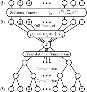
The machine receives the configuration with label as input data, which is shown in the lowest layer in Fig. 2. The target of the machine is to find the temperature number that generates the configuration. Of course, there cannot be a unique answer for the temperature of a configuration. In fact, any configuration can occur at any temperature, ignoring its actual probability of occurrence. Therefore, the machine should learn the best answer for any configuration, that is, the probabilistic correctness of the answer should be maximized.
The machine is constructed according to the standard multilayered neural network system. First, we set convolution layers, which multiply the lower layer variables by filters to make the upper layer variables. This is similar to the renormalization group transformation. Actually, we work with multiple channel filters but they are not shown in Fig. 2.
After a number of convolution layers, we average all the variables to define only one variable . This averaging policy is based on the translational invariance in the original space direction of our statistical system. Since the configurations are totally translationally invariant, the optimized machine parameters must be translationally invariant. When working with multichannel convolutional layers, they are finally summed up to make the single variable .
This intermediate variable is of essential importance. This single variable must contain sufficient information to best predict the input temperature. As proved in the next section, must be the Hamiltonian of the system (up to the normalization and origin).
Then, we set the full connection layer from to , through linear functions,
| (2) |
where is the weight and is the bias for each output channel.
Finally, we apply the softmax function to and obtain the machine output ,
| (3) |
We interpret that this is the posterior probability of temperature determined by the machine for the input configuration .
As shown in Fig. 1, we define by the maximum valued , which should be understood as the predicted temperature. If the prediction is equal to , then the case is judged as a correct answer, which totally defines the accuracy of the machine,
| (4) |
where represents the expectation value for the whole input ensembles of mixed-temperature. The machine parameters, convolution filters, and full connection parameters are optimized to lower the standard error function
| (5) |
by using the stochastic gradient descent.
The level of optimization can be evaluated by comparing the machine achievement with the theoretical bounds. In the models treated in this article, we can calculate the theoretical upper limit of the accuracy and the theoretical lower limit of the error with sufficient precision. After the numerous learnings (optimization), we retrieve the full connection parameters and .
By a simple and logical argument presented in Sec. 4, we obtain the relations that these optimized machine parameters should obey. After simple manipulation, we obtain the general solution for these optimized parameters as written in Fig. 1:
| (6) | |||||
| (7) |
where and are -independent arbitrary constants. The weight is a linear function in , and the bias is the free energy of the original statistical system up to an arbitrary linear function in . In our notation, the free energy is defined as
| (8) |
and it is a dimensionless quantity,
These relations are remarkable, which were reported first by the authors.[16] They relate the optimized machine parameters after learning with the physical quantities of the input statistical system. The first equation Eq. (6) gives us the actual temperature values up to the unit normalization () and the zero origin of the inverse temperature ().
The second equation Eq. (7) declares that the bias is simply the free energy of the statistical system at temperature up to the total normalization of the statistical weight () and the zero origin of the Hamiltonian ().
Note that the above emergence of the arbitrary constants and is inevitable, and they cannot be determined, that is, they have no physical significance here. The parameter is in general physically meaningful, but in this story of deep learning determination, it becomes irrelevant.
With these relations, we can calculate the second derivative of the free energy with respect to the temperature. The temperature spacing and order can be determined using Eq. (6). Then, the second derivative of free energy, that is, the specific heat, can be evaluated using the second-order difference of , without being disturbed by the arbitrary parameters and .
Now, the phase transition, if any and if enforcing singular peak behavior of the specific heat, is revealed through the second difference of the bias , and the critical temperature number can be read off. In the rest of this section, we apply the above summarized strategy to the two-dimensional nearest-neighbor Ising model (2d-NNI) and present the concluding plots.
We work with a -size square lattice. As the input temperatures, we take 16 values in with equal spacing (0.02) for simplicity. We plot the optimized full connection weight parameters vs or in Fig. 3, which clearly shows that is very well fitted by a linear function in .
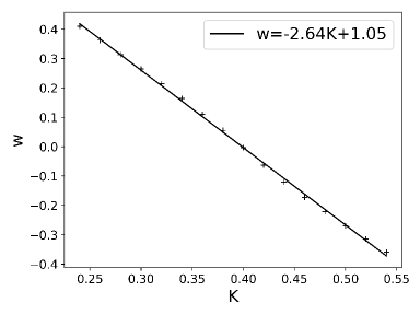
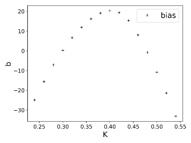
Figure 4 plots the optimized full connection bias parameters vs or . It shows that the bias is a function of with the second derivative.
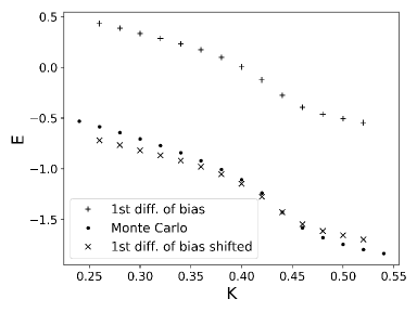
To evaluate the physical quantities, we take the first difference of , which corresponds to the energy expectation value at . In Fig. 5, we plot the first difference of compared with the exact energy expectation values obtained by Monte Carlo (MC) simulation. Also, we plot a shifted first difference of so that it is equal to the MC simulation value at . Note that the origin of the Hamiltonian has no significance here as is arbitrary. The shifted first difference of well approximates the exact energy expectation values.
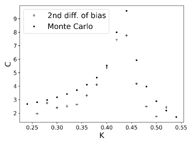
Then, we proceed to the second difference of the bias parameter, which corresponds to the specific heat. In Fig. 6, we compare the results with exact specific heat values given by MC simulation. Owing to the finiteness of our system, the specific heat does not diverge. We see the characteristic increase in the specific heat near the phase transition point (in case of the infinite volume limit).[17] Also, note that there are no remaining arbitrary constants, and the second difference of the bias quantitatively approximates the exact specific heat well. Thus, the specific heat singularity is in fact engraved in the optimized bias parameters.
These results are completely different from in statements in previously published materials[14, 15], that is, the optimized weight parameter works as an order parameter such as the spin expectation value as a function of temperature. However, these previous statements were just claimed without any logical or even plausible argument. As discussed in the next section, the single unique variable in the machine must represent the Hamiltonian as long as the machine is tuned to be optimistic. Then, the full connection weight parameter , which becomes a dimensionless quantity by being multiplied by , must have the dimensionality of the inverse energy. Actually in our solution, the weight is a linear function of and satisfies the correct dimensionality. Thus, cannot represent the spin expectation value, which is concluded even from this dimensionality argument only.
2 Optimized Machine Must Know Hamiltonian
In this section, we prove that the optimized machine must know the Hamiltonian of the system as a function of the configuration. The statistical system is defined by the statistical weight given in Eq. (1). In general, the target external control parameter is multiplied by the conjugate physical quantity in the exponent. Here, the target parameter is the inverse temperature and the conjugate is called the energy or the Hamiltonian .
The normalized probability of occurrence of a configuration is given by
| (9) |
where the partition function is defined by summing up all possible configurations,
| (10) |
We set a number of different values for the inverse temperature . In this article, we take . The total ensemble is the mixed set of configurations of the -sort of different temperatures. In this mixed-temperature ensemble, the occurrence probability of is
| (11) |
where we fix the number of configurations for each temperature to be equal.
Suppose we find a configuration , then the posterior (conditional) probability of temperature number is given by
| (12) |
Consider the machine output for the input configuration . If the machine outputs the temperature number , its accuracy, the rate of successful guesses, is simply this .
Therefore, to maximize the accuracy, the machine should output that maximizes ,
| (13) |
This is a function of and the maximum accuracy is also a function of ,
| (14) |
By averaging this with the whole input , we have the maximum value of the accuracy for the total ensemble,
| (15) | |||||
The maximum accuracy and the maximum guess are both functions of . It is important that their dependence comes only through , that is, through the Hamiltonian . We can denote this restricted dependence explicitly as
| (16) | |||
| (17) |
That is, and are functions of a single variable: the Hamiltonian of .
Now, we understand that the optimized machine to achieve the theoretical upper bound of the total accuracy must be able to correctly calculate the Hamiltonian as a function of . Also, there is no way of improving the accuracy by adding information about quantities other than the Hamiltonian. Although not literally correct, we would like to express this situation as follows: knowing the Hamiltonian is a necessary and sufficient condition for the machine to accomplish the highest limit of accuracy.
Here, we should note a subtle point. The deep learning machine is actually optimized by the condition of minimizing the error function in Eq. (5), not by maximizing the accuracy function in Eq. (4). Minimizing the error function is a much stronger condition than maximizing the accuracy. This fact can be understood quickly by looking at Fig. 24, which will be explained later in Sec. 8. In fact, the minimized error machine necessarily achieves the highest accuracy, but the reverse does not hold. In this sense, the above statement of the necessary and sufficient condition of knowing the Hamiltonian should apply rather to the minimum error machine. However, if we prepare an initial set of temperatures so that the spacing between neighboring temperatures is sufficiently small, then the difference between these two types of machines will decrease and finally vanish in the limit of infinitesimal temperature discrimination.
We extend the above argument to the case where there exist other external control parameters in the statistical weight. For example, we consider the uniform external magnetic field , which interacts with the total spin of the system . Then, the statistical weight reads
| (18) |
In fact, this statistical weight is unphysical since the interactions between the spin and the external magnetic field should be included in the Hamiltonian of the system coupled with the temperature. Of course, in the case that the Hamiltonian contains an external field parameter, there is no change in the previous conclusion, that is, the Hamiltonian function including external field interactions must be learned by the machine.
However, as a purely theoretical system, we can make an ensemble of the above type of system. Such a situation occurs in the case of the spontaneous symmetry breakdown (spontaneous magnetization), where we need a virtual external field to stabilize the system ensemble. Then, we should reconsider this case here.
First of all, the occurrence probability of for the temperature and external field is given by
| (19) |
The normalization factor also depends on the external field . In the mixed-temperature ensemble, the posterior probability of the labeled temperature is
| (20) |
Therefore, both the maximum accuracy and the guessed temperature ensuring it depend on the external field , and the total theoretical upper limit of the accuracy depends on .
Now, we look at the dependence of these quantities by substituting Eq. (19) into Eq. (20). The dependence through the total spin function cancels out between the numerator and the denominator, and only the dependence through the Hamiltonian survives,
| (21) | |||
| (22) |
We reach the same conclusion again. Even in the case where the temperature-independent external field also controls the statistical weights, the previous conclusion holds, that is, knowing the Hamiltonian is the necessary and sufficient condition for making the best available machine.
Note here that what is observed by the optimized machine does not have to be the Hamiltonian itself. Consider a procedure that the machine observes a physical quantity , obtains a value of it, , and guesses the input temperature as a function of . If all states having the same value of give a single value of the Hamiltonian, then the observation of is equivalent to that of the Hamiltonian. In other words, this case ensures the existence of a map . Therefore, the observation of such can also achieve the highest accuracy.
3 Characteristics of Optimized Machine
In this section, we investigate the optimization condition of the deep learning machine to minimize the error function in Eq. (5).
Let us recall the deep learning machine structure drawn in Fig. 2. Our machine, just before the final output stage, prepares a single variable by manipulating the input spin configuration through multiple convolutional layers.
From the discussion in the previous section, the optimized machine should know the Hamiltonian as a function of . With this structured machine, the variable is the unique variable gathering characteristic information contained in the input . Therefore, the variable must necessarily be the Hamiltonian itself of the input configuration, , so that the machine can achieve the highest accuracy and the lowest error. Hereafter, for the perfectly optimized machine, we suppose that the variable represents the Hamiltonian itself.
As mentioned in the previous section, the optimized machine should know the Hamiltonian or its equivalent , as long as there is a map from to , to achieve the highest ability. Therefore, the key variable does not have to be the Hamiltonian itself and it can be something else. However, in later sections, we confirm that, actually, the variable is optimized to represent the Hamiltonian itself up to the origin and the unit normalization. This is due to the structure of the final output layers and the optimization procedure of our machines, that is, the full connection layer with linear functions in is coupled to the softmax function output and they are optimized to minimize the error function discussed below, which is a much stronger condition than that bringing the highest accuracy.
Using this variable , the machine makes the output , by using the full connection layer and the softmax function. First, 16 variables are set by the machine as defined in Eq. (2),
| (23) |
where weight and bias are the machine parameters to be optimized in this full connection layer.
Then, these variables are transformed into via the softmax function as in Eq. (3),
| (24) |
These values are the final machine output, which are interpreted as the machine estimate of the normalized posterior probabilities of input temperature as a function of input .
Before discussing the optimization condition, we recapitulate the basic notions of evaluating the difference between two independent probability functions. We take two probability functions and , both of which are normalized,
| (25) |
We introduce the Kullback – Leibler (KL)[18] divergence to represent the size of the difference between these two probability functions,
| (26) |
In fact, the KL divergence is straightforwardly proved to be non-negative,
| (27) |
and the equality above is satisfied only at , which is the unique minimum.
We evaluate the machine by comparing the machine estimate of the posterior probabilities with the correct posterior probabilities predetermined by the input mixed temperature ensemble. The predetermined posterior probabilities are defined in Eq. (12). Then, the KL divergence comparing this and the machine estimate for a fixed is given by
| (28) |
where the machine estimate is calculated for each input and we explicitly express the dependence of .
For , although it is predetermined by the input mixed-temperature ensemble, the machine should not be assumed to know it. There is a standard practical way of evaluating the KL divergence in the course of optimization. We define the error function for each input with label as
| (29) |
Averaging over the input configurations automatically sums up all the possible input temperatures and with correct probabilities of the input ensemble.
Denoting the average over the input mixed temperature ensemble by , the averaged error function
| (30) |
is rewritten as follows by separating the summation into temperature and ,
| (31) | |||||
where the KL divergence for a fixed is defined in Eq. (28).
The optimization of the machine is performed to minimize the error function by adjusting the output while is the fixed input. Owing to the non-negative condition in Eq. (27), the minimum error function is realized at
| (32) |
and the minimum value is
| (33) |
Introducing the probability function for to appear in the total mixed temperature ensemble, we have
| (34) | |||||
where is defined as
| (35) |
This is the product probability of the temperature and in the input ensemble. Therefore, the minimum error function is the Shannon entropy of the total input ensemble minus the remaining entropy ignoring the temperature information.
Here, we should mention the accuracy given by the minimum error machine. The accuracy is frequently used to evaluate the ability of a machine to discriminate the input objects. In our case, it is defined by the frequency that the predicted temperature coincides with the labeled input temperature. To obtain the highest accuracy, the machine must predict the temperature so that it maximizes as in Eq. (13),
| (36) |
This is the best result and no machine can perform better. As explained earlier, the optimized machine should output exactly equal to for all and thus it achieves the highest possible accuracy.
Finally, in this section, we clarify how we should evaluate the level of machine power, that is, how near the obtained machine is to the optimized one. One way is to compare the achieved accuracy with the theoretical highest value. However, the optimization procedure is controlled by minimizing the error function. Therefore, we should evaluate the machine performance by comparing the error function with the theoretical minimum error value obtained in Eq. (34).
The value can be evaluated by MC simulation of the system. However, if we know the free energy of the system, it can be calculated simply. The probability functions and in Eq. (34) are expressed as functions of . However, they are actually functions of the Hamiltonian only as stressed in the previous section,
| (37) |
Then, defining the probability density function ( is a value of the Hamiltonian function ), we have
| (38) |
With this expression, we can evaluate straightforwardly if we know the energy expectation value and the specific heat at every temperature. That is, we use the normal distribution approximation and replace the density function with sum of the Gaussian distributions for each temperature. Of course, this is not completely correct, but it turned out to be a practically excellent approximation in our statistical models of spins.
4 Relations between Optimized Machine Parameters and Physical Quantities
In this section, we prove the main statement of this article: the relations between the optimized machine parameters and the physical quantities of the statistical system.
As proved in the previous sections, our optimized machine must have two features as follows:
-
1.
The intermediate variable represents the Hamiltonian of the system for all .
-
2.
The output is equal to for all and .
The purpose of this section is to prove the relations declared in Eqs. (6) and (7) from these two conditions.
To make the notation simple, we denote by . Note again that in the second statement, the condition “for all ” is equivalent to “for all ” since and can be reduced to and , respectively.
First of all, we express the key variable in terms of ,
| (39) |
where and are constants. The reason for the somewhat peculiar definition here is to simplify the final formula. We have to allow freedom of the unit normalization and the origin of energy. These two constants are irrelevant for physics and, in fact, the machine can become perfect with these uncertain arbitrary parameters. This means that the optimized machine parameters have completely flat directions for the error function.
The full connection layer sets the variable defined in Eq. (2). The final output has the relative ratio
| (40) |
where the proportionality means that as the -space vector (16-dimensional), the left-hand-side vector is proportional to the right-hand-side vector. Next, the predetermined probability defined in Eq. (12) satisfies
| (41) |
Then, the second statement is simply the following proportionality,
| (42) |
The proportionality factor can depend on and we obtain the equality
| (43) |
Taking the logarithm of both sides of this equality, we have
| (44) |
where is the free energy defined by
| (45) |
The -dependent proportionality factor is restricted. Since the above equality holds for any , must be a linear function in . We take the following notation:
| (46) |
where we introduced additional constants and . These constants also represent the completely flat directions of the error function of the optimized machine.
Substituting defined in Eq. (39) into Eq. (44), we have two equalities,
| (47) | |||||
| (48) |
Thus, we reach the key result. The full connection layer parameters of the optimized machine can be given by this solution. This solution has four free parameters, which correspond to the completely flat directions of the error function. Of course, these four constants are totally undetermined and physically insignificant parameters.
Here, we should mention that the machine does not know the temperature value itself and just knows the temperature label . In other words, there is no way or chance to tell the machine the temperature value . However, the optimized machine learns enough to know the temperature values through up to the unit normalization and the origin. These free parameters do not affect the error function at all.
Let us explain how to calculate the physical singular behavior of the specific heat of the statistical system by using the optimized machine parameters only. First of all, we reorder the temperature label so that the weight is monotonic. The correct direction, increasing or decreasing, does not matter in this stage, which will be clarified later. Then, we calculate the difference
| (49) |
which will be proportional to the corresponding spacing of the temperatures,
| (50) |
Note that we do not assume equal spacing of the input temperatures.
Then, we evaluate the first derivative of the free energy as follows:
| (51) |
Now, we have the energy expectation value at temperature . The arbitrary constant comes from the fact that the origin of the energy cannot be determined and the arbitrary corresponds to the unit normalization. Although even the sign of is indefinite, we can fix the increasing direction of temperature so that the energy expectation values increase when the temperature increases, assuming the normality of the input statistical system.
Finally, we evaluate the second derivative of the free energy,
| (52) |
This quantity must be non-negative and equal to the specific heat of the statistical system. Therefore, we find a peaked structure around the phase transition point if any.
To summarize this section, we stress the interesting point of our results. The free energy of the statistical system is not a simple quantity to calculate. According to the definition, we need the partition function, which is usually impossible to calculate. However, the deep learning machine, looking at many configurations from a mixed-temperature ensemble and minimizing the error of predicting the input temperature label, finally engraves the free energy onto the bias parameters, even as a function of temperature. Investigating these engraves parameters, we can obtain the specific heat as a function of temperature and find the existence of a singularity related to the phase transition.
5 Spin Models to be Learned
Hereafter, we set up deep learning machines and make them learn the input temperature from input spin configurations. The spin models we use here are the two-dimensional nearest-neighbor Ising model on the square lattice (2d-NNI) and the one-dimensional long-range Ising model (1d-LRI). As before, the statistical weight is given by the Hamiltonian ,
| (53) |
and we call the temperature (actually the inverse temperature).
The 2d-NNI model is the common nearest-neighbor interaction model with the Hamiltonian
| (54) |
This model, in the infinite volume limit, has the second-order phase transition at .[17] The lattice size is the and the input temperatures are 16 classes in the period with equal spacing of . We expect that the deep learning of this finite-volume system should find the specific heat singularity remnant at the phase transition temperature. This model has an exact expression for the free energy as a function of . However, it is for an infinite-volume system, and suffers from a large difference compared with our finite-volume system. Therefore, to calculate theoretical key quantities to evaluate the deep learning machines, we need high-precision MC calculation.
The 1d-LRI model has the long-range interactions
| (55) |
where the coupling constant is defined by
| (56) |
The constant determines the damping rate of the interactions. It is known that for , there is a phase transition[19, 20, 21, 22] at finite . This model is the most primitive model of quantum dissipation, which is an effective theory of the coupled harmonic oscillator system after the environmental oscillators are integrated out. In fact, the long-range interactions simply mean the nonlocal interactions in the time direction.
According to finite range scaling (FRS)[23] analysis, the phase transition point can be investigated by calculating a finite-range system where the maximum distance of interactions is limited to some number. Although such a finite-range system does not bring about any phase transition, we can extrapolate the results by increasing the maximum range to guess the infinite-range phase transition point.
Here, we set and the maximum range to be 8. We take the lattice size 1024, and the input temperatures are 16 classes in the period with equal spacing of . For , the infinite-range and infinite-volume system has a phase transition at . In this finite-range and finite-volume system, a peak of the specific heat, which is a remnant of the phase transition, is expected to appear.
This type of finite-range 1d-LRI model has a good feature. Formulating the block decimation renormalization group (BDRG),[23] we can exactly calculate the free energy as a function of temperature for any finite-volume system. Therefore, we can calculate the key quantities to evaluate machines almost exactly without relying on MC simulation. This is a major benefit compared with the 2d-NNI case.
Also, the observation of the phase transition must be more difficult in 1d-LRI than in 2d-NNI since the specific heat singularity of 1d-LRI with this size of maximum range is very much smaller than that in the 2d-NNI case. For these reasons, we take 1d-LRI with a fixed maximum range as the main model in the following sections to investigate the phase transition search by the deep learning machine as below.
6 Deep Learning Machine Details
In this section, we briefly explain the structure of the deep learning machine. We take the standard type of convolutional neural network[24, 25] with multiple layers.
The input configurations are made by MC simulation. For 1d-LRI, we have developed a new method of generating configuration data without relying on the Markov chain procedures. This new method, called exact restricted Boltzmann machine (ERBM), generates configurations with exactly zero autocorrelation. For 2d-NNI, we adopt the Wolff cluster algorithm[26] to make the ensemble stable even below the critical temperature.
In the results reported here, we do not add an external magnetic field at all. We have checked that even with an external magnetic field, all the results we claim still hold as they are.
The number of input configurations is 128,000 for 1d-LRI and 64,000 for 2d-NNI at each temperature. For 1d-LRI, we used two types of data, one is the spin configuration representing spin up or down at each site, and the other is the domain wall configuration, a dual variable representing the existence of domain walls (spin flips). The domain wall representation gives generally better results with quick convergence, and hereafter, we show the domain wall representation results.
We work with the Tensorflow software.[27] In accordance with the standard discipline, we use 80% of data for training and 20% for testing.
As explained in the previous sections, we use the error (cost) function in Eq. (5) to drive the stochastic descent optimization. Also, the accuracy is observed to check the machine quality.
We recapitulate the total machine structure in a very simple notation. We prepare the input data set and the machine makes the output data set . Our purpose is to design function ,
| (57) |
The machine consists of multiple layers and one layer converts the input data into the output data as follows:
| (58) |
where is called the activation function, is bias, and is weight. The boldface variables W, b, and x denote matrix or vector of components , , and respectively.
Building up multiple layers, we have
| (59) |
where is the layer number and . The convolutional layer is characterized through filters as
| (60) |
where is a filter of size ; the subscript is the channel component and is the stride.
By convolution, the input data of size are converted into the output data of size . At the final layer, we take the summation (average) of all variables in the direction of the space and channel,
| (61) |
where we denote this key variable by , which no longer has a suffix.
Then, we set the full connection layer and apply the softmax function. The output of the softmax function is interpreted as the probability that the input configuration belongs to the th class,
| (62) | ||||
The output is class giving the maximum probability,
| (63) |
To optimize the machine, we minimize the error function equivalent to the cross entropy,
| (64) |
where represents the configuration number and is the total number. The machine performance is also evaluated through the accuracy defined by
| (65) |
We show our typical setting of the machine parameters (hyperparameters) in Table 1. These hyperparameters are determined on the basis of experience (trial and error actually). The parameter will be explained in Sec. 7.
| hyperparameter | value |
|---|---|
| Convolution layer | layers |
| layer 1 filter size | |
| layer 1 stride | |
| other layer filter size | |
| other layer stride | |
| Mini batch size | |
| Learning rate | |
| Channel | |
| , , |
For the activation function, we use the rectified linear function (ReLU) ,
We adopt the AdamOptimizer[28] in Tensorflow for the stochastic descent method.
7 Theoretical Evaluation of Maximum Achievement
Before starting the machine learning, we calculate the theoretical limit of the accuracy and the error function so that we can be sure about the level of optimization.
The possible highest accuracy is given in Eq. (15). To understand the meaning intuitively, we start with a plot of the energy distribution for each temperature in the total ensemble.
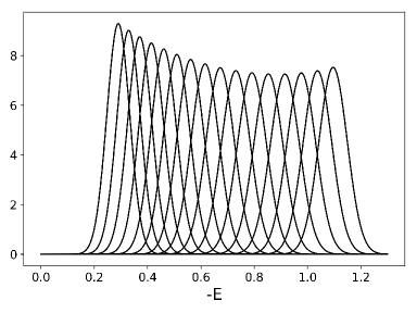
In Fig. 7, we plot the energy distribution of 16 temperatures in 1d-LRI. As noted in the previous section, we can calculate the free energy by BDRG as a function of temperature for this finite-volume system. Therefore, we obtain the energy expectation value and the energy fluctuation (specific heat) for each temperature. Using these two data, we approximate the energy distribution by the Gaussian form. This figure is plotted using this Gaussian approximation, which will be understood as sufficiently precise for our purpose.
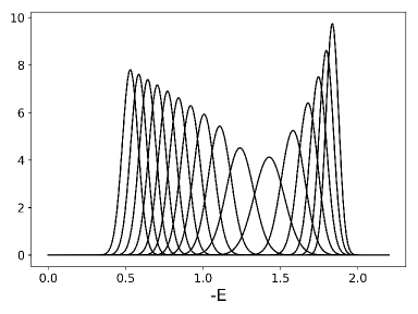
For the 2d-NNI case, we have to perform the MC simulation to calculate the energy expectation and fluctuation of a finite-volume system for each temperature. Then, using the Gaussian approximation, we plot the energy distribution in Fig. 8.
We note here that in Figs. 7 and 8, peak structures of the specific heat are already seen. Since each energy distribution is normalized, a lower peak position corresponds to a wider distribution, that is, a larger specific heat. By comparing these two figures, the 2d-NNI singularity remnant must be better recognized than that of 1d-LRI, by a human at least.
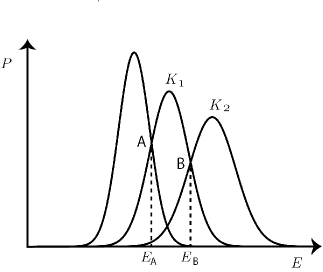
As stressed in Sec. 2, to achieve the highest accuracy, the machine should know the energy of the input configuration and then select the temperature having the largest posterior probability. In energy distribution plots, this procedure is performed as follows: calculate the energy of the input configuration, look at the energy distribution plot, and select the largest probability temperature.
In Fig. 9, we draw a schematic diagram for the logic of the maximum likelihood estimate. For the configurations whose energy is in the period , an optimized machine should output temperature since it is the maximum likelihood estimate. Among these configurations, those that are judged to output the correct answer are only those belonging to the distribution. Therefore, the total accuracy is simply the area below the upper envelope of these energy distribution lines. The overlapping region contributes to reducing the accuracy.
Thus, the best prediction changes at the crossing points of the largest distribution curves. This transition point is directly calculable. In Fig. 9, at , the two neighboring probability functions () coincide at point B,
| (66) |
Note that the number of configurations with the same energy does not depend on . Taking the logarithm of both sides, we have
| (67) |
This crossing point can be graphically understood from the plot of the free energy as a function of . Recalling that the energy expectation is given by
| (68) |
the crossing point is simply the contact point of the tangent with the slope of the line connecting the two points of the graph at and . According to the convexity of the free energy as a function of temperature, we have the inequality (we suppose )
| (69) |
Using the Gaussian approximation, we can evaluate the area below the upper envelope and find the theoretical maximum accuracy: 0.43634 (1d-LRI) and 0.51177 (2d-NNI). For 1d-LRI, we check this accuracy by alternative evaluation through the very high precision MC simulation, ERBM, and the result is 0.4364(1). This demonstrates that the Gaussian approximation is sufficiently precise for evaluating the accuracy limit.
Note that humans, and also machines, probably tend to look at the spin itself, and may count the total spin to guess the temperature. If we use the total spin to discriminate the temperature, then the maximum accuracies are only (1d-LRI) and (2d-NNI), which are much less than the above upper limit. Of course, as proved in Sec. 2, any method relying on physical quantities other than energy must decrease total accuracy.
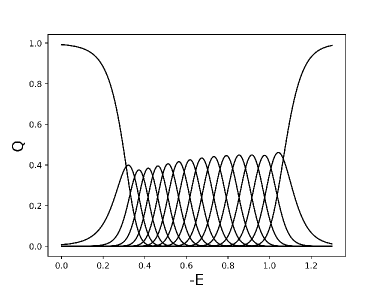
Next, we consider the minimum of the error function. As written in Eq. (38), we can calculate it directly from the energy distribution functions. In Fig. 10, the posterior probability functions are plotted for each temperature number . We integrate the entropy with the total energy probability density to obtain the minimum error. The Gaussian approximation gives (1d-LRI) and (2d-NNI). The ERBM high-precision MC simulation gives for 1d-LRI. Thus, also for the error function, the Gaussian approximation is extremely good.
The theoretical highest accuracies do not appear high. In order to make them higher, we may bundle input configurations, that is, the machine looks at configurations at once. We denote each energy of these configurations by , , and represents the configuration set number.
Then the probability of occurrence of this bundled configuration for temperature is given by the product of the probabilities of the component configurations,
| (70) | ||||
Here, we introduced the average energy for configurations,
| (71) |
We see that the average energy now controls the probability. Then the previous calculations hold by replacing the energy of the configuration with the average energy of the bundled configurations. The average energy distribution functions have the same expectation value and of the variance of the original single energy distribution. Note that the crossing point energy between distribution curves does not change by bundling. By increasing , the distribution becomes narrower and the accuracy must increase. For example, for 1d-LRI, we have the upper limits for the accuracy () and (), and the lowest errors () and (). Thus, the upper bound of the accuracy increases and the lowest error decreases markedly. This means that by using bundled multiple configurations, the amount of information becomes larger and the temperature can be discriminated more easily. However, these machines with turned out to be worse for the phase transition search, as seen later in Sec. 8.
8 Optimizing Deep Learning Machine
We analyze the optimized machine parameters. Here, we will report detailed results for the 1d-LRI case. For the 2d-NNI case, the main results are already shown in Sec. 1.
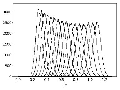
The energy distributions of the input MC configurations are plotted in Fig. 11. They reproduce well the Gaussian approximated theoretical distribution in Fig. 7.
For evidence of the level of optimization, we refer to the accuracy and the error function achieved. For 1d-LRI, after 2M iterations of learning procedures, the error function reaches below and becomes stable, which should be compared with the theoretical minimum value of . Also, the accuracy becomes above , whose theoretical upper bound is .
For 2d-NNI, after 6M iterations of learning procedures, the error function is pushed down to where the theoretical minimum is , and the accuracy becomes , where the theoretical upper limit is . From these levels of achievement, we understand that the machines are optimized very well.
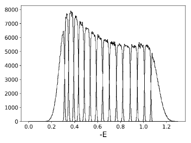
The resultant output temperatures are plotted in Fig. 12. This figure shows the energy distribution of the configurations, which are classified to each predicted temperature. The shapes of the distributions are far from Gaussian. The perfect output must show up as rectangular distributions, where the predicted temperature changes suddenly at the crossing points of energy. Since the discrimination is not perfect, there are some overlaps of distribution lines.
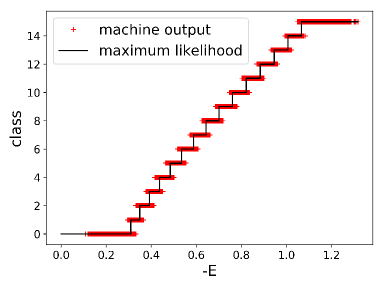
As stressed in the previous sections, to achieve high-accuracy results, we need precise energy observation of input configurations. Figure 12 shows that the energy discrimination is successful in the sense of energy blocks. This feature is also verified in Fig. 13, where we plot the relation between the output class and the energy of the configuration. The perfect machine gives a contiguous step function determined by the maximum likelihood estimate, which is drawn by a polygonal line there.
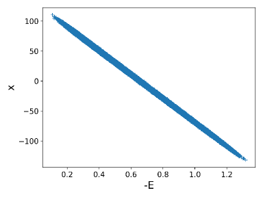
To look into the details of energy discrimination, we examine the intermediate key variable . We plot the value vs the input configuration energy in Fig. 14. This diagram shows the remarkable result that the variable is in fact organized as a linear function of the input energy. There is some broadening of the map, which causes the remaining errors.
The accuracy itself is not so high, only . However, this fact itself does not matter at all. The central issue is how near this value is to the theoretical upper limit, which can be realized only by the exact observation of the energy of the input configuration. In fact, Fig. 14 proves that the machine has learned how to evaluate the energy of input configurations. This is equivalent to the fact that the machine now knows the Hamiltonian function of the statistical system.
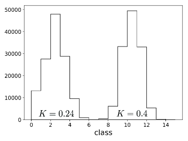
To make the above point clear, we plot the output histogram of the configurations originating from a single input temperature. Figure 15 shows the output for the input temperature and configurations.
Let us consider the implications of these histograms. The central peak of each histogram corresponds to the case that the output temperature coincides with the input temperature. The height is not so large and actually around 40% of the total histogram, which is the accuracy itself. Thus, this diagram might be interpreted to mean that the machine made mistakes for many configurations, that is, 60% of the input configurations are assigned an incorrectly predicted temperature.
Here comes the most important point of this article. We will answer the basic question about the optimized machine, that is, what is learned by the deep learning? The above statement, although it is correct, must be reinterpreted from the opposite viewpoint. That is, this diagram should be understood as the energy spectrometer outputs of the input configurations of a definite temperature. Thus, the machine becomes the energy spectrometer after learning. By supervised learning through the temperature estimate, the machine possessed an ability of the spectrometer, the analyzer of the energy. Note that the energy is chosen automatically since it is the variable conjugate to the temperature.
Now, we claim again that the low accuracy itself does not matter. The machine has learned much deeper information, the Hamiltonian of the statistical system. Now, it is time for the machine to show its obtained power.
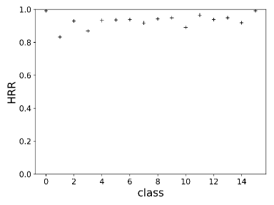
We define another characteristic to evaluate machine ability, the Hamiltonian recognition rate (HRR). Referring to Fig. 13, we define the HRR for output class by
| (72) |
where is the number of inputs whose best output temperature class is , and is the number of inputs that are on the correct step function line. In Fig. 16, we plot the HRR achieved by this machine. The total HRR,
| (73) |
is for 1d-LRI and for 2d-NNI. By evaluating the machine from this viewpoint instead of the standard accuracy value itself, we can give a better rating of the optimized machine.
Now, we examine the optimized parameters in the full connection layer. We proved in Sec. 4 that the parameters and are expected to be optimized with arbitrary linear functions of as Eqs. (47) and (48).
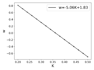
In Fig. 17, the optimized weight in the full connection layer is plotted with respect to . Here, for simplicity, we take equally spaced temperatures and the diagram axis uses instead of their label . The optimized weight is a linear function of , just as we proved in Eq. (47) for the optimized machine.
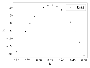
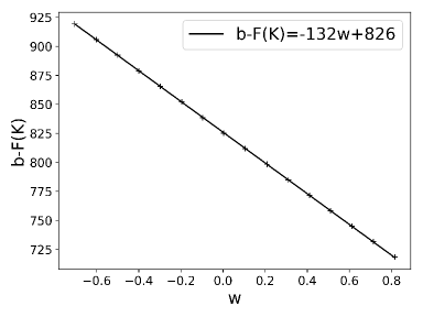
Next, we plot the optimized bias in Fig. 18. It must have a nonvanishing second derivative. According to our relation Eq. (48) proved in Sec. 4, we plot (bias minus free energy) as a function of in Fig. 19. It shows a perfectly linear function. Therefore, the optimized machine parameters satisfy the predicted formula.
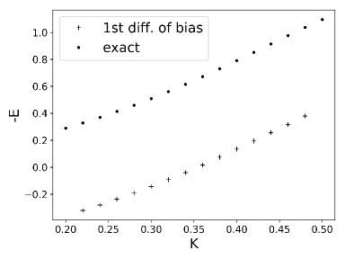
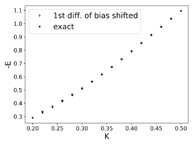
We calculate the first difference of the optimized bias according to Eq. (51) to evaluate the energy expectation value as a function of temperature. In Fig. 20, we plot the first difference and the exact values calculated by the BDRG. As is explained in Sec. 4, we see a constant shift between these two plots due to the arbitrariness of the origin of the energy. Apart from this constant shift, the coincidence is excellent, which is demonstrated in Fig. 21, where we shift the plot to coincide at .
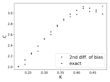
Then, we proceed to the second difference of the bias defined in Eq. (52) and plot it in Fig. 22. We also plot the exact value of this finite system calculated by BDRG. Although some statistical fluctuations remain, we can clearly see that the second difference of the bias reproduces the specific heat well quantitatively and the peak singularity appears, which is the phase transition remnant. Note that the rightmost point does not appear good, the reason for which must be the edge effect in the temperature selection. This type of edge anomaly can also be seen in Figs. 10 and 16.
Here, we add another result using the bundled configuration method introduced in Eq. (70), where we have a higher accuracy limit. The optimized machine actually achieves a higher accuracy result, , but it is somewhat low compared with the theoretical limit, , even after 2.9M learning cycles. Also the error function still remains large, , compared with the lowest limit, .
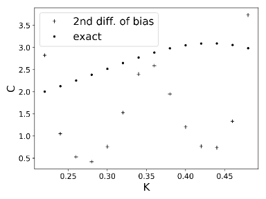
Thus, the bundled configuration learning is not effective and is not well tuned; rather, the situation is definitely worse than the single-configuration learning. We show the second difference of the bias in Fig. 23. The shape of the plot is far from the exact values, which is understandable from the error function value.
Of course, also for the bundled configuration case, the perfectly optimized machine should obey our solution as well. However, owing to the higher accuracy limit, the requirement in the machine tuning is obscurer than that in the single-configuration case, and conversely, the optimization procedure becomes subtler and harder, and the final physical output level decreases. This result is very interesting. We recall the saying that loose education does not make a person.
Now, we look at another important functions defined in the full connection layer,
| (74) |
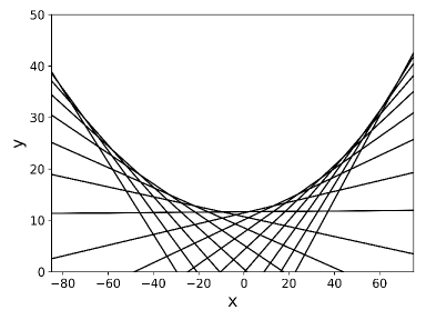
These linear functions of will be the input of the softmax function to make the final output. We plot these functions in Fig. 24. The variable represents the energy of the input configuration. We select the highest for each , which will be the maximum likelihood estimates of the temperature. We see contiguous changes of the output temperature in Fig. 24.
Now, we can understand important facts about the difference between the maximum accuracy and the minimum error conditions. The maximum accuracy can be achieved if the output temperature class obeys the step function depicted in Fig. 13. In Fig. 24, this condition is seen as follows. The crossing points of the first and second upper lines represent the stepping points of energy. Keeping the coordinate of these points the same, we can move these lines without decreasing the total accuracy. What the highest line is does matter, but the positions of other lines below it do not matter. Since we have many (17 in this case) degrees of freedom to move, there are many completely flat directions of the total accuracy in the parameter space of and .
On the other hand, we have only four arbitrary parameters for the flat directions giving the minimum error. This is because the minimum error does require complete coincidence of all output temperature posterior probabilities at any energy. Therefore, the positions of all lines at any energy do matter to ensure the minimum error. Therefore the minimum error condition is very much stronger than the maximum accuracy condition.
In Fig. 24, we also notice that an envelope function of these lines appears. As obtained in Eq. (44), the optimized machine parameter should obey the equality
| (75) |
up to a linear function in . At each point on the envelope, the value is simply the energy expectation value at the dominant temperature, . Therefore, on the envelope we can write
| (76) |
Thus, the envelope curve seen in Fig.24 represents the entropy of the statistical system as a function of energy up to a linear function in . These arbitrary parts do not contribute when we take the second derivative of the envelope curve, which also gives the specific heat again.
9 Concluding Remarks
We analyzed a simple model plant where a statistical system with a definite temperature generates configurations, which are transfered to the input data of a deep learning machine for the supervised learning of the statistical system temperature. We prepared 16 temperature classes. The temperature value itself does not matter at all here. Actually, we have no way of determining the temperature value of a physically realistic system without a verified thermometer. That is, we do not control the temperature value itself, but we just set up some equilibrium states with different temperatures by adjusting the “heating” power for the pan.
Thus, our setup of the system is totally realistic, that is, we have a statistical system that may realize a number of equilibrium states with different temperatures. There is no need for knowledge of the temperature values themselves. Even in this situation, the deep learning machine can detect the specific temperature class that corresponds to the possible phase transition point.
To evaluate objectively the level of learning or perfectness of the machine, we theoretically calculate the upper bound of the accuracy and the lower bound of the error function (cross entropy) in advance for the input configurations. The optimized machine actually gives scores that are very near to these theoretical bounds.
As proved in Sec. 2, the optimized machine must know the Hamiltonian of each configuration to realize the theoretical bound. Our machine is organized so that the input data are transformed by multilayered convolutional filtering and by averaging the space direction into the single variable . Then, this variable must be the Hamiltonian up to the origin and the unit of energy. We confirmed this property of the simple correspondence between the key variable and the energy of the input configuration as drawn in Fig. 14.
Then, the final section of the machine is a full connection layer connecting the variable and the output temperature classes through the machine parameters: weight and bias , where labels the output temperature class. The condition of minimizing the error function defined by the cross entropy is satisfied by the linear equations for and obtained in Eqs. (47) and (48).
Now, the temperature values can be read off through the weights up to the unit scaling and the origin, and as a result, is obtained as a linear function of . Then the bias is the free energy up to a linear function of . This is a remarkable result. The difference, a linear function, remains undetermined, but this is natural since it comes from the freedom of the total normalization of the partition function and the origin of the energy. These two quantities are irrelevant here, or impossible to determine by our machine learning method of analyzing the probability density of the statistical system. Then, the second derivative of free energy, the specific heat or the fluctuation of energy, is obtained without any arbitrary parameter.
The free energy is a physical quantity that has more detailed information of the statistical system than the energy itself. Its evaluation needs the information of entropy, the number of independent states with the energy fixed. Therefore, it appears somewhat miraculous that the deep learning machine engraves the free energy on its optimized bias parameters.
The key logic is that the optimization is performed to make the probability density of the energy of the machine output equal to that of the input mixed temperature set of the configurations. To evaluate the probability density, we need the entropy information or the free energy in addition to the energy, since we have to normalize them properly for each temperature. Also, the basic machine structure, that is, the key variable and the softmax function connecting it to the output temperature classes, ensures that the optimization condition can be actually satisfied, which finally records the free energy on the bias parameters.
Here, we should stress again that the above remarkable results come from the optimization condition that we adopted. Our machine is trained to minimize the cross entropy. However, the minimum cross entropy is not a necessary condition for the maximum accuracy, although it is a sufficient condition.
The reason for using the cross entropy instead of the accuracy to tune the machine parameter is simply that the stochastic steepest descent method cannot be applied to maximize the accuracy. Minimizing the cross entropy can be dealt with straightforwardly by the stochastic steepest descent. This optimization condition of the minimum cross entropy allows us to deduce our conclusion about the optimized weights and biases of the full connection section.
For the input statistical system, we adopt the one-dimensional Ising model with long-range interactions and two-dimensional Ising model with the nearest-neighbor interactions. In both models, our results of the free energy extracted from the bias parameters coincide well with the exact calculations or MC simulation results. The peak structures correctly indicate the remnant of the phase transition in both models.
Our results show that the machine trained to guess the temperature must recognize the Hamiltonian of the system, which is the conjugate variable of the temperature in the probability density function. In other words, by learning the temperature of configurations, the machine actually becomes the spectrometer of the Hamiltonian, the conjugate variable of the temperature. As stressed when explaining Fig. 15, the prediction of the temperature is just a way of learning, and actually the accuracy of prediction cannot be better than the theoretical upper limit, which is a rather low value. However, owing to the learning, the machine obtains the ability to calculate the Hamiltonian, and this ability can possibly be perfect.
We should mention here that the optimized weights and biases are simply what is memorized in the neural network as a result of learning. Therefore, we understand the total procedure as follows. By learning the temperature of each input configuration, the machine obtains the ability to evaluate the energy (conjugate of the temperature), leaving the free energy and temperature values on the neural network couplings. This is the memory newly constructed due to the learning in addition to the energy spectrometer function engraved on the lower layer parameters.
We can generalize this structure for multiple control parameters, for example, the temperature and the external magnetic field. Suppose we have control parameters and the probability density is written as
| (77) |
where is the corresponding Hamiltonian. Note that control parameters can be understood also as individual interaction coefficients, as long as they can be controlled from outside the statistical system.
We make configurations for a set of parameters and transfer them to the input configuration of the deep learning. We denote the value of set (class) by . To achieve the highest possible scores of accuracy, the deep learning machine must know all functions , which are simply the conjugate variables of . After some convolutional layers and averaging in the space direction, we must keep key variables, , which represent . The final full connection layer is defined by weight and bias as follows:
| (78) |
As before, the softmax function outputs the probability
| (79) |
Following the arguments in Sec. 4, we reach the conclusion that the optimized parameters must obey the analog of Eqs. (47) and (48),
| (80) | |||||
| (81) |
where and are arbitrary constants. Thus, the optimized machine parameters have the same characteristic structures: the weight obeys a linear function of in the direction. The second derivative of the free energy with respect to ,
| (82) |
can be evaluated without ambiguity.
We did not argue about the machine structure in detail. Actually, the simple standard form of deep learning with multilayered convolutional filtering worked well and achieved scores very near the theoretical bounds. However, it is still not perfect of course. For one-dimensional nearest-neighbor interaction case, we can easily make the perfect machine within this standard framework of the machine structure. Although the possible perfect ability of the machine to approximate any function has been argued,[29, 30, 31, 32, 33] the actual machine with a finite number of components has limited performance. As a result, we should say that our simple machine fortunately obtains a sufficiently high power so that we can observe the phase transition remnant peak of the specific heat in the second difference of the bias parameters.
We guess that the reason why such convolutional filtering succeeds in calculating the Hamiltonian is that the Hamiltonian constitutes the relatively local spin interactions. In this point, the renormalization group method of summing up local fluctuations to define effective macro-interactions should shed light on the effectiveness of the convolutional layers. However, the detailed and precise correspondence between the renormalized variables and the variables on intermediate layers has not yet been clarified. It should also be interesting to test the Hamiltonian recognition ability for various Hamiltonians including unphysical and unnatural interactions, such as long-range dominated ones.
We proved that the optimized machine must know the system Hamiltonian so that it may achieve the highest accuracy. Then, one may claim that such a machine can be trained more directly by making a function-approximating machine with supervised learning. However, note that for such supervised learning, we need the exact Hamiltonian function to label every input configuration. This is not usually the case for realistic issues. Our input label is just the temperature class used to generate the configuration. This is sufficient for the machine to learn the Hamiltonian and to engrave the free energy of the system.
The original motivation of our research was to clarify the relationship between the deep learning and the renormalization group. However, now, we notice that there exists rather large differences between the deep learning machine to learn the temperature and the renormalization group analysis, although their networking structures resemble each other closely.
The temperature is the target of deep learning, and the machine handles configurations generated by all classes of temperature simultaneously. On the other hand, for the renormalization group procedure, the temperature is the coefficient of the most relevant operators controlling the system. Strictly speaking, the relevant operator contains the Hamiltonian as its component and the temperature may play a role of labeling the size of the relevant operator.
The renormalization group describes the change of this label, the temperature parameter, as the lower layer variables are renormalized into upper layer variables. That is, the temperature changes from lower to upper layers, and it is enlarged, which means that it is relevant, while other operators are reduced to vanish and are thus called irrelevant.
We should note another apparent difference between the deep learning machine and the renormalization group. The weights and biases defining the filters in the convolutional network are optimized independently for each layer. These parameters define the upper layer variables in terms of the lower layer variables, and are simply the definition of the renormalization.
The renormalization group transformation is defined commonly for all layers. This is an essential feature of the renormalization group, that is, applying the same transformation many times. Then, after identifying the fixed point of the transformation, which corresponds to the criticality of the system, we linearize the renormalization group transformation in the neighborhood of the fixed point. Then, the transformation is characterized by its eigenvalues. Repeating the same transformation results in the enhancement and reduction of operators depending on the absolute value of their eigenvalues, which are greater than unity (relevant) or less than unity (irrelevant).
Thus, changes of the operators are described by a geometric series near the criticality. The relevant operator changes with a ratio greater than unity, and the ratio can be observed as the critical exponent through the experimental observation around criticality. This is simply the essential framework for understanding the second-order phase transition by using the renormalization group. This basic logic of the renormalization group analysis looks considerably different from the optimized machine parameter structures. However, note that this difference should not be understood as a contradiction. The optimization of the renormalization transformation independently for each step may give a new direction for the development of the renormalization group method.
Keeping these points in mind, we consider that the restricted Boltzmann machine (RBM) is expected to have tighter correspondence with the renormalization group.[9] The lower-layer visible variables are the microvariables whose probability distribution is given by the micro Hamiltonian, and the upper-layer hidden variables are regarded as the renormalized macrovariables. The weights and biases defining the RBM are simply the rules of defining the renormalization of microvariables to give the macrovariables. The upper layer macro-variables should follow the renormalized Hamiltonian. These layers can be stacked deeply similarly to the recursive renormalization group transformations.
We consider an RBM and we use the visible variables as the input configuration of the deep learning machine. We do not know the Hamiltonian controlling the visible variables. Then, can we obtain information about the Hamiltonian through the optimized deep learning machine parameters?
To learn something about the Hamiltonian, we need a set of different values of the conjugate of the Hamiltonian, the temperature. However, there is probably no simple way of adjusting the temperature with a fixed Hamiltonian by changing the RBM weight and bias parameters. The number of degrees of freedom of the Hamiltonian controlling the RBM visible variables is much larger than that of RBM machine parameters. Note that the RBM-defined Hamiltonian contains multispin interactions in addition to the basic two-spin interactions, and thus the possible number of different sorts of interactions is quite large. Therefore, we need more detailed analysis of the RBM and its effective Hamiltonians before moving forward.
Anyway, we hope that the in-depth mechanism of the high performance of the deep learning machine should be related to the mechanism of the renormalization group to treat many degrees of freedom by coarse graining and to pick up the characteristic variables automatically as relevant operators. On the other hand, we also hope that the future understanding of the origin of deep learning machine power will give us new ideas for developing the renormalization group method, which is already appreciated as a universal tool in various fields.
Acknowledgments
We acknowledge fruitful and helpful suggestions and discussions with Yasuhiro Fujii and Shin-Ichiro Kumamoto. We appreciate collaborative works of ERBM by Mariko Iijima and of MC simulation by Tsubasa Jingu, and the initial setup of our computing system and preparation studies in the early days of this project by Yuusuke Hori and Shinnosuke Onai. Also, many thanks should be given to Muneki Yasuda for his excellent lectures and for motivating us to study the relationship between the deep learning and the renormalization group.
References
- [1] [] aoki@hep.s.kanazawa-u.ac.jp
- [2] [] t_fujita@hep.s.kanazawa-u.ac.jp
- [3] [] kobayasi@yonago-k.ac.jp
- [4] K. G. Wilson, Phys. Rev. B 4, 3174 (1971).
- [5] K. G. Wilson, Phys. Rev. B 4, 3184 (1971).
- [6] K. G. Wilson and J. Kogut, Phys. Rep. 12, 75 (1974).
- [7] L. P. Kadanoff, Ann. Phys. 100, 359 (1976).
- [8] P. Mehta and D. J. Schwab, arXiv:1410.3831.
- [9] K.-I. Aoki, and T. Kobayashi, Mod. Phys. Lett. B 30, 1650401 (2016).
- [10] S. Iso, S. Shiba, and S. Yokoo, Phys. Rev. E 97, 053304 (2018).
- [11] S.-H. Li and L. Wang, Phys. Rev. Lett. 121, 260601 (2018).
- [12] S. Foreman, J. Giedt, Y. Meurice, and J. Unmuth-Yockey, EPJ Web Conf. 175, 8 (2018); Phys. Rev. E 98, 052129 (2018).
- [13] M. Koch-Janusz and Z. Ringel, arXiv:1704.06279.
- [14] A. Tanaka and A. Tomiya, J. Phys. Soc. Jpn. 86, 063001 (2017).
- [15] S. Arai, M. Ohzeki, and K. Tanaka, J. Phys. Soc. Jpn. 87, 033001 (2018).
- [16] K.-I. Aoki, T. Fujita, and T. Kobayashi, JSAI Jinkou Chinou 33, 420 (2018) [in Japanese].
- [17] L. Onsager, Phys. Rev. 65, 117 (1944).
- [18] S. Kullback and R. A. Leibler, The Annals of Mathematical Statistics 22, 79 (1951).
- [19] D. Ruelle, Comm. Math. Phys. 9, 267 (1968).
- [20] R. B. Griffiths, J. Math. Phys. 8, 478 (1967).
- [21] R. B. Griffiths, Commun. Math. Phys. 6, 121 (1967).
- [22] F. J. Dyson, Commun. Math. Phys. 12, 91 (1969).
- [23] K-I. Aoki, T. Kobayashi, and H. Tomita, Prog.Theor.Phys. 119, 509 (2008).
- [24] K. Fukushima, Biological Cybernetics 36, 193 (1980).
- [25] Y. LeCun, B. Boser, J. S. Denker, and D. Henderson, Neural Computation 1, 541 (1989).
- [26] U. Wolff, Phys. Rev. Lett. 62, 361 (1989).
- [27] M. Abadi, A. Agarwal, P. Barham, E. Brevdo, Z. Chen, C. Citro, G. S. Corrado, A. Davis, J. Dean, M. Devin, S. Ghemawat, I. Goodfellow, A. Harp, G. Irving, M. Isard, Y. Jia, R. Jozefowicz, L. Kaiser, M. Kudlur, J. Levenberg, D. Mane, R. Monga, S. Moore, D. Murray, C. Olah, M. Schuster, J. Shlens, B. Steiner, I. Sutskever, K. Talwar, P. Tucker, V. Vanhoucke, V. Vasudevan, F. Viegas, O. Vinyals, P. Warden, M. Wattenberg, M. Wicke, Y. Yu, and X. Zheng, arXiv:1603.04467.
- [28] D. P. Kingma and J. Ba, arXiv:1412.6980.
- [29] B. Irie, and S. Miyake, IEEE Int. Conf. Neural Networks 1, 641 (1988).
- [30] K. Funahashi, Neural Networks 2, 183 (1989).
- [31] K. Hornik, M. Stinchcombe, and H. White, Neural Networks 2, 359 (1989).
- [32] G. Cybenko, Mathematics of Control, Signals, and Systems 2, 303 (1989).
- [33] A. R. Barron, IEEE Transactions on Information Theory 39, 930 (1993).