Bubbleprofiler: finding the field profile and action for cosmological phase transitions

Abstract

We present BubbleProfiler, a C++ software package for finding field profiles in bubble walls and calculating the bounce action during phase transitions involving multiple scalar fields. Our code uses a recently proposed perturbative method for potentials with multiple fields and a shooting method for single field cases. BubbleProfiler is constructed with modularity, flexibility and practicality in mind. These principles extend from the input of an arbitrary potential with multiple scalar fields in various forms, through the code structure, to the testing suite. After reviewing the physics context, we describe how the methods are implemented in BubbleProfiler, provide an overview of the code structure and detail usage scenarios. We present a number of examples that serve as test cases of BubbleProfiler and comparisons to existing public codes with similar functionality. We also show a physics application of BubbleProfiler in the scalar singlet extension of the Standard Model of particle physics by calculating the action as a function of model parameters during the electroweak phase transition. BubbleProfiler completes an important link in the toolchain for studying the properties of the thermal phase transition driving baryogenesis and properties of gravitational waves in models with multiple scalar fields. The code can be obtained from: https://github.com/bubbleprofiler/bubbleprofiler.

top=2.2cm,left=3cm,right=3cm,bottom=4cm,footskip=3em

10em(.5cm) CoEPP–MN–19–1

top=2.5cm,left=3cm,right=3cm,bottom=4cm,footskip=3em

Program Summary

Program title: BubbleProfiler
Program obtainable from: https://github.com/bubbleprofiler/bubbleprofiler
Distribution format: tar.gz
Programming language: C++
Computer: Personal computer
Operating system: Tested on FreeBSD, Linux, Mac OS X
External routines: Boost library, Eigen library, GNU Scientific Library, NLopt library, GiNaC library
Typical running time: $<1$ second for single field potentials, up to O(10) seconds for potentials of several ($6+$) fields.
Nature of problem: Find the field profile in the bubble wall (bounce solution) and Euclidean action for a cosmological phase transition by solving a set of coupled differential equations.
Solution method: Direct shooting method for single field problems. Multiple field problems are solved using a perturbative algorithm which linearizes the bounce equations.
Restrictions: Currently unable to find bounce solutions for potentials of more than one fields where the vacua are nearly degenerate — these are the so-called “thin walled” cases.

Contents

1. 1 Introduction
2. 2 Quick start
   1. 2.1 Requirements
   2. 2.2 Downloading and running BubbleProfiler
3. 3 The physics problem
   1. 3.1 Thin- and thick-walled solutions
4. 4 One-dimensional shooting
   1. 4.1 Evolution with approximate solution
   2. 4.2 Evolution with Runge-Kutta
   3. 4.3 Bisection
   4. 4.4 Action
5. 5 Perturbative method for multidimensional potentials
   1. 5.1 Ansatz
   2. 5.2 Perturbative corrections
   3. 5.3 Multiple shooting method
6. 6 BubbleProfiler structure
   1. 6.1 BubbleProfiler Architecture
7. 7 Comparisons with existing codes and analytic solutions
   1. 7.1 CosmoTransitions and AnyBubble
   2. 7.2 Thin-wall
   3. 7.3 Fubini potential
   4. 7.4 Logarithmic potential
   5. 7.5 Renormalizable single-field potentials
   6. 7.6 Multi-field potentials
      1. 7.6.1 Thin walled bubbles in multi-field potentials
      2. 7.6.2 Multi-field potentials — comparison with other codes
8. 8 Scalar Singlet Model
9. 9 Conclusions
10. A Interface to bubbler solvers — bubbler
11. B Multi-field polynomial potentials
12. C Command line interface
    1. C.1 General options
    2. C.2 Ansatz options
    3. C.3 Options specific to single field direct shooting

1 Introduction

When a scalar field is in a local minimum, that is a deeper minimum of the potential exists separated from the local minimum by a barrier, the field will eventually decay to the true vacuum through quantum tunneling [1, 2, 3]. Predicting the rate of such a first order transition involves calculating the field profile for a critical bubble. This is a ubiquitous calculation in finite temperature quantum field theory and, depending on the context, requires elements of particle physics and cosmology. For example, in electroweak baryogenesis [4, 5, 6] the vacuum decays from an electroweak symmetric vacuum to a broken one via bubble nucleation. Such a scenario requires new weak scale physics to catalyze the electroweak phase transition (EWPT). This has been studied in detail for example in the minimal supersymmetric standard model (MSSM) [7, 8, 9, 10, 11, 12, 13], the next-to-MSSM [14, 15, 16, 17, 18, 19, 13, 20], as well as a variety of other Beyond the Standard Model (BSM) scenarios including multistep transitions [21, 22, 23] and effective field theory (EFT) approaches [24, 25, 26, 27, 28]. The precise behavior of the bubble nucleation can determine the efficiency of baryon production [24] as well as how quenched electroweak sphalerons are which controls the degree to which the initial baryon yield is washed out [29].

The recent discovery of gravitational waves [30] has also stirred interest in cosmic phase transitions, whether an electroweak phase transition [31, 32, 33, 34, 35, 36, 37, 38, 39, 40, 41, 42, 43], a dark sector phase transition [44, 45, 46, 47], or phase transitions motivated by some other ideas in particle physics or cosmology [48, 49, 50, 51, 52, 53, 54, 55, 56, 57, 58, 59, 60]. In all cases the properties of the relic gravitational wave spectrum are dependent on the precise details of these bubble wall profiles and how they evolve [61, 62, 63, 64, 65, 66].

The stability of the Standard Model (SM) vacuum is also a related open problem. The Higgs quartic self-coupling appears to turn negative at large scales $\mathcal{O}(10^{10}\,\text{GeV})$ when one studies its renormalization group (RG) evolution to two loops [67, 68, 69, 70, 71, 72, 73]. The precise value is subject to experimental uncertainty in the top and Higgs masses but a negative Higgs quartic implies that a catastrophic vacuum exists at very large values of the Higgs field. Whether this results in our vacuum being unstable, metastable or stable on a cosmic time scale is an outstanding theoretical and experimental problem [74] which also depends upon the maximum temperature in our cosmic history [75, 76].

Efficient publicly available codes exist for calculating the critical temperature of a phase transition [77]. However, the accurate treatment of false vacuum decay is, unfortunately, generically a numerically expensive problem. Two publicly available codes exist for calculating the decay of the false vacuum: CosmoTransitions, which is currently utilized by VEVacious [78, 79], and AnyBubble [80]. CosmoTransitions solves the bounce action using a path deformation method, while AnyBubble uses a multiple shooting method; we discuss both of these methods in more detail in Section 7. Various alternative methods for finding the bounce action have also been proposed in the literature. Since the action has a saddle point at the bounce solution, which is a maximum with respect to dilatations, Ref. [81] extremizes dilatations of the action appropriately to find the action at the bounce. The authors of Refs. [82, 83, 84] and [85] use optimization methods, by defining a minimization function that describes departures from a modified action. Refs. [86, 87] split the equation of motion into two pieces in a similar manner to the path deformation method of Ref. [78]. The authors of Refs. [86] and [88] use a gradient ascent/descent method to find the bounce. In Ref. [89] the problem is solved on a lattice. Ref. [90] connects linear solutions in Eq. 17 by approximating the potential by a polygon. Ref. [91] generalizes the single field, thin-wall case by introducing a tunneling potential that connects smoothly the false and true vacua and this method was very recently extended to the multi-field case [92]. The bounce action then is expressed as a simple integral of the tunneling potential. For the single field case, machine learning techniques are used to find the bounce in Ref. [93]. Finally, and of greatest relevance in the following, a new perturbative method was proposed in Ref. [94].

In this work we present our own easy to use bounce solver BubbleProfiler, which implements the algorithm in Ref. [94] and a direct shooting method for single field cases. We also compare and contrast BubbleProfiler with CosmoTransitions and AnyBubble. When comparing the three codes we find that BubbleProfiler is substantially faster than AnyBubble and faster than CosmoTransitions for single field cases. When calculating the tunneling action the accuracy of BubbleProfiler matches closely that of AnyBubble.

Going beyond the bounce solution to a fully-fledged calculation of the baryon yield would require solving quantum Boltzmann equations in an inhomogeneous background, which is highly non-trivial even in a toy model [95, 96]. Approximate approaches focus on CP violation from a semi-classical force [97] or the CP violation in the collision term can be estimated using the vev-insertion approach [7]. Some numerical and analytic methods have been proposed for solving the transport equations in the latter case [98, 99].

The structure of our paper is as follows. In Section 2 we provide quickstart instructions for installing and running BubbleProfiler. We describe the physical problem it solves in Section 3 and our approaches in the one-dimensional and higher-dimensional cases in Section 4 and Section 5, respectively. We present detailed information about the structure of BubbleProfiler in Section 6. We provide a detailed comparison of the results from BubbleProfiler with CosmoTransitions, AnyBubble and known analytic results in Section 7, using our bubbler interface and scripts. Finally in Section 8 we provide a quick physics application of the code, looking at bubble nucleation in the scalar singlet model, before concluding in Section 9.

2 Quick start

2.1 Requirements

Building BubbleProfiler requires the following:

• A C++11 compatible compiler (tested with g++ 4.8.5 and higher, and clang++ 3.3)

• CMake , version 2.8.12 or higher.

• The GNU Scientific Library, version 1.15 or higher.

• The NLopt library, version 2.4.1 or higher.

• GiNaC library, version 1.6.2 or higher. Note that GiNaC also requires the CLN library, which may also need to be installed separately.

• Eigen library, version 3.1.0 or higher

• Boost libraries, version 1.53.0 or higher, specifically:

  • Boost.Program_options

  • Boost.Filesystem

  • Boost.System

2.2 Downloading and running BubbleProfiler

The current release of BubbleProfiler is available as a gzipped tarball from

https://github.com/bubbleprofiler/bubbleprofiler,

or alternatively the code may be obtained using the git version control system from the same location. The documentation is hosted at

https://bubbleprofiler.github.io/.

To download and uncompress BubbleProfiler run at the command line:

⬇

$ wget https://github.com/bubbleprofiler/bubbleprofiler/archive/v1.0.0.tar.gz

$ tar -xf v1.0.0.tar.gz

BubbleProfiler uses the CMake build system generator to configure the package and generate an appropriate build system for the user’s platform. To build BubbleProfiler on a UNIX-like system with the Make build system installed as the default build tool, run at the command line:

⬇

$ cd bubbleprofiler-1.0.0

$ mkdir build

$ cd build

$ cmake ..

$ make

Note that performing an out-of-source build in a separate build directory as illustrated above is recommended, but not compulsory. The resulting library and executable are located in the lib/ and bin/ subdirectories of the main package directory, respectively.

Simple potentials can be run very quickly using the command line interface bin/run_cmd_line_potential.x executable. For example for the one-field potential,

$$V(x)=0.1\left((2-x)^{4}-14(2-x)^{2}+24(2-x)\right),$$ (1)

we can find the bounce action with the command,

⬇

bin/run_cmd_line_potential.x --potential ’0.1*((-x + 2)^4 - 14*(-x + 2)^2 + 24*(-x + 2))’ --field ’x’ --local-minimum 0.0 --global-minimum 5.0 --n-dims 3

which results in the output

⬇

Potential: 0.1*((-x + 2)^4 - 14*(-x + 2)^2 + 24*(-x + 2))

Field: x

# Action: 54.112

More details about the command line interface are given in Appendix C.

BubbleProfiler is also distributed with a suite of unit tests that may be used to check that the compiled library behaves as expected by running the command:

⬇

$ make check

Additionally, a number of small examples are provided with the downloaded package. These may be built by running:

⬇

$ make examples

The resulting example programs may be found in the bin/ directory.

3 The physics problem

The Lagrangian of a single, real scalar field is

$$\mathcal{L}=\frac{1}{2}(\partial\phi)^{2}-V(\phi).$$ (2)

Switching to Euclidean time, $t\to-\imath\tau$, we find

$$\mathcal{L}=-\frac{1}{2}(\nabla\phi)^{2}-V(\phi),$$ (3)

which leads to the equation of motion

$$\nabla^{2}\phi=V^{\prime}(\phi).$$ (4)

Assuming spherical symmetry the Laplace operator simplifies, resulting in

$$\ddot{\phi}+\frac{n}{\rho}\dot{\phi}=V^{\prime}(\phi),$$ (5)

where the dots and primes indicate derivatives with respect to $\rho$ and $\phi$, respectively. At zero temperature $n=3$ and $\rho=\sqrt{\tau^{2}+|x|^{2}}$, whereas at finite temperature $n=2$ and $\rho=|x|$ [100]. Following Ref. [1], we require that the field starts at rest,

$$\dot{\phi}(\rho=0)=0,$$ (6)

and ends at rest at the false vacuum,

$$\phi(\rho\to\infty)=\phi_{f}\quad\text{and}\quad\dot{\phi}(\rho\to\infty)=0.$$ (7)

The trivial solution, $\phi(\rho)=\phi_{f}$, is physically irrelevant as it does not describe a phase transition. We are interested in the so-called bounce action, found from the action corresponding to the Lagrangian in Eq. 3,

$$S[\phi] =\int dx^{n}d\tau\left(\frac{1}{2}\nabla\phi^{2}+V(\phi)-V(\phi_{f})\right)$$ (8)

$$=\mathcal{S}_{n}\int_{0}^{\infty}d\rho\rho^{n}\left(\frac{1}{2}\dot{\phi}^{2}+V(\phi)-V(\phi_{f})\right),$$ (9)

where the latter equality assumes a spherical symmetry and $\mathcal{S}_{n}$ is the surface area of an $n$-sphere, that is a sphere in $(n+1)$-dimensional space. The bounce is in fact a saddle-point of the action [101].

This is equivalent to a classical mechanics problem for a point-like particle moving in an upturned potential $U(q)=-V(q)$ with an unusual friction term, $n\dot{q}/t$. The equation of motion,

$$\ddot{q}+\frac{n}{t}\dot{q}=U^{\prime}(q),$$ (10)

may be found via the Euler-Lagrange method from the Lagrangian

$$L(q,\dot{q},t)=t^{n}\left(\frac{1}{2}\dot{q}^{2}-U(q)\right).$$ (11)

We must delicately tune the initial position, $q(t=0)$, such that the particle rolls down a hill and balances exactly on top of another hill. The unusual friction term falls with $1/t$. Due to the mechanical analogy, in the following we refer to the argument of the field, $\rho$, as time.

For a quadratic potential of the form

$$V(\phi)=V^{\phantom{\prime}}_{0}+V^{\prime}_{0}\phi+\frac{1}{2}m^{2}\phi^{2},$$ (12)

the exact solution for $m^{2}\neq 0$ is

$$\phi(\rho)=\frac{A}{(|m|\rho)^{p}}J_{p}\left(-\imath\sqrt{m^{2}}\rho\right)+\frac{B}{(|m|\rho)^{p}}Y_{p}\left(-\imath\sqrt{m^{2}}\rho\right)-\frac{V^{\prime}_{0}}{m^{2}},$$ (13)

where $p=(n-1)/2$, $J_{n}$ is the order $n$ Bessel function of the first kind, and $Y_{n}$ is the order $n$ Bessel function of the second kind. If, on the other hand, $m^{2}=0$, we find,

$$\phi(\rho)=A+\frac{B}{(n-1)}\frac{1}{\rho^{n-1}}+\frac{V^{\prime}_{0}}{2(n+1)}\rho^{2},$$ (14)

where the first and second terms are complementary solutions and the third term is the particular one. If $m^{2}\neq 0$, the qualitative behavior of the solution depends upon the sign of $m^{2}$. For example, in the $n=2$ case, for $m^{2}>0$ we find

$$\phi(\rho)=A\,\frac{\sinh\left(|m|\rho\right)}{|m|\rho}+B\,\frac{\cosh\left(|m|\rho\right)}{|m|\rho}-\frac{V^{\prime}_{0}}{m^{2}},$$ (15)

where for simplicity we rescaled the constants $A$ and $B$. Whereas for $m^{2}<0$,

$$\phi(\rho)=A\,\frac{\sin\left(|m|\rho\right)}{|m|\rho}+B\,\frac{\cos\left(|m|\rho\right)}{|m|\rho}-\frac{V^{\prime}_{0}}{m^{2}},$$ (16)

where we again rescaled the constants $A$ and $B$. Finally for $m^{2}=0$,

$$\phi(\rho)=A+\frac{B}{\rho}+\frac{V^{\prime}_{0}}{6}\rho^{2}.$$ (17)

We will later utilize these solutions by Taylor expanding potentials to quadratic order to match the form in Eq. 12 and applying the boundary conditions in Eq. 6 and Eq. 7.

The problem generalizes to $N$ scalar fields, in which case there are $N$ coupled second-order differential equations,

$$\ddot{\phi}_{i}+\frac{n}{\rho}\dot{\phi}_{i}=\frac{\partial V}{\partial\phi_{i}},$$ (18)

with $i=1,\ldots,N$. The general $N$-field problem is significantly more challenging than the single-field case as the bounce solution may take a curved path through the field space.

3.1 Thin- and thick-walled solutions

Bounces are characterized by the time they spend close to the true vacuum. This time-scale determines the magnitude of the action. There are two extremes: thin-walled and thick-walled bounces. Thin-walled bounces occur when the true and false vacua are nearly degenerate,

$$\frac{V(\phi_{b})-V(\phi_{f})}{V(\phi_{b})-V(\phi_{t})}\simeq 1,$$ (19)

where $\phi_{t}$ is the field value in the true vacuum and $\phi_{b}$ is the value of the field on the top of the barrier. Note that this quantity is bounded by zero and one. In this extreme, losses to friction must be minimized to ensure that there is sufficient energy to reach the false vacuum. The bounce thus sits close to the true vacuum until the time at which friction, which falls as $1/\rho$, cannot stop it reaching the false vacuum. In the thin-walled limit, the action diverges.

Thick-walled bounces, on the other hand, occur when the barrier between the true and false vacua is negligible,

$$\frac{V(\phi_{b})-V(\phi_{f})}{V(\phi_{b})-V(\phi_{t})}\simeq 0.$$ (20)

In this extreme, the initial potential energy must be similar to $V(\phi_{f})$ to ensure we do not overshoot the false vacuum. The bounce spends limited time sitting near the true vacuum. In Eq. 27 we introduce a measure of the thickness/thinness of a bounce for the one-dimensional case.

4 One-dimensional shooting

To solve the one-dimensional bounce equation, that is the bounce equation for a single field, we use a shooting method, similar to that in CosmoTransitions. We guess an initial value for the field, $\phi_{0}\equiv\phi(\rho=0)$, evolve it in time, and check whether we overshot or undershot, that is whether we started too far up the maximum and rolled beyond the next maximum or started too close to the well lying between the maxima and rolled back into it. This is illustrated in Fig. 1. It was proven in Ref. [1] that there is always at least one non-trivial solution. The argument is roughly that a friction term is dissipative,

$$\frac{dE}{d\rho}=\frac{d}{d\rho}\left(\frac{1}{2}\dot{\phi}^{2}-V(\phi)\right)=-\frac{n}{\rho}\dot{\phi}^{2}\leq 0,$$ (21)

thus we always undershoot if we begin with insufficient energy, e.g., close to the barrier. On the other hand, it can be proven by inspecting Eq. 13 that if the field starts sufficiently close to the true vacuum, it remains close to the vacuum for an arbitrary time, after which the friction term may be neglected. Thus, by energy conservation, we overshoot the true vacuum.

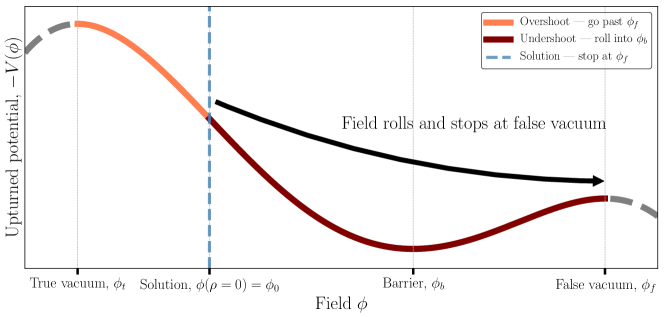
Figure 1: Illustration of shooting method for an upturned scalar potential with two minima. Beginning at rest in the orange region results in an overshot, whereas beginning in the brown region results in an undershot. We bisect between overshots and undershots until we find a solution (the blue dashed line). For the solution, the field rolls and comes to rest at the false vacuum.

4.1 Evolution with approximate solution

For small $\rho$, the friction term dominates and the field evolves extremely slowly. To avoid integrating the ODEs in this period, we first evolve the system by utilizing an approximate solution. We expand the potential about our guess of $\phi_{0}$, neglecting terms higher than quadratic,

$$V(\phi-\phi_{0})=V^{\phantom{\prime}}_{0}+V^{\prime}_{0}(\phi-\phi_{0})+\frac{1}{2}m^{2}(\phi-\phi_{0})^{2}.$$ (22)

This matches the form in Eq. 12 which is solved by Eq. 13. Using the initial condition $\phi(\rho=0)=\phi_{0}$ to fix the integration constants, we obtain, e.g., in the $n=2$ case for $m^{2}>0$,

$$\phi(\rho)-\phi_{0}\approx\frac{V^{\prime}_{0}}{m^{2}}\left[\frac{\sinh(|m|\rho)}{|m|\rho}-1\right],$$ (23)

and for $n=3$,

$$\phi(\rho)-\phi_{0}\approx\frac{V^{\prime}_{0}}{m^{2}}\left[\frac{2I_{1}(|m|\rho)}{|m|\rho}-1\right].$$ (24)

The $m^{2}=0$ cases are simply the $m^{2}\to 0$ limits of Eq. 23 and Eq. 24. Note that using the initial condition $\phi(\rho=0)=\phi_{0}$, the constants of integration in Eq. 17 must be zero.

We find the time, $\hat{\rho}$, at which the field has rolled a small fraction $f$ towards the false vacuum,

$$\left|\phi(\hat{\rho})-\phi_{0}\right|=f\left|\phi_{f}-\phi_{0}\right|,$$ (25)

where $f$ is set by Shooting::set_evolve_change_rel and has a default value of $10^{-2}$. We solve this equation using approximate analytic solutions. E.g., in the $n=2$ case we approximately invert hyperbolic sinc using

$$\operatorname{sinch}^{-1}(x)\approx\begin{cases}\sqrt{6(x-1)}&x<1.5\\ -W_{-1}(-1/(2x))&x\geq 1.5\end{cases},$$ (26)

where $W_{-1}(x)$ is the negative branch of the Lambert-$W$ function. Similarly, an approximate analytic solution is used in the $n=3$ case. Thus we solve for $\hat{\rho}$, at which we know $\phi(\hat{\rho})$ from Eq. 25, and calculate $\dot{\phi}(\hat{\rho})$ from the analytic derivative of the approximate solution. There are two problematic cases, characterized by the thinness, defined

$$t\equiv\frac{f\left|\phi_{f}-\phi_{0}\right|m^{2}}{V^{\prime}_{0}}.$$ (27)

If this quantity tends towards zero, we require a thick-wall solution and if it diverges, we require a thin-wall solution. Where necessary, we treat these cases with special asymptotic formulae. In the case of thin-walled solutions, the asymptotic formulae are functions of the logarithm of the starting distance to the true vacuum (i.e., $\lambda$, as defined in Eq. 30). This allows a numerical treatment of fine-tuned thin-wall cases. This is implemented in Shooting::evolve.

4.2 Evolution with Runge-Kutta

We take the field, $\phi(\hat{\rho})$, and velocity, $\dot{\phi}(\hat{\rho})$, and evolve them forwards in time with a controlled Runge-Kutta Dormand Prince method [102] implemented in boost. This approach means that we do not solve ODEs in the period during which friction dominates and avoid the singularity in the ODE at $\rho=0$. This is implemented in Shooting::ode.

If the field is heading back towards the true vacuum or if there is insufficient kinetic energy,

$$\frac{1}{2}\dot{\phi}^{2}<-\left(V(\phi_{f})-V(\phi)\right),$$ (28)

we consider it an undershot and return 1. If the field has passed the false vacuum, we consider it an overshot and return -1. This is implemented in Shooting::shoot.

We guess the initial step size in $\rho$ by guessing the characteristic size of the bubble,

$$\Delta\rho=\frac{2\pi}{\sqrt{-V^{\prime\prime}(\phi_{b})}}.$$ (29)

This follows from approximating the potential at the barrier by a quadratic and finding the period of oscillations. This is implemented in Shooting::bubble_scale. The initial step size is a fraction (Shooting::set_drho_frac) of this period, which is $10^{-3}$ by default.

4.3 Bisection

In Shooting::shooting, we bisect between overshots and undershots. We bisect upon the variable

$$\lambda\equiv-\ln\frac{\phi_{0}-\phi_{t}}{\phi_{b}-\phi_{t}},$$ (30)

between Shooting::bisect_lambda_max = 5 and 0, corresponding very near the true vacuum,

$$\frac{\phi_{0}-\phi_{t}}{\phi_{b}-\phi_{t}}=e^{-5},$$ (31)

and the position of the barrier, $\phi_{b}$. If Shooting::bisect_lambda_max = 5 is not an overshot, the range for the bisection is automatically shifted. We stop once a relative precision of Shooting::shoot_bisect_bits significant bits is reached. In thin-walled cases, the evolution in Section 4.1 depends only upon $\lambda$ and thus we may treat fine-tuned cases in which $\phi_{0}-\phi_{t}$ is extremely small so long as the logarithm in Eq. 30 is not so big that it cannot be represented by a double.

4.4 Action

Lastly, we calculate the action. Because we find a stationary point of the action, we know that for $\phi(a\rho)$, the action must be extremized at $a=1$. Thus we find that the contributions to the action from the kinetic term, $S_{T}$, and from the potential, $S_{V}$, are related (see e.g., Ref. [80]) through

$$S_{V}=\frac{1-n}{1+n}S_{T},$$ (32)

where

$$S_{T} =\mathcal{S}_{n}\int_{0}^{\infty}d\rho\rho^{n}\,\frac{1}{2}\dot{\phi}^{2},$$ (33)

$$S_{V} =\mathcal{S}_{n}\int_{0}^{\infty}d\rho\rho^{n}\,\left[V(\phi)-V(\phi_{f})\right].$$ (34)

Thus we may determine the action from $S_{T}$, $S_{V}$ or through a linear combination,

$$S=S_{T}+S_{V}=\frac{2}{1+n}S_{T}=\frac{2}{1-n}S_{V}.$$ (35)

We find that calculating the action from summing only the kinetic term is more accurate, especially for thick-walled solutions, and avoids evaluations of the potential, which may be computationally expensive. For the interior of the bubble wall, at $\rho\leq\hat{\rho}$, we approximate the action using analytic integration of the approximate solution in Eq. 13. We treat thin-walled cases by a special asymptotic formula.

For the bubble itself, we evolve the fields one more time from $\phi(\hat{\rho})$, this time summing the action using a trapezoid rule, with an increment $\Delta\rho$ determined by the adaptive Runge-Kutta method. We stop the evolution once we undershoot, overshoot, or arrive at the false vacuum to within a relative tolerance of Shooting::action_arrived_rel. This is implemented in Shooting::action.

The accuracy difference between calculating the kinetic and potential terms stems from the fact that summing the potential term involves a cancellation between positive and negative contributions. When the field is on top of the false vacuum, the integrand is negative. When it is in the well, it is positive. Thus, especially for thick-walled solutions that slowly roll through the well, we require a precise subtraction between the positive and negative contributions, which can be numerically challenging. The integrand of the kinetic term, on the other hand, is always positive.

5 Perturbative method for multidimensional potentials

When the potential is a function of more than one field, direct shooting is no longer possible as the enlarged space of initial conditions precludes an approach based on bisection. We instead apply the Newton-Kantorovich method [103], as discussed in Ref. [94]. In this approach, the original nonlinear problem is solved using an iterative algorithm in which successive corrections are applied to a judiciously chosen initial guess for the bounce solution. At each step of the iteration, the corrections are determined by solving a system resulting from linearizing the equations of motion, and hence are easily calculated using standard numerical methods. The iteration continues until the estimated action and values of the fields converge to within the desired tolerance. Unlike the shooting method in Section 4, this method is applicable to both the single and multi-field cases.

5.1 Ansatz

The first step in the perturbative algorithm is to construct an initial guess or ansatz for the solution. To construct this ansatz, we typically assume that the path is a straight line between the true and false vacua. On the straight line path, the potential is a one-dimensional function of the path length. We provide two options for the profile along that path, which is our ansatz, and also allow for arbitrary ansatzes:

Shooting

The most straightforward way to construct an ansatz is to solve this reduced, one-field problem using the shooting method of Section 4.

Look-up tables

A less computationally expensive option is described in Ref. [94], which proposes an analytic ansatz based on the idea that the potential between the true and false vacua can be approximated by a fourth-order polynomial. Once that is done, through reparameterizations the potential can be recast in terms of a single parameter, $\alpha$ (see Section 7.5).

The so-called kink solutions

$$\phi(\rho)\approx\phi_{0}\left[1-\tanh\left(\frac{\rho-\delta(\alpha)}{w(\alpha)}\right)-\frac{L}{w(\alpha)}\operatorname{sech}^{2}\left(\frac{\delta(\alpha)}{w(\alpha)}\right)e^{-\rho/L}\right],$$ (36)

are approximate solutions to the tunneling problem for a fourth-degree polynomial potential of the form given in Eq. 67. Here the functions $\delta(\alpha)$ and $w(\alpha)$ characterize respectively the location and width of the bubble wall. They are found by interpolation from look-up tables built from numerical fits based on solutions using the methods of Section 4. The resulting ansatz typically approximates the numerical bounce solution for the potential in Eq. 67 with an absolute discrepancy of at most $0.003$. We fix $L=1/(\phi_{f}-\phi_{t})$. Note that $\phi(\rho=0)\approx\phi_{0}$ and that we have added a term to the usual kink solution to ensure that $\dot{\phi}(\rho=0)=0$.

Text file

An arbitrary ansatz may also be provided in a text file. This may be desirable if a straight-line between the true and false vacua is a poor ansatz, regardless of the behavior along that path with respect to $\rho$. See Appendix C.2 for a description of the required file format.

5.2 Perturbative corrections

Starting from an initial ansatz constructed in the manner described above, we then proceed to compute a series of approximations $\phi_{i}^{(j)}(\rho)$ to the exact solution $\phi_{i}(\rho)$ for the $i^{\text{th}}$ field, $i=1,\ldots,N$. The $j^{\text{th}}$ iterate is given by

$$\phi_{i}^{(j)}(\rho)=\phi_{i}^{(j-1)}(\rho)+\epsilon_{i}^{(j-1)}(\rho),\quad i=1,\ldots,N,\,j=1,2,\ldots$$ (37)

where $\epsilon_{i}^{(j)}(\rho)$ denotes a correction to the previous iterate and $\phi_{i}^{(0)}(\rho)\equiv A_{i}(\rho)$. Provided that our initial guess is carefully chosen, the corrections $\epsilon_{i}^{(j)}(\rho)$ are expected to satisfy $|\epsilon_{i}^{(j)}(\rho)|\ll|\phi_{i}^{(j)}(\rho)|$ for each field $i$ and for all $\rho$.

The corrections $\epsilon_{i}^{(j)}(\rho)$ at each step of the iteration are determined by requiring that $\phi_{i}^{(j+1)}(\rho)$ should approximately satisfy the classical equations of motion. Substituting Eq. 37 into Eq. 18 and Taylor expanding the scalar potential yields

$$\frac{\partial^{2}\epsilon_{i}^{(j)}}{\partial\rho^{2}}+\frac{n}{\rho}\frac{\partial\epsilon_{i}^{(j)}}{\partial\rho}-\sum_{k}\left.\frac{\partial^{2}V(\phi)}{\partial\phi_{i}\partial\phi_{k}}\right|_{\phi^{(j)}}\epsilon_{k}^{(j)}=B_{i}^{(j)}(\rho)+O(\epsilon^{2}),$$ (38)

where the inhomogeneous terms $B_{i}^{(j)}(\rho)$ are given by

$$B_{i}^{(j)}(\rho)=\left.\frac{\partial V(\phi)}{\partial\phi_{i}}\right|_{\phi^{(j)}}-\frac{\partial^{2}\phi_{i}^{(j)}}{\partial\rho^{2}}-\frac{n}{\rho}\frac{\partial\phi_{i}^{(j)}}{\partial\rho}.$$ (39)

Upon neglecting those terms that are $O(\epsilon^{2})$ or higher, we arrive at a linear system of differential equations for the corrections $\epsilon_{i}^{(j)}$. Note that this is similar to the approach in Ref. [89], in which one Taylor expands to first order about an ansatz found by solving the bounce equation without friction. The necessary boundary conditions for the corrections are obtained by substituting the definition of $\epsilon_{i}^{(j)}$ into the boundary conditions for the fields $\phi_{i}$,

$$\epsilon_{i}^{(j)}(\rho\to\infty)={\phi_{f}}_{i}-\phi_{i}^{(j)}(\rho\to\infty),\quad\dot{\epsilon}_{i}^{(j)}(\rho=0)=-\dot{\phi}_{i}^{(j)}(\rho=0).$$ (40)

In doing this we have gained the advantage of replacing $N$ nonlinear coupled equations with $N$ linear coupled equations. The resulting linear boundary value problem may then be efficiently solved using standard numerical techniques. In particular the $N$-dimensional generalization of the shooting method described in section 18.1 of Ref. [104] is directly applicable. We review this technique in Section 5.3.

In general, the convergence of this iterative procedure to the true solution depends on the quality of our initial guess for the solution. In particular, the guess for the solution must be sufficiently accurate so that neglecting the $O(\epsilon^{2})$ terms in Eq. 38 is justified. A heuristic condition for the validity of this approach is that the missing terms are smaller in magnitude than the terms kept in the Taylor series. However, since we do not directly control the size of $\epsilon$, violations of this rule are somewhat inevitable for some values of $\epsilon(\rho)$. The violations, though, do not necessarily prevent our algorithm from reaching a bounce solution [94]. When this is not the case and a poor initial guess is responsible for a failure of the algorithm, one may of course attempt to remedy the situation by employing an alternative ansatz. Provided that the chosen ansatz satisfies a set of sufficient conditions that depend only on the particular system at hand and the initial guess itself, then the iteration is guaranteed to converge and, for a sufficiently accurate initial guess, is expected to do so with a quadratic rate of convergence [103]. We illustrate this for a typical two-field example in Figure 2. The corrections $\epsilon$ reduce with each iteration, quickly converging to a bounce solution.

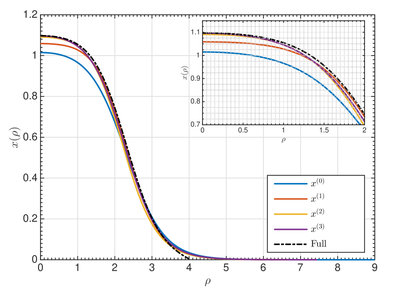
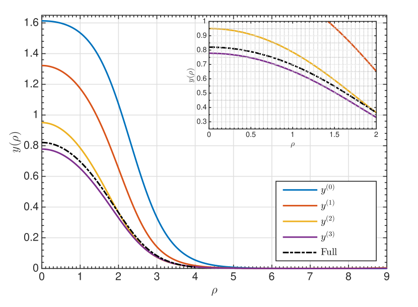
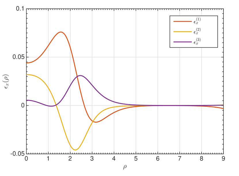
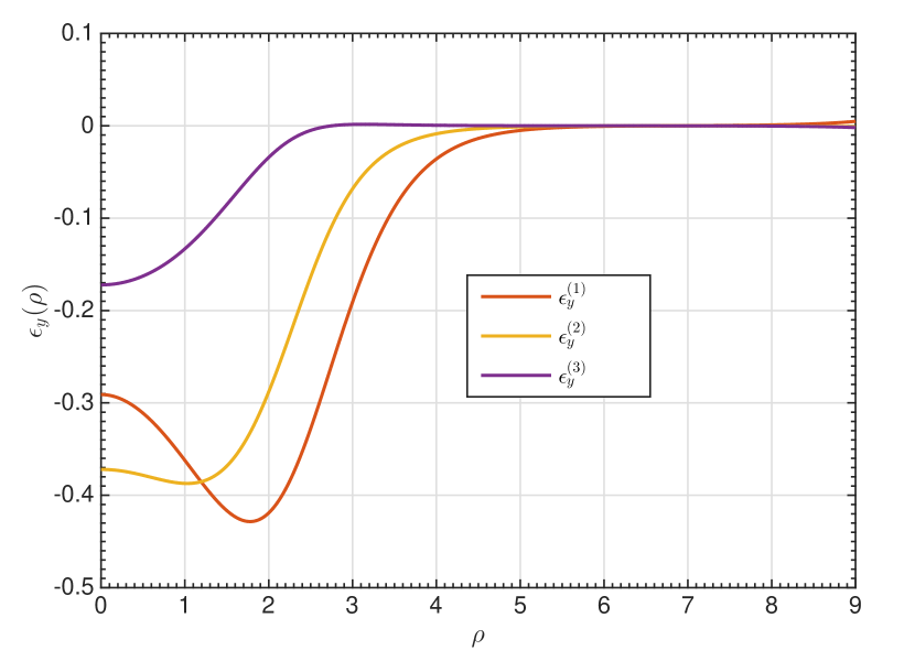
Figure 2: The perturbative algorithm for a two field potential, $V(x,y)$. The top two panels show the field profiles $x(\rho)$ and $y(\rho)$ at each iteration starting from a kink ansatz (solid blue), and converging to the true solution (dotted black). The bottom two panels show the corrections, $\epsilon$, computed at each step by solving Eq. 38. Figure reproduced from [94].

In practice, we terminate the iteration once the iterates satisfy a set of convergence criteria to within a predetermined numerical tolerance. There are several possible convergence criteria. Ref. [94] suggests the vanishing of the inhomogeneous terms, Eq. 39, to within a specified tolerance. These, of course, vanish for the exact bounce solution. By default, we instead specify thresholds for the relative changes in the action, $\kappa_{S}$, and initial values of the fields, $\kappa_{\phi}$, and store the Euclidean action $S^{(j)}$ and starting position of each field $\phi^{(j)}_{i}(0)$ at each iteration. When both of the following conditions are met:

$$\frac{\left|S^{(j)}-S^{(j-1)}\right|}{\max\left(S^{(j)},S^{(j-1)}\right)}<\kappa_{S},$$ (41)

$$\max_{i}\left(\frac{\left|\phi^{(j)}_{i}(0)-\phi^{(j-1)}_{i}(0)\right|}{\max\left(\phi^{(j)}_{i}(0),\phi^{(j-1)}_{i}(0)\right)}\right)<\kappa_{\phi}$$ (42)

the algorithm terminates and returns the Euclidean action and field profiles.

5.3 Multiple shooting method

As described above, at each step of the perturbative algorithm, one needs to compute correction functions $\epsilon_{i}(\rho)$ by solving the boundary value problem (BVP) in Eq. 38 and Eq. 40 for a system of $N$ linear differential equations (once terms that are $O(\epsilon^{2})$ or higher are neglected). This section will outline a straightforward approach to solving these equations that generalizes the shooting method of Section 4 to multiple fields. However, since we are now operating on linear equations, the algorithm converges in a single step. To simplify the notation, in the following we describe the shooting method as applied to determine the corrections $\epsilon_{i}(\rho)$ to the initial ansatz $A_{i}(\rho)$; the equivalent expressions for later stages of the iteration follow by replacing $A_{i}(\rho)\rightarrow\phi_{i}^{(j)}(\rho)$ and $\epsilon_{i}(\rho)\rightarrow\epsilon_{i}^{(j)}(\rho)$.

The boundary conditions fix $\dot{\epsilon}_{i}(0)=-\dot{A}_{i}(0)$. Solving the BVP means finding initial values $\epsilon_{i}(0)\equiv\epsilon_{0i}$ such that integrating from the initial conditions yields a solution satisfying

$$\epsilon_{i}(\rho\to\infty)={\phi_{f}}_{i}-A_{i}(\rho\to\infty).$$ (43)

In fact, we work on a finite domain $[\rho_{\text{min}},\rho_{\text{max}}]$ to avoid problems due to the $n/\rho$ term in Eq. 18. Since we use Eq. 33 to calculate the action, and our boundary conditions require that the derivatives $\dot{\phi}_{i}(\rho)$ vanish as $\rho\rightarrow\infty$ and as $\rho\rightarrow 0$, for sufficiently small $\rho_{\text{min}}$ and large $\rho_{\text{max}}$ the action calculation remains accurate. On the finite domain, the boundary conditions become

$$\epsilon_{i}(\rho_{\text{max}})={\phi_{f}}_{i}-A_{i}(\rho_{\text{max}}),\quad\dot{\epsilon}_{i}(\rho_{\text{min}})=-\dot{A}_{i}(\rho_{\text{min}}).$$ (44)

We want to solve the second order system

$$\ddot{\epsilon}_{i}+\frac{n}{\rho}\dot{\epsilon}_{i}-\left.\sum_{j}\frac{\partial^{2}V(\phi)}{\partial\phi_{i}\partial\phi_{j}}\right|_{A(\rho)}\epsilon_{j}=B_{i}(\rho),$$ (45)

with $B_{i}(\rho)$ as given in Eq. 39. This may be reduced in the usual manner to a system of $2N$ first order equations for $\epsilon_{i}$ and the new variables

$$\zeta_{i}\equiv\dot{\epsilon_{i}},$$ (46)

implying

$$\dot{\zeta}_{i}=B_{i}(\rho)+\left.\sum_{j}\frac{\partial^{2}V(\phi)}{\partial\phi_{i}\partial\phi_{j}}\right|_{A(\rho)}\epsilon_{j}-\frac{n}{\rho}\zeta_{i}.$$ (47)

We solve this system using a form of Newton’s method [104], suitably generalized for more than one field.

It is instructive to write the system in matrix form,

$$\dot{\bm{x}}(\rho)=C(\rho)\,\bm{x}(\rho)+\bm{b}(\rho),$$ (48)

where $\bm{x}(\rho)=(\epsilon_{1},...,\epsilon_{N},\zeta_{1},...,\zeta_{N})^{T}$, $\bm{b}(\rho)=(0,\ldots,0,B_{1}(\rho),\ldots,B_{N}(\rho))^{T}$, and $C(\rho)$ is a $2N\times 2N$ block matrix:

$$C(\rho)=\begin{pmatrix}0&\mathds{1}\\ J&P\end{pmatrix},\ P_{ij}=-\frac{n}{\rho}\delta_{ij},\ J_{ij}=\frac{\partial^{2}V(\phi)}{\partial\phi_{i}\partial\phi_{j}}\Big{|}_{A(\rho)}.$$ (49)

In the above, $\mathds{1}$ is the $N\times N$ identity matrix and $\delta_{ij}$ is the Kronecker delta. The general solution of Eq. 48 is given by the Peano-Baker series [105],

$$\bm{x}(\rho)=S[\rho,\rho_{\text{min}}]\,\bm{x}(\rho_{\text{min}})+\int_{\rho_{\text{min}}}^{\rho}S[\rho,s]\bm{b}(s)ds,$$ (50)

where $S[\rho,\rho^{\prime}]$ is a linear operator for all $\rho>\rho^{\prime}$. The important thing about this representation is that if we write our initial conditions as

$$\bm{x}(\rho_{\text{min}})=\begin{pmatrix}\bm{\epsilon}(\rho_{\text{min}})\\ \bm{\zeta}(\rho_{\text{min}})\end{pmatrix},$$ (51)

and note that the components of $\bm{\zeta}(\rho_{\text{min}})$ are fixed by the second set of boundary conditions in Eq. 44, we can consider integrating the equations from $\rho_{\text{min}}$ to $\rho_{\text{max}}$ as an affine map $\mathcal{E}$ between the initial and final values for $\bm{\epsilon}$ only,

$$\mathcal{E}\left[\bm{\epsilon}(\rho_{\text{min}})\right]\equiv\bm{\epsilon}(\rho_{\text{max}})=\tilde{S}[\rho_{\text{max}},\rho_{\text{min}}]\,\bm{\epsilon}(\rho_{\text{min}})+B[\rho_{\text{min}},\rho_{\text{max}}].$$ (52)

Here $B[\rho_{\text{min}},\rho_{\text{max}}]$ is the first $N$ entries of the inhomogeneous term in Eq. 50, and $\tilde{S}[\rho_{\text{max}},\rho_{\text{min}}]\equiv\pi\circ S[\rho_{\text{max}},\rho_{\text{min}}]$ where $\pi$ denotes projection onto the first $N$ coordinates. We can obtain an estimate for $\tilde{S}[\rho_{\text{max}},\rho_{\text{min}}]$ with $N+1$ integrations. Fixing an initial guess $\bm{\epsilon}^{0}$, we may write

$$\tilde{S}[\rho_{\text{max}},\rho_{\text{min}}]_{ij}=\frac{\partial\mathcal{E}_{i}}{\partial\epsilon_{j}}\approx\frac{\mathcal{E}_{i}(\epsilon^{0}_{1},...\epsilon^{0}_{j}+\Delta\epsilon,...,\epsilon_{N})-\mathcal{E}_{i}(\epsilon^{0}_{1},...,\epsilon_{N})}{\Delta\epsilon}.$$ (53)

To satisfy the boundary condition $\bm{\epsilon}(\rho_{\text{max}})=\bm{\phi_{f}}-\bm{A}(\rho_{\text{max}})\equiv\hat{\bm{\epsilon}}$, we need to find a correction $\delta\bm{\epsilon}$ to our initial guess such that $\mathcal{E}(\bm{\epsilon}^{0}+\delta\bm{\epsilon})=\hat{\bm{\epsilon}}$. Since

$$\mathcal{E}(\bm{\epsilon}^{0}+\delta\bm{\epsilon})-\mathcal{E}(\bm{\epsilon}^{0}) =\tilde{S}[\rho_{\text{max}},\rho_{\text{min}}]\delta\bm{\epsilon}$$ (54)

$$=\hat{\bm{\epsilon}}-\mathcal{E}(\bm{\epsilon}^{0}),$$

$\delta\bm{\epsilon}$ can be obtained by solving the linear system $\tilde{S}[\rho_{\text{max}},\rho_{\text{min}}]\delta\bm{\epsilon}=\hat{\bm{\epsilon}}-\mathcal{E}(\bm{\epsilon}^{0})$. The algorithm to compute the next correction $\bm{x}(\rho)$ is then complete after a final integration from the corrected initial conditions,

$$\bm{x}(\rho_{\text{min}})=\begin{pmatrix}\bm{\epsilon}^{0}+\delta\bm{\epsilon}\\ -\dot{\bm{A}}(\rho_{\text{min}})\end{pmatrix}.$$ (55)

6 BubbleProfiler structure

BubbleProfiler is a C++ software package for finding the bounce solution and outputting the bounce action and field profiles. BubbleProfiler is designed so that multiple methods for finding the bounce solution may be implemented. Currently the main bounce solver is a perturbative algorithm described in Section 5, which uses the multiple shooting method described in Section 5.3 to solve the linearized correction equations. Additionally, a fast implementation of the nonlinear direct shooting method outlined in Section 4 is available to solve single-field problems. We intend BubbleProfiler to become a mature software package suitable for widespread use in scientific research, and integration into larger phenomenology frameworks. Reflecting this ambition, BubbleProfiler includes:

• A comprehensive suite of unit tests.

• Detailed Application Programming Interface (API) documentation.

• A modular architecture designed using the dependency injection principle for maximum flexibility.

• A large selection of example scripts illustrating the use of the code.

• A continuous integration pipeline which automatically builds, tests, and updates the API documentation when changes are made to the code.

Detailed and up to date API documentation, including instructions for the installation and usage of the code are available at https://bubbleprofiler.github.io/.

6.1 BubbleProfiler Architecture

Figure 3 illustrates the perturbative algorithm BubbleProfiler uses to find the bounce action when there is more than one field. In the following we describe each step, providing a brief summary of how they are implemented in the code. BubbleProfiler uses an object-oriented modular design with so-called interface (or abstract) classes in many cases, to allow a given component to have more than one implementation and ensure maximum flexibility and extensibility. For a complete reference to BubbleProfiler, see the API documentation.

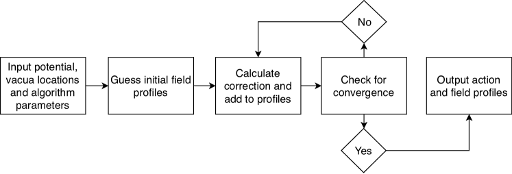
Figure 3: Schematic showing the high level structure and execution flow of BubbleProfiler. A typical execution begins with the user providing a potential, the locations of the true and false vacua, and configuration parameters for the algorithm. These are used to construct an initial profile guess (ansatz). The main execution loop then consists of computing corrections to the ansatz using multiple shooting, adding the correction to the ansatz, and checking for convergence. Once the specified convergence criteria are met, the code outputs the resulting field profiles and Euclidean action.

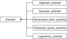
Figure 4: Potential class hierarchy.

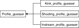
Figure 5: Profile guesser class hierarchy.

Input potential

An essential input for any bounce solver is the potential for which the bounce action must be solved. BubbleProfiler contains an interface class Potential for representing real valued functions of one or more scalar fields with methods for evaluating partial derivatives and making linear changes of coordinates that must be given in the inherited class. Specific implementations for the potential are then derived from this as shown in Fig. 4. The Algebraic_potential class is currently used in BubbleProfiler by default. It uses GiNaC’s [106] symbolic manipulation capabilities so that users can input arbitrary algebraic expressions as potentials without writing any code. This also has the advantage that derivatives and changes of coordinates can be implemented at the algebraic level, which improves overall performance. This is because in general, pre-computing algebraic derivatives will be faster than using finite difference methods on each evaluation. An additional set of derived classes are provided for testing purposes. These are Gaussian_potential, Generalized_fubini_potential, Logarithmic_potential, Restricted_quartic_potential, and Thin_wall_potential. Full descriptions of these potentials may be found in the API documentation. Users who require potentials that cannot be expressed via Algebraic_potential are encouraged to implement their own subclasses of Potential. Details of the Potential interface may be found in the API documentation. We encourage users to contact the authors with any questions about subclassing Potential.

Input vacua locations

The purpose of the bounce action solver is to find the bounce action for phase transitions between two vacua. Therefore a necessary starting point is the location of these minima. The user may specify the locations of both the true and false vacua in field coordinates. If the false vacuum location is not supplied, the code assumes it is located at the origin. If the true vacuum is not supplied, the code will attempt to locate a global minimum using the NLopt optimization library [107].

Algorithm parameters

A number of options that control the execution of the algorithm may be specified. If using the command line interface, these are configured using the options specified in Appendix C. If using the code directly, the primary configuration points are the Generic_perturbative_profiler class and the associated Profile_convergence_tester using the setter methods described in the API documentation. Available parameters include:

• The domain boundaries, $\rho_{\text{min}}$ and $\rho_{\text{max}}$. If these are not specified, the code will attempt to determine appropriate values based on the initial ansatz. The domain start is estimated by finding the point closest to the origin where the radial derivative of the ansatz field profile is equal to $10^{-5}$, while the domain end is chosen to be the outermost point at which the ansatz field profile is less than or equal to $10^{-5}$.

• The integration algorithm. Currently, Runge-Kutta (RK4) and the Euler method are supported.

• Discretization parameters for integration and interpolation, namely the step-size and the fraction of those points that are used in spline representations.

• Tolerances for testing whether the algorithm has converged. These can be specified in terms of the Euclidean action, the field values at $\rho_{\text{min}}$, or both.

• Maximum number of iterations. If the convergence tests do not pass before this threshold, an error is issued.

• Whether to use the perturbative algorithm or the direct shooting method for single field problems.

Guess initial field profiles

In the first step of the BubbleProfiler algorithm the above inputs – potential, vacua locations, and algorithm parameters – are used to construct an initial set of field profiles representing an ansatz solution to the bounce equations in Eq. 18. To ensure flexibility and extensibility, we allow multiple options for constructing the ansatz by defining an abstract base class Profile_guesser. The different types of ansatz are implemented as derived subclasses, as shown in Figure 5. The two main subclasses are Kink_profile_guesser, which uses the parametric ansatz form given by Eq. 36, and Shooting_profile_guesser which applies the direct shooting method of Section 4 to the reduced one-dimensional potential connecting the vacua. Kink_profile_guesser is the default and is slightly faster as it does not involve numerical integration. Shooting_profile_guesser may be of use in unusual cases where the kink ansatz does not describe a good initial bubble profile. In either case, the resulting set of field profiles is an object from the Field_profiles class, which uses the eigen3 fast linear algebra library [108] to store a (number of fields) $\times$ (number of grid points) discrete representation of the bubble profile. As this array only stores a finite number of points, the class also uses the GSL library [109] to build cubic spline interpolants. This allows off-grid evaluation and fast calculation of derivatives using algebraic rather than finite difference methods. Finally, Instream_profile_guesser allows the user to provide a text file or other input stream containing an ansatz solution. This was developed for testing purposes, but may be of use for difficult potentials if there are convergence problems with the standard ansatz methods. Users may also implement their own subclasses of Profile_guesser for problems where the provided ansatz types are not sufficiently close to the true solution .

Calculate corrections and add perturbative correction

An iteration is then performed to perturbatively find the bounce action and field profile. At each step in the iteration a perturbative correction is calculated, and used to update the field profile. Given a set of field profiles containing an ansatz or partial solution, BubbleProfiler computes a correction function $\bm{\epsilon}$ by solving the linearized perturbation Eq.s 38. The Generic_perturbative_profiler class accomplishes this via multiple shooting method detailed in Section 5.3. Note that as implemented, this class is the main entry point for the code, and orchestrates the iterative process of successively correcting the profiles until the convergence criteria are met. It is generic in the sense that the user must provide implementations of key dependencies such as the convergence tester, ODE integration algorithm, and profile guesser. This dependency injection design strategy is intended to facilitate flexibility and interchangeability of components.

Convergence check

After each perturbative correction to the field profiles, a check is performed to determine if the algorithm has converged. This check is implemented in the Relative_convergence_tester class. Objects from this class are stateful and keep track of the Euclidean action $S$ and starting field values $\phi_{i}(0)$ at each iteration. Once the relative changes (defined in Eq. 41 and Eq. 42) fall below the corresponding thresholds rtol_action and rtol_fields, the algorithm terminates.

Output

Once the algorithm has converged, the Generic_perturbative_profiler stores the completed Field_profiles and Euclidean action, and makes these available via method calls get_bubble_profile and get_euclidean_action.

The direct shooting method that can be used for single field problems has the same inputs and outputs as shown in Figure 3, though the specific Algorithm parameters that are used differ, see Appendix C.3 for options specific to the single-field case. However the iteration shown in Figure 3, which connects the inputs and outputs, is replaced with the shooting method described in Section 4. This is mostly self-contained in the Shooting class and sufficient details about the code for this have already been given in Section 4, therefore we omit further details on this here.

7 Comparisons with existing codes and analytic solutions

In this section we compare the robustness and performance of our new code, BubbleProfiler, comparing to analytic results and against existing approaches, CosmoTransitions, written in python and AnyBubble, written in Mathematica. Before presenting the comparisons we will briefly describe the methods CosmoTransitions and AnyBubble use to find the bounce solution. To test the accuracy and correctness we will look at the action calculated by BubbleProfiler for a special set of potentials where there are known analytic solutions. We will then look at a more general 1-d potential where there is no analytic solution and compare BubbleProfiler to CosmoTransitions, and investigate the performance of these codes. Finally we will compare BubbleProfiler to AnyBubble for multi-field potentials with those of CosmoTransitions and AnyBubble. All tests were executed on a desktop system running Ubuntu 16.04, equipped with an Intel i7-4790 3.60 GHz processor and 16 GB of DDR3 RAM clocked at 1.6 GHz.

7.1 CosmoTransitions and AnyBubble

For one-field cases CosmoTransitions implements a shooting method in Python, which is similar to the direct shooting method implemented in BubbleProfiler. For potentials with more than one field CosmoTransitions [78] uses a so-called path-deformation algorithm. The path $\vec{\phi}(\rho)$ is rewritten in intrinsic coordinates, parameterized by the distance along the path, $x$. The equation of motion separates into two pieces

$$\ddot{x}+\frac{n}{\rho}\dot{x} =\frac{\partial V[\vec{\phi}(x)]}{\partial x},$$ (56)

$$\frac{d^{2}\vec{\phi}}{dx^{2}}\,\dot{x}^{2} =\vec{\nabla}_{\perp}V(\vec{\phi}).$$ (57)

The first equation describes the motion along the path whereas the second describes normal forces along the path. For a solution, the normal force,

$$\vec{N}\equiv\frac{d^{2}\vec{\phi}}{dx^{2}}\,\dot{x}^{2}-\vec{\nabla}_{\perp}V(\vec{\phi}),$$ (58)

must vanish such that the second equation is satisfied. In the path-deformation algorithm, the motion along the trajectory, $x(\rho)$, is solved with a shooting method, and the path $\vec{\phi}(\rho)$ is perturbed by $\Delta\vec{\phi}(\rho)\propto\vec{N}(\rho)$. This process is iterated until:

$$\frac{\vec{N}_{max}}{|\nabla V|_{max}}<\kappa,$$ (59)

where $N_{max}$ and $|\nabla V|_{max}$ are respectively the largest values of the normal force (equation 58) and potential gradient along the bounce path, and $\kappa$ is a configurable parameter .

AnyBubble [80], on the other hand, uses a multiple shooting method. The time domain is divided into $n$ subdomains, with boundaries at $\rho_{0},\,\rho_{1},\,\ldots\text{ and }\rho_{n}$. The states at the beginning of each subdomain, that is $\phi(\rho_{i})$ and $\dot{\phi}(\rho_{i})$, are unknown, but must match the final states of the previous subdomains. They are matched using Powell’s hybrid method. By stitching together solutions in each subdomain, the method finds a solution for the whole domain.

7.2 Thin-wall

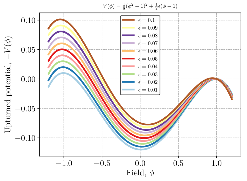
(a) Potential

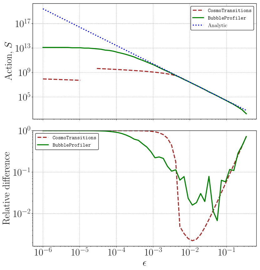
(b) Action

Figure 6: (6(a)) Thin-wall potential in Eq. 60. (6(b)) Euclidean action in $d=4$ for small values of $\epsilon$. The top panel compares the analytic solution to BubbleProfiler and CosmoTransitions. The bottom panel shows the relative difference between each code and the analytic solution. In the region where the bounce solutions from both codes agree well with the thin wall approximation, BubbleProfiler is generally more accurate than CosmoTransitions. However, in the limit of small $\epsilon$ the action diverges and both codes fail to match the analytic formula.

As discussed in Section 4, when the true and false vacua of a single-field potential are nearly degenerate, the bounce solution describes a thin-walled bubble. This poses numerical difficulties for the direct shooting method, as the system becomes extremely sensitive to initial conditions. Fortunately, the reparameterization Eq. 30 solves this problem in BubbleProfiler and CosmoTransitions also makes use of this trick. Therefore in this section we investigate how well these codes reproduce a known thin-wall solution [1].

For $\epsilon/(a^{2}\lambda)\ll 1$, the potential,

$$V(\phi)=\frac{\lambda}{8}(\phi^{2}-a^{2})^{2}+\frac{\epsilon}{2a}(\phi-a),$$ (60)

has extrema at $\phi_{t}\approx-a$, $\phi_{b}\approx\epsilon/(a^{3}\lambda)$ and $\phi_{f}\approx a$. The thin-wall solution [1] is,

$$S=\frac{8\pi^{2}a^{12}\lambda^{2}}{3\epsilon^{3}}.$$ (61)

for $n=3$ and

$$S=\frac{128\pi a^{9}\lambda^{3/2}}{81\epsilon^{2}}$$ (62)

for $n=2$, where $n$ appears in Eq. 5 and can be related to the number of space-time dimensions, $d$, of the action which is being calculated, through $n=d-1$.

We checked our code for this potential for $d=4$ in examples/thin-wall/thin_wall.cpp, which is built by make thin and executed by bin/thin.x <lambda> <a> <epsilon>. In Fig. 6(a) we show the how the shape of the potential, for fixed $\lambda=a=1$, changes as $\epsilon$ is varied in discrete steps between 0.1 and 0.01, illustrating how the the thin walled limit is approached as $\epsilon\rightarrow 0$. Fig. 6(b) then compares the analytic solution to BubbleProfiler and CosmoTransitions, varying $\epsilon$ in the range $(10^{-6},10^{-0.35})$, again fixing $\lambda=a=1$. Reading Fig. 6(b) from right to left one can see that initially we are away from the thin-walled limit, but as $\epsilon$ is decreased BubbleProfiler and CosmoTransitions approach the thin-walled, limit reproducing the analytic solution to within $10^{-1}$ or $10^{-2}$ respectively. However as $\epsilon$ is reduced further BubbleProfiler and CosmoTransitions begin to again diverge from the thin-walled limit, showing that sufficiently thin-walled cases are still problematic as one would would expect.

7.3 Fubini potential

There is also a known analytic result for the generalized Fubini potential,

$$V(\phi)=\frac{4um^{2}(m-1)}{2m+1}\phi^{(2m+1)/m}-2uvm^{2}\phi^{(2m+2)/m},$$ (63)

which results in the bounce action [110]

$$S=\frac{m\pi^{2}}{(4m^{2}-1)}\frac{1}{uv^{2m-1}},$$ (64)

for $n=3$. We checked our code for this potential in examples/general-fubini/general_fubini.cpp, which is built by make fubini and bin/fubini.x <u> <v> <m>. We compared the analytic solution to BubbleProfiler and CosmoTransitions using $u=v=1$, and varying $m=1+\Delta m$ in the range $\Delta m=(10^{-4},10^{2})$. The results are summarized in Figure 7, where we again illustrate how the shape of the potential changes on the left hand side. On the right hand side we present results for the action for BubbleProfiler, CosmoTransitions and the analytic solution in the top panel and in the bottom panel show the relative difference between the analytic solution and the action calculated by the two codes. For $\Delta m<10^{-1}$, the accuracy of the two codes is comparable, though both codes struggle with precise agreement with the analytic solution. This is because as $\Delta m\to 0$ the barrier vanishes resulting in an infinitely thick-wall and consequently numerical problems. For $\Delta m>1$, CosmoTransitions fails to produce a solution, while BubbleProfiler matches the analytic solution to within a tolerance of $10^{-1}$.

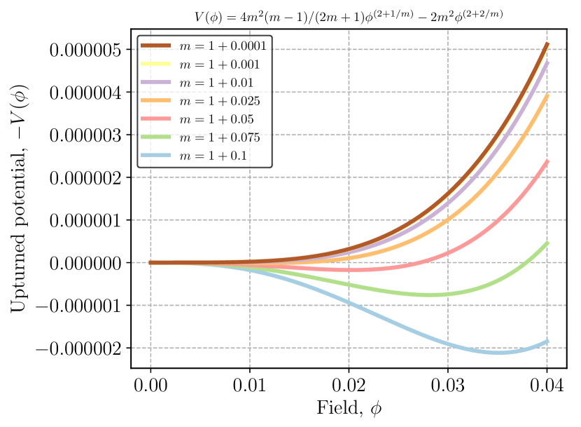
(a) Potential

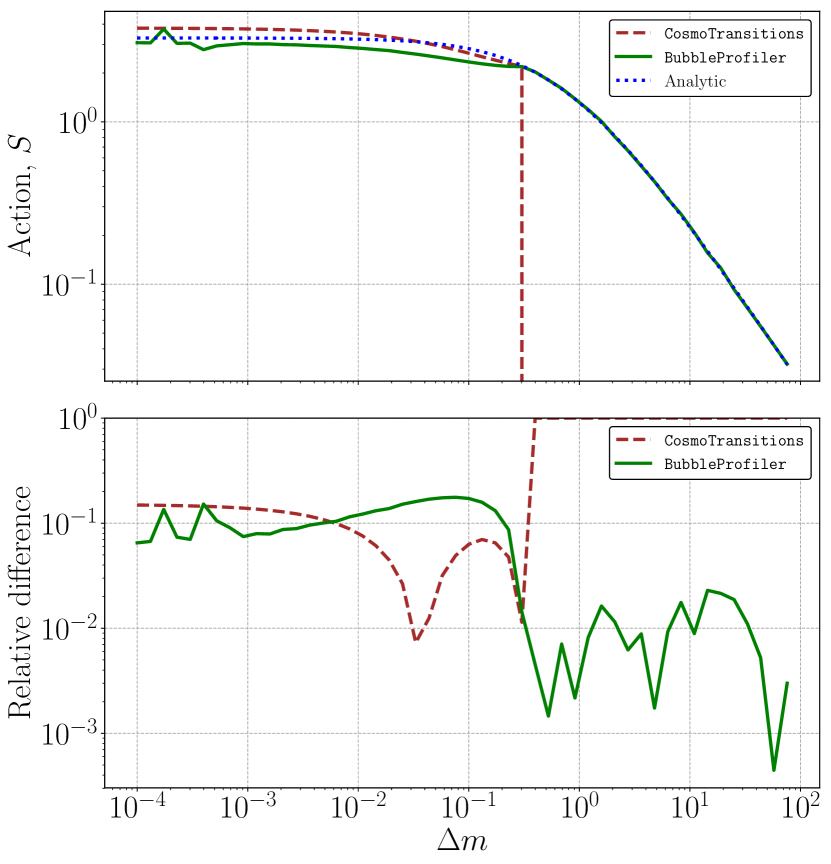
(b) Action

Figure 7: (7(a)) Fubini potential in Eq. 63. (7(b)) Euclidean action of the analytic solution, BubbleProfiler, and CosmoTransitions with absolute values (top) and relative difference (bottom).

7.4 Logarithmic potential

Another potential with known analytic solutions is the logarithmic potential,

$$V(\phi)=\frac{1}{2}m^{2}\phi^{2}\left[1-\ln\left(\frac{\phi^{2}}{w^{2}}\right)\right],$$ (65)

and this results in the bounce action [110]

$$S=\frac{\pi^{2}e^{4}}{2}\frac{w^{2}}{m^{2}},$$ (66)

for $n=3$. We checked our code for this potential in examples/logarithmic/logarithmic.cpp, which is built by make logarithmic and executed by bin/logarithmic.x <m> <w>. We compared the analytic solution to BubbleProfiler and CosmoTransitions using $m=1$ and varying $\omega$ in the range $(10^{-4},10^{1})$. The results are summarized in Figure 8. We found that for this potential, CosmoTransitions was more accurate with the difference being most pronounced for low values of $\omega$.

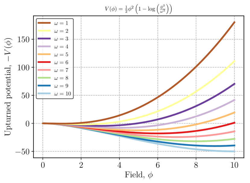
(a) Potential

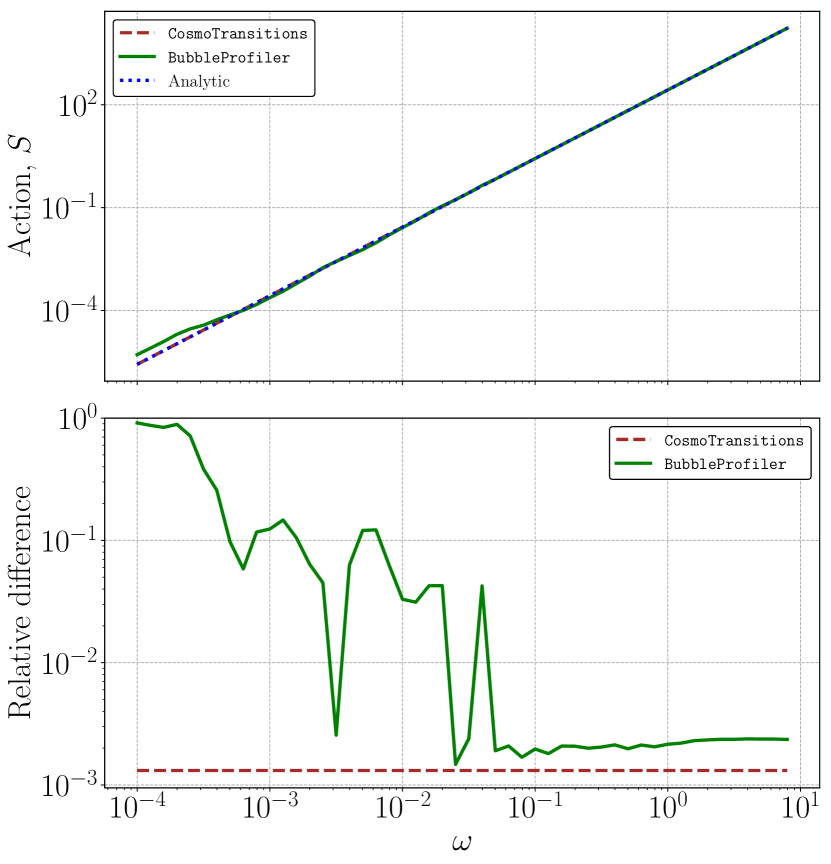
(b) Action

Figure 8: (8(a)) Logarithmic potential in Eq. 65. (8(b)) Euclidean action of the analytic solution, BubbleProfiler, and CosmoTransitions with absolute values (top) and relative difference (bottom).

7.5 Renormalizable single-field potentials

We now consider potentials of the form

$$V(\phi)=\frac{-4\alpha+3}{2}\phi^{2}-\phi^{3}+\alpha\phi^{4}.$$ (67)

Solutions to arbitrary order-four polynomials are related by rescalings to solutions to this restricted order-four polynomial, as we will now describe.

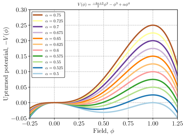
Figure 9: Quartic potential in Eq. 67 for $\alpha=(0.5,0.75)$. The parameter $\alpha$ smoothly interpolates between thin and thick-walled potentials. For $\alpha\simeq 0.5$, the true vacuum, $\phi_{t}=1$, and the false vacuum, $\phi_{f}=0$, are degenerate and the bounce is thin-walled, whereas for $\alpha\simeq 0.75$, the barrier and the false minimum nearly coincide and the solution is thick-walled.

Any potential with two minima separated by a local maxima can be approximated by a quartic potential, which naively has five free parameters. However, four of these parameters are redundant as bounce solutions to classes of potentials related by trivial transformations are themselves related by trivial transformations. Specifically, the bounce action is invariant under the transformations $\phi\to\phi+\Delta\phi$ and $V\to V+\Delta V$, eliminating two parameters. The transformation $V\to V/a$ changes the action by $S\to\sqrt{a}S$ for $d=3$ and by $S\to aS$ for $d=4$, and eliminates a further parameter. Finally, we may work in units of our choice: the changes of unit, $\phi\to\phi/b$ etc, result in $S\to S/b$ for $d=3$, and leave the action unchanged in $d=4$ as it is dimensionless.

This leaves a single parameter relevant for solving the bounce equation and thus we may make the problem a single parameter problem. Beginning with a general renormalizable potential,

$$V(\phi)=\Lambda^{4}+t\phi+m^{2}\phi^{2}+\kappa\phi^{3}+\lambda\phi^{4},$$ (68)

with true vacuum $\phi_{t}$ and false vacuum $\phi_{f}$, we shift the potential such that the false vacuum is at the origin and pick units such that the true vacuum is at $\phi=1$. We rescale the potential such that the coefficient of the cubic term is minus one and remove the constant piece. We are left with a potential described by a single parameter $\alpha$,

$$V(\chi)=\frac{-4\alpha+3}{2}\chi^{2}-\chi^{3}+\alpha\chi^{4},$$ (69)

where

$$\alpha=\lambda\left|\frac{\phi_{t}-\phi_{f}}{\kappa+4\lambda\phi_{f}}\right|.$$ (70)

By the fact that the true vacuum is at $\chi=1$ and thus $V(\chi=1)<V(\chi=0)$, and the fact that the origin is a minima, $V^{\prime\prime}(\chi=0)>0$, we require $1/2<\alpha<3/4$ for consistency. In Figure 9 we plot potentials with $\alpha$ varying over this range in steps of $0.025$.

We denote the action for this potential by $S(\alpha)$. The action for the original, general quartic potential depends on a potential-specific factor that simply scales $S(\alpha)$. For $d=3$,

$$S=|\phi_{t}-\phi_{f}|\sqrt{\frac{\lambda}{\alpha}}\,S(\alpha).$$ (71)

and for $d=4$,

$$S=\frac{\lambda}{\alpha}\,S(\alpha).$$ (72)

Thus it suffices to consider $S(\alpha)$ and potentials parameterized by $\alpha$. We find from a thin-wall approximation assuming $\alpha\simeq 1/2$ that for $d=3$,

$$S(\alpha)=\frac{2\pi}{81}\frac{1}{(\alpha-1/2)^{2}},$$ (73)

and for $d=4$,

$$S(\alpha)=\frac{\pi^{2}}{96}\frac{1}{(\alpha-1/2)^{3}}.$$ (74)

We checked our code for this potential in examples/quartic/action.cpp, which is built by make quartic and executed by bin/quartic.x <E> <alpha> <dim>. The result may be tabulated for $E=1$ by the program examples/quartic/tabulate.cpp, which is built by make quartic_tabulate and executed by
bin/quartic_tabulate.x <dim> <min-alpha> <max-alpha> <step>. The perturbative algorithm is intended for multi-field cases, but we also include it in this analysis for purposes of comparison.

As discussed in Section 7.2 there is a known analytic solution in the thin-walled limit. With the parameterization Eq. 69, $\alpha$ controls the degree of degeneracy. In particular, as $\alpha\rightarrow 0.5$, the vacua become degenerate and the bounce solution approaches a step function [94].

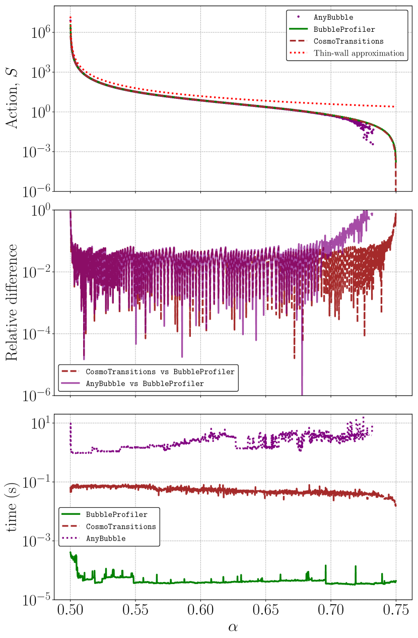
(a) Shooting method

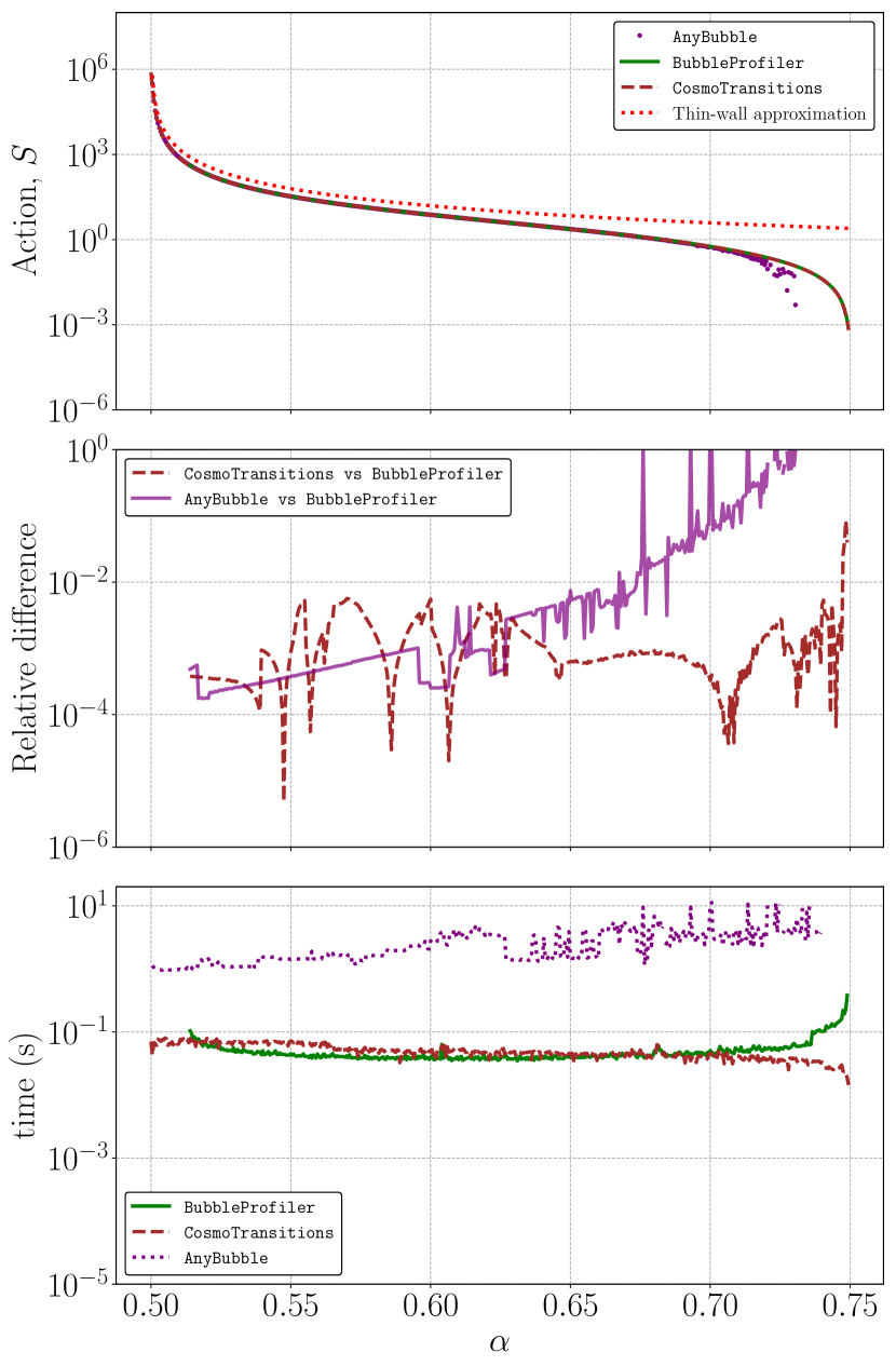
(b) Perturbative algorithm

Figure 10: Comparison of (10(a)) direct shooting with BubbleProfiler and direct shooting with CosmoTransitions and AnyBubble, and (10(b)) the perturbative algorithm implemented by BubbleProfiler with initial-step-size set to 0.1 and direct shooting with CosmoTransitions and AnyBubble. The potential is given by Eq. 68, with $E=1$ and $\alpha\in(0.5,0.75)$. From top to bottom, the three panels in each chart show the Euclidean action, $S_{E}$; the relative difference in $S_{E}$ between BubbleProfiler and CosmoTransitions and between BubbleProfiler and AnyBubble; and the execution time.

Figure 10 shows that when using the direct shooting method, BubbleProfiler outperforms CosmoTransitions, and — excepting the asymptotic cases $\alpha\rightarrow 0.5$ and $\alpha\rightarrow 0.75$ — computes the same Euclidean action to within a factor of $10^{-1}$. Since the direct shooting part of BubbleProfiler is a C++ implementation of the algorithm in CosmoTransitions (a Python code), this is unsurprising. For single field problems, the speed of the perturbative algorithm depends strongly on the initial-step-size setting. With initial-step-size set to 0.1, which we used here and in testing delivered a stable action calculation without degradation of the precision, we find timings that are quite similar to that of CosmoTransitions for all $\alpha$ other than those close to the asymptotic limits. In fact in this range the agreement between the perturbative method of BubbleProfiler and CosmoTransitions is actually slightly higher, with the two codes agreeing within $10^{-2}$. However the perturbative method fails consistently for thin walled cases with $\alpha<0.51$. This thin-walled problem will be discussed further when we consider multi-field potentials. For thick walls there is also some performance degradation and agreement between the codes is a little worse.

7.6 Multi-field potentials

7.6.1 Thin walled bubbles in multi-field potentials

In applying the perturbative algorithm to single field potentials we found that cases with near-degenerate vacua resulting in thin walled bubbles became problematic for $\alpha<0.51$. To investigate whether this problem generalized to multi-field potentials we implemented the Gaussian_Potential class. This class implements a potential of the form:

$$V(\phi)=-(N(\phi,0)+\gamma N(\phi,\mu)),$$ (75)

where

$$N(\phi,\mu)=\frac{1}{(2\pi)^{n/2}}\text{exp}\bigg{(}-\frac{1}{2}|\phi-\mu|^{2}\bigg{)}$$ (76)

is a unit n-dimensional Gaussian, $\gamma$ controls the relative depth of the minima, and $\mu=1/\sqrt{n}(\lambda,...,\lambda)$ so that $\lambda$ is the geometric distance between minima. As $\gamma\rightarrow 1$, the vacua approach degeneracy and the solution becomes thin walled. We tested potentials of up to five fields and found that the problem generalized in a straightforward way - if the value of $\alpha$ corresponding to the single-field potential used to fit the ansatz approached $0.51$, the profiler failed to converge.

In light of this result, we added a check which compares the ansatz $\alpha$ to a threshold Kink_profile_guesser::alpha_threshold = 0.514. An error is issued if the value is less than the threshold. Note that this check is only applied when using the perturbative algorithm. For single field potentials, the shooting method can be used to solve thin walled bounces.

7.6.2 Multi-field potentials — comparison with other codes

For $n>1$ fields, the direct shooting method of Section 4 is no longer applicable. We devised a set of non-physical, polynomial potentials of between one and eight fields for the purposes of comparison. To compare the performance of all three algorithms, and the extent to which they agree on the Euclidean action of the bounce solution, each code was run on these test potentials; the results are summarized in Table 1. The potentials used are listed in Appendix B. These tests are also included as a script in the bubbler tool (see Appendix A) called n_fields_from_interface.py

The BubbleProfiler test results were obtained by executing commands of the form:

⬇

run_cmd_line_potential.x --force-output --write-profiles --potential <potential> --field <fields> --initial-step-size=0.1 --domain-start -1.0 --domain-end -1.0 --local-minimum 0.0 --local-minimum 0.0 --global-minimum 1.0 --global-minimum 1.0 --rtol-action 0.001 --rtol-fields 0.001 --integration-method runge-kutta-4

substituting appropriate values of <potential> and <fields> for each test.

	Action			Time (s)
# fields	BP	CT	AB	BP	CT	AB
1	54.1	52.6	52.4	0.051	0.066	1.285
2	20.8	21.1	20.8	0.479	0.352	7.473
3	22.0	22.0	22.0	0.964	0.215	25.209
4	55.9	56.4	55.9	1.378	0.255	54.258
5	16.3	16.3	16.3	2.958	0.367	305.531
6	24.5	24.5	24.4	4.853	0.337	830.449
7	36.7	36.6	36.7	6.754	0.375	1430.892
8	46.0	46.0	46.0	10.014	0.409	1805.713

Table 1: Test results for potentials of $1$–$8$ fields for BubbleProfiler (BP), CosmoTransitions (CT), and AnyBubble (AB). BubbleProfiler was configured with initial-step-size set to $0.1$ and a stopping criteria of rtol_action = rtol_fields = 0.001 (see Section 5.2). The comparable parameter for CosmoTransitions is fRatioConv (see Eq. 59), which we set to the default value of 0.02. AnyBubble does not have a configurable stopping criterion.

We find that CosmoTransitions is faster than BubbleProfiler for all cases other than the single field case, where BubbleProfiler is slightly faster, though the differences in speed are much less significant when there are only a few fields. AnyBubble is significantly slower than the other two codes, although this may be a reflection of the current Mathematica implementation, rather than the underlying algorithm. The degree to which the codes agree on the Euclidean action varies, but is within $4\%$ in all cases. If we exclude the single field case, where BubbleProfiler uses direct shooting rather than the perturbative algorithm, the codes agree to within $2\%$.

8 Scalar Singlet Model

For a realistic application of BubbleProfiler we now consider a standard model extension where the Higgs sector has an additional (real) scalar singlet field. This scalar singlet model (SSM) is arguably the simplest possible extension of the standard model of particle physics. Nonetheless, despite the minimality of the SSM, it has generated extensive interest as unlike the SM, it can both explain the relic density of dark matter [113, 114] and, relevant for our work here, supports a first order EWPT with the Higgs mass at $125\,\text{GeV}$ [115, 116, 117]. As such this provides a relevant and interesting model for us to illustrate how one can use BubbleProfiler when investigating the properties of the EWPT in a realistic model.

The most general renormalizable potential coupling the Higgs scalar $h$ to the new scalar singlet $s$ depends on eight operators. We, however, impose a $\mathbb{Z}_{2}$ symmetry $s\rightarrow-s$, which permits only five operators in the potential,

$$V_{\text{Tree}}=-\frac{1}{2}\mu_{h}^{2}h^{2}+\frac{1}{4}\lambda_{h}h^{4}+\frac{1}{2}\mu_{s}^{2}s^{2}+\frac{1}{4}\lambda_{s}s^{4}+\frac{1}{4}\lambda_{m}s^{2}h^{2}.$$ (77)

Following Ref. [118] we add only the leading order terms obtained from a high temperature expansion of the one-loop thermal corrections to the potential, which is sufficient for the scenarios we consider. This gives,

$$V_{T}=V_{\text{Tree}}+\frac{1}{2}(c_{h}h^{2}+c_{s}s^{2})T^{2}.$$ (78)

where $c_{h}$ and $c_{s}$ are defined by

$$c_{h} =\frac{1}{48}(9g^{2}+3g^{\prime 2}+2(6h_{t}+12\lambda_{h}+\lambda_{m})),$$ (79)

$$c_{s} =\frac{1}{12}(2\lambda_{m}+3\lambda_{s}),$$ (80)

and $g$, $g^{\prime}$ are the weak charge and weak hypercharge couplings respectively, while $h_{t}$ is the top quark Yukawa coupling.

At high temperatures the terms from the finite temperature potential ensure the quadratic terms have positive coefficients and electroweak symmetry is restored with a global minimum at the origin. We will focus on scenarios where as the temperature cools down a deeper minimum develops in the $h=0$ directions with a non-zero value for singlet field, $\langle s\rangle=w$, which spontaneously breaks the $\mathbb{Z}_{2}$ symmetry. As the temperature cools further the electroweak minima with $\langle h\rangle=v$ and $\langle s\rangle=0$ develops and there is a first order phase transition from the $\mathbb{Z}_{2}$ breaking minimum to the electroweak minimum where the $\mathbb{Z}_{2}$ symmetry is restored. Our aim is to calculate the bounce action for this transition, and we will use this to determine if bubble nucleation takes place and if so, what the nucleation temperature is.

First we require that at zero temperature there is an electroweak symmetry breaking (EWSB) minimum with a vacuum expectation value of $v_{\text{EW}}=246.22$ GeV. This allows us to use the EWSB condition, to fix

$$\mu_{h}^{2}=\lambda v_{\text{EW}},$$ (81)

where this matches the familiar SM relation, since the singlet VEV is zero in the EWSB minimum. Secondly we use the measured value of the Higgs mass, $M_{H}=125.1$ GeV [119] to fix the quartic Higgs coupling,

$$\lambda_{h}=\frac{M_{H}^{2}}{2v^{2}_{EW}}.$$ (82)

Next we require that at the critical temperature $T=T_{C}$ the electroweak vacuum is degenerate with the $\mathbb{Z}_{2}$ breaking minimum. This will allow us to replace one of the remaining parameters with the critical temperature. To do this we again follow Ref. [118], and introduce temperature dependent quadratic couplings, so that the temperature dependence of the potential is absorbed into these couplings,

$$\tilde{\mu}_{h}^{2}(T)=\mu_{h}^{2}-c_{h}T^{2},\ \tilde{\mu}_{s}^{2}(T)=\mu_{s}^{2}+c_{s}T^{2},$$ (83)

and

$$V_{T}=-\frac{1}{2}\tilde{\mu}_{h}^{2}(T)h^{2}+\frac{1}{2}\tilde{\mu}_{s}^{2}(T)s^{2}+\frac{1}{4}\lambda_{h}h^{4}+\frac{1}{4}\lambda_{s}s^{4}+\frac{1}{4}\lambda_{m}s^{2}h^{2}.$$ (84)

We can now investigate the minima at finite temperature. Taking the first derivative with respect to the $h$ field, and evaluating at the symmetry breaking vacuum, where it vanishes, leads to,

$$v^{2}(T)=\frac{\tilde{\mu}_{h}^{2}(T)}{\lambda_{h}}=v^{2}_{\text{EW}}-\frac{c_{h}}{\lambda_{h}}T^{2}.$$ (85)

We obtain a singlet mass at finite temperature through,

$$m_{s}^{2}(T)=\frac{\partial^{2}V_{T}}{\partial s^{2}}\bigg{|}_{\begin{subarray}{c}h=v\\ s=0\end{subarray}}=\tilde{\mu}_{s}^{2}(T)+\frac{1}{2}\lambda_{m}v^{2}(T)$$ (86)

Ref. [118] shows that imposing degeneracy of the symmetric and symmetry breaking vacua at $T=T_{C}$ results in the constraint:

$$m_{s}^{2}(T_{C})=\frac{v^{2}(T_{C})}{2}(\lambda_{m}-2\sqrt{\lambda_{h}\lambda_{s}}).$$ (87)

Inserting this into Eq. 86 and rearranging gives,

$$\tilde{\mu}_{s}^{2}(T_{C})=\mu_{s}^{2}+c_{s}T_{C}^{2}=-v^{2}(T_{C})\sqrt{\lambda_{h}\lambda_{s}},$$ (88)

and noting that from Eq. 85, $v^{2}(T_{C})=v^{2}_{\text{EW}}-\frac{c_{h}}{\lambda_{h}}T_{C}^{2}$, we have:

$$\mu_{s}^{2}=-(v^{2}_{\text{EW}}-\frac{c_{h}}{\lambda_{h}}T_{C}^{2})\sqrt{\lambda_{h}\lambda_{s}}-c_{s}T_{C}^{2}$$ (89)

Since $c_{s},\ c_{h}$ and $\lambda_{h}$ are expressed (cf. Eq.s 79,80 and 82) in terms of $\lambda_{m}$, $\lambda_{s}$ and experimentally measured values, the region of the SSM under study is spanned by parameters $\{\lambda_{s},\lambda_{m},T_{C}\}$.

We constructed a benchmark point with a strong first-order phase transition from a tree-level barrier, $\{T_{C},\lambda_{m},\lambda_{s}\}=\{110\,\text{GeV},1.5,0.65\}$. To find the nucleation temperature we use,

$$\frac{S_{E}(T_{N})}{T_{N}}\approx 140,$$ (90)

where $S_{E}(T)$ is the Euclidean action defined in Eq. 8. Varying the temperature and using BubbleProfiler to evaluate the action, we found that this was reached at $T_{N}\approx 85$ GeV.

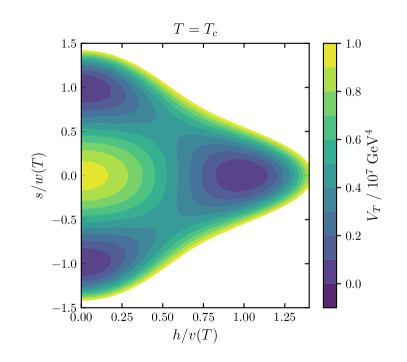
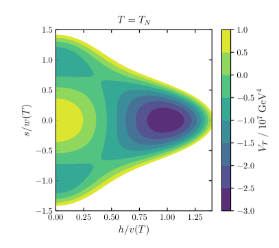
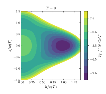
Figure 11: Contour plots of the effective potential for our benchmark SSM point, $\{T_{c},\lambda_{m},\lambda_{s}\}=\{110\ \textrm{GeV},1.5,0.65\}$, at the critical temperature $T=T_{c}$ (top left frame), at the nucleation temperature $T=T_{N}$ (top right frame) and at zero temperature $T=0$ (bottom frame).

Figure 11 shows the structure of the benchmark potential at $T=0$, $T=T_{N}$, and $T=T_{C}$. As described earlier we are considering scenarios where there is a phase transition between a minimum with non-zero $\langle s\rangle=w$ to the electroweak symmetry breaking minimum with $\langle h\rangle=v$ and $\langle s\rangle=0$. In the top left frame of Figure 11 we can see that the electroweak minimum and the $\mathbb{Z}_{2}$ breaking minima are indeed degenerate at $T=T_{c}$, which we have ensured by construction. Note that in this plot the origin has already been destabilized, and is a local maximum. As the temperature cools the electroweak minimum becomes deeper and we reach the nucleation temperature we have calculated using BubbleProfiler and Eq. 90, where the potential has the shape shown by the color contour in the top right frame of Figure 11. After the phase transition the temperature continues to cool down and at $T=0$ the potential has the shape shown in the bottom frame of Figure 11 with an EWSB minimum of $v_{\text{EW}}=246.22$ GeV.

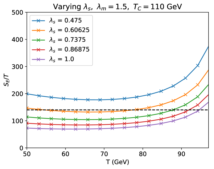
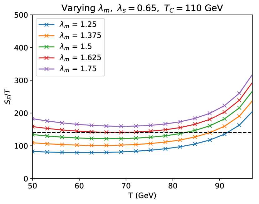
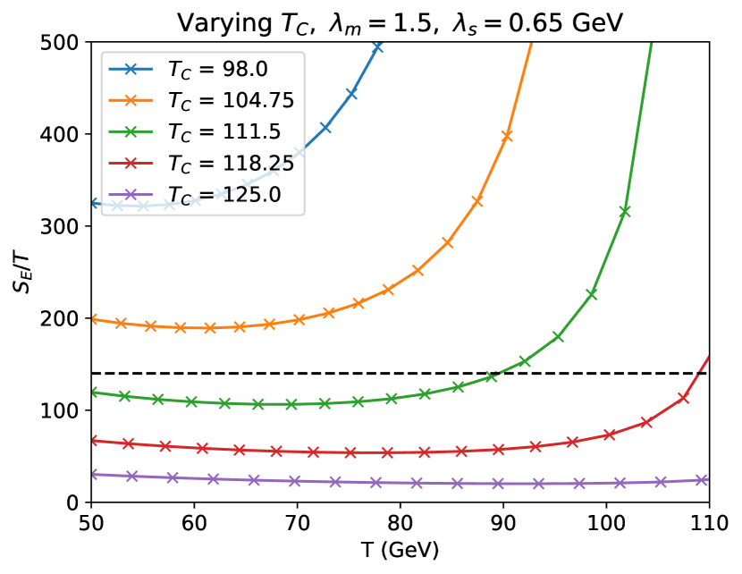
Figure 12: Change in Euclidean action as a function of temperature for points near our benchmark. We vary $\lambda_{s}$ (top left frame), $\lambda_{m}$ (top right frame) and the critical temperature, $T_{C}$ (bottom frame), relative to the base point $\{T_{C},\lambda_{m},\lambda_{s}\}=\{110\ \textrm{GeV},1.5,0.65\}$. The horizontal black dashed line represents the nucleation threshold $S_{E}/T=140$, and the intersection of a curve with this line is the nucleation temperature. For all choices of the parameters as $T$ approaches $T_{C}$, the solution becomes thin walled and $S_{E}$ approaches infinity which causes the nucleation curves to diverge, though some curves are cut off before this is visible, and will run into numerical problems associated with thin walls for temperatures close enough to $T_{c}$.

Having constructed the benchmark point, we now use BubbleProfiler to investigate the bounce action by individually varying the parameters $\{T_{C},\lambda_{m},\lambda_{s}\}$. For each parameter set, BubbleProfiler was used to solve the bounce equation for temperatures in the interval $[50\,\textrm{GeV},T_{C}]$. The change in bounce action with respect to temperature is shown in Figure 12. We mark $S_{E}(T)/T\approx 140$ by a horizontal line, showing how the nucleation temperature changes with respect to each parameter in the vicinity of the benchmark point. As was first demonstrated in Ref. [115] a very significant constraint on successful electroweak baryogenesis in this model is whether or not the bubble nucleation takes place at any finite temperature. While we do not perform a full scan, by varying about our benchmark we also find this constraint has an impact.

As can be seen in the top left frame Figure 12 if $\lambda_{s}$ is much smaller than that of the benchmark point we find no solution to Eq. 90. While our results are not directly comparable to those of Ref. [115] due to different approximations made in the calculation of the potential and slightly different criteria for bubble nucleation these findings are in qualitative agreement with their results, which are a result of smaller $\lambda_{s}$ leading to a larger height and width of the barrier in the first order phase transition. At the same time as shown in the top right frame of Figure 12 if $\lambda_{m}$ is too large then there is also no bubble nucleation, and this result is again in qualitative agreement with the findings of Ref. [115]. Finally we see in the bottom frame of Figure 12 that for our benchmark values of $\lambda_{s}$ and $\lambda_{m}$ if the critical temperature is too large then there is again no bubble nucleation. The scripts used to run these tests are distributed under the examples/sm-plus-singlet directory.

9 Conclusions

Vacuum decay appears in a wide variety of contexts in particle physics and cosmology. For example there may be fundamental symmetries, like the electroweak symmetry, that get broken in the cosmological history, and may create observable gravitational waves or generate the observed baryon asymmetry of the universe through an electroweak baryogenesis mechanism. There is also the possibility of SM extensions with deeper underlying charge or color breaking minima at zero temperature, where the possibility of the vacuum decay can place limits on the model depending on the lifetime of the metastable electroweak vacuum. Even the SM electroweak vacuum may be metastable if it is valid up to the Planck scale.

In cases where the vacuum decays by bubble nucleation, calculating the rate of vacuum decay and related properties of the transition requires solving the bounce equations to obtain the bubble profile and Euclidean action. We have described how this can be done using BubbleProfiler, a new C++ code, which is easy to use, fast and adaptable. BubbleProfiler is designed with flexibility and modularity in mind and is distributed with two methods for solving the bounce equations: a perturbative method capable of finding the bounce solution for any number of scalar fields, and a special shooting method for one-dimensional potentials. Each component in the perturbative calculation can be replaced and updated, allowing both short term adaptations and long term evolution.

We tested BubbleProfiler against existing codes, CosmoTransitions and AnyBubble, and against a number of example potentials with known analytic solutions. We found that BubbleProfiler is fast and can find the bounce solution for a $3$ field potential in under one second. For single field potentials, BubbleProfiler is the fastest of the three codes. Finally, this new code is intended to grow and develop. We strongly encourage users to give us feedback on the code, suggestions for new features, and to contact us with any questions relating to BubbleProfiler.

A Interface to bubbler solvers — bubbler

For ease of comparing results from BubbleProfiler, CosmoTransitions and AnyBubble, we make our testing suite publicly available at https://github.com/bubbleprofiler/bubbler. This is a Python interface to AnyBubble, BubbleProfiler and CosmoTransitions for solving the bounce action and plotting the profiles. This requires you to set paths to the codes

⬇

export PYTHONPATH=Absolute/Path/To/CosmoTransitions

export BUBBLEPROFILER=Absolute/Path/To/BubbleProfiler

export ANYBUBBLE=Absolute/Path/To/AnyBubble

If you only wish to use particular codes, as e.g., you have not installed one, add the keyword argument for backend, e.g., backends=["bubbleprofiler"].

To calculate the bounce actions, e.g.,

⬇

>>> from bubbler import bubblers

>>> print bubblers("0.1*((-x + 2)^4 - 14*(-x + 2)^2 + 24*(-x + 2))")

=== cosmotransitions ===

action = 52.5648686747

time = 0.272551059723

command = fullTunneling

=== anybubble ===

action = 52.3890699633

time = 6.020316

command = math -script /tmp/tmpp2sNls/anybubble.ws

=== bubbleprofiler ===

action = 54.112

time = 0.0439109802246

command = ~/BubbleProfiler/bin/run_cmd_line_potential.x --force-output --write-profiles --potential ’0.1*((-x + 2)^4 - 14*(-x + 2)^2 + 24*(-x + 2))’ --field ’x’ --output-file /tmp/tmputKUDO --initial-step-size 0.01 --domain-start -1.0 --domain-end -1.0 --local-minimum 0.0 --global-minimum 5.0 --rtol-action 0.001 --rtol-fields 0.001 --integration-method runge-kutta-4 --n-dims 3 > /dev/null 2>&1

bubblers itself returns a dictionary-like object of information about the solutions. You can select $d=4$ by the keyword argument dim = 4. The potential may be a multi-field one. For the profiles, the code

⬇

>>> from bubbler import profiles

>>> profiles("0.1*((-x + 2)^4 - 14*(-x + 2)^2 + 24*(-x + 2))")

shows the bubble profile for every field for every code.

B Multi-field polynomial potentials

We devised polynomial potentials for the purposes of testing with multiple fields. For one field, we use the potential,

$$V(x)=\frac{1}{10}\left(x^{4}-8x^{3}+10x^{2}+8\right).$$ (91)

with extrema at $x=0$, $1$ and $5$. For greater than one field, we construct potentials of the form

$$V=\left(\left[\sum_{i=1}^{n}c_{i}(x_{i}-1)^{2}\right]-c_{n+1}\right)\left(\sum_{i=1}^{n}x_{i}^{2}\right),$$ (92)

with vacua close to $x_{i}=0$ and $1$ for all $i$. Thus to construct potentials with $2$–$8$ fields, we pick the coefficients,

$$c =\left(1.8,0.2,0.3\right),$$ (93)

$$c =\left(0.684373,0.181928,0.295089,0.284821\right),$$ (94)

$$c =\left(0.534808,0.77023,0.838912,0.00517238,0.258889\right),$$ (95)

$$c =\left(0.4747,0.234808,0.57023,0.138912,0.517238,0.658889\right),$$ (96)

$$c =\left(0.34234,0.4747,0.234808,0.57023,0.138912,0.517238,0.658889\right),$$ (97)

$$c =\left(0.5233,0.34234,0.4747,0.234808,0.57023,0.138912,0.517238,0.658889\right),$$ (98)

$$c =\left(0.2434,0.5233,0.34234,0.4747,0.234808,0.57023,0.138912,0.51723,0.658889\right).$$ (99)

This form was introduced for two-dimensional potentials in Ref. [78]. The parameter $c_{n+1}$ governs the degeneracy of the vacua; for $c_{n+1}\ll 1$, the true and false vacua are almost degenerate and the bubble profile must be thin-walled.

C Command line interface

The main user interface for BubbleProfiler is the bin/run_cmd_line_potential.x tool. An example command demonstrating the minimal required inputs is:

⬇

run_cmd_line_potential.x --potential "(x^2 + y^2)*(1.8*(x - 1)^2 + 0.2*(y - 1)^2 - 0.3)" --field "x" --field "y" --false-vacuum-at-origin --global-minimum 1.0402967171 1.53520719837

which results in output

⬇

Potential: (x^2 + y^2)*(1.8*(x - 1)^2 + 0.2*(y - 1)^2 - 0.3)

Field: x

Field: y

# Action: 20.8363

A comprehensive set of options allows the user to choose which algorithms will be used to solve the bounce equations, customize relevant parameters, and specify output formats. We list these below in three groups: general options applying to all potentials, options which affect the ansatz solution, and options specific to solving single field problems with the direct shooting algorithm.

C.1 General options

--help

Print a summary of the command line options.

--potential (required):

Potential for one or more fields given in GiNaC’s [106] syntax. For example, the two field potential in equation Eq. 93 would be specified by:

⬇

--potential "(x^2 + y^2)*(1.8*(x - 1)^2 + 0.2*(y - 1)^2 - 0.3)"

--field (required):

Indicates which symbols in the potential correspond to fields. Can be specified multiple times. For example, a two field potential with fields x and y would require:

⬇

--field "x" --field "y"

--n-dims:

Number of spacetime dimensions $d$. Typically $d=4$ for zero temperature calculations, and $d=3$ at finite temperatures. Corresponds to the parameter $n$ in Section 3 via $n=d-1$.

--perturbative:

Force BubbleProfiler to always use the perturbative algorithm described in Section 5. If this option is not specified, the direct shooting method described in Section 4 will be used for single field potentials.

--global-minimum (required):

Location of the true vacuum. The potential in Eq. 93 has a true vacuum at x=1.0402967171, y=1.0402967171, which would be specified by:

⬇

--global-minimum 1.0402967171 1.0402967171

The order of the field coordinates should be the same as the –field flags. If a true vacuum is not specified, BubbleProfiler will attempt to find it using global optimization.

--opt-timeout:

Sets a time limit if finding the true vacuum using global optimization. Omitting this option, or specifying a value of $0$ results in no time limit.

--local-minimum (required):

Location of the false vacuum. Specification format is the same as for –global-minimum. Required unless the --false-vacuum-at-origin flag is given.

--false-vacuum-at-origin:

Assume that the false vacuum lies at the origin in field space.

--domain-start:

Radial coordinate for start of finite domain ($\rho_{\text{min}}$) on which bounce equations are solved. Omitting this option, or specifying a negative number will cause BubbleProfiler to guess an appropriate value. This is done by finding the point closest to the origin where the radial derivative of the ansatz solution is equal to $10^{-5}$.

--domain-end:

Radial coordinate for end of finite domain ($\rho_{\text{max}}$). Omitting --domain-end or specifying a negative value will cause BubbleProfiler to estimate a value by finding the outermost point at which the value of the ansatz solution is less than or equal to $10^{-5}$. This is usually sufficient, but in the case of ’long tailed’ solutions automatic domain sizing may cause the action to be underestimated. We recommend that users relying on automatic domain sizing for large scans take care to verify that manually increasing the domain size does not significantly change the calculated action.

--initial-step-size:

This option specifies the approximate initial step size to use in solving ODEs. When using the perturbative algorithm, a fixed step size close to this value will be used over the radial grid. The shooting algorithm uses an adaptive step size which will evolve from this initial value during integration.

--interpolation-fraction:

Approximate fraction of the total number of grid points to use when building cubic spline interpolations of intermediate solutions.

--integration-method:

Algorithm to use when integrating the perturbation equations, Eq. 48. Available options are fourth order Runge-Kutta (–integration-method=RK4) or the Euler method (–integration-method=euler).

--rtol-action, --rtol-field:

Relative tolerance criteria for determining when to halt iteration. –rtol-action is compared to the relative change in the bounce action between iterates. –rtol-fields is compared to the relative change in the starting values $\phi_{0j}=\phi_{j}(\rho_{\text{min}})$ of each field. The iteration halts when both of these quantities fall below their respective thresholds.

--max-iterations:

Maximum number of iterations to perform, regardless of convergence criteria. Omitting this option or setting it to a negative value will cause BubbleProfiler to iterate until the convergence criteria set via –rtol-action and –rtol-field are met.

--output-path:

Directory in which to store output files. Three files are created:

• action.txt File listing the Euclidean action of the solution at each iteration, up to the final profile.

• field_profiles.txt Listing of the field profiles for each iteration.

• perturbations.txt Listing of the correction functions applied at each iteration.

--force-output:

Overwrite files in the output directory. If this option is not specified and files are present, BubbleProfiler will exit with an error message.

--output-file:

Write an additional summary file at the indicated location. By default, this contains only the Euclidean action of the final solution.

--write-profiles:

Print the final set of field profiles to the console after execution. If the –output-file option is specified, the profiles will be written to the summary file instead.

--verbose

Print detailed information to the console while computing the bubble profile.

C.2 Ansatz options

By default, the parametric kink ansatz described in Section 5.1 is used to construct the initial field profiles. The following options provide alternative ansatz solutions.

--shooting-ansatz:

Use the 1D direct shooting method described in Section 4 to construct the initial profiles. Note that the options described in Section C.3 will affect the calculation of this ansatz.

--ansatz-file:

Load a precomputed ansatz from a text file. Each row consists of a radial field coordinate $\rho_{j}$, followed by the field values $\phi_{i}(\rho_{j})$. Columns are separated by spaces. The order in which the fields appear must match the –field specifications, and the radial coordinates $\rho_{j}$ must match the discrete grid representation to a tolerance of $10^{-6}$, if a grid has already been given. An example using a textfile ansatz is provided in the examples/textfile-ansatz directory.

C.3 Options specific to single field direct shooting

The following options will only have an effect on the behavior of BubbleProfiler when solving single field problems using the direct shooting method.

--barrier:

Specify the location of the barrier separating the true and false vacua. If not supplied, BubbleProfiler will attempt to find the barrier numerically.

--action-arrived-rel:

Relative tolerance for arriving at the false vacuum when calculating bounce action.

--shoot-ode-abs, --shoot-ode-rel:

Absolute and relative error tolerances for ODE integrator when calculating bubble profile.

--action-ode-abs, --action-ode-rel:

Absolute and relative error tolerances for ODE integrator when calculating bounce action.

--drho-frac:

Initial step size relative to characteristic bubble scale (Eq. 29).

--evolve-change-rel:

How far to evolve using approximate analytic solutions (Eq. 23 and Eq. 24) in terms of change in field value relative to difference between true and false vacua. Corresponds to the $f$ parameter in Eq. 25.

--bisect-lambda-max:

Maximum value of bisection parameter $\lambda$ (Eq. 30).

--iter-max:

Maximum number of iterations of the shooting method.

--periods-max:

Evolve the field for a maximum of this number of multiples of the characteristic bubble scale (Eq. 29).

--f-y-max:

As discussed in Section 4.1, we evolve the field analytically until it changes by a specified fraction. This involves evaluating complicated functions, such as inverse sinc and hyperbolic sinc, at $t$ (defined in Eq. 27). If $t>\text{\nolinkurl{f_y_max}}$, we instead use an asymptotic approximation for the critical time and velocity at that time.

--f-y-min:

Similar to the –f-y-max argument: if $t<\text{\nolinkurl{f_y_min}}$, we use an asymptotic approximation for the velocity at the critical time.

--y-max:

Similar to the –f-y-max argument: we find the action for the interior of the bubble, before the field changes by a specified fraction, analytically. If $m\hat{\rho}>\text{\nolinkurl{y_max}}$, we use a simpler asymptotic approximation for it.

References

- [1] S. R. Coleman, The Fate of the False Vacuum. 1. Semiclassical Theory, Phys. Rev. D15 (1977) 2929–2936.
- [2] C. G. Callan, Jr. and S. R. Coleman, The Fate of the False Vacuum. 2. First Quantum Corrections, Phys. Rev. D16 (1977) 1762–1768.
- [3] A. D. Linde, Fate of the False Vacuum at Finite Temperature: Theory and Applications, Phys. Lett. 100B (1981) 37–40.
- [4] D. E. Morrissey and M. J. Ramsey-Musolf, Electroweak baryogenesis, New J. Phys. 14 (2012) 125003, [1206.2942].
- [5] G. A. White, A Pedagogical Introduction to Electroweak Baryogenesis. IOP Concise Physics. Morgan & Claypool, 2016, 10.1088/978-1-6817-4457-5.
- [6] A. K. Das, Topics in finite temperature field theory, hep-ph/0004125.
- [7] C. Lee, V. Cirigliano and M. J. Ramsey-Musolf, Resonant relaxation in electroweak baryogenesis, Phys. Rev. D71 (2005) 075010, [hep-ph/0412354].
- [8] C. Balazs, M. Carena, A. Menon, D. E. Morrissey and C. E. M. Wagner, The Supersymmetric origin of matter, Phys. Rev. D71 (2005) 075002, [hep-ph/0412264].
- [9] M. Carena, G. Nardini, M. Quiros and C. E. M. Wagner, The Baryogenesis Window in the MSSM, Nucl. Phys. B812 (2009) 243–263, [0809.3760].
- [10] M. Carena, G. Nardini, M. Quiros and C. E. M. Wagner, MSSM Electroweak Baryogenesis and LHC Data, JHEP 02 (2013) 001, [1207.6330].
- [11] S. Liebler, S. Profumo and T. Stefaniak, Light Stop Mass Limits from Higgs Rate Measurements in the MSSM: Is MSSM Electroweak Baryogenesis Still Alive After All?, JHEP 04 (2016) 143, [1512.09172].
- [12] S. J. Huber, P. John and M. G. Schmidt, Bubble walls, CP violation and electroweak baryogenesis in the MSSM, Eur. Phys. J. C20 (2001) 695–711, [hep-ph/0101249].
- [13] S. J. Huber, T. Konstandin, T. Prokopec and M. G. Schmidt, Baryogenesis in the MSSM, nMSSM and NMSSM, Nucl. Phys. A785 (2007) 206–209, [hep-ph/0608017].
- [14] A. Menon, D. E. Morrissey and C. E. M. Wagner, Electroweak baryogenesis and dark matter in the nMSSM, Phys. Rev. D70 (2004) 035005, [hep-ph/0404184].
- [15] C. Balázs, A. Mazumdar, E. Pukartas and G. White, Baryogenesis, dark matter and inflation in the Next-to-Minimal Supersymmetric Standard Model, JHEP 01 (2014) 073, [1309.5091].
- [16] S. Akula, C. Balázs, L. Dunn and G. White, Electroweak baryogenesis in the -invariant NMSSM, JHEP 11 (2017) 051, [1706.09898].
- [17] A. T. Davies, C. D. Froggatt and R. G. Moorhouse, Electroweak baryogenesis in the next-to-minimal supersymmetric model, Phys. Lett. B372 (1996) 88–94, [hep-ph/9603388].
- [18] S. J. Huber, T. Konstandin, T. Prokopec and M. G. Schmidt, Electroweak Phase Transition and Baryogenesis in the nMSSM, Nucl. Phys. B757 (2006) 172–196, [hep-ph/0606298].
- [19] J. Kozaczuk, S. Profumo, L. S. Haskins and C. L. Wainwright, Cosmological Phase Transitions and their Properties in the NMSSM, JHEP 01 (2015) 144, [1407.4134].
- [20] L. Bian, H.-K. Guo and J. Shu, Gravitational Waves, baryon asymmetry of the universe and electric dipole moment in the CP-violating NMSSM, 1704.02488.
- [21] M. J. Ramsey-Musolf, G. White and P. Winslow, Color Breaking Baryogenesis, 1708.07511.
- [22] S. Inoue, G. Ovanesyan and M. J. Ramsey-Musolf, Two-Step Electroweak Baryogenesis, Phys. Rev. D93 (2016) 015013, [1508.05404].
- [23] H. H. Patel, M. J. Ramsey-Musolf and M. B. Wise, Color Breaking in the Early Universe, Phys. Rev. D88 (2013) 015003, [1303.1140].
- [24] C. Balazs, G. White and J. Yue, Effective field theory, electric dipole moments and electroweak baryogenesis, JHEP 03 (2017) 030, [1612.01270].
- [25] J. de Vries, M. Postma, J. van de Vis and G. White, Electroweak Baryogenesis and the Standard Model Effective Field Theory, JHEP 01 (2018) 089, [1710.04061].
- [26] C. Grojean, G. Servant and J. D. Wells, First-order electroweak phase transition in the standard model with a low cutoff, Phys. Rev. D71 (2005) 036001, [hep-ph/0407019].
- [27] A. Kobakhidze, L. Wu and J. Yue, Electroweak Baryogenesis with Anomalous Higgs Couplings, JHEP 04 (2016) 011, [1512.08922].
- [28] F. P. Huang, P.-H. Gu, P.-F. Yin, Z.-H. Yu and X. Zhang, Testing the electroweak phase transition and electroweak baryogenesis at the LHC and a circular electron-positron collider, Phys. Rev. D93 (2016) 103515, [1511.03969].
- [29] H. H. Patel and M. J. Ramsey-Musolf, Baryon Washout, Electroweak Phase Transition, and Perturbation Theory, JHEP 07 (2011) 029, [1101.4665].
- [30] Virgo, LIGO Scientific collaboration, B. P. Abbott et al., Observation of Gravitational Waves from a Binary Black Hole Merger, Phys. Rev. Lett. 116 (2016) 061102, [1602.03837].
- [31] D. Croon and G. White, Exotic Gravitational Wave Signatures from Simultaneous Phase Transitions, 1803.05438.
- [32] K. Hashino, M. Kakizaki, S. Kanemura, P. Ko and T. Matsui, Gravitational waves from first order electroweak phase transition in models with the gauge symmetry, 1802.02947.
- [33] M. Chala, C. Krause and G. Nardini, Signals of the electroweak phase transition at colliders and gravitational wave observatories, 1802.02168.
- [34] Y. Chen, M. Huang and Q.-S. Yan, Gravitation waves from QCD and electroweak phase transitions, 1712.03470.
- [35] Z. Kang, P. Ko and T. Matsui, Strong first order EWPT & strong gravitational waves in Z3-symmetric singlet scalar extension, JHEP 02 (2018) 115, [1706.09721].
- [36] S. Iso, P. D. Serpico and K. Shimada, QCD-Electroweak First-Order Phase Transition in a Supercooled Universe, Phys. Rev. Lett. 119 (2017) 141301, [1704.04955].
- [37] A. Kobakhidze, C. Lagger, A. Manning and J. Yue, Gravitational waves from a supercooled electroweak phase transition and their detection with pulsar timing arrays, Eur. Phys. J. C77 (2017) 570, [1703.06552].
- [38] A. Beniwal, M. Lewicki, J. D. Wells, M. White and A. G. Williams, Gravitational wave, collider and dark matter signals from a scalar singlet electroweak baryogenesis, JHEP 08 (2017) 108, [1702.06124].
- [39] W. Chao, H.-K. Guo and J. Shu, Gravitational Wave Signals of Electroweak Phase Transition Triggered by Dark Matter, JCAP 1709 (2017) 009, [1702.02698].
- [40] F. P. Huang, Y. Wan, D.-G. Wang, Y.-F. Cai and X. Zhang, Hearing the echoes of electroweak baryogenesis with gravitational wave detectors, Phys. Rev. D94 (2016) 041702, [1601.01640].
- [41] F. P. Huang and J.-H. Yu, Exploring inert dark matter blind spots with gravitational wave signatures, Phys. Rev. D98 (2018) 095022, [1704.04201].
- [42] M. Chala, M. Ramos and M. Spannowsky, Gravitational wave and collider probes of extended Higgs sectors with a low cutoff, 1812.01901.
- [43] A. Angelescu and P. Huang, Multistep Strongly First Order Phase Transitions from New Fermions at the TeV Scale, 1812.08293.
- [44] P. Schwaller, Gravitational Waves from a Dark Phase Transition, Phys. Rev. Lett. 115 (2015) 181101, [1504.07263].
- [45] J. Shelton and K. M. Zurek, Darkogenesis: A baryon asymmetry from the dark matter sector, Phys. Rev. D82 (2010) 123512, [1008.1997].
- [46] T. A. Chowdhury, M. Nemevsek, G. Senjanovic and Y. Zhang, Dark Matter as the Trigger of Strong Electroweak Phase Transition, JCAP 1202 (2012) 029, [1110.5334].
- [47] D. Croon, V. Sanz and G. White, Model Discrimination in Gravitational Wave spectra from Dark Phase Transitions, JHEP 08 (2018) 203, [1806.02332].
- [48] S. J. Huber and T. Konstandin, Production of gravitational waves in the nMSSM, JCAP 0805 (2008) 017, [0709.2091].
- [49] C. Balazs, A. Fowlie, A. Mazumdar and G. White, Gravitational waves at aLIGO and vacuum stability with a scalar singlet extension of the Standard Model, Phys. Rev. D95 (2017) 043505, [1611.01617].
- [50] M. Kamionkowski, A. Kosowsky and M. S. Turner, Gravitational radiation from first order phase transitions, Phys. Rev. D49 (1994) 2837–2851, [astro-ph/9310044].
- [51] R. Apreda, M. Maggiore, A. Nicolis and A. Riotto, Gravitational waves from electroweak phase transitions, Nucl. Phys. B631 (2002) 342–368, [gr-qc/0107033].
- [52] C. Caprini, R. Durrer and G. Servant, Gravitational wave generation from bubble collisions in first-order phase transitions: An analytic approach, Phys. Rev. D77 (2008) 124015, [0711.2593].
- [53] M. Hindmarsh, S. J. Huber, K. Rummukainen and D. J. Weir, Gravitational waves from the sound of a first order phase transition, Phys. Rev. Lett. 112 (2014) 041301, [1304.2433].
- [54] C. Caprini, R. Durrer, T. Konstandin and G. Servant, General Properties of the Gravitational Wave Spectrum from Phase Transitions, Phys. Rev. D79 (2009) 083519, [0901.1661].
- [55] J. R. Espinosa, T. Konstandin, J. M. No and G. Servant, Energy Budget of Cosmological First-order Phase Transitions, JCAP 1006 (2010) 028, [1004.4187].
- [56] P. Binetruy, A. Bohe, C. Caprini and J.-F. Dufaux, Cosmological Backgrounds of Gravitational Waves and eLISA/NGO: Phase Transitions, Cosmic Strings and Other Sources, JCAP 1206 (2012) 027, [1201.0983].
- [57] F. P. Huang and X. Zhang, Probing the gauge symmetry breaking of the early universe in 3-3-1 models and beyond by gravitational waves, Phys. Lett. B788 (2019) 288–294, [1701.04338].
- [58] Y. Wan, B. Imtiaz and Y.-F. Cai, Cosmological phase transitions and gravitational waves in the singlet Majoron model, 1804.05835.
- [59] A. Mazumdar and G. White, Cosmic phase transitions: their applications and experimental signatures, 1811.01948.
- [60] D. Croon, T. E. Gonzalo and G. White, Gravitational Waves from a Pati-Salam Phase Transition, 1812.02747.
- [61] S. J. Huber and T. Konstandin, Gravitational Wave Production by Collisions: More Bubbles, JCAP 0809 (2008) 022, [0806.1828].
- [62] M. Hindmarsh, S. J. Huber, K. Rummukainen and D. J. Weir, Shape of the acoustic gravitational wave power spectrum from a first order phase transition, Phys. Rev. D96 (2017) 103520, [1704.05871].
- [63] R. Jinno and M. Takimoto, Gravitational waves from bubble dynamics: Beyond the Envelope, 1707.03111.
- [64] M. Hindmarsh, Sound shell model for acoustic gravitational wave production at a first-order phase transition in the early Universe, Phys. Rev. Lett. 120 (2018) 071301, [1608.04735].
- [65] T. Konstandin, Gravitational radiation from a bulk flow model, JCAP 1803 (2018) 047, [1712.06869].
- [66] D. J. Weir, Gravitational waves from a first order electroweak phase transition: a brief review, Phil. Trans. Roy. Soc. Lond. A376 (2018) 20170126, [1705.01783].
- [67] M. Sher, Electroweak Higgs Potentials and Vacuum Stability, Phys. Rept. 179 (1989) 273–418.
- [68] J. E. Camargo-Molina, B. O’Leary, W. Porod and F. Staub, Stability of the CMSSM against sfermion VEVs, JHEP 12 (2013) 103, [1309.7212].
- [69] N. Blinov and D. E. Morrissey, Vacuum Stability and the MSSM Higgs Mass, JHEP 03 (2014) 106, [1310.4174].
- [70] B. Swiezewska, Inert scalars and vacuum metastability around the electroweak scale, JHEP 07 (2015) 118, [1503.07078].
- [71] M. Bobrowski, G. Chalons, W. G. Hollik and U. Nierste, Vacuum stability of the effective Higgs potential in the Minimal Supersymmetric Standard Model, Phys. Rev. D90 (2014) 035025, [1407.2814].
- [72] W. G. Hollik, A new view on vacuum stability in the MSSM, JHEP 08 (2016) 126, [1606.08356].
- [73] J. E. Camargo-Molina, B. O’Leary, W. Porod and F. Staub, On the vacuum stability of SUSY models, PoS EPS-HEP2013 (2013) 265, [1310.1260].
- [74] A. Andreassen, W. Frost and M. D. Schwartz, Scale Invariant Instantons and the Complete Lifetime of the Standard Model, Phys. Rev. D97 (2018) 056006, [1707.08124].
- [75] G. Degrassi, S. Di Vita, J. Elias-Miro, J. R. Espinosa, G. F. Giudice, G. Isidori et al., Higgs mass and vacuum stability in the Standard Model at NNLO, JHEP 08 (2012) 098, [1205.6497].
- [76] L. Delle Rose, C. Marzo and A. Urbano, On the fate of the Standard Model at finite temperature, JHEP 05 (2016) 050, [1507.06912].
- [77] P. Basler and M. Mühlleitner, BSMPT - Beyond the Standard Model Phase Transitions -A Tool for the Electroweak Phase Transition in Extended Higgs Sectors, 1803.02846.
- [78] C. L. Wainwright, CosmoTransitions: Computing Cosmological Phase Transition Temperatures and Bubble Profiles with Multiple Fields, Comput. Phys. Commun. 183 (2012) 2006–2013, [1109.4189].
- [79] J. E. Camargo-Molina, B. O’Leary, W. Porod and F. Staub, : A Tool For Finding The Global Minima Of One-Loop Effective Potentials With Many Scalars, Eur. Phys. J. C73 (2013) 2588, [1307.1477].
- [80] A. Masoumi, K. D. Olum and B. Shlaer, Efficient numerical solution to vacuum decay with many fields, JCAP 1701 (2017) 051, [1610.06594].
- [81] M. Claudson, L. J. Hall and I. Hinchliffe, Low-Energy Supergravity: False Vacua and Vacuous Predictions, Nucl. Phys. B228 (1983) 501–528.
- [82] A. Kusenko, Improved action method for analyzing tunneling in quantum field theory, Phys. Lett. B358 (1995) 51–55, [hep-ph/9504418].
- [83] A. Kusenko, P. Langacker and G. Segre, Phase transitions and vacuum tunneling into charge and color breaking minima in the MSSM, Phys. Rev. D54 (1996) 5824–5834, [hep-ph/9602414].
- [84] J. M. Moreno, M. Quiros and M. Seco, Bubbles in the supersymmetric standard model, Nucl. Phys. B526 (1998) 489–500, [hep-ph/9801272].
- [85] P. John, Bubble wall profiles with more than one scalar field: A Numerical approach, Phys. Lett. B452 (1999) 221–226, [hep-ph/9810499].
- [86] J. M. Cline, G. D. Moore and G. Servant, Was the electroweak phase transition preceded by a color broken phase?, Phys. Rev. D60 (1999) 105035, [hep-ph/9902220].
- [87] I. Dasgupta, Estimating vacuum tunneling rates, Phys. Lett. B394 (1997) 116–122, [hep-ph/9610403].
- [88] J. M. Cline, J. R. Espinosa, G. D. Moore and A. Riotto, String mediated electroweak baryogenesis: A Critical analysis, Phys. Rev. D59 (1999) 065014, [hep-ph/9810261].
- [89] T. Konstandin and S. J. Huber, Numerical approach to multi dimensional phase transitions, JCAP 0606 (2006) 021, [hep-ph/0603081].
- [90] V. Guada, A. Maiezza and M. Nemevšek, Polygonal bounces, 1803.02227.
- [91] J. R. Espinosa, A Fresh Look at the Calculation of Tunneling Actions, 1805.03680.
- [92] J. R. Espinosa and T. Konstandin, A Fresh Look at the Calculation of Tunneling Actions in Multi-Field Potentials, 1811.09185.
- [93] R. Jinno, Machine learning for bounce calculation, 1805.12153.
- [94] S. Akula, C. Balázs and G. A. White, Semi-analytic techniques for calculating bubble wall profiles, Eur. Phys. J. C76 (2016) 681, [1608.00008].
- [95] V. Cirigliano, C. Lee, M. J. Ramsey-Musolf and S. Tulin, Flavored Quantum Boltzmann Equations, Phys. Rev. D81 (2010) 103503, [0912.3523].
- [96] V. Cirigliano, C. Lee and S. Tulin, Resonant Flavor Oscillations in Electroweak Baryogenesis, Phys. Rev. D84 (2011) 056006, [1106.0747].
- [97] K. Kainulainen, T. Prokopec, M. G. Schmidt and S. Weinstock, First principle derivation of semiclassical force for electroweak baryogenesis, JHEP 06 (2001) 031, [hep-ph/0105295].
- [98] D. J. H. Chung, B. Garbrecht, M. Ramsey-Musolf and S. Tulin, Supergauge interactions and electroweak baryogenesis, JHEP 12 (2009) 067, [0908.2187].
- [99] G. A. White, General analytic methods for solving coupled transport equations: From cosmology to beyond, Phys. Rev. D93 (2016) 043504, [1510.03901].
- [100] A. D. Linde, Decay of the False Vacuum at Finite Temperature, Nucl. Phys. B216 (1983) 421.
- [101] S. R. Coleman, Quantum Tunneling and Negative Eigenvalues, Nucl. Phys. B298 (1988) 178–186.
- [102] J. Dormand and P. Prince, A family of embedded Runge-Kutta formulae, Journal of Computational and Applied Mathematics 6 (1980) 19 – 26.
- [103] L. V. Kantorovich, Functional analysis and applied mathematics, Uspekhi Math. Nauk 3 (1948) 89–185.
- [104] W. T. Vetterling, Numerical Recipes Example Book C++: The Art of Scientific Computing. CreateSpace Independent Publishing Platform, Aug., 2017.
- [105] M. Baake and U. Schlägel, The Peano-Baker series, Proceedings of the Steklov Institute of Mathematics 275 (Dec., 2011) 155–159.
- [106] C. Bauer, A. Frink and R. Kreckel, Introduction to the GiNaC Framework for Symbolic Computation within the C++ Programming Language, Journal of Symbolic Computation 33 (Jan., 2002) 1–12.
- [107] “NLOpt optimisation library.” https://nlopt.readthedocs.io/en/latest/, 2018.
- [108] “Eigen3 fast numerical linear algebra library.” http://eigen.tuxfamily.org/index.php?title=Main_Page, 2018.
- [109] “GSL — GNU scientific library.” https://www.gnu.org/software/gsl/, 2018.
- [110] A. Aravind, B. S. DiNunno, D. Lorshbough and S. Paban, Analyzing multifield tunneling with exact bounce solutions, Phys. Rev. D91 (2015) 025026, [1412.3160].
- [111] GAMBIT collaboration, P. Athron et al., Status of the scalar singlet dark matter model, Eur. Phys. J. C77 (2017) 568, [1705.07931].
- [112] P. Athron, J. M. Cornell, F. Kahlhoefer, J. Mckay, P. Scott and S. Wild, Impact of vacuum stability, perturbativity and XENON1T on global fits of and scalar singlet dark matter, Eur. Phys. J. C78 (2018) 830, [1806.11281].
- [113] J. McDonald, Gauge singlet scalars as cold dark matter, Physical Review D 50 (Sept., 1994) 3637–3649.
- [114] C. P. Burgess, M. Pospelov and T. ter Veldhuis, The Minimal Model of nonbaryonic dark matter: A singlet scalar, Nuclear Physics B 619 (Dec., 2001) 709–728.
- [115] G. Kurup and M. Perelstein, Dynamics of Electroweak Phase Transition In Singlet-Scalar Extension of the Standard Model, Physical Review D 96 (July, 2017) , [1704.03381].
- [116] J. M. Cline and K. Kainulainen, Electroweak baryogenesis and dark matter from a singlet Higgs, Journal of Cosmology and Astroparticle Physics 2013 (2013) 012.
- [117] V. Vaskonen, Electroweak baryogenesis and gravitational waves from a real scalar singlet, Phys. Rev. D95 (2017) 123515, [1611.02073].
- [118] J. R. Espinosa, T. Konstandin and F. Riva, Strong Electroweak Phase Transitions in the Standard Model with a Singlet, Nuclear Physics B 854 (Jan., 2012) 592–630, [1107.5441].
- [119] ATLAS, CMS collaboration, G. Aad et al., Measurements of the Higgs boson production and decay rates and constraints on its couplings from a combined ATLAS and CMS analysis of the LHC pp collision data at and 8 TeV, JHEP 08 (2016) 045, [1606.02266].