Open quantum system in external magnetic field within non-Markovian quantum Langevin approach

Abstract

The non-Markovian dynamics of a charged particle linearly coupled to a neutral bosonic heat bath is investigated in an external uniform magnetic field. The analytical expressions for the time-dependent and asymptotic friction and diffusion coefficients, cyclotron frequencies, variances of the coordinate and momentum, and orbital magnetic moments are derived. The role of magnetic field in the dissipation and diffusion processes is illustrated by several examples in the low- and high-temperature regimes. The localization phenomenon for a charged particle is observed. The orbital diamagnetism of quantum system in a dissipative environment is studied. The quantization conditions are found for the angular momentum.

I Introduction

The problem of description of a two-dimensional quantum system under the influence of external magnetic and electric fields and energy exchange with its environment is of great interest in atomic, nuclear, and plasma physics, astrophysics, condensed matter physics, quantum optics, and quantum information and measurement theories knigaMenskogo ; Fried ; Chuvil ; PS ; Naz ; Naz2 ; Langer ; Ginz . The intensive investigations deal with the impact of the external magnetic field on such systems as quantum dots, quantum wires, and two-dimensional electronic systems PS . The characteristics of plasma in the homogeneous external field has also importance in the physics of gas discharge Ginz .

The external fields modify the distribution of internal energy which in turn modifies or alters the electronic properties such as the carrier concentration, direction, and mobility. Modeling electric current implies the determination of the time-dependence of the number of electrons with given momentum at a certain location. The equations of motion can be obtained by using the quantum Langevin approach or density matrix formalism which is widely applied to find the effects of fluctuations and dissipation in macroscopic systems Kampen1 ; Kampen2 ; Kampen3 ; Kampen4 ; Kampen5 ; Kampen6 ; LEG ; Dodonov ; DM ; Hu1 ; Hu2 ; Ma ; Katia ; Isar ; Ford ; Ford1 ; In ; M110 ; Kanokov ; Kanokov2 ; PA ; Lac11 ; Lac13 ; Lac14 . Using the phenomenological Markovian Fokker-Planck equation for the Wigner probability function, the problem of quantum description of the damped isotropic two-dimensional harmonic oscillator in an uniform magnetic field has been studied in Ref. Dodonov in the case of arbitrary relations between the proper oscillator frequency, damping coefficients and temperature. The relations between the phenomenological diffusion coefficients ensuring the positivity of the reduced density matrix at each moment of time have been obtained in Ref. Dodonov . By including the magnetic field in the quantum non-Markovian Langevin equation, the effects of dissipation and magnetic field on localization of a charged particle moving in a confined potential have been investigated in Refs. Ford ; Ford1 . As found, the weak dissipation delocalizes the oscillation of a charged particle when the magnetic field is stronger than a certain critical value Ford1 . For a charged particle moving in a two-dimensional harmonic oscillator and an uniform magnetic field, the time-dependent friction and diffusion coefficients have been analytically derived and numerically studied within the non-Markovian quantum Langevin formalism in Ref. Kanokov2 ; PA . A charged particle moving in a static external magnetic field (without a confined potential) and linearly coupled to a heat bath has been only treated in Refs. Ma ; In , where a fully dynamical calculation of the orbital diamagnetism has been presented. In Ref. Ma The non-Markovian and Markovian Langevin formalism have been used in Refs. In and Ma , respectively. In all cases Ma ; Ford ; Ford1 ; In ; Kanokov2 , the magnetic field affects neither the memory function nor the random force appearing in the quantum Langevin equation.

The aim of the present work is to derive the analytical by the transport coefficients for a unconfined charged particle in an uniform magnetic field and dissipative environment and to study the influence of the magnetic field on these coefficients, fluctuations, cyclotron frequencies, and orbital magnetic moment (orbital diamagnetism). The paper is organized as follows. In Sec. II, we give the Hamiltonian of the system and solve the quantum non-Markovian two-dimensional Langevin equations for a charged particle moving in the plane normal to the applied field. The transport coefficients are obtained by considering the first and second moments of the stochastic dissipative equations. The discussions and illustrative numerical results are presented in Sec. III. A summary is given in Sec. IV.

II Linear coupling in coordinate with heat bath

II.1 Derivation of quantum Langevin equations

Let us consider a two-dimensional motion of a charged quantum particle in the presence of heat bath and external constant magnetic field ${\bf B}=(0,0,B)$. The total Hamiltonian of this system is Ford ; PA

$$H=H_{c}+H_{b}+H_{cb}.$$ (1)

The Hamiltonian $H_{c}$ describes the charged quantum particle with effective mass tensor and charge $e=|e|$ in magnetic field:

$$H_{c}=\frac{1}{2m_{x}}[p_{x}-eA_{x}(x,y)]^{2}+\frac{1}{2m_{y}}[p_{y}-eA_{y}(x,y)]^{2}=\frac{\pi_{x}^{2}}{2m_{x}}+\frac{\pi_{y}^{2}}{2m_{y}}.$$ (2)

Here, $m_{x}$ and $m_{y}$ are the components of the effective mass tensor, ${\bf R}=(x,y,0)$ and ${\bf p}=(p_{x},p_{y},0)$ are the coordinate and canonically conjugated momentum, respectively, ${\bf A}=(-\frac{1}{2}yB,\frac{1}{2}xB,0)$ is the vector potential of the magnetic field. For simplicity, in Eq. (2) we introduce the notations

$$\pi_{x}=p_{x}+\frac{1}{2}m_{x}\omega_{cx}y,\hskip 21.68121pt\pi_{y}=p_{y}-\frac{1}{2}m_{y}\omega_{cy}x$$

with frequencies $\omega_{cx}=\frac{eB}{m_{x}}$ and $\omega_{cy}=\frac{eB}{m_{y}}$. The cyclotron frequency is $\omega_{c}=\sqrt{\omega_{cx}\omega_{cy}}=\frac{eB}{\sqrt{m_{x}m_{y}}}$.

The second term in Eq. (1) represents the Hamiltonian of the phonon (bosonic) heat bath,

$$H_{b}=\sum_{\nu}\hbar\omega_{\nu}b_{\nu}^{+}b_{\nu},$$ (3)

where $b_{\nu}^{+}$ and $b_{\nu}$ are the phonon creation and annihilation operators of the heat bath. The coupling between the heat bath and charged particle is described by

$$H_{cb} = \sum_{\nu}(\alpha_{\nu}x+\beta_{\nu}y)(b_{\nu}^{+}+b_{\nu})+\sum_{\nu}\frac{1}{\hbar\omega_{\nu}}(\alpha_{\nu}x+\beta_{\nu}y)^{2},$$ (4)

where $\alpha_{\nu}$ and $\beta_{\nu}$ are the real coupling constants. Equation (4) is already used in literature Ma ; Ford ; In ; Kanokov2 ; PA . The first term of $H_{cb}$ in Eq. (4) corresponds to the energy exchange between the charged particle and heat bath. We introduce the counter-term (second term) in $H_{cb}$ in order to compensate the coupling-induced potential. In general case, $\alpha_{\nu}$ and $\beta_{\nu}$ depend on the strength of magnetic field and an impact of the magnetic field $\bf B$ is entered into the dissipative kernels and random forces.

The equations of motion are

$$\dot{x}(t) = \frac{i}{\hbar}[H,x]=\frac{\pi_{x}(t)}{m_{x}},\hskip 21.68121pt\dot{y}(t)=\frac{i}{\hbar}[H,y]=\frac{\pi_{y}(t)}{m_{y}},$$

$$\dot{\pi}_{x}(t) = \frac{i}{\hbar}[H,\pi_{x}]=\omega_{cy}\pi_{y}(t)-\sum_{\nu}\alpha_{\nu}(b_{\nu}^{+}(t)+b_{\nu}(t))-2\sum_{\nu}\frac{\alpha_{\nu}(\alpha_{\nu}x(t)+\beta_{\nu}y(t))}{\hbar\omega_{\nu}},$$

$$\dot{\pi}_{y}(t) = \frac{i}{\hbar}[H,\pi_{y}]=-\omega_{cx}\pi_{x}(t)-\sum_{\nu}\beta_{\nu}(b_{\nu}^{+}(t)+b_{\nu}(t))-2\sum_{\nu}\frac{\beta_{\nu}(\alpha_{\nu}x(t)+\beta_{\nu}y(t))}{\hbar\omega_{\nu}},$$ (5)

and

$$\dot{b}_{\nu}^{+}(t) = \frac{i}{\hbar}[H,b_{\nu}^{+}]=i\omega_{\nu}b_{\nu}^{+}(t)+\frac{i}{\hbar}(\alpha_{\nu}x(t)+\beta_{\nu}y(t)),$$

$$\dot{b}_{\nu}(t) = \frac{i}{\hbar}[H,b_{\nu}]=-i\omega_{\nu}b_{\nu}(t)-\frac{i}{\hbar}(\alpha_{\nu}x(t)+\beta_{\nu}y(t)).$$ (6)

The solution of Eqs. (6) are

$$b_{\nu}^{+}(t)+b_{\nu}(t) = f^{+}_{\nu}(t)+f_{\nu}(t)-\frac{2(\alpha_{\nu}x(t)+\beta_{\nu}y(t))}{\hbar\omega_{\nu}}+\frac{2}{\hbar\omega_{\nu}}\int\limits_{0}^{t}d\tau(\alpha_{\nu}{\dot{x}}(\tau)+\beta_{\nu}{\dot{y}}(\tau))\cos(\omega_{\nu}[t-\tau]),$$

$$b_{\nu}^{+}(t)-b_{\nu}(t) = f^{+}_{\nu}(t)-f_{\nu}(t)+\frac{2i}{\hbar\omega_{\nu}}\int\limits_{0}^{t}d\tau(\alpha_{\nu}{\dot{x}}(\tau)+\beta_{\nu}{\dot{y}}(\tau))\sin(\omega_{\nu}[t-\tau]),$$ (7)

where

$$f_{\nu}(t)=\left[b_{\nu}(0)+\frac{\alpha_{\nu}x(0)+\beta_{\nu}y(0)}{\hbar\omega_{\nu}}\right]e^{-i\omega_{\nu}t}.$$

Substituting (7) into (5) and eliminating the bath variables from the equations of motion for the charged particle, we obtain the set of nonlinear integro-differential stochastic dissipative equations

$$\dot{x}(t) = \frac{\pi_{x}(t)}{m_{x}},\hskip 21.68121pt\dot{y}(t)=\frac{\pi_{y}(t)}{m_{y}},$$

$$\dot{\pi}_{x}(t) = \omega_{cy}\pi_{y}(t)-\int\limits_{0}^{t}d\tau K_{xx}(t,\tau)\dot{x}(\tau)-\int\limits_{0}^{t}d\tau K_{xy}(t,\tau)\dot{x}(\tau)+F_{x}(t),$$

$$\dot{\pi}_{y}(t) = -\omega_{cx}\pi_{x}(t)-\int\limits_{0}^{t}d\tau K_{yy}(t,\tau)\dot{y}(\tau)-\int\limits_{0}^{t}d\tau K_{yx}(t,\tau)\dot{y}(\tau)+F_{y}(t).$$ (8)

The dissipative kernels and random forces in (8) are

$$K_{xx}(t,\tau) = 2\sum_{\nu}\frac{\alpha_{\nu}^{2}}{\hbar\omega_{\nu}}\cos(\omega_{\nu}[t-\tau]),$$

$$K_{xy}(t,\tau) = K_{yx}(t,\tau)=2\sum_{\nu}\frac{\alpha_{\nu}\beta_{\nu}}{\hbar\omega_{\nu}}\cos(\omega_{\nu}[t-\tau]),$$

$$K_{yy}(t,\tau) = \sum_{\nu}\frac{\beta_{\nu}^{2}}{\hbar\omega_{\nu}}\cos(\omega_{\nu}[t-\tau])$$ (9)

and

$$F_{x}(t) = \sum_{\nu}{}F_{x}^{\nu}(t)=-\sum_{\nu}{}\alpha_{\nu}[f_{\nu}^{+}(t)+f_{\nu}(t)],$$

$$F_{y}(t) = \sum_{\nu}{}F_{y}^{\nu}(t)=-\sum_{\nu}{}\beta_{\nu}[f_{\nu}^{+}(t)+f_{\nu}(t)],$$ (10)

respectively. Following the standard procedure of statistical mechanics, we identify the operators $F_{x}^{\nu}$ and $F_{y}^{\nu}$ as fluctuations because of uncertainty of the initial conditions for the bath operators. To specify the statistical properties of the fluctuations, we consider an ensemble of initial states in which the fluctuations have the Gaussian distribution with zero average value

$$\ll F^{\nu}_{x}(t)\gg=\ll F^{\nu}_{y}(t)\gg=0.$$ (11)

Here, the symbol $\ll...\gg$ denotes the average over the bath with the Bose-Einstein statistics

$$\ll f_{\nu}^{+}(t)f_{\nu^{\prime}}^{+}(t^{\prime})\gg = \ll f_{\nu}(t)f_{\nu^{\prime}}(t^{\prime})\gg=0,$$

$$\ll f_{\nu}^{+}(t)f_{\nu^{\prime}}(t^{\prime})\gg = \delta_{\nu,\nu^{\prime}}n_{\nu}e^{i\omega_{\nu}[t-t^{\prime}]},$$

$$\ll f_{\nu}(t)f_{\nu^{\prime}}^{+}(t^{\prime})\gg = \delta_{\nu,\nu^{\prime}}(n_{\nu}+1)e^{-i\omega_{\nu}[t-t^{\prime}]},$$ (12)

where the occupation numbers $n_{\nu}=[\exp(\hbar\omega_{\nu}/T)-1]^{-1}$ for phonons depend on temperature $T$ given in the energy units.

Using the properties (11) and (12) of random forces, we get the following symmetrized correlation functions $\varphi_{kk^{\prime}}^{\nu}(t,t^{\prime})=\ll F^{\nu}_{k}(t)F^{\nu}_{k^{\prime}}(t^{\prime})+F^{\nu}_{k^{\prime}}(t^{\prime})F^{\nu}_{k}(t)\gg$ ($k,k^{\prime}=x,y$):

$$\varphi_{xx}^{\nu}(t,t^{\prime}) = 2[2n_{\nu}+1]\alpha_{\nu}^{2}\cos(\omega_{\nu}[t-t^{\prime}]),$$

$$\varphi_{yy}^{\nu}(t,t^{\prime}) = \varphi_{xx}^{\nu}(t,t^{\prime})|_{{x\to y}},$$

$$\varphi_{xy}^{\nu}(t,t^{\prime}) = 2[2n_{\nu}+1]\alpha_{\nu}\beta_{\nu}\cos(\omega_{\nu}[t-t^{\prime}]),$$

$$\varphi_{yx}^{\nu}(t,t^{\prime}) = \varphi_{xy}^{\nu}(t,t^{\prime})|_{{x\to y}}.$$ (13)

The quantum fluctuation-dissipation relations read

$$\sum_{\nu}\varphi_{xx}^{\nu}(t,t^{\prime})\frac{\tanh[\frac{\hbar\omega_{\nu}}{2T}]}{\hbar\omega_{\nu}}=K_{xx}(t,t^{\prime}),$$

$$\sum_{\nu}\varphi_{yy}^{\nu}(t,t^{\prime})\frac{\tanh[\frac{\hbar\omega_{\nu}}{2T}]}{\hbar\omega_{\nu}}=K_{yy}(t,t^{\prime}),$$

$$\sum_{\nu}\varphi_{xy}^{\nu}(t,t^{\prime})\frac{\tanh[\frac{\hbar\omega_{\nu}}{2T}]}{\hbar\omega_{\nu}}=K_{xy}(t,t^{\prime}),$$

$$\sum_{\nu}\varphi_{yx}^{\nu}(t,t^{\prime})\frac{\tanh[\frac{\hbar\omega_{\nu}}{2T}]}{\hbar\omega_{\nu}}=K_{yx}(t,t^{\prime}).$$ (14)

The validity of the fluctuation-dissipation relations means that we have properly identified the dissipative terms in the non-Markovian dynamical equations of motion. The quantum fluctuation-dissipation relations differ from the classical ones

$$\sum_{\nu}\varphi_{xx}^{\nu}(t,t^{\prime})=2TK_{xx}(t,t^{\prime}),$$

$$\sum_{\nu}\varphi_{yy}^{\nu}(t,t^{\prime})=2TK_{yy}(t,t^{\prime}),$$

$$\sum_{\nu}\varphi_{xy}^{\nu}(t,t^{\prime})=2TK_{xy}(t,t^{\prime}),$$

$$\sum_{\nu}\varphi_{yx}^{\nu}(t,t^{\prime})=2TK_{yx}(t,t^{\prime}).$$ (15)

and are reduced to them in the limit of high temperature.

II.2 Solution of Non-Markovian Langevin equations

In order to solve the equations of motion (8) for the variables of the charged particle, we applied the Laplace transformation which significantly simplifies the problem Kanokov ; Kanokov2 . The explicit solutions are

$$x(t) = x(0)+A_{1}(t)\pi_{x}(0)+A_{2}(t)\pi_{y}(0)+I_{x}(t)+I^{\prime}_{x}(t),$$

$$y(t) = y(0)+B_{1}(t)\pi_{y}(0)-B_{2}(t)\pi_{x}(0)-I_{y}(t)+I^{\prime}_{y}(t),$$

$$\pi_{x}(t) = C_{1}(t)\pi_{x}(0)+C_{2}(t)\pi_{y}(0)+I_{\pi_{x}}(t)+I^{\prime}_{\pi_{x}}(t),$$

$$\pi_{y}(t) = D_{1}(t)\pi_{y}(0)-D_{2}(t)\pi_{x}(0)-I_{\pi_{y}}(t)+I^{\prime}_{\pi_{y}}(t),$$ (16)

where

$$I_{x}(t)=\int_{0}^{t}A_{1}(\tau)F_{x}(t-\tau)d\tau,\hskip 21.68121ptI^{\prime}_{x}(t)=\int_{0}^{t}A_{2}(\tau)F_{y}(t-\tau)d\tau,$$

$$I_{y}(t)=\int_{0}^{t}B_{2}(\tau)F_{x}(t-\tau)d\tau,\hskip 21.68121ptI^{\prime}_{y}(t)=\int_{0}^{t}B_{1}(\tau)F_{y}(t-\tau)d\tau,$$

$$I_{\pi_{x}}(t)=\int_{0}^{t}C_{1}(\tau)F_{x}(t-\tau)d\tau,\hskip 21.68121ptI^{\prime}_{\pi_{x}}(t)=\int_{0}^{t}C_{2}(\tau)F_{y}(t-\tau)d\tau,$$

$$I_{\pi_{y}}(t)=\int_{0}^{t}D_{2}(\tau)F_{x}(t-\tau)d\tau,\hskip 21.68121ptI^{\prime}_{\pi_{y}}(t)=\int_{0}^{t}D_{1}(\tau)F_{y}(t-\tau)d\tau,$$

and the following time-dependent coefficients:

$$A_{1}(t) = \dot{A}_{3}(t),\hskip 21.68121ptA_{2}(t)=\dot{B}_{3}(t)|_{x\leftrightarrow y},$$

$$A_{3}(t) = \frac{1}{m_{x}}(\frac{\lambda_{y}}{\lambda_{x}\lambda_{y}+\omega_{c}^{2}}t+\frac{\omega_{c}^{2}(\gamma-\lambda_{y})-\lambda_{y}^{2}(\gamma-\lambda_{x})}{\gamma(\lambda_{x}\lambda_{y}+\omega_{cx}\omega_{cy})^{2}}$$

$$+ \sum_{i=1}^{4}\frac{b_{i}e^{s_{i}t}(\gamma+s_{i})(\gamma\lambda_{y}+s_{i}(\gamma+s_{i}))}{s_{i}^{2}}),$$

$$B_{1}(t) = \dot{A}_{3}(t)|_{x\leftrightarrow y},\hskip 21.68121ptB_{2}(t)=\dot{B}_{3}(t),$$

$$B_{3}(t) = \frac{\omega_{cx}}{m_{y}}\left(\frac{t}{\lambda_{x}\lambda_{y}+\omega_{cx}\omega_{cy}}+\frac{2\lambda_{x}\lambda_{y}-\gamma(\lambda_{x}+\lambda_{y})}{\gamma(\lambda_{x}\lambda_{y}+\omega_{cx}\omega_{cy})^{2}}+\sum_{i=1}^{4}\frac{b_{i}e^{s_{i}t}(\gamma+s_{i})^{2}}{s_{i}^{2}}\right),$$

$$C_{1}(t) = m_{x}\ddot{A}_{3}(t),\hskip 21.68121ptC_{2}(t)=m_{x}\ddot{B}_{3}(t),\hskip 21.68121ptC_{3}(t)=m_{x}\dot{A}_{3}(t),$$

$$D_{1}(t) = C_{1}(t)|_{x\leftrightarrow y},\hskip 21.68121ptD_{2}(t)=m_{y}\ddot{B}_{3}(t),\hskip 21.68121ptD_{3}(t)=m_{y}\dot{B}_{3}(t).$$ (17)

Here, we assume that there is no correlation between $F_{x}^{\nu}$ and $F_{y}^{\nu}$, so that $K_{xy}=K_{yx}=0$, and $b_{i}=[\prod_{j\neq i}(s_{i}-s_{j})]^{-1}$ with $i,j=1,2,3,4$ and $s_{i}$ are the roots of the equation

$$\gamma\lambda_{x}[\gamma\lambda_{y}+s(\gamma+s)]+(\gamma+s)(s[s^{2}+\omega_{c}^{2}]+\gamma[\omega_{c}^{2}+s(\lambda_{y}+s)])=0.$$ (18)

We introduce the spectral density $D_{\omega}$ of the heat bath excitations to replace the sum over different oscillators, $\nu$, by an integral over the frequency: $\sum_{\nu}...\to\int\limits_{0}^{\infty}d\omega D_{\omega}...$. This is accompanied by the following replacements: $\alpha_{\nu}\to\alpha_{\omega}$, $\beta_{\nu}\to\beta_{\omega},$ $\omega_{\nu}\to\omega$, and $n_{\nu}\to n_{\omega}$. Let us consider the following spectral functions Katia

$$D_{\omega}\frac{|\alpha_{\omega}|^{2}}{\omega}=\frac{\lambda_{x}^{2}}{\pi}\frac{\gamma^{2}}{\gamma^{2}+\omega^{2}},\hskip 21.68121ptD_{\omega}\frac{|\beta_{\omega}|^{2}}{\omega}=\frac{\lambda_{y}^{2}}{\pi}\frac{\gamma^{2}}{\gamma^{2}+\omega^{2}},$$ (19)

where the memory time $\gamma^{-1}$ of the dissipation is inverse to the phonon bandwidth of the heat bath excitations which are coupled to a quantum particle and the coefficients

$$\lambda_{x}=\hbar\alpha^{2}=\frac{1}{m_{x}}\int_{0}^{\infty}K_{xx}(t-\tau)d\tau,\hskip 21.68121pt\lambda_{y}=\hbar\beta^{2}=\frac{1}{m_{y}}\int_{0}^{\infty}K_{yy}(t-\tau)d\tau$$

are the friction coefficients in the Markovian limit. This is the Ohmic dissipation with the Lorentian cutoff (Drude dissipation) Kampen1 ; Kampen2 ; Kampen3 ; Kampen4 ; Kampen5 ; Kampen6 ; Katia ; Kanokov ; Kanokov2 with the dissipative kernels

$$K_{xx}(t) = m_{x}\lambda_{x}\gamma e^{-\gamma|t|},\hskip 21.68121ptK_{yy}(t)=m_{y}\lambda_{y}\gamma e^{-\gamma|t|}.$$ (20)

II.3 Derivation of non-stationary transport coefficients

In order to determine the transport coefficients, we use Eqs. (16). Averaging them over the whole system and by differentiating in $t$, we obtain a system of equations for the first moments:

$$<\dot{x}(t)> = \frac{<\pi_{x}(t)>}{m_{x}},\hskip 21.68121pt<\dot{y}(t)>=\frac{<\pi_{y}(t)>}{m_{y}},$$

$$<\dot{\pi}_{x}(t)> = \tilde{\omega}_{cy}(t)<\pi_{y}(t)>-\lambda_{\pi_{x}}(t)<\pi_{x}(t)>,$$

$$<\dot{\pi}_{y}(t)> = -\tilde{\omega}_{cx}(t)<\pi_{x}(t)>-\lambda_{\pi_{y}}(t)<\pi_{y}(t)>,$$ (21)

where the friction coefficients are

$$\lambda_{\pi_{x}}(t)=-\frac{D_{1}(t)\dot{C}_{1}(t)+D_{2}(t)\dot{C}_{2}(t)}{C_{1}(t)D_{1}(t)+C_{2}(t)D_{2}(t)},$$

$$\lambda_{\pi_{y}}(t)=-\frac{C_{1}(t)\dot{D}_{1}(t)+C_{2}(t)\dot{D}_{2}(t)}{C_{1}(t)D_{1}(t)+C_{2}(t)D_{2}(t)},$$ (22)

and the renormalized cyclotron frequencies are given by

$$\tilde{\omega}_{cx}(t)=\frac{D_{1}(t)\dot{D}_{2}(t)-D_{2}(t)\dot{D}_{1}(t)}{C_{1}(t)D_{1}(t)+C_{2}(t)D_{2}(t)},$$

$$\tilde{\omega}_{cy}(t)=\frac{C_{1}(t)\dot{C}_{2}(t)-C_{2}(t)\dot{C}_{1}(t)}{C_{1}(t)D_{1}(t)+C_{2}(t)D_{2}(t)}.$$ (23)

As seen, the dynamics is governed by the non-stationary coefficients.

The equations for the second moments (variances),

$$\Sigma_{q_{i}q_{j}}(t)=\frac{1}{2}<q_{i}(t)q_{j}(t)+q_{j}(t)q_{i}(t)>-<q_{i}(t)><q_{j}(t)>,$$

where $q_{i}=x,y,\pi_{x}$, or $\pi_{y}$ ($i$=1-4), are

$$\dot{\Sigma}_{xx}(t) = \frac{2\Sigma_{x\pi_{x}}(t)}{m_{x}},\hskip 21.68121pt\dot{\Sigma}_{yy}(t)=\frac{2\Sigma_{y\pi_{y}}(t)}{m_{y}},$$

$$\dot{\Sigma}_{xy}(t) = \frac{\Sigma_{x\pi_{y}}(t)}{m_{y}}+\frac{\Sigma_{y\pi_{x}}(t)}{m_{x}},$$

$$\dot{\Sigma}_{x\pi_{y}}(t) = -\lambda_{\pi_{y}}(t)\Sigma_{x\pi_{y}}(t)-\tilde{\omega}_{cx}(t)\Sigma_{x\pi_{x}}(t)+\frac{\Sigma_{\pi_{x}\pi_{y}}(t)}{m_{x}}+2D_{x\pi_{y}}(t),$$

$$\dot{\Sigma}_{x\pi_{x}}(t) = -\lambda_{\pi_{x}}(t)\Sigma_{x\pi_{x}}(t)+\tilde{\omega}_{cy}(t)\Sigma_{x\pi_{y}}(t)+\frac{\Sigma_{\pi_{x}\pi_{x}}(t)}{m_{x}}+2D_{x\pi_{x}}(t),$$

$$\dot{\Sigma}_{y\pi_{x}}(t) = -\lambda_{\pi_{x}}(t)\Sigma_{y\pi_{x}}(t)+\tilde{\omega}_{cy}(t)\Sigma_{y\pi_{y}}(t)+\frac{\Sigma_{\pi_{x}\pi_{y}}(t)}{m_{y}}+2D_{y\pi_{x}}(t),$$

$$\dot{\Sigma}_{y\pi_{y}}(t) = -\lambda_{\pi_{y}}(t)\Sigma_{y\pi_{y}}(t)-\tilde{\omega}_{cx}(t)\Sigma_{y\pi_{x}}(t)+\frac{\Sigma_{\pi_{y}\pi_{y}}(t)}{m_{y}}+2D_{y\pi_{y}}(t),$$

$$\dot{\Sigma}_{\pi_{y}\pi_{y}}(t) = -2\lambda_{\pi_{y}}(t)\Sigma_{\pi_{y}\pi_{y}}(t)-2\tilde{\omega}_{cx}(t)\Sigma_{\pi_{x}\pi_{y}}(t)+2D_{\pi_{y}\pi_{y}}(t),$$

$$\dot{\Sigma}_{\pi_{x}\pi_{x}}(t) = -2\lambda_{\pi_{x}}(t)\Sigma_{\pi_{x}\pi_{x}}(t)+2\tilde{\omega}_{cy}(t)\Sigma_{\pi_{x}\pi_{y}}(t)+2D_{\pi_{x}\pi_{x}}(t),$$

$$\dot{\Sigma}_{\pi_{x}\pi_{y}}(t) = -(\lambda_{\pi_{x}}(t)+\lambda_{\pi_{y}}(t))\Sigma_{\pi_{x}\pi_{y}}(t)+\tilde{\omega}_{cy}(t)\Sigma_{\pi_{y}\pi_{y}}(t)-\tilde{\omega}_{cx}(t)\Sigma_{\pi_{x}\pi_{x}}(t)+2D_{\pi_{x}\pi_{y}}(t).$$ (24)

So, we have obtained the local in time equations for the first and second moments, but with the transport coefficients depending explicitly on time. The time-dependent diffusion coefficients $D_{q_{i}q_{j}}(t)$ are determined as

$$D_{xx}(t) = D_{yy}(t)=D_{xy}(t)=0,$$

$$D_{\pi_{x}\pi_{x}}(t) = \lambda_{\pi_{x}}(t)J_{\pi_{x}\pi_{x}}(t)-\tilde{\omega}_{cy}(t)J_{\pi_{x}\pi_{y}}(t)+\frac{1}{2}\dot{J}_{\pi_{x}\pi_{x}}(t),$$

$$D_{\pi_{y}\pi_{y}}(t) = \lambda_{\pi_{y}}(t)J_{\pi_{y}\pi_{y}}(t)+\tilde{\omega}_{cx}(t)J_{\pi_{x}\pi_{y}}(t)+\frac{1}{2}\dot{J}_{\pi_{y}\pi_{y}}(t),$$

$$D_{\pi_{x}\pi_{y}}(t) = -\frac{1}{2}\left[-(\lambda_{\pi_{x}}(t)+\lambda_{\pi_{y}}(t))J_{\pi_{x}\pi_{y}}(t)+\tilde{\omega}_{cy}(t)J_{\pi_{y}\pi_{y}}(t)-\tilde{\omega}_{cx}(t)J_{\pi_{x}\pi_{x}}(t)-\dot{J}_{\pi_{x}\pi_{y}}(t)\right],$$

$$D_{x\pi_{y}}(t) = -\frac{1}{2}\left[-\lambda_{\pi_{y}}(t)J_{x\pi_{y}}(t)-\tilde{\omega}_{cx}(t)J_{x\pi_{x}}(t)+\frac{J_{\pi_{x}\pi_{y}}(t)}{m_{x}}-\dot{J}_{x\pi_{y}}(t)\right],$$

$$D_{y\pi_{x}}(t) = -\frac{1}{2}\left[-\lambda_{\pi_{x}}(t)J_{y\pi_{x}}(t)+\tilde{\omega}_{cy}(t)J_{y\pi_{y}}(t)+\frac{J_{\pi_{x}\pi_{y}}(t)}{m_{y}}-\dot{J}_{y\pi_{x}}(t)\right],$$

$$D_{x\pi_{x}}(t) = -\frac{1}{2}\left[-\lambda_{\pi_{x}}(t)J_{x\pi_{x}}(t)+\tilde{\omega}_{cy}(t)J_{x\pi_{y}}(t)+\frac{J_{\pi_{x}\pi_{x}}(t)}{m_{x}}-\dot{J}_{x\pi_{x}}(t)\right],$$

$$D_{y\pi_{y}}(t) = -\frac{1}{2}\left[-\lambda_{\pi_{y}}(t)J_{y\pi_{y}}(t)-\tilde{\omega}_{cx}(t)J_{y\pi_{x}}(t)+\frac{J_{\pi_{y}\pi_{y}}(t)}{m_{y}}-\dot{J}_{y\pi_{y}}(t)]\right].$$ (25)

Here, $\dot{J}_{q_{i}q_{j}}(t)=dJ_{q_{i}q_{j}}(t)/dt$ and the explicit expressions for $J_{q_{i}q_{j}}(t)$ are given in Appendix A. In our treatment $D_{xx}=D_{yy}=D_{xy}=0$ because there are no random forces for $x$ and $y$ coordinates in Eqs. (8). If $\omega_{cx}=\omega_{cy}=0$, then $D_{y\pi_{x}}(t)=D_{x\pi_{y}}(t)=D_{\pi_{x}\pi_{y}}(t)=0$.

II.4 Asymptotic cyclotron frequency and friction coefficients

Using the relationship $s_{1}s_{2}s_{3}s_{4}=\gamma^{2}(\lambda_{x}\lambda_{y}+\omega_{c}^{2})$ between the roots of Eq. (18), we obtain the asymptotic ($t\rightarrow\infty$) expressions for the friction coefficients

$$\lambda_{\pi_{x}}(\infty)=-\frac{[\gamma+s_{1}+s_{2}][\gamma\lambda_{y}+\omega_{c}^{2}+(s_{1}+\gamma)(s_{1}+s_{2})+s_{2}^{2}]}{(\gamma+s_{1}+s_{2})^{2}+\omega_{c}^{2}},$$

$$\lambda_{\pi_{y}}(\infty)=-\frac{[\gamma+s_{1}+s_{2}][\gamma\lambda_{x}+\omega_{c}^{2}+(s_{1}+\gamma)(s_{1}+s_{2})+s_{2}^{2}]}{(\gamma+s_{1}+s_{2})^{2}+\omega_{c}^{2}},$$ (26)

renormalized frequencies

$$\tilde{\omega}_{cx}(\infty)=\frac{\omega_{cx}[(s_{1}+\gamma)(s_{2}+\gamma)-\gamma\lambda_{x}]}{(\gamma+s_{1}+s_{2})^{2}+\omega_{c}^{2}},$$

$$\tilde{\omega}_{cy}(\infty)=\frac{\omega_{cy}[(s_{1}+\gamma)(s_{2}+\gamma)-\gamma\lambda_{y}]}{(\gamma+s_{1}+s_{2})^{2}+\omega_{c}^{2}},$$ (27)

and renormalized cyclotron frequency

$$\tilde{\omega}_{c}(\infty)=\sqrt{\tilde{\omega}_{cx}\tilde{\omega}_{cy}},$$ (28)

where $s_{1}$ and $s_{2}$ are the roots with the smallest absolute values of their real parts. As seen from Eqs. (27), $\tilde{\omega}_{cx,cy}(\infty)\to\omega_{c}$ at $\gamma\to\infty$ or $\lambda_{x,y}\to 0$.

II.5 Asymptotic variances and diffusion coefficients

Taking into consideration that $\Sigma_{q_{i}q_{j}}(\infty)=J_{q_{i}q_{j}}(\infty)$, we find asymptotic variances

$$\Sigma_{\pi_{x}\pi_{y}}(\infty) = J_{\pi_{x}\pi_{y}}(\infty)=0,$$

$$\Sigma_{\pi_{x}\pi_{x}}(\infty) = J_{\pi_{x}\pi_{x}}(\infty)=\frac{\hbar\gamma^{2}m_{x}}{\pi}$$

$$\times \int_{0}^{\infty}\frac{d\omega\coth\left[\frac{\hbar\omega}{2T}\right][\lambda_{y}\gamma^{2}(\lambda_{x}\lambda_{y}+\omega_{c}^{2})\omega+(\lambda_{x}\gamma[\gamma-2\lambda_{y}]+\lambda_{y}\omega_{c}^{2})\omega^{3}+\lambda_{x}\omega^{5}]}{(\omega^{2}+s_{1}^{2})(\omega^{2}+s_{2}^{2})(\omega^{2}+s_{3}^{2})(\omega^{2}+s_{4}^{2})},$$

$$\Sigma_{x\pi_{x}}(\infty) = J_{x\pi_{x}}(\infty)$$

$$= \frac{\hbar\gamma^{2}}{\pi(\lambda_{x}\lambda_{y}+\omega_{c}^{2})}\int_{0}^{\infty}\frac{d\omega\coth[\frac{\hbar\omega}{2T}]}{(\omega^{2}+\gamma^{2})(\omega^{2}+s_{1}^{2})(\omega^{2}+s_{2}^{2})(\omega^{2}+s_{3}^{2})(\omega^{2}+s_{4}^{2})}$$

$$\times \{\gamma^{3}\lambda_{y}^{2}\omega(\lambda_{x}-\gamma)(\lambda_{x}\lambda_{y}+\omega_{c}^{2})+\lambda_{x}\lambda_{y}\omega^{5}([\lambda_{x}+2(\lambda_{y}-\gamma)]\gamma+\omega_{c}^{2})-\omega^{7}\lambda_{x}\lambda_{y}$$

$$- \gamma\lambda_{y}\omega^{3}(\gamma\lambda_{x}[\lambda_{y}(\lambda_{y}+2\lambda_{x})-\gamma(2\lambda_{y}+\lambda_{x})+\gamma^{2}]+\omega_{c}^{2}[\lambda_{y}\lambda_{x}+\gamma(\lambda_{y}-\lambda_{x})])\},$$

$$\Sigma_{x\pi_{y}}(\infty) = J_{x\pi_{y}}(\infty)$$

$$= -\frac{\hbar\gamma^{2}\omega_{cx}}{\pi(\lambda_{x}\lambda_{y}+\omega_{c}^{2})}\int_{0}^{\infty}\frac{d\omega\coth\left[\frac{\hbar\omega}{2T}\right]}{(\omega^{2}+\gamma^{2})(\omega^{2}+s_{1}^{2})(\omega^{2}+s_{2}^{2})(\omega^{2}+s_{3}^{2})(\omega^{2}+s_{4}^{2})}$$

$$\times \{\gamma^{3}\lambda_{x}\omega(\gamma-\lambda_{y})(\lambda_{x}\lambda_{y}+\omega_{c}^{2})+\gamma\omega^{3}(\omega_{c}^{2}\lambda_{x}[2\gamma+\lambda_{y}]-\lambda_{y}[2\lambda_{x}(\lambda_{x}\lambda_{y}+\omega_{c}^{2})$$

$$- \lambda_{x}\gamma(3\lambda_{y}+2[\lambda_{x}-\gamma])-\gamma^{2}(\gamma-\lambda_{y})])$$

$$+ \omega^{5}(\lambda_{x}\omega_{c}^{2}+\lambda_{y}[\lambda_{x}(\lambda_{x}+\lambda_{y})+2\gamma(\gamma-\lambda_{x})-\lambda_{y}\gamma])+\omega^{7}\lambda_{y}\},$$

$$\Sigma_{\pi_{y}\pi_{y}}(\infty) = \Sigma_{\pi_{x}\pi_{x}}(\infty)|_{x\leftrightarrow y},\hskip 3.61371pt\Sigma_{y\pi_{y}}(\infty)=\Sigma_{x\pi_{x}}(\infty)|_{x\leftrightarrow y},\hskip 3.61371pt\Sigma_{y\pi_{x}}(\infty)=-\Sigma_{x\pi_{y}}(\infty)|_{x\leftrightarrow y}.$$ (29)

The explicit expressions of asymptotic variances at low and high temperature limits are given in Appendix B.

At $t\rightarrow\infty$, the system reaches the quasi-equilibrium state. Taking zeros in the left parts of Eqs. (24) for $\Sigma_{\pi_{x}\pi_{x}}$, $\Sigma_{\pi_{y}\pi_{y}}$, $\Sigma_{\pi_{x}\pi_{y}}$, $\Sigma_{x\pi_{x}}$, $\Sigma_{x\pi_{y}}$, $\Sigma_{y\pi_{y}}$, $\Sigma_{y\pi_{x}}$, we obtain a linear system of equations which establishes the one-to-one correspondence between the asymptotic variances and asymptotic diffusion coefficients:

$$D_{\pi_{x}\pi_{x}}(\infty) = \lambda_{\pi_{x}}(\infty)\Sigma_{\pi_{x}\pi_{x}}(\infty),\hskip 21.68121ptD_{\pi_{y}\pi_{y}}(\infty)=\lambda_{\pi_{y}}(\infty)\Sigma_{\pi_{y}\pi_{y}}(\infty),$$

$$D_{\pi_{x}\pi_{y}}(\infty) = \frac{1}{2}\left[\tilde{\omega}_{cx}(\infty)\Sigma_{\pi_{x}\pi_{x}}(\infty)-\tilde{\omega}_{cy}(\infty)\Sigma_{\pi_{y}\pi_{y}}(\infty)\right],$$

$$D_{x\pi_{y}}(\infty) = \frac{1}{2}\lambda_{\pi_{y}}(\infty)\Sigma_{x\pi_{y}}(\infty),\hskip 21.68121ptD_{y\pi_{x}}(\infty)=\frac{1}{2}\lambda_{\pi_{x}}(\infty)\Sigma_{y\pi_{x}}(\infty),$$

$$D_{x\pi_{x}}(\infty) = -\frac{1}{2}\left[\tilde{\omega}_{cy}(\infty)\Sigma_{x\pi_{y}}(\infty)+\frac{1}{m_{x}}\Sigma_{\pi_{x}\pi_{x}}(\infty)\right],$$

$$D_{y\pi_{y}}(\infty) = \frac{1}{2}\left[\tilde{\omega}_{cx}(\infty)\Sigma_{y\pi_{x}}(\infty)-\frac{1}{m_{y}}\Sigma_{\pi_{y}\pi_{y}}(\infty)\right].$$ (30)

In the axial symmetric case ($m_{x}=m_{y}$ or $\omega_{cx}=\omega_{cy}$) with $K_{xx}(t,\tau)=K_{yy}(t,\tau)$, we have $\tilde{\omega}_{cx}(\infty)=\tilde{\omega}_{cy}(\infty)$, $D_{\pi_{x}\pi_{x}}(\infty)=D_{\pi_{y}\pi_{y}}(\infty)$, $D_{x\pi_{y}}(\infty)=-D_{y\pi_{x}}(\infty)$, $D_{\pi_{x}\pi_{y}}(\infty)=0$, $\Sigma_{\pi_{x}\pi_{x}}(\infty)=\Sigma_{\pi_{y}\pi_{y}}(\infty)$, $\Sigma_{xx}(\infty)=\Sigma_{yy}(\infty)$, and $\Sigma_{x\pi_{y}}(\infty)=-\Sigma_{y\pi_{x}}(\infty)$.

II.6 Orbital magnetic moment

Using Eqs. (16) and (17), one can find the $z$-component of the angular momentum in the axial symmetric case ($m_{x}=m_{y}=m$ or $\omega_{cx}=\omega_{cy}=\omega_{c}$)

$$L_{z}(t) = <x(t)\pi_{y}(t)-y(t)\pi_{x}(t)>$$ (31)

$$= \frac{m\hbar\gamma^{2}}{\pi}\int_{0}^{\infty}\int_{0}^{t}\int_{0}^{t}\frac{d\omega d\tau d{\tilde{\tau}}\omega\coth\left[\frac{\hbar\omega}{2T}\right]}{\omega^{2}+\gamma^{2}}\cos(\omega[\tau-{\tilde{\tau}}])$$

$$\times \{\lambda_{x}[B_{2}(\tau)C_{1}({\tilde{\tau}})-A_{1}(\tau)D_{2}({\tilde{\tau}})]+\lambda_{y}[A_{2}(\tau)D_{1}({\tilde{\tau}})-B_{1}(\tau)C_{2}({\tilde{\tau}})]\}$$

and related with the magnetic moment per volume unit

$$M(t) = \frac{neL_{z}(t)}{2m}$$ (32)

$$= \frac{2ne\hbar\omega_{c}\gamma^{2}}{\pi m(\lambda_{x}\lambda_{y}+\omega_{c}^{2})}\sum_{i}b_{i}s_{i}[\gamma+s_{i}][(\lambda_{x}+\lambda_{y})(\gamma+s_{i})-2\lambda_{x}\lambda_{y}]$$

$$\times \int_{0}^{\infty}\frac{d\omega\coth\left[\frac{\hbar\omega}{2T}\right]\sin\left[\frac{\omega t}{2}\right]\{s_{i}(e^{s_{i}t}-1)\cos\left[\frac{\omega t}{2}\right]+\omega(e^{s_{i}t}+1)\sin\left[\frac{\omega t}{2}\right]\}}{(\omega^{2}+\gamma^{2})(\omega^{2}+s_{i}^{2})}$$

$$+ \frac{ne\hbar\omega_{c}\gamma^{2}}{\pi m}\sum_{i,j}\frac{b_{i}b_{j}[\gamma+s_{i}][\gamma+s_{j}]^{2}[s_{i}-s_{j}][s_{i}(\lambda_{x}+\lambda_{y})(\gamma+s_{i})+2\lambda_{x}\lambda_{y}\gamma]}{s_{i}s_{j}}$$

$$\times \int_{0}^{\infty}\frac{d\omega\omega\coth\left[\frac{\hbar\omega}{2T}\right]}{(\omega^{2}+\gamma^{2})(\omega^{2}+s_{i}^{2})(\omega^{2}+s_{j}^{2})}$$

$$\times \{(\omega^{2}+s_{i}s_{j})(1+e^{(s_{i}+s_{j})t}-[e^{s_{i}t}+e^{s_{j}t}]\cos\left[\omega t\right])$$

$$+ \omega(s_{i}-s_{j})(e^{s_{i}t}-e^{s_{j}t})\sin\left[\omega t\right]\},$$

where $n$ is the concentration of charge carriers. In the Markovian limit (high temperatures), we obtain

$$M(\infty)=-\frac{ne}{m}\frac{\omega_{c}T}{\lambda_{x}\lambda_{y}+\omega_{c}^{2}}.$$ (33)

In the case $\lambda_{x}=\lambda_{y}$, the similar expression is derived in Ref. Ma . As seen, $M(\infty)$ approaches zero with increasing friction coefficient. This approach is slower the larger the cyclotron frequency is. Note that the Bohr-Van Leeuwen theorem (there is no diamagnetism in the classical system) is restored in the limit of infinite damping or cyclotron frequency.

At low temperature ($T\to 0$), the magnetic moment

$$M(\infty)=\frac{ne\hbar\omega_{c}\gamma^{2}}{\pi m(\lambda_{x}\lambda_{y}+\omega_{c}^{2})}\sum_{i}\frac{b_{i}s_{i}[\gamma+s_{i}][(\lambda_{x}+\lambda_{y})(\gamma+s_{i})-2\lambda_{x}\lambda_{y}]\ln\left(\frac{\gamma^{2}}{s_{i}^{2}}\right)}{\gamma^{2}-s_{i}^{2}}$$ (34)

$$+ \frac{ne\hbar\omega_{c}\gamma^{2}}{\pi m}\sum_{i,j}\frac{b_{i}b_{j}[\gamma+s_{i}][\gamma+s_{j}]^{2}[s_{i}-s_{j}][s_{i}(\lambda_{x}+\lambda_{y})(\gamma+s_{i})+2\lambda_{x}\lambda_{y}]}{s_{i}s_{j}}$$

$$\times \frac{[s_{i}+s_{j}][\gamma^{2}-s_{i}s_{j}]\ln(\gamma^{2})-s_{i}[\gamma^{2}-s_{j}^{2}]\ln(s_{i}^{2})-s_{j}[\gamma^{2}-s_{i}^{2}]\ln(s_{j}^{2})}{[s_{i}+s_{j}][\gamma^{2}-s_{i}^{2}][\gamma^{2}-s_{j}^{2}]}$$

is also nonzero in the presence of dissipation. The orbital diamagnetism survives in the dissipative environment. At $\omega_{c}\gg\sqrt{\lambda_{x}\lambda_{y}}$, $\gamma\to\infty$, and $T\to 0$, we obtain

$$L_{z}(\infty)=-\hbar,\hskip 21.68121ptM(\infty)=-\frac{ne\hbar}{2m}.$$ (35)

As seen, for large values of the cyclotron frequency, a saturation value of the magnetization equals one (negative) Bohr magneton. So, in the dissipative system, we find the quantization conditions for the orbital angular momentum and magnetic moment.

III Results of calculations

In the model considered, one can investigate the properties of friction and diffusion coefficients, cyclotron frequencies, variances, and angular momentum or magnetic moments. In addition, one can also study the magnetic moment of the system. It should be noted that in our model the influence of magnetic field on the coupling between quantum particle and heat-bath is neglected. The impact of the magnetic field is entered into the dissipative kernels. However, there are solids whose resistance remains constant in the wide spectrum of magnetic field. Their properties can be described by neglecting the effect of magnetic field on the coupling term.

III.1 Transport coefficients and variances

The dependencies of $\lambda_{\pi}$ and $\tilde{\omega}_{c}$ on time are given in Fig. 1. The non-Markovian correction to the friction coefficient increases with asymptotic friction coefficient (right side) and decreases with the magnetic field (left side). The increase of the friction and magnetic field contributes to the rise of asymptotic magnetic field (bottom parts of Fig. 1). In general, the rise of the asymptotic friction coefficient increases the transient time of $\lambda_{\pi_{x}}$ and $\tilde{\omega}_{c}$.

Figure 1: The calculated friction coefficient $\lambda_{\pi}$ and cyclotron frequency $\tilde{\omega}_{c}$ as functions of time. The results for the frequencies $\frac{\omega_{c}}{\lambda}$=1, 5, and 10 of the external magnetic field at given Markovian friction coefficient $\lambda$ are presented by solid, dashed, and dotted lines, respectively (left side). The results for the Markovian friction coefficient ($\lambda=\lambda_{x}=\lambda_{y}$) $\frac{\lambda}{\omega_{c}}$=1, 2, 3, and 4 at given external magnetic field $\omega_{c}$ are presented by solid, dashed, dotted, and dash-dotted lines, respectively (right side).

Figure 2: The calculated time dependence of the diffusion coefficients $D_{\pi_{x}\pi_{x}}$, $D_{\pi_{x}\pi_{y}}$, $D_{x\pi_{x}}$, and $D_{x\pi_{y}}$ at low temperature $T/(\hbar\lambda_{x})=0.1$ and $\lambda_{y}/\lambda_{x}=2$. The results for $\omega_{c}/\lambda_{x}=0$, 1, 2, and 5 are presented by solid, dashed, dotted, and dash-dotted lines, respectively.

Figure 3: The same as in Fig. 2, but at temperature $T/(\hbar\lambda_{x})=2$.

Figure 4: The calculated time-dependent variances $\Sigma_{xx}$ and $\Sigma_{xy}$ at indicated temperatures and $\lambda_{y}/\lambda_{x}=2$. The solid, dashed, and dotted lines correspond to $\omega_{c}/\lambda_{x}=1$, 2, and 3, respectively.

The time evolutions of the diffusion coefficients $D_{\pi_{x}\pi_{x}}$, $D_{x\pi_{x}}$ , $D_{x\pi_{y}}$ , and $D_{\pi_{x}\pi_{y}}$ at different temperatures are shown in Figs. 2 and 3. These coefficients are initially equal to zero, and in some transient time, reach their asymptotic values. At low temperature, the asymptotic value of $D_{\pi_{x}\pi_{x}}$ changes stronger with the field in comparison to the case of high temperature (compare Figs. 2 and 3). The value of $|D_{x\pi_{x}}(\infty)|$ decreases with increasing $\omega_{c}$ and approaches nearly zero in Fig. 2. In the absence of magnetic field, $D_{x\pi_{y}}=0$. However, upon switching the magnetic field $D_{x\pi_{y}}$ becomes non-zero with a negative asymptotic value (Fig. 3). The asymptotic value of $|D_{x\pi_{y}}|$ increases with $\omega_{c}$ and decreases with increasing temperature. The value of $D_{\pi_{x}\pi_{y}}$ is equal to zero at $\lambda_{x}=\lambda_{y}$ and becomes negative (positive) at $\lambda_{x}>\lambda_{y}$ ($\lambda_{x}<\lambda_{y}$) because

$$D_{\pi_{x}\pi_{y}}(\infty)=\frac{1}{2}\left[\tilde{\omega}_{cx}(\infty)\Sigma_{\pi_{x}\pi_{x}}(\infty)-\tilde{\omega}_{cy}(\infty)\Sigma_{\pi_{y}\pi_{y}}(\infty)\right]$$

and $\Sigma_{\pi_{x}\pi_{x}}(\infty)<\Sigma_{\pi_{y}\pi_{y}}(\infty)$ at $\lambda_{x}>\lambda_{y}$ ($\Sigma_{\pi_{x}\pi_{x}}(\infty)>\Sigma_{\pi_{y}\pi_{y}}(\infty)$ at $\lambda_{x}<\lambda_{y}$).

The time-dependent variances $\Sigma_{xx}$, $\Sigma_{yy}$, and $\Sigma_{xy}$ are presented in Fig. 4. One can see the steadily increase of $\Sigma_{xx}$ with time that is quite expected for the systems without potential confinement of particle motion. The time behavior of $\Sigma_{xy}$ is more complicated and depends on the interplay between $\lambda_{x}$ and $\lambda_{y}$. The absolute values of $\Sigma_{xx}$, $\Sigma_{yy}$, and $\Sigma_{xy}$ decreases with increasing $\omega_{c}$. So, the localization of the charged particle is enhanced by an increasing magnetic field and decreasing temperature. As seen, at $T/\lambda_{x}=0.1$ and $\omega_{c}/\lambda_{x}=3$ ($\lambda_{y}/\lambda_{x}=2$) the system almost reaches the quasi-equilibrium state. The same localization phenomenon was observed for the charged particle in the harmonic oscillator potential in a dissipative environment Ford ; Kanokov2 .

The asymptotic friction coefficients $\lambda_{x,y}$ unexpectedly decrease with increasing value of $\omega_{c}$ in the bosonic system considered.

Figure 5: The calculated dependencies of the asymptotic variances on $\omega_{c}$. The solid, dashed, and dotted lines correspond to $\lambda_{y}/\lambda_{x}=1$, $2$, and $5$, respectively.

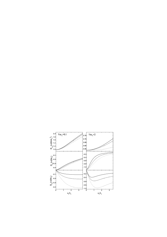
Figure 6: The calculated dependencies of the asymptotic diffusion coefficients on $\omega_{c}$. The solid, dashed, and dotted lines correspond to $\lambda_{y}/\lambda_{x}=0.5$, $1$, and $2$, respectively.

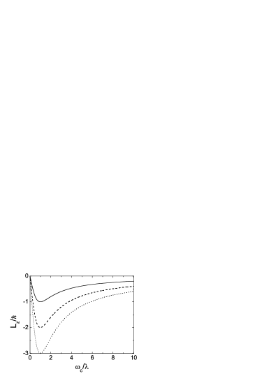
Figure 7: The calculated asymptotic $z$-component of angular momentum $L$ as a function of $\omega_{c}/\lambda$ at $\lambda_{x}=\lambda_{y}=\lambda$ and $\gamma/\lambda=12$. The solid, dashed, and dotted lines correspond to the cases with $T/(\hbar\lambda)=1$, $2$, and $3$, respectively.

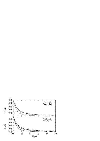
Figure 8: The calculated asymptotic $z$-component of angular momentum $L$ as a function of $\omega_{c}/\lambda$ at $T=0$. In upper part, $\gamma/\lambda=12$, $\lambda=\lambda_{x}$, $\lambda_{y}=\lambda_{x}=$1 (solid line), 2 (dashed line), 3 (dotted line). In lower part, $\lambda_{y}=\lambda_{x}=\lambda$, $\gamma/\lambda=1$ (solid line), 5 (dashed line), 20 (dotted line), 40 (dash-dotted line).

Note that the friction and resistance are quite different values and the diagonal components of resistance tensor

$$\rho(\infty)\sim\begin{pmatrix}m_{x}\lambda_{x}&&&m_{x}\omega_{cx}\\ -m_{y}\omega_{cy}&&&m_{y}\lambda_{y}\end{pmatrix}$$

obtained in our model does not depend on magnetic field. Moreover, the friction does not depend on magnetic field in the Markovian limit, $\gamma\rightarrow\infty$. The friction coefficients have relatively small influence on the process in the system at almost all spectrum of the magnetic field except for very weak fields. Analyzing the dependence of the frequency of microscopic magnetic field $\tilde{\omega}_{c}$ on $\lambda$, one can conclude that the specimen with nonzero friction perceives the external magnetic field with higher intensity. The non-Markovian corrections to the external magnetic field are larger for the system with longer time $\gamma^{-1}$ of response.

The dependencies of asymptotic variances and diffusion coefficients on magnetic field are shown in Figs. 5 and 6. At low temperature, the absolute values of $\Sigma_{\pi_{x}\pi_{x}}$ and $\Sigma_{x\pi_{y}}$ increase with the field while $\Sigma_{x\pi_{x}}$ shows the opposite trend. At high temperature, we have the same behavior for $\Sigma_{\pi_{x}\pi_{x}}$ and $\Sigma_{x\pi_{x}}$, but different dependence for $\Sigma_{x\pi_{y}}$. Its absolute value firstly increases with $\omega_{c}$, reaches the minimum, and then decreases. As seen, at low temperature, the increase of $\lambda_{y}$ with respect to $\lambda_{x}$ leads to larger absolute values of $\Sigma_{x\pi_{x}}$ ($D_{x\pi_{x}}$) and $\Sigma_{x\pi_{y}}$ ($D_{x\pi_{y}}$), and to smaller values of $\Sigma_{\pi_{x}\pi_{x}}$ ($D_{\pi_{x}\pi_{x}}$). With increasing temperature, $\Sigma_{x\pi_{x}}$ ($D_{x\pi_{x}}$) and $\Sigma_{\pi_{x}\pi_{x}}$ ($D_{\pi_{x}\pi_{x}}$) keep their behavior unchanged.

III.2 Orbital angular momentum component

We calculate the $z$-component of the angular momentum $L_{z}$ for the system settled in the increasing external magnetic field at different temperatures (Figs. 7 and 8). The results indicate the diamagnetism of the system even in the presence of a physical heat bath. As seen in Fig. 7, the absolute value of the magnetization of electric charges increases with temperature. At high $B$, the value of $L_{z}$ or $M$ tends to 0 as $\omega_{c}^{-1}$. At low temperatures and large $\gamma$, the value of $L_{z}$ approaches $\hbar$ with increasing $B$ ( Fig. 8). At $T\to 0$, $B\to\infty$, and $\gamma\to\infty$, we obtain the usual quantization of $L_{z}$ in the dissipative system.

IV Summary

The behavior of the generated flow of free charge carriers under the influence of external magnetic field was studied within the non-Markovian two-dimensional Langevin approach and the linear coupling in coordinate between the charge carriers and environment. In order to average the influence of bosonic heat-bath on the charged particle, we applied the spectral function of heat-bath excitations which describes the Drude dissipation with Lorenzian cutoffs. The analytical expressions for the time-dependent and asymptotic friction and diffusion coefficients, variances of the coordinates, cyclotron frequencies, orbital magnetic moment were obtained. The influence of an external magnetic field on the transport properties of an open quantum system was studied at the limits of low and high temperatures. Based on the calculations, one can conclude that the system in dissipative environment perceives the external magnetic field with higher intensity. The non-Markovian corrections to the external magnetic field are larger for the system with longer memory time. The decrease of asymptotic friction coefficients and the localization of the charged particle with increasing magnetic field were observed for the bosonic system. We demonstrated the survival of diamagnetism of the system in the presence of the realistic heat bath at low and high temperature regimes. For the orbital magnetic moment or angular momentum in the dissipative system, we obtained the quantization condition at $T\to 0$, $B\to\infty$, and $\gamma\to\infty$.

Appendix A Coefficients $J_{q_{i}q_{j}}(t)$

The explicit expressions for the coefficients

$$J_{xx}(t) = \ll I_{x}(t)I_{x}(t)+I^{\prime}_{x}(t)I^{\prime}_{x}(t)\gg,\hskip 7.22743ptJ_{yy}(t)=J_{xx}(t)|_{x\to y},$$

$$J_{xy}(t) = \ll I_{x}(t)I_{y}(t)+I^{\prime}_{x}(t)I^{\prime}_{y}(t)\gg,\hskip 7.22743ptJ_{\pi_{x}\pi_{y}}(t)=J_{xy}(t)|_{x\to\pi_{x},y\to\pi_{y}},$$

$$J_{x\pi_{x}}(t) = \ll I_{x}(t)I_{\pi_{x}}(t)+I^{\prime}_{x}(t)I^{\prime}_{\pi_{x}}(t)\gg,\hskip 7.22743ptJ_{y\pi_{x}}(t)|=J_{x\pi_{x}}(t)|_{x\to y},$$

$$J_{x\pi_{y}}(t) = \ll I_{x}(t)I_{\pi_{y}}(t)+I^{\prime}_{x}(t)I^{\prime}_{\pi_{y}}(t)\gg,\hskip 7.22743ptJ_{y\pi_{y}}(t)=J_{x\pi_{y}}(t)|_{x\to y},$$

$$J_{\pi_{x}\pi_{x}}(t) = \ll I_{\pi_{x}}(t)I_{\pi_{x}}(t)+I^{\prime}_{\pi_{x}}(t)I^{\prime}_{\pi_{x}}(t)\gg,\hskip 7.22743ptJ_{\pi_{y}\pi_{y}}(t)=J_{\pi_{x}\pi_{x}}(t)|_{pi_{x}\to\pi_{y}}.$$ (36)

are:

$$J_{xx}(t) = \frac{m\hbar\gamma^{2}}{\pi}\int_{0}^{\infty}d\omega\int_{0}^{t}dt^{\prime}\int_{0}^{t}dt^{\prime\prime}\frac{\omega\coth\left[\frac{\hbar\omega}{2T}\right]}{\omega^{2}+\gamma^{2}}$$

$$\times \left[\lambda_{x}A_{1}(t^{\prime})A_{1}(t^{\prime\prime})+\lambda_{y}A_{2}(t^{\prime})A_{2}(t^{\prime\prime})\right]\cos(\omega[t^{\prime\prime}-t^{\prime}]),$$

$$J_{yy}(t) = \frac{m\hbar\gamma^{2}}{\pi}\int_{0}^{\infty}d\omega\int_{0}^{t}dt^{\prime}\int_{0}^{t}dt^{\prime\prime}\frac{\omega\coth\left[\frac{\hbar\omega}{2T}\right]}{\omega^{2}+\gamma^{2}}$$

$$\times \left[\lambda_{x}B_{2}(t^{\prime})B_{2}(t^{\prime\prime})+\lambda_{y}B_{1}(t^{\prime})B_{1}(t^{\prime\prime})\right]\cos(\omega[t^{\prime\prime}-t^{\prime}]),$$

$$J_{xy}(t) = \frac{m\hbar\gamma^{2}}{\pi}\int_{0}^{\infty}d\omega\int_{0}^{t}dt^{\prime}\int_{0}^{t}dt^{\prime\prime}\frac{\omega\coth\left[\frac{\hbar\omega}{2T}\right]}{\omega^{2}+\gamma^{2}}$$

$$\times \left[\lambda_{x}A_{1}(t^{\prime})B_{2}(t^{\prime\prime})+\lambda_{y}A_{2}(t^{\prime})B_{1}(t^{\prime\prime})\right]\cos(\omega[t^{\prime\prime}-t^{\prime}]),$$

$$J_{\pi_{x}\pi_{x}}(t) = \frac{m\hbar\gamma^{2}}{\pi}\int_{0}^{\infty}d\omega\int_{0}^{t}dt^{\prime}\int_{0}^{t}dt^{\prime\prime}\frac{\omega\coth\left[\frac{\hbar\omega}{2T}\right]}{\omega^{2}+\gamma^{2}}$$

$$\times \left[\lambda_{x}C_{1}(t^{\prime})C_{1}(t^{\prime\prime})+\lambda_{y}C_{2}(t^{\prime})C_{2}(t^{\prime\prime})\right]\cos(\omega[t^{\prime\prime}-t^{\prime}]),$$

$$J_{\pi_{y}\pi_{y}}(t) = \frac{m\hbar\gamma^{2}}{\pi}\int_{0}^{\infty}d\omega\int_{0}^{t}dt^{\prime}\int_{0}^{t}dt^{\prime\prime}\frac{\omega\coth\left[\frac{\hbar\omega}{2T}\right]}{\omega^{2}+\gamma^{2}}$$

$$\times \left[\lambda_{x}D_{2}(t^{\prime})D_{2}(t^{\prime\prime})+\lambda_{y}D_{1}(t^{\prime})D_{1}(t^{\prime\prime})\right]\cos(\omega[t^{\prime\prime}-t^{\prime}]),$$

$$J_{\pi_{x}\pi_{y}}(t) = \frac{m\hbar\gamma^{2}}{\pi}\int_{0}^{\infty}d\omega\int_{0}^{t}dt^{\prime}\int_{0}^{t}dt^{\prime\prime}\frac{\omega\coth\left[\frac{\hbar\omega}{2T}\right]}{\omega^{2}+\gamma^{2}}$$

$$\times \left[\lambda_{x}C_{1}(t^{\prime})D_{2}(t^{\prime\prime})+\lambda_{y}C_{2}(t^{\prime})D_{1}(t^{\prime\prime})\right]\cos(\omega[t^{\prime\prime}-t^{\prime}]),$$

$$J_{x\pi_{x}}(t) = \frac{m\hbar\gamma^{2}}{\pi}\int_{0}^{\infty}d\omega\int_{0}^{t}dt^{\prime}\int_{0}^{t}dt^{\prime\prime}\frac{\omega\coth\left[\frac{\hbar\omega}{2T}\right]}{\omega^{2}+\gamma^{2}}$$

$$\times \left[\lambda_{x}A_{1}(t^{\prime})C_{1}(t^{\prime\prime})+\lambda_{y}A_{2}(t^{\prime})C_{2}(t^{\prime\prime})\right]\cos(\omega[t^{\prime\prime}-t^{\prime}]),$$

$$J_{y\pi_{y}}(t) = \frac{m\hbar\gamma^{2}}{\pi}\int_{0}^{\infty}d\omega\int_{0}^{t}dt^{\prime}\int_{0}^{t}dt^{\prime\prime}\frac{\omega\coth\left[\frac{\hbar\omega}{2T}\right]}{\omega^{2}+\gamma^{2}}$$

$$\times \left[\lambda_{x}B_{2}(t^{\prime})D_{2}(t^{\prime\prime})+\lambda_{y}B_{1}(t^{\prime})D_{1}(t^{\prime\prime})\right]\cos(\omega[t^{\prime\prime}-t^{\prime}]),$$

$$J_{x\pi_{y}}(t) = \frac{m\hbar\gamma^{2}}{\pi}\int_{0}^{\infty}d\omega\int_{0}^{t}dt^{\prime}\int_{0}^{t}dt^{\prime\prime}\frac{\omega\coth\left[\frac{\hbar\omega}{2T}\right]}{\omega^{2}+\gamma^{2}}$$

$$\times \left[\lambda_{x}A_{1}(t^{\prime})D_{2}(t^{\prime\prime})+\lambda_{y}A_{2}(t^{\prime})D_{1}(t^{\prime\prime})\right]\cos(\omega[t^{\prime\prime}-t^{\prime}]),$$

$$J_{y\pi_{x}}(t) = \frac{m\hbar\gamma^{2}}{\pi}\int_{0}^{\infty}d\omega\int_{0}^{t}dt^{\prime}\int_{0}^{t}dt^{\prime\prime}\frac{\omega\coth\left[\frac{\hbar\omega}{2T}\right]}{\omega^{2}+\gamma^{2}}$$

$$\times \left[\lambda_{x}B_{2}(t^{\prime})C_{1}(t^{\prime\prime})+\lambda_{y}B_{1}(t^{\prime})C_{2}(t^{\prime\prime})\right]\cos(\omega[t^{\prime\prime}-t^{\prime}]).$$

Appendix B Asymptotic variances at high and low temperature limits

At high temperature limit, the asymptotic variances are

$$\Sigma_{\pi_{x}\pi_{y}}(\infty)=0,$$

$${}\Sigma_{\pi_{x}\pi_{x}}(\infty)=m_{x}T,\hskip 14.45377pt\Sigma_{x\pi_{x}}(\infty)=\frac{\lambda_{y}T}{\lambda_{x}\lambda_{y}+\omega_{c}^{2}},\hskip 14.45377pt\Sigma_{x\pi_{y}}(\infty)=-\frac{\omega_{cx}T}{\lambda_{x}\lambda_{y}+\omega_{c}^{2}},$$

$${}\Sigma_{\pi_{y}\pi_{y}}(\infty)=\Sigma_{\pi_{x}\pi_{x}}(\infty)|_{x\leftrightarrow y},\hskip 3.61371pt\Sigma_{y\pi_{y}}(\infty)=\Sigma_{x\pi_{x}}(\infty)|_{x\leftrightarrow y},\hskip 3.61371pt\Sigma_{y\pi_{x}}(\infty)=-\Sigma_{x\pi_{y}}(\infty)|_{x\leftrightarrow y}.$$ (37)

At low temperature limit, we have

$$\Sigma_{\pi_{x}\pi_{y}}(\infty) = 0,$$

$$\Sigma_{\pi_{x}\pi_{x}}(\infty) = \frac{\hbar\gamma^{2}m}{\pi\delta}\{\lambda_{y}\gamma^{2}\varpi_{1}(\lambda_{x}\lambda_{y}+\omega_{c}^{2})+\varpi_{2}(\lambda_{x}\gamma[\gamma-2\lambda_{y}]+\lambda_{y}\omega_{c}^{2})+\varpi_{3}\lambda_{x}\},$$

$$\Sigma_{x\pi_{x}}(\infty) = \frac{\hbar\gamma^{2}}{\pi(\lambda_{x}\lambda_{y}+\omega_{c}^{2})\Delta}\{\gamma^{3}\lambda_{y}^{2}\zeta_{1}(\lambda_{x}-\gamma)(\lambda_{x}\lambda_{y}+\omega_{c}^{2})$$

$$- \gamma\lambda_{y}\zeta_{2}(\gamma\lambda_{x}[\lambda_{y}(\lambda_{y}+2\lambda_{x})-\gamma(2\lambda_{y}+\lambda_{x})+\gamma^{2}]+\omega_{c}^{2}[\lambda_{y}\lambda_{x}+\gamma(\lambda_{y}-\lambda_{x})])$$

$$+ \lambda_{x}\lambda_{y}\zeta_{3}([\lambda_{x}+2(\lambda_{y}-\gamma)]\gamma+\omega_{c}^{2})-\lambda_{x}\zeta_{4}\lambda_{y}\},$$

$$\Sigma_{x\pi_{y}}(\infty) = -\frac{\hbar\gamma^{2}\omega_{c}}{\pi(\lambda_{x}\lambda_{y}+\omega_{c}^{2})\Delta}\{\gamma^{3}\lambda_{x}\zeta_{1}(\gamma-\lambda_{y})(\lambda_{x}\lambda_{y}+\omega_{c}^{2})$$

$$+ \gamma\zeta_{2}(\omega_{c}^{2}\lambda_{x}[2\gamma+\lambda_{y}]-\lambda_{y}[2\lambda_{x}(\lambda_{x}\lambda_{y}+\omega_{c}^{2})-\lambda_{x}\gamma(3\lambda_{y}+2[\lambda_{x}-\gamma])-\gamma^{2}(\gamma-\lambda_{y})])$$

$$+ \zeta_{3}(\lambda_{x}\omega_{c}^{2}+\lambda_{y}[\lambda_{x}(\lambda_{x}+\lambda_{y})+2\gamma(\gamma-\lambda_{x})-\lambda_{y}\gamma])+\zeta_{4}\lambda_{y}\},$$

$$\Sigma_{\pi_{y}\pi_{y}}(\infty) = \Sigma_{\pi_{x}\pi_{x}}(\infty)|_{x\leftrightarrow y},\hskip 3.61371pt\Sigma_{y\pi_{y}}(\infty)=\Sigma_{x\pi_{x}}(\infty)|_{x\leftrightarrow y},\hskip 3.61371pt\Sigma_{y\pi_{x}}(\infty)=-\Sigma_{x\pi_{y}}(\infty)|_{x\leftrightarrow y},$$ (38)

where

$$\delta = (s_{1}^{2}-s_{2}^{2})(s_{1}^{2}-s_{3}^{2})(s_{1}^{2}-s_{4}^{2})(s_{2}^{2}-s_{3}^{2})(s_{2}^{2}-s_{4}^{2})(s_{3}^{2}-s_{4}^{2}),$$

$$\Delta = (\gamma^{2}-s_{1}^{2})(\gamma^{2}-s_{2}^{2})(\gamma^{2}-s_{3}^{2})(\gamma^{2}-s_{4}^{2})\delta,$$ (39)

and

$$\varpi_{1} = (s_{1}s_{2})^{4}(s_{1}^{2}-s_{2}^{2})\ln\left[\frac{s_{1}}{s_{2}}\right]+(s_{1}s_{3})^{4}(s_{3}^{2}-s_{1}^{2})\ln\left[\frac{s_{3}}{s_{1}}\right]+(s_{1}s_{4})^{4}(s_{1}^{2}-s_{4}^{2})\ln\left[\frac{s_{1}}{s_{4}}\right]$$

$$+ (s_{2}s_{3})^{4}(s_{2}^{2}-s_{3}^{2})\ln\left[\frac{s_{2}}{s_{3}}\right]+(s_{2}s_{4})^{4}(s_{4}^{2}-s_{2}^{2})\ln\left[\frac{s_{4}}{s_{2}}\right]+(s_{3}s_{4})^{4}(s_{3}^{2}-s_{4}^{2})\ln\left[\frac{s_{3}}{s_{4}}\right],$$

$$\varpi_{2} = (s_{1}s_{2})^{2}(s_{3}^{4}-s_{4}^{4})\ln\left[\frac{s_{1}}{s_{2}}\right]+(s_{1}s_{3})^{2}(s_{4}^{4}-s_{2}^{4})\ln\left[\frac{s_{1}}{s_{3}}\right]+(s_{1}s_{4})^{2}(s_{4}^{2}-s_{3}^{4})\ln\left[\frac{s_{1}}{s_{4}}\right]$$

$$+ (s_{2}s_{3})^{2}(s_{1}^{4}-s_{4}^{4})\ln\left[\frac{s_{2}}{s_{3}}\right]+(s_{2}s_{4})^{2}(s_{3}^{4}-s_{1}^{4})\ln\left[\frac{s_{2}}{s_{4}}\right]+(s_{3}s_{4})^{2}(s_{1}^{4}-s_{2}^{4})\ln\left[\frac{s_{3}}{s_{4}}\right],$$

$$\varpi_{3} = (s_{1}s_{2})^{4}(s_{3}^{2}-s_{4}^{2})\ln\left[\frac{s_{1}}{s_{2}}\right]+(s_{1}s_{3})^{4}(s_{4}^{2}-s_{2}^{2})\ln\left[\frac{s_{1}}{s_{3}}\right]+(s_{1}s_{4})^{4}(s_{2}^{2}-s_{3}^{2})\ln\left[\frac{s_{1}}{s_{4}}\right]$$

$$+ (s_{2}s_{3})^{4}(s_{1}^{2}-s_{4}^{2})\ln\left[\frac{s_{2}}{s_{3}}\right]+(s_{2}s_{4})^{4}(s_{3}^{2}-s_{1}^{2})\ln\left[\frac{s_{2}}{s_{4}}\right]+(s_{3}s_{4})^{4}(s_{1}^{2}-s_{2}^{2})\ln\left[\frac{s_{3}}{s_{4}}\right],$$

$$\zeta_{1}=(s_{2}s_{3}s_{4})^{2}(s_{2}^{2}-s_{3}^{2})(s_{2}^{2}-s_{4}^{2})(s_{3}^{2}-s_{4}^{2})\ln\left[\frac{\gamma}{s_{1}}\right]$$

$${}+(s_{1}s_{3}s_{4})^{2}(s_{1}^{2}-s_{3}^{2})(s_{1}^{2}-s_{4}^{2})(s_{3}^{2}-s_{4}^{2})\ln\left[\frac{\gamma}{s_{2}}\right]$$

$${}+(s_{1}s_{2}s_{4})^{2}(s_{1}^{2}-s_{2}^{2})(s_{2}^{2}-s_{4}^{2})(s_{1}^{2}-s_{4}^{2})\ln\left[\frac{\gamma}{s_{3}}\right]$$

$${}+(s_{1}s_{2}s_{3})^{2}(s_{2}^{2}-s_{3}^{2})(s_{1}^{2}-s_{2}^{2})(s_{1}^{2}-s_{3}^{2})\ln\left[\frac{\gamma}{s_{4}}\right]$$

$${}+(\gamma s_{3}s_{4})^{2}(\gamma^{2}-s_{3}^{2})(\gamma^{2}-s_{4}^{2})(s_{3}^{2}-s_{4}^{2})\ln\left[\frac{s_{1}}{s_{2}}\right]$$

$${}+(\gamma s_{2}s_{4})^{2}(\gamma^{2}-s_{2}^{2})(\gamma^{2}-s_{4}^{2})(s_{2}^{2}-s_{4}^{2})\ln\left[\frac{s_{1}}{s_{3}}\right]$$

$${}+(\gamma s_{2}s_{3})^{2}(\gamma^{2}-s_{2}^{2})(\gamma^{2}-s_{3}^{2})(s_{2}^{2}-s_{3}^{2})\ln\left[\frac{s_{1}}{s_{4}}\right]$$

$${}+(\gamma s_{1}s_{4})^{2}(\gamma^{2}-s_{1}^{2})(\gamma^{2}-s_{4}^{2})(s_{1}^{2}-s_{4}^{2})\ln\left[\frac{s_{2}}{s_{3}}\right]$$

$${}+(\gamma s_{1}s_{3})^{2}(\gamma^{2}-s_{1}^{2})(\gamma^{2}-s_{3}^{2})(s_{1}^{2}-s_{3}^{2})\ln\left[\frac{s_{2}}{s_{4}}\right]$$

$${}+(\gamma s_{1}s_{2})^{2}(\gamma^{2}-s_{1}^{2})(\gamma^{2}-s_{2}^{2})(s_{1}^{2}-s_{2}^{2})\ln\left[\frac{s_{3}}{s_{4}}\right],$$

$$\zeta_{2} = (\gamma s_{1})^{2}[(s_{2}s_{3})^{2}+(s_{2}s_{4})^{2}+(s_{3}s_{4})^{2}](s_{2}^{2}-s_{3}^{2})(s_{2}^{2}-s_{4}^{2})(s_{3}^{2}-s_{4}^{2})\ln\left[\frac{\gamma}{s_{1}}\right]$$

$$+ (\gamma s_{2})^{2}[(s_{1}s_{3})^{2}+(s_{1}s_{4})^{2}+(s_{3}s_{4})^{2}](s_{1}^{2}-s_{3}^{2})(s_{1}^{2}-s_{4}^{2})(s_{3}^{2}-s_{4}^{2})\ln\left[\frac{\gamma}{s_{2}}\right]$$

$$+ (\gamma s_{3})^{2}[(s_{1}s_{2})^{2}+(s_{1}s_{4})^{2}+(s_{2}s_{4})^{2}](s_{1}^{2}-s_{2}^{2})(s_{2}^{2}-s_{4}^{2})(s_{1}^{2}-s_{4}^{2})\ln\left[\frac{\gamma}{s_{3}}\right]$$

$$+ (\gamma s_{4})^{2}[(s_{1}s_{2})^{2}+(s_{1}s_{3})^{2}+(s_{2}s_{3})^{2}](s_{2}^{2}-s_{3}^{2})(s_{1}^{2}-s_{2}^{2})(s_{1}^{2}-s_{3}^{2})\ln\left[\frac{\gamma}{s_{4}}\right]$$

$$+ (s_{1}s_{2})^{2}[(\gamma s_{3})^{2}+(\gamma s_{4})^{2}+(s_{3}s_{4})^{2}](\gamma^{2}-s_{3}^{2})(\gamma^{2}-s_{4}^{2})(s_{3}^{2}-s_{4}^{2})\ln\left[\frac{s_{1}}{s_{2}}\right]$$

$$+ (s_{1}s_{3})^{2}[(\gamma s_{2})^{2}+(\gamma s_{4})^{2}+(s_{2}s_{4})^{2}](\gamma^{2}-s_{2}^{2})(\gamma^{2}-s_{4}^{2})(s_{2}^{2}-s_{4}^{2})\ln\left[\frac{s_{1}}{s_{3}}\right]$$

$$+ (s_{1}s_{4})^{2}[(\gamma s_{2})^{2}+(\gamma s_{3})^{2}+(s_{2}s_{3})^{2}](\gamma^{2}-s_{2}^{2})(\gamma^{2}-s_{3}^{2})(s_{2}^{2}-s_{3}^{2})\ln\left[\frac{s_{1}}{s_{4}}\right]$$

$$+ (s_{2}s_{3})^{2}[(\gamma s_{1})^{2}+(\gamma s_{4})^{2}+(s_{1}s_{4})^{2}](\gamma^{2}-s_{1}^{2})(\gamma^{2}-s_{4}^{2})(s_{1}^{2}-s_{4}^{2})\ln\left[\frac{s_{2}}{s_{3}}\right]$$

$$+ (s_{2}s_{4})^{2}[(\gamma s_{1})^{2}+(s_{3})^{2}+(s_{1}s_{3})^{2}](\gamma^{2}-s_{1}^{2})(\gamma^{2}-s_{3}^{2})(s_{1}^{2}-s_{3}^{2})\ln\left[\frac{s_{2}}{s_{4}}\right]$$

$$+ (s_{3}s_{4})^{2}[(\gamma s_{1})^{2}+(\gamma s_{2})^{2}+(s_{1}s_{2})^{2}](\gamma^{2}-s_{1}^{2})(\gamma^{2}-s_{2}^{2})(s_{1}^{2}-s_{2}^{2})\ln\left[\frac{s_{3}}{s_{4}}\right],$$

$$\zeta_{3} = (\gamma s_{1})^{4}(s_{2}^{2}+s_{3}^{2}+s_{4}^{2})(s_{2}^{2}-s_{3}^{2})(s_{2}^{2}-s_{4}^{2})(s_{3}^{2}-s_{4}^{2})\ln\left[\frac{\gamma}{s_{1}}\right]$$

$$+ (\gamma s_{2})^{4}(s_{1}^{2}+s_{3}^{2}+s_{4}^{2})(s_{1}^{2}-s_{3}^{2})(s_{1}^{2}-s_{4}^{2})(s_{3}^{2}-s_{4}^{2})\ln\left[\frac{\gamma}{s_{2}}\right]$$

$$+ (\gamma s_{3})^{4}(s_{1}^{2}+s_{2}^{2}+s_{4}^{2})(s_{1}^{2}-s_{2}^{2})(s_{2}^{2}-s_{4}^{2})(s_{1}^{2}-s_{4}^{2})\ln\left[\frac{\gamma}{s_{3}}\right]$$

$$+ (\gamma s_{4})^{4}(s_{1}^{2}+s_{2}^{2}+s_{3}^{2})(s_{2}^{2}-s_{3}^{2})(s_{1}^{2}-s_{2}^{2})(s_{1}^{2}-s_{3}^{2})\ln\left[\frac{\gamma}{s_{4}}\right]$$

$$+ (s_{1}s_{2})^{4}(\gamma^{2}+s_{3}^{2}+s_{4}^{2})(\gamma^{2}-s_{3}^{2})(\gamma^{2}-s_{4}^{2})(s_{3}^{2}-s_{4}^{2})\ln\left[\frac{s_{1}}{s_{2}}\right]$$

$$+ (s_{1}s_{3})^{4}(\gamma^{2}+s_{2}^{2}+s_{4}^{2})(\gamma^{2}-s_{2}^{2})(\gamma^{2}-s_{4}^{2})(s_{2}^{2}-s_{4}^{2})\ln\left[\frac{s_{1}}{s_{3}}\right]$$

$$+ (s_{1}s_{4})^{4}(\gamma^{2}+s_{2}^{2}+s_{3}^{2})(\gamma^{2}-s_{2}^{2})(\gamma^{2}-s_{3}^{2})(s_{2}^{2}-s_{3}^{2})\ln\left[\frac{s_{1}}{s_{4}}\right]$$

$$+ (s_{2}s_{3})^{4}(\gamma^{2}+s_{1}^{2}+s_{4}^{2})(\gamma^{2}-s_{1}^{2})(\gamma^{2}-s_{4}^{2})(s_{1}^{2}-s_{4}^{2})\ln\left[\frac{s_{2}}{s_{3}}\right]$$

$$+ (s_{2}s_{4})^{4}(\gamma^{2}+s_{1}^{2}+s_{3}^{2})(\gamma^{2}-s_{1}^{2})(\gamma^{2}-s_{3}^{2})(s_{1}^{2}-s_{3}^{2})\ln\left[\frac{s_{2}}{s_{4}}\right]$$

$$+ (s_{3}s_{4})^{4}(\gamma^{2}+s_{1}^{2}+s_{2}^{2})(\gamma^{2}-s_{1}^{2})(\gamma^{2}-s_{2}^{2})(s_{1}^{2}-s_{2}^{2})\ln\left[\frac{s_{3}}{s_{4}}\right],$$

$$\zeta_{4}=(\gamma s_{1})^{6}(s_{2}^{2}-s_{3}^{2})(s_{2}^{2}-s_{4}^{2})(s_{3}^{2}-s_{4}^{2})\ln\left[\frac{\gamma}{s_{1}}\right]$$

$${}+(\gamma s_{2})^{6}(s_{1}^{2}-s_{3}^{2})(s_{1}^{2}-s_{4}^{2})(s_{3}^{2}-s_{4}^{2})\ln\left[\frac{\gamma}{s_{2}}\right]$$

$${}+(\gamma s_{3})^{6}(s_{1}^{2}-s_{2}^{2})(s_{2}^{2}-s_{4}^{2})(s_{1}^{2}-s_{4}^{2})\ln\left[\frac{\gamma}{s_{3}}\right]$$

$${}+(\gamma s_{4})^{6}(s_{2}^{2}-s_{3}^{2})(s_{1}^{2}-s_{2}^{2})(s_{1}^{2}-s_{3}^{2})\ln\left[\frac{\gamma}{s_{4}}\right]$$

$${}+(s_{1}s_{2})^{6}(\gamma^{2}-s_{3}^{2})(\gamma^{2}-s_{4}^{2})(s_{3}^{2}-s_{4}^{2})\ln\left[\frac{s_{1}}{s_{2}}\right]$$

$${}+(s_{1}s_{3})^{6}(\gamma^{2}-s_{2}^{2})(\gamma^{2}-s_{4}^{2})(s_{2}^{2}-s_{4}^{2})\ln\left[\frac{s_{1}}{s_{3}}\right]$$

$${}+(s_{1}s_{4})^{6}(\gamma^{2}-s_{2}^{2})(\gamma^{2}-s_{3}^{2})(s_{2}^{2}-s_{3}^{2})\ln\left[\frac{s_{1}}{s_{4}}\right]$$

$${}+(s_{2}s_{3})^{6}(\gamma^{2}-s_{1}^{2})(\gamma^{2}-s_{4}^{2})(s_{1}^{2}-s_{4}^{2})\ln\left[\frac{s_{2}}{s_{3}}\right]$$

$${}+(s_{2}s_{4})^{6}(\gamma^{2}-s_{1}^{2})(\gamma^{2}-s_{3}^{2})(s_{1}^{2}-s_{3}^{2})\ln\left[\frac{s_{2}}{s_{4}}\right]$$

$${}+(s_{3}s_{4})^{6}(\gamma^{2}-s_{1}^{2})(\gamma^{2}-s_{2}^{2})(s_{1}^{2}-s_{2}^{2})\ln\left[\frac{s_{3}}{s_{4}}\right].$$