Dissipative and Hall viscosity of a disordered 2D electron gas

Abstract

Hydrodynamic charge transport is at the center of recent research efforts. Of particular interest is the nondissipative Hall viscosity, which conveys topological information in clean gapped systems. The prevalence of disorder in the real world calls for a study of its effect on viscosity. Here we address this question, both analytically and numerically, in the context of a disordered noninteracting 2D electrons. Analytically, we employ the self-consistent Born approximation, explicitly taking into account the modification of the single-particle density of states and the elastic transport time due to the Landau quantization. The reported results interpolate smoothly between the limiting cases of weak (strong) magnetic field and strong (weak) disorder. In the regime of weak magnetic field our results describes the quantum (Shubnikov-de Haas type) oscillations of the dissipative and Hall viscosity. For strong magnetic fields we characterize the effects of the disorder-induced broadening of the Landau levels on the viscosity coefficients. This is supplemented by numerical calculations for a few filled Landau levels. Our results show that the Hall viscosity is surprisingly robust to disorder.

Introduction. — Ordinary fluid motion is described by the theory of hydrodynamics, one of whose cornerstones is viscosity, which serves as the source of dissipation. Under certain conditions, charge transport in an electronic system can also be dominated by hydrodynamic viscous flow Gurzhi ; Molenkamp . The discovery of graphene stimulated renewed theoretical Muller2009 ; Andreev2011 ; Polini2015 ; Levitov2016 ; NGMS ; Levitov2017 ; Kashuba ; Lucas2018 ; Schmalian and experimental Titov2013 ; Polini2016 ; Kim2016 ; Moll2016 ; Geim2017 ; Levitov2018 ; Kvon2018 interest in the hydrodynamic description of charge conduction.

In the absence of time-reversal symmetry the viscosity tensor has non-dissipative antisymmetric components. In the presence of a magnetic field $B$, this non-dissipative Hall viscosity ($\eta_{H}$) was studied theoretically in the classical limit of high temperature plasmas CC ; Marshall ; Kaufman ; Thompson ; Braginskii , and for low temperature electron gas Steinberg . Later, interest in the Hall viscosity was rekindled in quantum systems with a gapped spectrum, due to the connection between $\eta_{H}$ and geometric response Avron ; Levay ; Avron1998 ; Read ; RR ; Haldane ; HLF , and its expected quantization in the presence of translational and rotational symmetries RR . It was understood that beyond the Hall conductivity and viscosity there are additional non-dissipative electro-magnetic and geometrical response functions in gapped quantum systems HS2012 ; Abanov2013 ; AG2014 ; GA2014 ; Hoyos ; Andreev ; Wiegmann2014 ; GA2015 ; Wiegmann2015 ; Gurarie ; Andreev2015 ; NG2017 ; NCG2017 . Within the hydrodynamic description of electron transport, non-zero $\eta_{H}$ influences significantly the structure of the electron flow Alekseev ; PTP ; SNSMM ; DG2017 ; GA2017 ; Alekseev-2 , which allows one to access $\eta_{H}$ experimentally Bandurin2018 . Also, it was argued that the dissipative and Hall viscosity affect the spectrum of edge magnetoplasmons ACG2018 ; SDVV ; CG .

For noninteracting electrons in the absence of disorder each filled Landau level (LL) gives a contribution to the Hall viscosity equal $\hbar(2n+1)/(8\pi l_{B}^{2})$ Avron , where $n$ denotes the LL index and $l_{B}=\sqrt{\hbar c/(eB)}$ stands for the magnetic length. This result is stable against perturbations of the Hamiltonian which preserve translational and rotational invariance RR . However, the fate of this result in the presence of disorder has not been studied yet. Therefore, it is not clear how the clean result obtained within the quantum treatment of the electron motion in a magnetic field connects to the result $\eta_{H}=\nu_{0}\mu^{2}\omega_{c}\tau_{{\rm tr},2}^{2}/[1+4\omega_{c}^{2}\tau_{{\rm tr},2}^{2}]$ derived for a classical disordered electron gas Steinberg . Here $\mu$ denotes the chemical potential, $\tau_{{\rm tr},2}$ the second transport time, $\omega_{c}=eB/(mc)$ the cyclotron frequency, $\nu_{0}=m/(2\pi\hbar^{2})$ the density of states at $B=0$, and $m$ the effective electron mass.

In this Letter we report the results of an analytical and numerical study of the dissipative and Hall viscosities of noninteracting 2D electrons in the presence of disorder. Contrary to previous studies we explicitly take into account the Landau quantization of the electron spectrum. Analytically, within the self-consistent Born approximation (SCBA) AFS we derive expressions for the dissipative and Hall viscosities, which smoothly interpolates between the results known in the literature for classical magnetic field CC ; Marshall ; Kaufman ; Thompson ; Braginskii ; Alekseev and for the strong magnetic field in the absence of disorder Avron . Since the SCBA is rigorously justified for high LLs only, we perform numerical calculation of $\eta_{H}$ for a few lowest LLs. The obtained numerical results are in a perfect agreement with the SCBA predictions. They demonstrate a surprising resilience of the Hall viscosity to disorder.

Model. — Noninteracting electrons confined to a 2D plane are described by the following Hamiltonian

$$H=\bigl{(}-i\nabla-e\bm{A}\bigr{)}^{2}/2m+V(\bm{r}),$$ (1)

where $V(\bm{r})$ stands for a random potential and $\bm{A}$ for the vector potential corresponding to the static perpendicular magnetic field $B$. In this paper we use the Landau gauge: $A_{y}=-Bx$ and $A_{x}=A_{z}=0$. We assume that the random potential has Gaussian distribution with a pair correlation function $\overline{V(\bm{r})V(\bm{r^{\prime}})}=W(|\bm{r}-\bm{r^{\prime}}|)$ which decays with a typical length scale $d$. In what follows we use units with $e=c=\hbar=k_{B}=1$.

Kubo formula for the viscosity. — The viscosity tensor can be computed by means of the Kubo formula Resibois ; McLennan ; Bradlyn2012 :

$$\eta_{jk,ps}(\omega)= -\frac{i\kappa^{-1}}{\omega}\delta_{jk}\delta_{ps}+\frac{1}{i\omega S}\int\frac{d\Omega d\varepsilon}{\pi^{2}}\frac{f_{\varepsilon}-f_{\varepsilon+\Omega}}{\Omega-\omega-i0}$$

$$\times\overline{\operatorname{Tr}T_{jk}\operatorname{Im}G^{R}_{\varepsilon+\Omega}T_{ps}\operatorname{Im}G^{R}_{\varepsilon}}.$$ (2)

Here $f_{\varepsilon}=1/[1+\exp((\varepsilon-\mu)/T)]$ denotes the Fermi distribution function, $G^{R}_{\varepsilon}=1/(\varepsilon-H-i0)$ the retarded Green’s function, $S$ the system area, and $\kappa$ the internal compressibility Footnote1 . The form of the stress tensor, $T_{jk}=m(v_{j}v_{k}+v_{k}v_{j})/2$ is not affected by a random potential (see Ref. Irving1950 and the Supplemental Material for details SM ). Here $\bm{v}=(-i\nabla-e\bm{A})/m$ stands for the velocity operator. Disorder averaging is denoted by an overbar.

Self-consistent Born approximation. — In order to compute the viscosity tensor from Eq. (2) we treat the disorder scattering using the SCBA AFS . This approximation holds under the following conditions RS ; LA :

$$1/k_{F},d\ll l_{B},\qquad d\ll v_{F}\tau_{0}.$$ (3)

Here $k_{F}=mv_{F}$ and $v_{F}$ denote the Fermi momentum and velocity, respectively, and $\tau_{0}$ is the total elastic relaxation time at zero magnetic field. It can be expressed in terms of the Fourier transform $\tilde{W}(\bm{q})$ of the pair correlation function $W(\bm{r})$. Furthermore, it is convenient to generalize it to ($m=0,1,2,\dots$):

$$\frac{1}{\tau_{m}}=\nu_{0}\int_{0}^{2\pi}d\phi\,\tilde{W}(2k_{F}\sin\phi/2)\cos m\phi.$$ (4)

The average density of states $\nu(\varepsilon)$ at non-zero $B$ is determined by the average retarded Green’s function $\mathcal{G}^{R}_{\varepsilon}$. In the LL representation the average density of states is given as $\nu(\varepsilon)=-\sum_{n}\operatorname{Im}\mathcal{G}^{R}_{n}(\varepsilon)/(2\pi^{2}l_{B}^{2})$. Within SCBA the retarded Green’s function satisfies AFS ; RS ; LA

$$\mathcal{G}^{R}_{n}=(\varepsilon-\epsilon_{n}-\Sigma^{R}_{\varepsilon})^{-1},\quad\Sigma^{R}_{\varepsilon}=\frac{\omega_{c}}{2\pi\tau_{0}}\sum_{n}\mathcal{G}^{R}_{n},$$ (5)

where $\epsilon_{n}=\omega_{c}(n+1/2)$. There are two limiting cases in which the self-consistent Eq. (5) can be easily solved AFS . In the regime of overlapping LLs, $\omega_{c}\tau_{0}\ll 1$, one can use the Poisson formula for summation over LL index. The averaged density of states becomes $\nu(\varepsilon)=\nu_{0}[1-2\delta\cos(2\pi\varepsilon/\omega_{c})]$. Here $\delta=\exp(-\pi/\omega_{c}\tau_{0})\ll 1$ is the Dingle parameter. In the opposite case, when the LLs are well separated, one can restrict the summation in Eq. (5) to the single LL which is closest to the energy of interest, $|\varepsilon-\epsilon_{N}|<\omega_{c}/2$. Then the average density of states acquires the semi-circle profile: $\nu(\varepsilon)=\nu_{0}\tau_{0}\sqrt{\Gamma^{2}-(\varepsilon-\epsilon_{N})^{2}}$, where $\Gamma=\sqrt{2\omega_{c}/(\pi\tau_{0})}$ determines the the broadened LL width.

In the presence of long-range disorder correlations, $d\gg k_{F}^{-1}$, it is important to take into account the vertex corrections to the “bubble” contribution in the Kubo formula (2) (see Fig. 1). This implies that in addition to the average Green’s function, one also needs to know the renormalized vertex, which is the stress tensor in the case of the viscosity. Within the SCBA $T_{jk}$ can be approximated as a linear combination of operators which change the LL index by $2$. Under conditions (3) one can show that an operator $V_{m}$, which transfers an electron from the $(n+m)$-th LL to the $n$-th LL, is renormalized by the ladder resummation of the disorder lines as follows RS ; LA ; DMP (see SM for details):

$$V_{m}\to\frac{V_{m}}{1-\tau_{m}^{-1}\Pi_{m}^{RA}},\,\Pi_{m}^{RA}=\frac{\omega_{c}}{2\pi}\sum_{n}\mathcal{G}^{R}_{n+m}(\varepsilon)\mathcal{G}^{A}_{n}(\varepsilon).$$ (6)

Here $\Pi_{m}^{RA}$ is the contribution of the bubble without ladder insertions. Using Eq. (5), it can be rewritten as $\Pi_{m}^{RA}=\color[rgb]{0,0,0}-\color[rgb]{0,0,0}i\nu(\varepsilon)/[m\omega_{c}\nu_{0}-i\nu(\varepsilon)\color[rgb]{0,0,0}/\tau_{0}\color[rgb]{0,0,0}]$. Therefore, within the SCBA the vertex corrections are expressed in terms of the average density of states only.

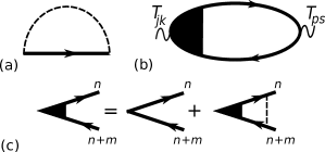
Figure 1: (a) The self-energy diagram. (b) The diagram corresponding to the Kubo formula (2). (c) The equation for the vertex $V_{m}$ in the ladder approximation. The solid line denotes the SCBA Green’s function $\mathcal{G}(\varepsilon)$. The dashed line denotes the disorder correlation function $W(\bm{r})$.

Dissipative viscosity. — Disorder averaging restores 2D rotational symmetry note:rotation . Hence, the viscosity tensor $\eta_{jk,ps}$ is characterized by only three parameters:

$$\eta_{jk,ps} =\eta_{s}\bigl{(}\delta_{jp}\delta_{ks}+\delta_{js}\delta_{kp}\bigr{)}+\bigl{(}\zeta-\eta_{s}\bigr{)}\delta_{jk}\delta_{ps}$$

$$+(\eta_{H}/2)\bigl{(}\epsilon_{jp}\delta_{ks}+\epsilon_{js}\delta_{kp}+\epsilon_{kp}\delta_{js}+\epsilon_{ks}\delta_{jp}\bigr{)},$$ (7)

where $\zeta$ and $\eta_{s}$ denotes the bulk and shear viscosities, respectively. Within the SCBA the bulk viscosity vanishes, $\zeta=0$. Using Eqs. (5) and (6), we find the following result for the shear viscosity at $\omega=0$ SM :

$$\eta_{s}=\frac{1}{2}\int d\varepsilon\bigl{(}-f^{\prime}_{\varepsilon}\bigr{)}\frac{\nu(\varepsilon)\varepsilon^{2}\tau_{\rm tr,2}(\varepsilon)}{1+4\omega_{c}^{2}\tau_{\rm tr,2}^{2}(\varepsilon)},$$ (8)

where $\tau_{\rm tr,2}(\varepsilon)=\tau_{\rm tr,2}\nu_{0}/\nu(\varepsilon)$ is the renormalized second transport time and $1/\tau_{\rm tr,2}=1/\tau_{0}-1/\tau_{2}$ is the second transport rate at $B=0$. We note that for $k_{F}d\gg 1$ the second transport time becomes $\tau_{\rm tr,2}=\tau_{0}(k_{F}d/2)^{2}\gg\tau_{0}$. We mention that Eq. (8) is analogous to the result for the dissipative conductivity DMP .

In the regime of overlapping LLs, $\omega_{c}\tau_{0}\ll 1$, the shear viscosity exhibits Shubnikov-de Haas-type oscillations:

$$\eta_{s}=\frac{1}{2}\frac{\nu_{0}\mu^{2}\tau_{\rm tr,2}}{1+4\alpha^{2}}\left(1-\frac{16\alpha^{2}\delta}{1+4\alpha^{2}}\mathcal{F}_{T}\cos\frac{2\pi\mu}{\omega_{c}}\right),$$ (9)

where $\alpha=\omega_{c}\tau_{\rm tr,2}$ and $\mathcal{F}_{T}=(2\pi^{2}T/\omega_{c})/\sinh(2\pi^{2}T/\omega_{c})$. The non-oscillatory term in $\eta_{s}$ reproduces the classical result for the shear viscosity of an electron gas Steinberg .

In the regime of well separated LLs, $\omega_{c}\tau_{0}\gg 1$, one finds from Eq. (8) that the shear viscosity is non-zero when the chemical potential is inside the $N$-th broadened Landau level ($|\mu-\epsilon_{N}|\leqslant\Gamma$):

$$\eta_{s}=(N^{2}\tau_{0})/(8\pi^{2}l_{B}^{2}\tau_{\rm tr,2})\bigl{[}1-(\mu-\epsilon_{N})^{2}/\Gamma^{2}\bigr{]}.$$ (10)

For chemical potential at the center of the LL, the shear viscosity is $2\omega_{c}\tau_{0}/\pi$ times larger when one naively expects on the basis of purely classical expression. The dependence of the shear viscosity on the chemical potential in comparison with $\nu(\varepsilon)$ is shown in Fig.  2.

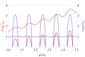
Figure 2: The density of states (blue dotted and blue dash-dotted curves) and shear viscosity (red solid and red dashed curves) as functions of $\mu/\omega_{c}$ for smooth disorder, $\tau_{\rm tr,2}/\tau_{0}=40$. Blue dotted and red solid curves correspond to well-separated LLs with $\omega_{c}\tau_{0}=15$. Blue dash-dotted and red dashed curves correspond to overlapping LLs with $\omega_{c}\tau_{0}=0.8$.

Hall viscosity. — The Hall viscosity can be extracted from the viscosity tensor as $\eta_{H}=(\eta_{xy,xx}-\eta_{xy,yy})/2$. Similarly to the Hall conductance, the evaluation of $\eta_{H}$ from the Kubo formula (2) is complicated due to contributions which come from all the states below the chemical potential. Therefore, it is convenient to proceed in a way pioneered by Smrčka and Středa SmSt : As for the Hall conductivity we split the expression for the Hall viscosity at $\omega=0$ into two parts, $\eta_{H}=\eta_{H}^{I}+\eta_{H}^{II}$, where SM

$$\eta_{H}^{I}= \operatorname{Re}\int\frac{d\varepsilon}{4\pi S}\bigl{(}-f^{\prime}_{\varepsilon}\bigr{)}\overline{\operatorname{Tr}T_{xy}G^{R}_{\varepsilon}\bigl{(}T_{xx}-T_{yy}\bigr{)}G^{A}_{\varepsilon}},$$ (11)

$$\eta_{H}^{II}= \operatorname{Im}\int\frac{d\varepsilon}{2\pi S}\bigl{(}-f^{\prime}_{\varepsilon}\bigr{)}\overline{\operatorname{Tr}J_{xy}(T_{yy}-T_{xx})G^{A}_{\varepsilon}}$$

$$+\operatorname{Im}\int\frac{d\varepsilon}{2\pi S}f_{\varepsilon}\overline{\operatorname{Tr}[J_{xy},J_{yy}-J_{xx}]\operatorname{Im}G^{R}_{\varepsilon}}.$$ (12)

Here $J_{jk}$ denotes the strain generators which are related with the stress tensor as $T_{jk}=-i[H,J_{jk}]$ Bradlyn2012 . One can evaluate $\eta_{H}^{I}$ in a similar way to $\eta_{s}$ SM :

$$\eta_{H}^{I}=\int d\varepsilon\bigl{(}-f^{\prime}_{\varepsilon}\bigr{)}\frac{\nu(\varepsilon)\varepsilon^{2}\omega_{c}\tau^{2}_{\rm tr,2}(\varepsilon)}{1+4\omega_{c}^{2}\tau_{\rm tr,2}^{2}(\varepsilon)}.$$ (13)

The evaluation of $\eta_{H}^{II}$ is more involved. Although one can write down the viscoelastic analog of the Smrčka and Středa formula for the Hall viscosity VE , it does not provided a suitable way for the calculation of $\eta_{H}^{II}$ in the presence of disorder. In order to compute $\eta_{H}^{II}$ one needs to know the expressions for the strain generators. In the absence of disorder they can be easily written down explicitly Bradlyn2012 , e.g., $J^{(0)}_{xy}=(T_{xx}-T_{yy})/(4\omega_{c})$ and $J_{yy}^{(0)}-J_{xx}^{(0)}=T_{xy}/\omega_{c}$. In the presence of a random potential the strain generators can be constructed as a series in spatial derivatives of a random potential $V$. This allows us to evaluate $\eta_{H}^{II}$ within the SCBA SM :

$$\eta_{H}^{II}=\mathcal{E}/(2\omega_{c})-\int d\varepsilon\bigl{(}-f^{\prime}_{\varepsilon}\bigr{)}\nu(\varepsilon)\varepsilon^{2}/(4\omega_{c}),$$ (14)

where $\mathcal{E}=\int d\varepsilon\nu(\varepsilon)\varepsilon f_{\varepsilon}$ stands for the energy density. Combining Eqs. (13) and (14), we obtain

$$\eta_{H}=\frac{\mathcal{E}}{2\omega_{c}}-\frac{1}{4\omega_{c}}\int d\varepsilon\bigl{(}-f^{\prime}_{\varepsilon}\bigr{)}\frac{\nu(\varepsilon)\varepsilon^{2}}{1+4\omega^{2}_{c}\tau_{\rm tr,2}^{2}(\varepsilon)}.$$ (15)

In the absence of disorder and for the chemical potential above the $N$-th Landau level the energy density at $T=0$ can be computed as $\mathcal{E}=\sum_{n=0}^{N}\epsilon_{n}/(2\pi l_{B}^{2})$, which yields the known result $\eta_{H}=\sum_{n=0}^{N}(n+1/2)/(4\pi l_{B}^{2})$ Avron . Also, we mention that in the Boltzmann limit, $T\gg E_{F}$, the energy density is given by $\mathcal{E}=n_{e}T$, where $n_{e}$ denotes the particle density, such that the Hall viscosity in the absence of disorder and at $T\gg E_{F}$ becomes $\eta_{H}={n_{e}T}/{(2\omega_{c})}$, in agreement with Eq. (59.38) of Ref. LL10 in which the Hall viscosity is denoted by $\eta_{3}$. We note that the structure of Eq. (15) resembles the structure of the SCBA result for the Hall conductivity $\sigma_{H}$ DMPZ .

The appearance of the non-zero $\eta_{H}$ can be explained on a pure classical level Kaufman . Hall viscosity describes the response of $T_{xx}-T_{yy}$ to a shear velocity profile, $U_{x}=uy$. In the presence of a magnetic field this velocity can be considered as the result of a non-uniform electric field, $E_{y}=-U_{x}B$. This electric field results not only in a drift of the cyclotron orbit but in its deformation into an ellipse. To linear order in $u$ the eccentricity of the elipse is equal to $u/(2\omega_{c})$. This asymmetry between motion in the $x$ and $y$ direction yields the non-zero ratio $(T_{xx}-T_{yy})/u$ in the limit $u\to 0$. Hence, non-zero $\eta_{H}$ arises, which is given by the first term in Eq. (15). An electron moving along an ellipse conserves its energy to the first order in $u$, in agreement with non-dissipative nature of $\eta_{H}$. In the presence of impurity scattering an electron experiences a friction force corresponding to an electric field $E_{x}=-U_{x}/(e\tau_{{\rm tr},2})$. This electric field leads to a velocity component $U_{y}=U_{x}/(\omega_{c}\tau_{{\rm tr},2})$. The non-uniformity of this velocity produces additional correction to the difference, $T_{xx}-T_{yy}\sim-u\eta_{s}/(\omega_{c}\tau_{{\rm tr},2})$. Thus there is an additional correction to the Hall viscosity, $\Delta\eta_{H}=-\eta_{s}/(\omega_{c}\tau_{{\rm tr},2})$, which corresponds to the second term in Eq. (15) in the classical regime.

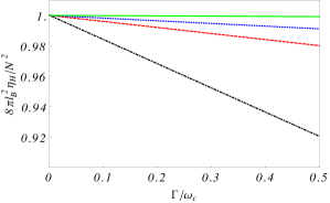
Figure 3: The normalized Hall viscosity, $8\pi l_{B}^{2}\eta_{H}/N^{2}$, as the function of $\Gamma/\omega_{c}$ for different ranges of disorder in the case of well-separated LLs. The parameter $\tau_{\rm tr,2}/\tau_{0}$ is equal to $1$, $2$, $3$, and $10$ from the bottom to the top.

In the case of overlapping LLs, $\omega_{c}\tau_{0}\ll 1$, from Eq.(15) we obtain the Shubnikov-de Haas oscillations of the Hall viscosity:

$$\eta_{\rm H}=\frac{\nu_{0}\mu^{2}\omega_{c}\tau_{\rm tr,2}^{2}}{1+4\alpha^{2}}\left(1+\frac{\delta}{2\alpha^{2}}\frac{1+12\alpha^{2}}{1+4\alpha^{2}}\mathcal{F}_{T}\cos\frac{2\pi\mu}{\omega_{c}}\right).$$ (16)

The non-oscillatory term in $\eta_{\rm H}$ coincides with the classical result for the Hall viscosity of electron gas Steinberg .

In the case of well-separated LLs, $\omega_{c}\tau_{0}\gg 1$, one finds from Eq. (15) that the Hall viscosity is reduced from the quantized value if the chemical potential lies within the broadened LL, $|\mu-\epsilon_{N}|\leqslant\Gamma$:

$$\eta_{H}=\frac{N^{2}}{8\pi l_{B}^{2}}\left[1-\frac{\tau_{0}^{2}\Gamma}{2\pi\omega_{c}\tau_{\rm tr,2}^{2}}\left(1-\frac{(\mu-\epsilon_{N})^{2}}{\Gamma^{2}}\right)^{3/2}\right].$$ (17)

We note that for the long-range-correlated random potential the Hall viscosity dominates the shear viscosity, $\eta_{H}\gg\eta_{s}$ (cf. Eqs. (10) and (17)).

The deviation of the Hall viscosity from the clean value is controlled by the small parameter $(\tau_{0}/\tau_{\rm tr,2})^{2}/\sqrt{\omega_{c}\tau_{0}}\ll 1$. In the case of short range random potential correlations, $\tau_{0}=\tau_{\rm tr,2}$, the deviation of $\eta_{H}$ from its clean value is very small. For long-range-correlated random potential, $\tau_{0}\ll\tau_{\rm tr,2}$, the difference $\eta_{H}-N^{2}/(8\pi l_{B}^{2})$ is additionally suppressed (see Fig. 3).

Numerical results. — We would now like to explore the quantum Hall regime, where the number of filled LLs is of order unity. Here the SCBA cannot be used anymore, and we resort to a numerical calculation. For this we discretize the system and employ the Hofstadter model with uncorrelated random potential, uniformly distributed between $[-w/2,w/2]$ at each lattice site. We calculate the Hall viscosity at zero temperature using retarded correlation function of discretized stress operators TuegelHueghes , and take both the continuum and thermodynamic limits to extrapolate to the behavior of our model (1) SM . In the presence of disorder we can take these limits while keeping constant $\omega_{c}\tau$. The results for the Hall viscosity are plotted in Fig. 4, together with the behavior of the Hall conductivity ($\sigma_{H}$) at zero wavevector. One sees that, somewhat surprisingly, the Hall viscosity maintains its quantization to the same extent as the Hall conductivity, that is, until the quantum Hall to insulator transition is approached.

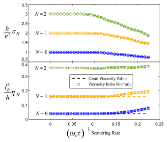
Figure 4: The Hall conductivity (circles) and viscosity (squares) as function of $\omega_{c}\tau$ for $N=0,1$, and $2$ filled Landau levels (blue, yellow, and green, respectively). The clean viscosity values are also indicated by dashed lines. $\eta_{H}$ is seen to be robust to disorder to the same extent the $\sigma_{H}$ is, within the numerical errors (error bars are smaller than the symbol sizes.)

Conclusions. — To summarize, we studied the dissipative and Hall viscosity of 2D electron system in the presence of a random potential. Within the self-consistent Born approximation we derived an expressions for both the dissipative and Hall viscosities, which takes into account the modification of the single-particle density of states and the elastic transport time due to the Landau quantization. Our results smoothly interpolate between the case of weak magnetic field and strong disorder, on the one hand, and the case of strong magnetic field and vanishing disorder, on the other hand. In the former regime, we derived the expressions for the quantum (Shubnikov-de Haas type) oscillations of the dissipative and Hall viscosities. In the case of strong magnetic field, we found that the disorder broadening of the Landau level does not lead to a significant change of the Hall viscosity in comparison with the clean result. Our numerical results for a few filled LLs support this striking conclusion.

There are various ways to extend our work. In Galilean invariant systems it was proven Hoyos ; Bradlyn2012 that the viscosity tensor can be extracted from the nonlocal conductivity, that is, the conductivity tensor at finite wave-vector $\bm{q}$. In the absence of Galilean invariance there is no reason to expect that $\eta_{H}$ is related to $\sigma_{H}(\bm{q})$ Radzihovsky ; HollerRead . Also, the relation between $\eta_{H}$ and $\sigma_{H}(\bm{q})$ can be affected by the presence of a lattice TuegelHueghes ; Harper2018 or disorder. However, if one treats disorder on the level of Drude model with classical magnetic field, the relation of Ref. Bradlyn2012 between $\eta_{H}$ and $\sigma_{H}(\bm{q})$ still holds HKO . This fact is not surprising since the Drude model does not properly take into account the LLs, which result in the energy dependence of the density of states and elastic scattering transport time. However, such a simplification can be dangerous since $\eta_{H}$ and $\sigma_{H}$ have contributions coming from the states well below the Fermi energy. It would therefore be worthwhile to extend the presented analytical and numerical approaches to the conductivity at finite wave vector elsewhere . We also note that our techniques can be applied to calculation of the dissipative and Hall viscosity in graphene, where only the result in the absence of disorder is known SPV .

Acknowledgements. — We thank A. Abanov, O. Andreev, I. Gornyi, A. Mirlin, D. Polyakov, and P. Wiegmann for useful discussions. Hospitality by Tel Aviv University, the Weizmann Institute of Science, the Landau Institute for Theoretical Physics, and the Karlsruhe Institute of Technology is gratefully acknowledged. The work was partially supported by the Russian Foundation for Basic Research under Grant No. 17-02-00541, the program “Contemporary problems of low-temperature physics” of Russian Academy of Science, the Israel Ministry of Science and Technology (Contract No. 3-12419), the Israel Science Foundation (Grant No. 227/15), the German Israeli Foundation (Grant No. I-1259-303.10), the US-Israel Binational Science Foundation (Grant No. 2016224), and a travel grant by the BASIS Foundation.

in 1,…,10 See pages \x of PRL_Supplement_new_v5.pdf

References

- (1) R. N. Gurzhi, Hydrodynamics effects in solids at low temperature, Usp. Fiz. Nauk 94, 689 (1968) [Sov. Phys. Usp. 11, 255 (1968)].
- (2) M. J. M. de Jong and L. W. Molenkamp, Hydrodynamic electron flow in high-mobility wires, Phys. Rev. B 51, 13389 (1995).
- (3) M. Müller, J. Schmalian, and L. Fritz, Graphene: A nearly perfect fluid, Phys. Rev. Lett. 103, 025301 (2009).
- (4) A. V. Andreev, S. A. Kivelson, and B. Spivak, Hydrodynamic description of transport in strongly correlated electron systems, Phys. Rev. Lett. 106, 256804 (2011).
- (5) I. Torre, A. Tomadin, A. K. Geim, and M. Polini, Nonlocal transport and the hydrodynamic shear viscosity in graphene, Phys. Rev. B 92, 165433 (2015).
- (6) L. Levitov and G. Falkovich, Electron viscosity, current vortices and negative nonlocal resistance in graphene, Nature Physics 12, 672 (2016).
- (7) B. N. Narozhny I. V. Gornyi A. D. Mirlin, J. Schmalian, Hydrodynamic approach to electronic transport in graphene, Ann. Phys. (Berlin) 529, 1700043 (2017).
- (8) H. Guo, E. Ilseven, G. Falkovich, L. Levitov, Higher-than-ballistic conduction of viscous electron flows, PNAS 114, 3068 (2017).
- (9) O. Kashuba, B. Trauzettel, and L. W. Molenkamp, Relativistic Gurzhi effect in channels of Dirac materials, Phys. Rev. B 97, 205129 (2018).
- (10) A. Lucas and K. Ch. Fong, Hydrodynamics of electrons in graphene, J. Phys.: Condens. Matter 30, 053001 (2018).
- (11) E. I. Kiselev, J. Schmalian, The boundary conditions of viscous electron flow, arXiv: 1806.03933.
- (12) M. Titov, R. V. Gorbachev, B. N. Narozhny, T. Tudorovskiy, M. Schütt, P. M. Ostrovsky, I. V. Gornyi, A. D. Mirlin, M. I. Katsnelson, K. S. Novoselov, A. K. Geim, and L. A. Ponomarenko, Giant magnetodrag in graphene at charge neutrality, Phys. Rev. Lett. 111, 166601 (2013).
- (13) D. A. Bandurin, I. Torre, R. Krishna Kumar, M. Ben Shalom, A. Tomadin, A. Principi, G. H. Auton, E. Khestanova, K. S. Novoselov, I. V. Grigorieva, L. A. Ponomarenko, A. K. Geim, M. Polini, Negative local resistance caused by viscous electron backflow in graphene, Science 351, 1055 (2016).
- (14) J. Crossno, J. K. Shi, K. Wang, X. Liu, A. Harzheim, A. Lucas, S. Sachdev, P. Kim, T. Taniguchi, K. Watanabe, T. A. Ohki, K. Ch. Fong, Observation of the Dirac fluid and the breakdown of the Wiedemann-Franz law in graphene, Science 351, 1058 (2016).
- (15) P. J. W. Moll, P. Kushwaha, N. Nandi, B. Schmidt, A. P. Mackenzie, Evidence for hydrodynamic electron flow in PdCoO2, Science 351, 1061 (2016).
- (16) R. Krishna Kumar, D. A. Bandurin, F. M. D. Pellegrino, Y. Cao, A. Principi, H. Guo, G. H. Auton, M. Ben Shalom, L. A. Ponomarenko, G. Falkovich, K. Watanabe, T. Taniguchi, I. V. Grigorieva, L. S. Levitov, M. Polini, A. K. Geim, Superballistic flow of viscous electron fluid through graphene constrictions, Nature Physics 13, 1182 (2017).
- (17) D. A. Bandurin, A. V. Shytov, G. Falkovich, R. Krishna Kumar, M. Ben Shalom, I. V. Grigorieva, A. K. Geim, L. S. Levitov, Probing maximal viscous response of electronic system at the onset of fluidity, arXiv:1806:03231.
- (18) G. M. Gusev, A. D. Levin, E. V. Levinson, A. K. Bakarov, Viscous transport and Hall viscosity in a two-dimensional electron system, Phys. Rev. B 98, 161603(R) (2018).
- (19) S. Chapman and T. G. Cowling, “The mathematical theory of non-uniform gases”, Cambridge University Press, New York (1953).
- (20) W. Marshall, “Kinetic theory of an ionized gas”, AERE T/R 2419, Harwell, Berkshire (1958).
- (21) A. N. Kaufman, “Plasma viscosity in a magnetic field”, Physics of Fluids 3, 610 (1960).
- (22) W. B. Thompson, “The dynamics of high temperature plasma”, Rep. Prog. Phys. 24, 363 (1961).
- (23) S. I. Braginskii, Transport processes in plasma, Ed. M. A. Leontovich, vol.1, p. 183 Gosatomizdat, Moscow (1963)
- (24) M. S. Steinberg, Viscosity of electron gas in metals, Phys. Rev. 109, 1486 (1958).
- (25) J. E. Avron, R. Seiler, P. G. Zograf, Viscosity of quantum fluids, Phys. Rev. Lett. 75, 697 (1995).
- (26) P. Lévay, Berry phases for Landau Hamiltonians on deformed tori, J. Math. Phys. 36, 2792 (1995).
- (27) J. E. Avron, Odd viscosity, J. Stat. Phys. 92, 543 (1998).
- (28) N. Read, Non-Abelian adiabatic statistics and Hall viscosity in quantum Hall states and paired superfluids, Phys. Rev. B 79, 045308 (2009).
- (29) N. Read and E. H. Rezayi, Hall viscosity, orbital spin, and geometry: Paired superfluids and quantum Hall systems, Phys. Rev. B 84, 085316 (2011).
- (30) F. D. M. Haldane, “Hall viscosity” and intrinsic metric of incompressible fractional Hall fluids, arXiv:0906.1854 (unpublished)
- (31) T. L. Hughes, R. G. Leigh, and E. Fradkin, Torsional response and dissipationless viscosity in topological insulators, Phys. Rev. Lett. 107, 075502 (2011).
- (32) C. Hoyos and D. T. Son, Hall viscosity and electromagnetic response, Phys. Rev. Lett. 108, 066805 (2012).
- (33) A. G. Abanov, On the effective hydrodynamics of the fractional quantum Hall effect, J. Phys. A: Math. Theor. 46, 292001 (2013).
- (34) A. G. Abanov and A. Gromov, Electromagnetic and gravitational responses of two-dimensional noninteracting electrons in a background magnetic field, Phys. Rev. B 90, 014435 (2014).
- (35) A. Gromov and A. G. Abanov, Density-curvature response and gravitational anomaly, Phys. Rev. Lett. 113, 266802 (2014).
- (36) C. Hoyos, Hall viscosity, topological states and effective theories, IJMP B 28, 14300007 (2014).
- (37) O. Andreev, M. Haack, and S. Hofmann, On nonrelativistic diffeomorphism invariance, Phys. Rev. D 89, 064012 (2014).
- (38) T. Can, M. Laskin, and P. Wiegmann, Fractional quantum Hall effect in a curved space: Gravitational anomaly and electromagnetic response, Phys. Rev. Lett. 113, 046803 (2014).
- (39) A. Gromov and A. G. Abanov, Thermal Hall effect and geometry with torsion, Phys. Rev. Lett. 114, 016802 (2015).
- (40) T. Can, M. Laskin, P. B. Wiegmann, Geometry of quantum Hall states: Gravitational anomaly and transport coefficients, Ann. Phys. (N.Y.) 362, 752 (2015).
- (41) V. Gurarie, Topological invariant for the orbital spin of the electrons in the quantum Hall regime and Hall viscosity, J. Phys.: Condens. Matter 27, 075601 (2015).
- (42) O. Andreev, More on nonrelativistic diffeomorphism invariance , Phys. Rev. D 91, 024035 (2015).
- (43) D. X. Nguyen and A. Gromov, Exact electromagnetic response of Landau level electrons , Phys. Rev. B 95, 085151 (2017).
- (44) Dung Xuan Nguyen, Tankut Can, and Andrey Gromov, Particle-hole duality in the lowest Landau level , Phys. Rev. Lett. 118, 206602 (2017).
- (45) P. S. Alekseev, Negative magnetoresistance in viscous flow of two-dimensional electrons, Phys. Rev. Lett. 117, 166601 (2016).
- (46) F. M. D. Pellegrino, I. Torre, and M. Polini, Nonlocal transport and the Hall viscosity of two-dimensional hydrodynamic electron liquids, Phys. Rev. B 96, 195401 (2017).
- (47) T. Scaffidi, N. Nandi, B. Schmidt, A. P. Mackenzie, and J. E. Moore, Hydrodynamic electron flow and Hall viscosity, Phys. Rev. Lett. 118, 226601 (2017).
- (48) L. V. Delacrétaz and A. Gromov, Transport signatures of the Hall viscosity, Phys. Rev. Lett. 119, 226602 (2017).
- (49) S. Ganeshan and A. G. Abanov, Odd viscosity in two-dimensional incompressible fluids , Phys. Rev. Fluids 2, 094101 (2017).
- (50) P. S. Alekseev, A. P. Dmitriev, I. V. Gornyi, V. Yu. Kachorovskii, B. N. Narozhny, M. Titov, Nonmonotonic magnetoresistance of a two-dimensional viscous electron-hole fluid in a confined geometry, Phys. Rev. B 97, 085109 (2018).
- (51) A. I. Berdyugin, S. G. Xu, F. M. D. Pellegrino, R. Krishna Kumar, A. Principi, I. Torre, M. Ben Shalom, T. Taniguchi, K. Watanabe, I. V. Grigorieva, M. Polini, A. K. Geim, D. A. Bandurin, Measuring Hall viscosity of graphene’s electron fluid, arXiv:1806.01606.
- (52) A. G. Abanov, T. Can, and S. Ganeshan, Odd surface waves in two-dimensional incompressible fluids, SciPost Phys. 5, 10 (2018).
- (53) A. Souslov, K. Dasbiswas, S. Vaikuntanathan, and V. Viteli, Topological waves and odd viscosity in chiral active fluids and plasmas, Phys. Rev. Lett. 122, 128001 (2019).
- (54) R. Cohen and M. Goldstein, Hall and dissipative viscosity effects on edge magnetoplasmons, Phys. Rev. B 98, 235103 (2018).
- (55) T. Ando, A. B. Fowler, and F. Stern, Electronic properties of 2D systems, Rev. Mod. Phys. 54, 437 (1982).
- (56) B. Bradlyn, M. Goldstein, and N. Read, Kubo formulas for viscosity: Hall viscosity, Ward identities, and the relation with conductivity, Phys. Rev. B 86, 245309 (2012).
- (57) P. M. V. Résibois and M. de Leener, Classical kinetic theory of fluids, Wiley (1977)
- (58) J. A. McLennan Jr., Statistical mechanics of transport in fluids, Phys. Fluids 3, 493 (1960).
- (59) See the detailed discussion of the internal compressibility in Ref. Bradlyn2012 .
- (60) J. H. Irving and J. G. Kirkwood,The statistical mechanical theory of transport processes. IV. The equations of hydrodynamics, J. Chem. Phys. 18, 817 (1950).
- (61) See the Supplemental Material for more details on the derivations and the numerical procedure.
- (62) M. E. Raikh and T.V. Shahbazyan, High Landau levels in a smooth random potential for two-dimensional electrons, Phys. Rev. B 47, 1522 (1993).
- (63) B. Laikhtman and E. L. Altshuler, Quasiclassical Theory of Shubnikov-de Haas Effect in 2D Electron Gas, Ann. Phys. (N.Y.) 232, 332 (1994).
- (64) I. A. Dmitriev, A. D. Mirlin, D. G. Polyakov, Cyclotron-resonance harmonics in the ac response of a 2D electron gas with smooth disorder, Phys. Rev. Lett. 91, 226802 (2003).
- (65) Up to small mesoscopic fluctuations (see, e.g., Ref. anisovich87 for the case of the thermopower), as we have also verified numerically.
- (66) A. V. Anisovich, B. L. Altshuler, A. G. Aronov, and A. Yu. Zyuzin, Mesoscopic fluctuations of thermoelectric coefficients, Pis’ma Zh. Eksp. Teor. Fiz. 45, 237 (1987) [JETP Lett. 45, 295 (1987)].
- (67) L. Smrčka and P. Středa, Transport coefficients in strong magnetic field, J. Phys. C: Solid State Phys. 10, 2153 (1977).
- (68) Y. Hidaka, Y. Hirono, T. Kimura, Y. Minami, Viscoelastic-electromagnetism and Hall viscosity, PTEP 1, 013A02 (2013).
- (69) E.M. Lifshitz and L. P. Pitaevskii, Course of Theoretical Physics, vol. 10, Physical Kinetics, Pergamon Press (1981).
- (70) I. A. Dmitriev, A. D. Mirlin, D. G. Polyakov, M. A. Zudov, Nonequilibrium phenomena in high Landau levels, Rev. Mod. Phys. 84, 1709 (2012).
- (71) T. I. Tuegel and T. L. Hughes, Hall viscosity and momentum transport in lattice and continuum models of the integer quantum Hall effect in strong magnetic fields, Phys. Rev. B 92, 165127 (2015).
- (72) S. Moroz, C. Hoyos, and L. Radzihovsky, Galilean invariance at quantum Hall edge , Phys. Rev. B 91, 195409 (2015); Phys. Rev. B 96, 039902 (2017).
- (73) J. Höller and N. Read, Comment on “Galilean invariance at quantum Hall edge”, Phys. Rev. B 93, 197401 (2016).
- (74) F. Harper, D. Bauer, T. S. Jackson, and R. Roy, Finite-wave-vector electromagnetic response in lattice quantum Hall systems, Phys. Rev. B 98, 245303 (2018).
- (75) C. Hoyos, B. S. Kim, Y. J. Oz, Ward identities for Hall transport, High Energ. Phys. 2014: 54 (2014).
- (76) I. S. Burmistrov, M. Goldstein, M. Kot, P. D. Kurilovich, V. D. Kurilovich, in preparation.
- (77) M. Sherafati, A. Principi, and G.Vignale, Hall viscosity and electromagnetic response of electrons in graphene, Phys. Rev. B 94, 125427 (2016).