See pages - of final_manuscript.pdf

Supplementary Material

1 Simulations - Error in Estimated Trajectories and DPS

Figure 1: Error in DPS scores (A) and trajectory estimation (B) for Scenario 2 in simulation experiments. (C-D) The same error scores for Scenario 3. We notice that as the problem becomes more difficult, the errors in the DIVE estimated parameters increase. Errors were measured as sum of squared differences (SSD) between the true parameters and estimated parameters. For the trajectories, the SSD was calculated only based on the sigmoid centres, due to different scaling of the other sigmoidal parameters.

2 Comparison between DIVE and other models

2.1 Motivation

We were also interested to compare the performance of DIVE with other disease progression models. In particular, we were interested to test whether:

• Modelling dynamic clusters on the brain surface improves subject staging and biomarker prediction

• Modelling subject-specific stages with a linear transformation (the $\alpha_{i}$ and $\beta_{i}$ terms) improves biomarker prediction

2.2 Experiment design

We compared the performance of our model to two simplified models:

• ROI-based model: groups vertices according to an a-priori defined ROI atlas. This model is equivalent to the model by Jedynak et al., Neuroimage, 2012 and is a special case of our model, where the latent variables $z_{lk}$ are fixed instead of being marginalised as in equation 6.

• No-staging model: This is a model that doesn’t perform any time-shift of patients along the disease progression timeline. It fixes $\alpha_{i}=1$, $\beta_{i}=0$ for every subject, which means that the disease progression score of every subject is age.

We performed this comparison using 10-fold cross-validation. For each subject in the test set, we computed their DPS score and correlated all the DPS values with the same four cognitive tests used previously. We also tested how well the models can predict the future vertex-wise measurements as follows: for every subject i in the test set, we used their first two scans to estimate $\alpha_{i}=1$, $\beta_{i}=0$ and then used the rest of the scans to compute the prediction error. For one vertex location on the cortical surface, the prediction error was computed as the root mean squared error (RMSE) between its predicted measure and the actual measure. This was then averaged across all subjects and visits.

2.3 Results

Table 1 shows the results of the model comparison, on ADNI MRI dataset. Each row represents one model tested, while each column represents a different performance measure: correlations with four different cognitive tests and accuracy in the prediction of future vertexwise measurements. In each entry, we give the mean and standard deviation of the correlation coefficients or RMSE across the 10 cross-validation folds.

Model	CDRSOB ($\rho$)	ADAS13 ($\rho$)	MMSE ($\rho$)	RAVLT ($\rho$)	Prediction (RMSE)
DIVE	0.37 +/- 0.09	0.37 +/- 0.10	0.36 +/- 0.11	0.32 +/- 0.12	1.021 +/- 0.008
ROI-based model	0.36 +/- 0.10	0.35 +/- 0.11	0.34 +/- 0.13	0.30 +/- 0.13	1.019 +/- 0.010
No-staging model	*0.09 +/- 0.06	*0.03 +/- 0.09	*0.05 +/- 0.06	*0.02 +/- 0.06	*1.062 +/- 0.024

Table 1: Comparison of our model with two more simplistic models on the ADNI MRI dataset. For each of the three models, we show the correlation of the disease progression scores (DPS) with respect to several cognitive tests: CDRSOB, ADAS13, MMSE and RAVLT. The correlation numbers represent the mean correlation across the 10 cross-validation folds.

3 Validation of subject parameters against APOE

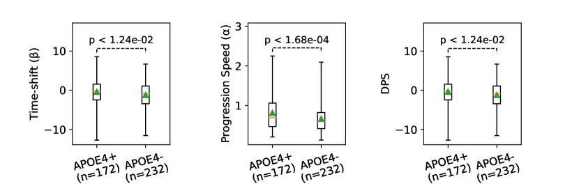
Figure 2: Subject-specific parameters (left: time shift parameters $\beta$, middle: progression speed $\alpha$ and right: DPS scores at baseline visit) for APOE4-positive and negative individuals. APOE4 positive subjects have significantly higher time-shifts, progression speeds and overall DPS scores than APOE4-negative individuals.

4 Derivation of the Generalised EM algorithm

We seek to calculate $M^{(u)}=\operatorname*{arg\,max}_{M}\mathbb{E}_{Z|V,M^{(u-1)}}\left[log\ p(V,Z|M)\right]+log\ p(M)$ where $M^{(u)}=(\alpha^{(u)},\beta^{(u)},\theta^{(u)},\sigma^{(u)},\lambda^{(u)})$ are the set of model parameters at iteration $u$ of the EM algorithm, and $Z=(Z_{1},\dots,Z_{L})$ is the set of discrete latent variables, where $Z_{l}$ represents the cluster that voxel $l$ was assigned to, so $Z_{l}\in{1,\dots,K}$. While $Z_{l}$ (with capital letter) is a random variable, we will also use the notation $z_{l}$ (small letter) to represent the value that the random variable $Z_{l}$ was instantiated to. Finally, $p(M^{(u)})$ is a prior on these parameters that is chosen by the user. Expanding the expected value, we get:

$$M^{(u)}=\operatorname*{arg\,max}_{M}\sum_{z1,\dots,z_{L}}^{K}p(Z=(z_{1},...,z_{L})|V,M^{(u-1)})\left[log\ p(V,Z|M)\right]+log\ p(M)$$ (1)

The E-step involves computing $p\left(Z=(z_{1},...,z_{L})|V,M^{(u-1)}\right)$, while the M-step comprises of solving the above equation.

4.1 E-step

In this step we need to estimate $p(Z|V,M^{(u-1)})$. For notational simplificy we will drop the $(u-1)$ superscript from $M$

$$p(Z|V,M)=\frac{1}{C}p(V,Z|M)=\prod_{l}^{L}\left[\prod_{(i,j)\in I}N(V_{l}^{ij}|f(\alpha_{i}t_{ij}+\beta_{i}|\theta_{Z_{l}}),\sigma_{Z_{l}})\prod_{l_{2}\in N_{l}}\Psi(Z_{l},Z_{l_{2}})\right]$$ (2)

where $N_{l}$ is the set of neighbours of vertex $l$. However, this doesn’t directly factorise over the vertices $l$ due to the MRF terms $\Psi(Z_{l},Z_{l_{2}})$. It is however necessary to find a form that factorises over the vertices, otherwise we won’t be able to represent in memory the joint distribution over all $Z$ variables. If we make the approximation $p(Z|V,M)\approx\prod_{l}^{L}p(V_{l}|Z_{l},M)$ then we loose out all the MRF terms and the model won’t account for spatial correlation. We instead do a first-degree approximation by conditioning on the values of $Z_{N_{l}}^{(u-1)}$, the labels of nearby vertices from the previous iteration. The approximation is thus:

$$p(Z|V,M)\approx\prod_{l}^{L}\mathbb{E}_{Z_{N_{l}}^{(u-1)}|V_{l},M}\left[p(Z_{l}|V_{l},M,Z_{N_{l}}^{(u-1)})\right]$$ (3)

This form allows us to factorise over all the vertices to get $p(Z_{l}|V_{l},M)$:

$$p(Z_{l}|V_{l},M)\approx\frac{1}{C}\sum_{Z_{N_{l}}^{(u-1)}}p(V_{l}|Z_{l},M)p(Z_{l}|Z_{N_{l}}^{(u-1)})p(Z_{N_{l}}^{(u-1)}|V_{l},M)$$ (4)

where $C$ is a normalistion constant that can be dropped. We can now further factorise $p(Z_{l}|Z_{N_{l}}^{(u-1)})\approx\prod_{m\in\{1,...,N_{l}\}}p(Z_{l}|M,Z_{N_{l}(m)}^{(u-1)}=z_{N_{l}(m)})$ and apply a similar factorisation to the prior $p(Z_{N_{l}}^{(u-1)}|V_{l},M)$, resulting in:

$$p(Z_{l}|V_{l},M)\approx\frac{1}{C}p(V_{l}|Z_{l},M)\sum_{z_{N_{l}(1)},..,z_{N_{l}(|N_{l}|)}}\ \ \ \prod_{m\in\{1,...,N_{l}\}}p(Z_{l}|Z_{N_{l}(m)}^{(u-1)}=z_{N_{l}(m)})p(Z_{N_{l}(m)}^{(u-1)}=z_{N_{l}(m)}|V_{l},M)$$ (5)

Factorising the summation over $z_{N_{l}}$’s we get:

$$p(Z_{l}|V_{l},M)=p(V_{l}|Z_{l},M)\prod_{l_{2}\in N_{l}}\sum_{z_{l_{2}}}p(Z_{l}|Z_{l_{2}}^{(u-1)}=z_{l_{2}})p(Z_{l_{2}}^{(u-1)}=z_{l_{2}}|V_{l},M)$$ (6)

Replacing $z_{l_{2}}$ with $k_{2}$ we get:

$$p(Z_{l}|V_{l},M)=p(V_{l}|Z_{l},M)\prod_{l_{2}\in N_{l}}\sum_{k_{2}}p(Z_{l}|Z_{l_{2}}^{(u-1)}=k_{2})p(Z_{l_{2}}^{(u-1)}=k_{2}|V_{l},M)$$ (7)

We shall also denote $z_{lk}=p(Z_{l}|V_{l},M)$. Further simplifications result in:

$$z_{lk}^{(u)}\propto\left[\prod_{i,j\in I}N(V_{l}^{ij}|f(\alpha_{i}t_{ij}+\beta_{i};\theta_{k}),\sigma_{k})\right]\left[\prod_{l_{2}\in N_{l}}\sum_{k_{2}=1}^{K}z_{l_{2}k_{2}}^{(u-1)}\ \Psi(Z_{l}=k,Z_{l_{2}}=k_{2})\right]$$ (8)

$$log\ z_{lk}^{(u)}\propto\left[\sum_{i,j\in I}-\frac{log\ (2\pi\sigma_{k}^{2})}{2}-\frac{1}{2\sigma_{k}^{2}}(V_{l}^{ij}-f(\alpha_{i}t_{ij}+\beta_{i};\theta_{k}))^{2}\right]+\left[\sum_{l_{2}\in N_{l}}log\sum_{k_{2}=1}^{K}z_{l_{2}k_{2}}^{(u-1)}(\delta_{k_{2}k}\ exp(\lambda)+(1-\delta_{k_{2}k})\ exp(-\lambda^{2}))\right]$$ (9)

We further define the data-fit term $D_{lk}$ as follows:

$$D_{lk}=-\frac{log\ (2\pi\sigma_{k}^{2})|I|}{2}-\sum_{i,j\in I}\frac{1}{2\sigma_{k}^{2}}(V_{l}^{ij}-f(\alpha_{i}t_{ij}+\beta_{i};\theta_{k}))^{2}$$ (10)

This results in:

$$log\ z_{lk}^{(u)}\propto D_{lk}+\left[\sum_{l_{2}\in N_{l}}log\sum_{k_{2}=1}^{K}z_{l_{2}k_{2}}^{(u-1)}(\delta_{k_{2}k}\ (exp(\lambda)-exp(-\lambda^{2}))+exp(-\lambda^{2}))\right]$$ (11)

Finally, we simplify the sum over $k_{2}$ to get the update equation for $z_{lk}$:

$$\begin{split}log\ z_{lk}^{(u)}\propto D_{lk}+\left[\sum_{l_{2}\in N_{l}}log\ \left[exp(-\lambda^{2})+z_{l_{2}k}^{(u-1)}(exp(\lambda)-exp(-\lambda^{2}))\right]\right]\end{split}$$ (12)

In practice, we cannot naively compute the exponential term $z_{lk}=exp(log(z_{lk}))$ due to precision loss. However, we go around this by recomputing the exponentiation and normalisation of $z_{lk}$ simultaneously. Denoting $x(k)=log\ z_{lk}$, for $k\in[1\dots K]$, we get:

$$z_{lk}=\frac{e^{x(k)}}{e^{x(1)}+e^{x(2)}+\dots+e^{x(K)}}=\frac{1}{e^{x(1)-x(k)}+e^{x(2)-x(k)}+\dots+e^{x(K)-x(k)}}$$ (13)

4.2 M-step

The M-step itself does not have a closed-form analytical solution. We choose to solve it by successive refinements of the cluster trajectory parameters and the subject time shifts.

4.2.1 Optimising trajectory parameters

Trajectory shape - $\theta$

Taking equation 1 and fixing the subject time-shifts $\alpha$, $\beta$ and measurement noise $\sigma$, we can find its maximum with respect to $\theta$ only. More precisely, we want:

$$\theta=\operatorname*{arg\,max}_{\theta}\sum_{z1,\dots,z_{L}}^{K}p(Z=(z_{1},...,z_{L})|V,M^{(u-1)})\left[log\ p(V,Z|M)\right]+log\ p(\theta)$$ (14)

We observe that for each cluster the individual $\theta_{k}$’s are conditionally independent, i.e. $\theta_{k}\perp\!\!\!\perp\theta_{m}|\{Z,\alpha,\beta,\sigma$} $\forall k,m$. We also assume that the prior factorizes for each $\theta_{k}$: $\log p(\theta)=\prod_{k}^{K}\log p(\theta_{k})$. This allows us to optimise each $\theta_{k}$ independently:

$$\theta_{k}=\operatorname*{arg\,max}_{\theta_{k}}\sum_{z1,\dots,z_{L}}^{K}p(Z=(z_{1},...,z_{L})|V,M^{(u-1)})\left[log\ p(V,Z|M)\right]+log\ p(\theta_{k})$$ (15)

Replacing the full data log-likelihood, we get:

$$\theta_{k}=\operatorname*{arg\,max}_{\theta_{k}}\sum_{z1,\dots,z_{L}}^{K}p(Z=(z_{1},...,z_{L})|V,M^{(u-1)})\ log\left[\prod_{l=1}^{L}\prod_{(i,j)\in I}N(V_{l}^{ij}|f(\alpha_{i}t_{ij}+\beta_{i};\theta_{z_{l}}),\sigma_{z_{l}})\right]+log\ p(\theta_{k})$$ (16)

Note that we didn’t include the MRF clique terms, since they are not a function of $\theta_{k}$. We propagate the logarithm inside the products:

$$\theta_{k}=\operatorname*{arg\,max}_{\theta_{k}}\sum_{z1,\dots,z_{L}}^{K}p(Z=(z_{1},...,z_{L})|V,M^{(u-1)})\sum_{l=1}^{L}\sum_{(i,j)\in I}log\ N(V_{l}^{ij}|f(\alpha_{i}t_{ij}+\beta_{i};\theta_{z_{l}}),\sigma_{z_{l}})+log\ p(\theta_{k})$$ (17)

We next assume that $Z_{l}$, the hidden cluster assignment for vertex $l$, is conditionally independent of the other vertex assignments $Z_{m}$, $\forall m\neq l$ (See E-step approximation from Eq. 3). This independence assumption induces the following factorization: ${p(Z=(z_{1},...,z_{L})|V,M^{(u-1)})=\prod_{l}^{L}p(Z_{l}=z_{l}|V,M^{(u-1)})}$. Propagating this product inside the sum over the vertices, we get:

$$\theta_{k}=\operatorname*{arg\,max}_{\theta_{k}}\sum_{l=1}^{L}\sum_{z_{l}=1}^{K}p(Z_{l}=z_{l}|V,M^{(u-1)})\sum_{(i,j)\in I}log\ N(V_{l}^{ij}|f(\alpha_{i}t_{ij}+\beta_{i};\theta_{z_{l}}),\sigma_{z_{l}})+log\ p(\theta_{k})$$ (18)

The terms which don’t contain $\theta_{k}$ dissapear:

$$\theta_{k}=\operatorname*{arg\,max}_{\theta_{k}}\sum_{l=1}^{L}p(Z_{l}=k|V,M^{(u-1)})\sum_{(i,j)\in I}log\ N(V_{l}^{ij}|f(\alpha_{i}t_{ij}+\beta_{i};\theta_{k}),\sigma_{k})+log\ p(\theta_{k})$$ (19)

We further expand the gaussian noise model:

$$\theta_{k}=\operatorname*{arg\,max}_{\theta_{k}}\sum_{l=1}^{L}p(Z_{l}=k|V,M^{(u-1)})\sum_{(i,j)\in I}\left[log\ (2\pi\sigma_{k})^{-1/2}-\frac{1}{2\sigma_{k}^{2}}(V_{l}^{ij}-f(\alpha_{i}t_{ij}+\beta_{i};\theta_{k}))^{2}\right]+log\ p(\theta_{k})$$ (20)

Constants dissapear due to the $\operatorname*{arg\,max}$ and we get the final update equation for $\theta_{k}$:

$$\theta_{k}=\operatorname*{arg\,max}_{\theta_{k}}\sum_{l=1}^{L}p(Z_{l}=k|V,M^{(u-1)})\sum_{(i,j)\in I}\left[-\frac{1}{2\sigma_{k}^{2}}(V_{l}^{ij}-f(\alpha_{i}t_{ij}+\beta_{i};\theta_{k}))^{2}\right]+log\ p(\theta_{k})$$ (21)

Measurement noise - $\sigma$

We first assume a uniform prior on the $\sigma$ parameters to simplify derivations. Using a similar approach as with $\theta$, after propagating the product inside the logarithm and removing the terms which don’t contain $\sigma_{k}$, we get:

$$\sigma_{k}=\operatorname*{arg\,max}_{\sigma_{k}}\sum_{l=1}^{L}p(Z_{l}=k|V,M^{(u-1)})\sum_{(i,j)\in I}log\ N(V_{l}^{ij}|f(\alpha_{i}t_{ij}+\beta_{i};\theta_{k}),\sigma_{k})$$ (22)

Note that, just as for $\theta$ above, the MRF clique terms were not included because they are not a function of $\sigma_{k}$. Expanding the noise model we get:

$$\sigma_{k}=\operatorname*{arg\,max}_{\sigma_{k}}\sum_{l=1}^{L}p(Z_{l}=k|V,M^{(u-1)})\sum_{(i,j)\in I}\left[log\ (2\pi\sigma_{k}^{2})^{-1/2}-\frac{1}{2\sigma_{k}^{2}}(V_{l}^{ij}-f(\alpha_{i}t_{ij}+\beta_{i};\theta_{k}))^{2}\right]$$ (23)

The maximum of a function $l(\sigma_{k})$ can be computed by taking the derivative of the function $l$ and setting it to zero. This is under the assumption that $l$ is differentiable, which it is but we won’t prove it here. This gives:

$$\frac{\delta l(\sigma_{k}|.)}{\delta\sigma_{k}}=\sum_{l=1}^{L}p(Z_{l}=k|V,M^{(u-1)})\sum_{(i,j)\in I}\frac{\delta}{\delta\sigma_{k}}\left[log\ (2\pi\sigma_{k}^{2})^{-1/2}-\frac{1}{2\sigma_{k}^{2}}(V_{l}^{ij}-f(\alpha_{i}t_{ij}+\beta_{i};\theta_{k}))^{2}\right]$$ (24)

Propagating the differential operator further inside the sums we get:

$$\frac{\delta l(\sigma_{k}|.)}{\delta\sigma_{k}}=\sum_{l=1}^{L}p(Z_{l}=k|V,M^{(u-1)})\sum_{(i,j)\in I}\left[-\frac{\delta}{\delta\sigma_{k}}\frac{log\ \sigma_{k}^{2}}{2}-\frac{\delta}{\delta\sigma_{k}}\frac{1}{2\sigma_{k}^{2}}(V_{l}^{ij}-f(\alpha_{i}t_{ij}+\beta_{i};\theta_{k}))^{2}\right]$$ (25)

We next perform several small manipulations to reach a more suitable form of the derivative and then set it to be equal to zero:

$$\frac{\delta l(\sigma_{k}|.)}{\delta\sigma_{k}}=\sum_{l=1}^{L}p(Z_{l}=k|V,M^{(u-1)})\sum_{(i,j)\in I}\left[-\frac{1}{\sigma_{k}}-\frac{-2}{2\sigma_{k}^{3}}(V_{l}^{ij}-f(\alpha_{i}t_{ij}+\beta_{i};\theta_{k}))^{2}\right]$$ (26)

$$\frac{\delta l(\sigma_{k}|.)}{\delta\sigma_{k}}=\sum_{l=1}^{L}p(Z_{l}=k|V,M^{(u-1)})\sum_{(i,j)\in I}\left[-\frac{\sigma_{k}^{2}}{\sigma_{k}^{3}}+\frac{1}{\sigma_{k}^{3}}(V_{l}^{ij}-f(\alpha_{i}t_{ij}+\beta_{i};\theta_{k}))^{2}\right]$$ (27)

$$\frac{\delta l(\sigma_{k}|.)}{\delta\sigma_{k}}=\sum_{l=1}^{L}p(Z_{l}=k|V,M^{(u-1)})\sum_{(i,j)\in I}\left[-\sigma_{k}^{2}+(V_{l}^{ij}-f(\alpha_{i}t_{ij}+\beta_{i};\theta_{k}))^{2}\right]=0$$ (28)

Finally, we solve for $\sigma_{k}$ and get its update equation:

$$\sigma_{k}^{2}=\frac{1}{|I|}\sum_{l=1}^{L}p(Z_{l}=k|V,M^{(u-1)})\sum_{(i,j)\in I}(V_{l}^{ij}-f(\alpha_{i}t_{ij}+\beta_{i};\theta_{k}))^{2}$$ (29)

4.2.2 Estimating subject time shifts - $\alpha$, $\beta$

For estimating $\alpha$, $\beta$, we adopt a similar strategy as in the case of $\theta$, up to Eq. 18. This gives us the following problem:

$$\alpha_{i},\beta_{i}=\operatorname*{arg\,max}_{\alpha_{i},\beta_{i}}\sum_{l=1}^{L}\sum_{k=1}^{K}p(Z_{l}=k|V,M^{(u-1)})\sum_{(i^{\prime},j)\in I}log\ N(V_{l}^{i^{\prime}j}|f(\alpha_{i^{\prime}}t_{i^{\prime}j}+\beta_{i^{\prime}};\theta_{k}),\sigma_{k})+log\ p(\alpha_{i},\beta_{i})$$ (30)

The terms $\alpha_{i^{\prime}},\beta_{i^{\prime}}$ for other subjects $i^{\prime}\neq i$ dissappear:

$$\alpha_{i},\beta_{i}=\operatorname*{arg\,max}_{\alpha_{i},\beta_{i}}\sum_{l=1}^{L}\sum_{k=1}^{K}p(Z_{l}=k|V,M^{(u-1)})\sum_{j\in I_{i}}log\ N(V_{l}^{ij}|f(\alpha_{i}t_{ij}+\beta_{i};\theta_{k}),\sigma_{k})+log\ p(\alpha_{i},\beta_{i})$$ (31)

Expanding the gaussian noise model we get:

$$\alpha_{i},\beta_{i}=\operatorname*{arg\,max}_{\alpha_{i},\beta_{i}}\sum_{l=1}^{L}\sum_{k=1}^{K}p(Z_{l}=k|V,M^{(u-1)})\sum_{j\in I_{i}}\left[log\ (2\pi\sigma_{k}^{2})^{-1/2}-\frac{1}{2\sigma_{k}^{2}}(V_{l}^{ij}-f(\alpha_{i}t_{ij}+\beta_{i};\theta_{k}))^{2}\right]+log\ p(\alpha_{i},\beta_{i})$$ (32)

After removing constant terms we end up with the final update equation for $\alpha_{i}$, $\beta_{i}$:

$$\alpha_{i},\beta_{i}=\operatorname*{arg\,min}_{\alpha_{i},\beta_{i}}\left[\sum_{l=1}^{L}\sum_{k=1}^{K}p(Z_{l}=k|V,M^{(u-1)})\frac{1}{2\sigma_{k}^{2}}\sum_{j\in I_{i}}(V_{l}^{ij}-f(\alpha_{i}t_{ij}+\beta_{i};\theta_{k}))^{2}\right]-log\ p(\alpha_{i},\beta_{i})$$ (33)

4.2.3 Estimating MRF clique term - $\lambda$

We optimise $\lambda$ using the following formula:

$$\lambda^{(u)}=\operatorname*{arg\,max}_{\lambda}E_{p(Z|V,M^{(u-1)},\lambda,Z^{(u-1)})}[log\ p(V,Z|M^{(u-1)})]$$

Note that $p(Z|V,M^{(u-1)},\lambda,Z^{(u-1)})$ is a function of $\lambda$, so for each lambda we estimate $z_{lk}$ through approximate inference. We do this because otherwise the optimisation of $\lambda$ will only take into account the clique terms and completely exclude the data terms. We further simplify the objective function for lambda as follows:

$$\lambda^{(u)}=\operatorname*{arg\,max}_{\lambda}\sum_{z1,\dots,z_{L}}^{K}p(Z=(z_{1},...,z_{L})|V,M^{(u-1)},\lambda,Z^{(u-1)})\ log\left[\prod_{l=1}^{L}\prod_{(i,j)\in I}N(V_{l}^{ij}|f(\alpha_{i}t_{ij}+\beta_{i};\theta_{z_{l}}),\sigma_{z_{l}})\prod_{l=1}^{L}\prod_{l_{2}\in N_{l}}\Psi(z_{l},z_{l_{2}})\right]$$

We take the logarithm:

$$\lambda^{(u)}=\operatorname*{arg\,max}_{\lambda}\sum_{z1,\dots,z_{L}}^{K}p(Z=(z_{1},...,z_{L})|V,M^{(u-1)},\lambda,Z^{(u-1)})\ \left[\sum_{l=1}^{L}\sum_{(i,j)\in I}log\ N(V_{l}^{ij}|..)+\sum_{l=1}^{L}\sum_{l_{2}\in N_{l}}log\ \Psi(z_{l},z_{l_{2}})\right]$$

Let us denote $z_{lk}=p(Z_{l}=k|V,M^{(u-1)},\lambda,Z^{(u-1)})$. Assuming independence between the latent variables $Z_{l}$ we get:

$$\lambda=\operatorname*{arg\,max}_{\lambda}\sum_{l=1}^{L}\sum_{k=1}^{K}z_{lk}\ \left[\sum_{(i,j)\in I}log\ N(V_{l}^{ij}|..)\right]+\sum_{l=1}^{L}\sum_{k=1}^{K}z_{lk}\sum_{l_{2}\in N_{l}}\sum_{k_{2}=1}^{K}z_{l_{2}k}\ log\ \Psi(Z_{l}=k,Z_{l_{2}}=k_{2})$$ (34)

However, we now want to make $z_{lk}$ a function of $\lambda$ as previously mentioned, so $z_{lk}=\zeta_{lk}(\lambda)$, for some function $\zeta_{lk}$. More precisely, using the E-step update from Eq. 12 we define for each vertex $l$ and cluster $k$ a function $\zeta_{lk}(\lambda)$ as follows:

$$\zeta_{lk}(\lambda)=exp\left(D_{lk}+\sum_{l_{2}\in N_{l}}log\ \left[exp(-\lambda^{2})+z_{l_{2}k}^{(u-1)}(exp(\lambda)-exp(-\lambda^{2}))\right]\right)$$

where $D_{lk}$ is as defined in Eq 10. We then replace $z_{lk}$ with $\zeta_{lk}(\lambda)$ and introduce the chosen MRF clique model to get:

$$\lambda^{(u)}=\operatorname*{arg\,max}_{\lambda}\ \sum_{l=1}^{L}\sum_{k=1}^{K}\zeta_{lk}(\lambda)D_{lk}+\sum_{l=1}^{L}\sum_{k}^{K}\sum_{l_{2}\in N_{l}}\sum_{k_{2}=1}^{K}\zeta_{lk}(\lambda)\zeta_{l_{2}k}(\lambda)\ \left[\delta_{kk_{2}}\lambda+(1-\delta_{kk_{2}})(-\lambda^{2})\right]$$

We separate the cliques that have matching clusters to the ones that don’t:

$$\lambda^{(u)}=\operatorname*{arg\,max}_{\lambda}\ \sum_{l=1}^{L}\sum_{k=1}^{K}\zeta_{lk}(\lambda)D_{lk}+\sum_{l=1}^{L}\sum_{l_{2}\in N_{l}}\sum_{k}^{K}\left[\zeta_{lk}(\lambda)\zeta_{l_{2}k}(\lambda)\ \lambda+\sum_{k2\neq k}\zeta_{lk}(\lambda)\zeta_{l_{2}k}(\lambda)(-\lambda^{2})\right]$$

We also factorise the clique terms:

$$\lambda^{(u)}=\operatorname*{arg\,max}_{\lambda}\ \sum_{l=1}^{L}\sum_{k=1}^{K}\zeta_{lk}(\lambda)D_{lk}+\lambda\sum_{l=1}^{L}\sum_{l_{2}\in N_{l}}\sum_{k}^{K}\zeta_{lk}(\lambda)\zeta_{l_{2}k}(\lambda)\ +(-\lambda^{2})\sum_{l=1}^{L}\sum_{l_{2}\in N_{l}}\sum_{k}^{K}\zeta_{lk}(\lambda)(1-\zeta_{l_{2}k}(\lambda))$$

Finally, we simplify to get the objective function for $\lambda$.

$$\lambda^{(u)}=\operatorname*{arg\,max}_{\lambda}\ \sum_{l=1}^{L}\sum_{k=1}^{K}\zeta_{lk}(\lambda)\left[D_{lk}\ +\lambda\sum_{l_{2}\in N_{l}}\zeta_{l_{2}k}(\lambda)\ -\lambda^{2}\sum_{l_{2}\in N_{l}}(1-\zeta_{l_{2}k}(\lambda))\right]$$ (35)

For implementation speed-up, data-fit terms $D_{lk}$ can be pre-computed.

5 Fast DIVE Implementation - Proof of Equivalence

Fitting DIVE can be computationally prohibitive, especially given that the number of vertices/voxels can be very high, e.g. more than 160,000 in our datasets. We derived a fast implementtion of DIVE, which is based on the idea that for each subject we compute a weighted mean of the vertices within a particular cluster, and then compare that mean with the corresponding trajectory value. This is in contrast with comparing the value at each vertex with the corresponding trajectory of its cluster. In the next few sections, we will present the mathematical formulation of the fast implementation for parameters [$\theta$, $\alpha$, $\beta$]. Parameter $\sigma$ already has a closed-form update, while parameter $\lambda$ has a more complex update procedure for which this fast implementation doesn’t work. For each parameter, we will also provide proofs of equivalence.

5.1 Trajectory parameters - $\theta$

5.1.1 Fast implementation

The fast implementation for $\theta$ implies that, instead of optimising Eq. 29 we optimise the following problem:

$$\theta_{k}=\operatorname*{arg\,min}_{\theta_{k}}\sum_{(i,j)\in I}(<V^{ij}>_{\hat{Z}_{k}}-f(\alpha_{i}t_{ij}+\beta_{i};\theta_{k}))^{2}$$ (36)

where $<V^{ij}>_{\hat{Z}_{k}}$ is the mean value of the vertices belonging to cluster $k$. Mathematically, we define $\hat{Z}_{k}=[z_{1k}\gamma_{k},\ z_{2k}\gamma_{k},\ \dots,\ z_{Lk}\gamma_{k}]$ where $\gamma_{k}=(\sum_{l=1}^{L}z_{lk})^{-1}$ is the normalisation constant. Moreover, we have that ${<V^{ij}>_{\hat{Z}_{k}}=\sum_{l=1}^{L}z_{lk}\gamma_{k}V^{ij}}$. We take the derivative of the likelihood function $l_{fast}$ of the fast implementation (Eq. 36) with respect to $\theta_{k}$ and perform several simplifications:

$$\frac{\delta l_{fast}(\theta_{k}|.)}{\delta\theta_{k}}=\frac{\delta}{\delta\theta_{k}}\sum_{(i,j)\in I}\left(\sum_{l=1}^{L}z_{lk}\gamma_{k}V^{ij}-f(\alpha_{i}t_{ij}+\beta_{i};\theta_{k})\right)^{2}$$ (37)

$$\frac{\delta l_{fast}(\theta_{k}|.)}{\delta\theta_{k}}=\sum_{(i,j)\in I}2\left(\left(\sum_{l=1}^{L}\gamma_{k}z_{lk}V^{ij}\right)-f(\alpha_{i}t_{ij}+\beta_{i};\theta_{k})\right)\frac{-\delta f(.)}{\delta\theta_{k}}$$ (38)

using the fact that $\sum_{l=1}^{L}\gamma_{k}z_{lk}=1$ we get:

$$\frac{\delta l_{fast}(\theta_{k}|.)}{\delta\theta_{k}}=\sum_{(i,j)\in I}2\left(\sum_{l=1}^{L}\gamma_{k}z_{lk}\left(V^{ij}-f(\alpha_{i}t_{ij}+\beta_{i};\theta_{k})\right)\right)\frac{-\delta f(.)}{\delta\theta_{k}}$$ (39)

$$\frac{\delta l_{fast}(\theta_{k}|.)}{\delta\theta_{k}}=2\gamma_{k}\sum_{(i,j)\in I}\frac{-\delta f(.)}{\delta\theta_{k}}\left(\sum_{l=1}^{L}z_{lk}\left(V^{ij}-f(\alpha_{i}t_{ij}+\beta_{i};\theta_{k})\right)\right)$$ (40)

By setting the derivative to zero, the optimal $\theta$ is thus a solution of the following equation:

$$\sum_{(i,j)\in I}\frac{-\delta f(.)}{\delta\theta_{k}}\left(\sum_{l=1}^{L}z_{lk}\left(V^{ij}-f(\alpha_{i}t_{ij}+\beta_{i};\theta_{k})\right)\right)=0$$ (41)

5.1.2 Slow implementation

We will prove that if theta is a solution of the slow implementation, it is also a solution of Eq. 41, which will prove that the fast implementation is equivalent. The slow implementation is finding $\theta$ from the following equation:

$$\theta_{k}=\operatorname*{arg\,min}_{\theta_{k}}\sum_{l=1}^{L}z_{lk}\sum_{(i,j)\in I}(V_{l}^{ij}-f(\alpha_{i}t_{ij}+\beta_{i};\theta_{k}))^{2}$$ (42)

Taking the derivative of the function above ($l_{slow}$) with respect to $\theta_{k}$ we get:

$$\frac{\delta l_{slow}(\theta_{k}|.)}{\delta\theta_{k}}=\sum_{l=1}^{L}z_{lk}\sum_{(i,j)\in I}2(V_{l}^{ij}-f(\alpha_{i}t_{ij}+\beta_{i};\theta_{k}))\left(-\frac{\delta f(.)}{\delta\theta_{k}}\right)=0$$ (43)

After swapping terms around and using distributivity we get:

$$\sum_{(i,j)\in I}\left(-\frac{\delta f(.)}{\delta\theta_{k}}\right)\sum_{l=1}^{L}z_{lk}(V_{l}^{ij}-f(\alpha_{i}t_{ij}+\beta_{i};\theta_{k}))=0$$ (44)

This is the same optimisation problem as in Eq. 41, which proves that the two formulations are equivalent with respect to $\theta$.

5.2 Noise parameter - $\sigma$

The noise parameter $\sigma$ can actually be computed in a closed-form solution for the original slow model implementation, so there is no benefit in implementing the fast update for $\sigma$. Moreover, the $\sigma$ in the fast implementation computed the standard deviation in the mean value of the vertices within a certain cluster, and not the deviation withing the actual value of the vertices.

5.3 Subjects-specific time shifts - $\alpha$, $\beta$

5.3.1 Fast implementation

The equivalent fast formulation for the subject-specific time shifts is similar to the one for the trajectory parameters. It should be noted however that we need to weight the sums corresponding to each cluster by $\gamma_{k}^{-1}$. This gives the following equation for the fast formulation:

$$\alpha_{i},\beta_{i}=\operatorname*{arg\,min}_{\alpha_{i},\beta_{i}}\sum_{k=1}^{K}\gamma_{k}^{-1}\frac{1}{2\sigma_{k}^{2}}\sum_{j\in I_{i}}(<V_{l}^{ij}>_{\hat{Z}_{k}}-f(\alpha_{i}t_{ij}+\beta_{i};\theta_{k}))^{2}=0$$ (45)

In order to prove that this is equivalent to the slow version, we need to take the derivative of the likelihood function ($l_{fast}$) from the above equation with respect to $\alpha_{i}$, $\beta_{i}$ and set it to zero:

$$\frac{\delta l_{fast}(\alpha_{i},\beta_{i}|.)}{\delta\alpha_{i},\beta_{i}}=\frac{\delta}{\delta\alpha_{i},\beta_{i}}\sum_{k=1}^{K}\gamma_{k}^{-1}\frac{1}{2\sigma_{k}^{2}}\sum_{j\in I_{i}}(<V_{l}^{ij}>_{\hat{Z}_{k}}-f(\alpha_{i}t_{ij}+\beta_{i};\theta_{k}))^{2}=0$$ (46)

We expand the average across the vertices and slide the derivative operator inside the sums:

$$\sum_{k=1}^{K}\gamma_{k}^{-1}\frac{1}{2\sigma_{k}^{2}}\sum_{j\in I_{i}}2\left(\sum_{l=1}^{L}\gamma_{k}z_{lk}V_{l}^{ij}-f(\alpha_{i}t_{ij}+\beta_{i};\theta_{k})\right)\frac{-\delta f(.)}{\delta\alpha_{i},\beta_{i}}$$ (47)

Since $\sum_{l=1}^{L}\gamma_{k}z_{lk}=1$ we get:

$$2\sum_{k=1}^{K}\gamma_{k}^{-1}\frac{1}{2\sigma_{k}^{2}}\sum_{j\in I_{i}}\frac{-\delta f(.)}{\delta\alpha_{i},\beta_{i}}\left(\sum_{l=1}^{L}\gamma_{k}z_{lk}(V_{l}^{ij}-f(\alpha_{i}t_{ij}+\beta_{i};\theta_{k}))\right)$$ (48)

Removing the factor 2 and sliding $\gamma_{k}$:

$$\sum_{k=1}^{K}\gamma_{k}^{-1}\gamma_{k}\frac{1}{2\sigma_{k}^{2}}\sum_{j\in I_{i}}\frac{-\delta f(.)}{\delta\alpha_{i},\beta_{i}}\left(\sum_{l=1}^{L}z_{lk}(V_{l}^{ij}-f(\alpha_{i}t_{ij}+\beta_{i};\theta_{k}))\right)$$ (49)

Further sliding $\sum_{l=1}^{L}z_{lk}$ to the left we get the final optimisation problem:

$$\sum_{k=1}^{K}\frac{1}{2\sigma_{k}^{2}}\sum_{l=1}^{L}z_{lk}\sum_{j\in I_{i}}\frac{-\delta f(.)}{\delta\alpha_{i},\beta_{i}}(V_{l}^{ij}-f(\alpha_{i}t_{ij}+\beta_{i};\theta_{k}))$$ (50)

5.3.2 Slow implementation

In a similar way to the trajectory parameters, we want to prove that solving the problem from Eq. 50 (fast implementation) is the same as solving the original slow implementation problem, which is defined as:

$$\alpha_{i},\beta_{i}=\operatorname*{arg\,min}_{\alpha_{i},\beta_{i}}\sum_{l=1}^{L}\sum_{k=1}^{K}z_{lk}\frac{1}{2\sigma_{k}^{2}}\sum_{j\in I_{i}}(V_{l}^{ij}-f(\alpha_{i}t_{ij}+\beta_{i};\theta_{k}))^{2}$$ (51)

Taking the derivative of the function above with respect to $\alpha_{i},\beta_{i}$, we get:

$$\frac{\delta l_{slow}(\alpha_{i},\beta_{i}|.)}{\delta\alpha_{i},\beta_{i}}=\sum_{k=1}^{K}\frac{1}{2\sigma_{k}^{2}}\sum_{l=1}^{L}z_{lk}\sum_{j\in I_{i}}\frac{-\delta f(.)}{\delta\alpha_{i},\beta_{i}}(V_{l}^{ij}-f(\alpha_{i}t_{ij}+\beta_{i};\theta_{k}))$$ (52)

This is the same problem as the fast implementation one from Eq. 50, thus the fast model is equivalent to the slow model with respect to $\alpha$, $\beta$.