Isospectral mapping for quantum systems with energy point spectra
to polynomial quantum harmonic oscillators

Abstract

We show that a polynomial $\hat{\cal H}_{(N)}$ of degree $N$ of a harmonic oscillator hamiltonian allows us to devise a fully solvable continuous quantum system for which the first $N$ discrete energy eigenvalues can be chosen at will. In general such a choice leads to a re-ordering of the associated energy eigenfunctions of $\hat{\cal H}$ such that the number of their nodes does not increase monotonically with increasing level number. Systems $\hat{\cal H}$ have certain ‘universal’ features, we study their basic behaviours.

I Introduction

Unlike for finite discrete systems, for continuous quantum systems it is generally hard to work out their energy spectrum, and given an energy spectrum, it is generally hard to write down a hamiltonian $\hat{\cal H}$ of a continuous system with that spectrum.

It is therefore noteworthy that, given a finite arbitrary set of $N$ real values, a continuous one-dimensional quantum system’s hamiltonian $\hat{\cal H}(\hat{x},\hat{p})$, with this set as its first $N$ energy eigenvalues, can be devised. This is shown here by explicit construction of a formal hamiltonian using real polynomials ${\cal P}(\hat{h})=\hat{\cal H}_{(N)}$ of $N$-th degree of the harmonic quantum oscillator hamiltonian $\hat{h}(\hat{x},\hat{p})$. For polynomials of low degree $N$ such hamiltonians $\cal H$ can arise as effective descriptions of fields Bender and Mannheim (2008), oscillating beams Berry and Mondragon (1986), nano-oscillators Jacobs and Landahl (2009), Kerr-oscillators Dykman and Fistul (2005); Yurke and Buks (2006); Bezák (2016); Zhang and Dykman (2017); Oliva and Steuernagel (2019), and cold gases Greiner et al. (2002).

In this work we primarily consider conservative one-dimensional quantum mechanical bound state systems of one particle with mass $M$ subjected to a trapping potential $V(x)$, i.e., hamiltonians of the form

$$\hat{H}=\frac{\hat{p}^{2}}{2M}+V(\hat{x})$$ (1)

as reference systems.

In Section II we introduce the mapping from $\hat{H}$ to $\hat{\cal H}$ and we stress that this mapping can reorder wave functions violating the Sturm-Liouville rule for monotonic energy-level ordering of quantum mechanical systems. We then show in Section III that the mapping for an increasing number $N$ of energy levels of a fixed $\hat{H}$ to a family of mapped systems $\hat{\cal H}_{(N)}$, which share these energy level values, does not generally converge in the limit of large $N$. In Section IV we investigate how continuous deformations of the potential $V(x)$ in Eq. (1) affect the formal hamiltonian ${\cal H}$. We consider deformations which take systems that do not exhibit tunnelling behaviour to ones that do and we consider the transition from one- to multi-well systems. We finally comment on the phase space behaviour of $\hat{\cal H}$ and the reshaping of states when mapping between $\hat{H}$ and $\hat{\cal H}$ in Sections V and VI, before we conclude.

II Mapping to polynomials of harmonic oscillator hamiltonians

The (dimensionless) harmonic oscillator hamiltonian is given by $\hat{h}=\frac{\hat{p}^{2}}{2}+\frac{\hat{x}^{2}}{2},$ where we set Planck’s reduced constant $\hbar$, the spring constant and mass $M$ of the oscillator all equal to ‘1’. Expressing position $\hat{x}=\frac{1}{\sqrt{2}}(\hat{b}^{\dagger}+\hat{b})$ and momentum $\hat{p}=\frac{i}{\sqrt{2}}(\hat{b}^{\dagger}-\hat{b})$ in terms of bosonic creation operators  $\hat{b}^{\dagger}$ and annihilation operators $\hat{b}$, that fulfil the commutation relation $[\hat{b},\hat{b}^{\dagger}]=\hat{1}$ and form the number operator $\hat{b}^{\dagger}\hat{b}=\hat{n}$, allows us to write $\hat{h}=\hat{b}^{\dagger}\hat{b}+\frac{\hat{1}}{2}=\hat{n}+\frac{\hat{1}}{2}$.

Using $\hat{h}$ as the argument of a polynomial ${\cal P}_{(N)}$ of order $N$ with real coefficients $a_{j}$ yields the formal hamiltonian

$$\hat{\cal H}_{(N)}\equiv{\cal P}_{(N)}(\hat{h})=\sum_{j=1}^{N}a_{j}\hat{h}^{j}.$$ (2)

Its energy spectrum derives from the mapping of the harmonic oscillator spectrum $h_{n}=n+\frac{1}{2}$ to

$$E_{n}\equiv\langle\phi_{n}|\hat{\cal H}|\phi_{n}\rangle={\cal P}(h_{n}).$$ (3)

Here the eigenvalues $n=0,1,2,...,\infty$ of the number operator $\hat{n}$ label the harmonic oscillator eigenfunctions

$$\phi_{n}(x)=\langle x|\frac{(b^{\dagger})^{n}}{\sqrt{n!}}|0\rangle=\frac{1}{\sqrt{2^{n}n!\sqrt{\pi}}}e^{-\frac{x^{2}}{2}}\eta_{n}(x),\qquad$$ (4)

where $\eta_{n}$ are the Hermite polynomials.

We note that construction (2) renders ${\cal H}$ fully solvable since all its wave functions (and also associated phase space Wigner distribution functions) are inherited from the harmonic oscillator.

Moreover, the associated classical hamiltonians ${\cal H}(x,p)={\cal P}(\frac{r^{2}}{2})$ are functions of $r=\sqrt{x^{2}+p^{2}}$ alone; their quantum versions, $\hat{\cal H}={\cal H}(\hat{x},\hat{p})$, inherit this phase space symmetry and obey probability conservation on the energy contours of the system (concentric circles around the origin, i.e. invariance under O(2) rotations) Oliva and Steuernagel (2019).

Such probability conservation on energy contours is not generic, it is a special case for systems of the form $\hat{\cal H}$, see Section V.

II.1 Reordering of energy eigenfunctions

The Sturm-Liouville rule for quantum mechanical hamiltonians (1) states that the ground state $\phi_{0}$ is node-free and excited states $\phi_{n}$ have $n$ nodes. It is based on the Sturm-Liouville theorem which applies to second order differential equations but not here, since $\hat{\cal H}={\cal P}(\hat{h})$ can be of high order in $\hat{p}$. Consequently we find that the value of $E_{n}$ can be equal to or greater than $E_{n+1}$.

Below we show that the first $N$ energy eigenvalues {${\cal P}_{(N)}(h_{n}),n=0,...,N-1$} can be constructed to coincide with any (random) sequence of real numbers.

In 1986, Berry and Mondragon noticed energy-level degeneracies can occur for 1D-systems which are quartic in momentum Berry and Mondragon (1986). That is a special case of our more general observation about random level reordering.

More recently, the fact that the Sturm-Liouville ordering rule for wave function nodes can be violated has been reported for the quasi-energy levels (in rotating-wave approximation) of driven Kerr systems Dykman and Fistul (2005); Zhang and Dykman (2017).

For $\hat{\cal H}=\hat{h}^{2}-\frac{13}{2}\hat{h}$, this ordering violation is demonstrated graphically in Fig. 1; although this case is discussed in Ref. Bezák (2016) the reordering is not mentioned there.

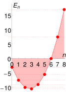
Figure 1: Spectrum and energy eigenstates. (a), the first nine energy eigenvalues of the harmonic oscillator $h_{n}=n+\frac{1}{2}$ for $n=0,1,2,...,8$ are mapped via the polynomial ${\cal P}(\xi)=\xi^{2}-\frac{13}{2}\xi$ to $E_{n}={\cal P}(h_{n})$. This map changes the order of the values $E_{n}$ such that the state with index $n=3$ has the lowest eigenenergy $E_{3}=-\frac{21}{2}$. (b), the wave functions, with their ordinate off-set by $E_{n}$, are displayed together with the cross-section ${\cal P}(\frac{1}{2}x^{2})={\cal H}(x,0)$ of the hamiltonian.

II.2 Dialling up the spectrum

We now show that we can dial up an arbitrary real point spectrum for the $N$ first energy eigenstates of $\hat{\cal H}$. Note, by ‘first’ we mean the entries of the column-vector $\mbox{\boldmath${E}$}_{(N)}=[E_{0},E_{1},...,E_{N-1}]^{\top}$ of Eq. (3). Because of the reordering, these are in general not the lowest lying energy values.

Rewriting Eq. (2) in a suitable matrix form is achieved by casting the energy values of $\hat{h}^{j}$ into the form of a square $N\times N$ ‘energy-matrix’ $[\mbox{\boldmath${\epsilon}$}_{(N)}]_{n,j}=(h_{n})^{j}$. The coefficient column-vector $\mbox{\boldmath${a}$}_{(N)}=[a_{1},a_{2},...,a_{N}]^{\top}$ then, according to Eq. (2), obeys $\mbox{\boldmath${E}$}_{(N)}=\mbox{\boldmath${\epsilon}$}_{(N)}\cdot\mbox{\boldmath${a}$}_{(N)}$ where the dot stands for matrix multiplication.

For instance, $\mbox{\boldmath${\epsilon}$}_{(5)}$ has the form

$$\mbox{\boldmath${\epsilon}$}_{(5)}=\begin{bmatrix}\frac{1}{2}&\frac{1}{4}&\frac{1}{8}&\frac{1}{16}&\frac{1}{32}\\[4.0pt] \frac{3}{2}&\frac{9}{4}&\frac{27}{8}&\frac{81}{16}&\frac{243}{32}\\[4.0pt] \frac{5}{2}&\frac{25}{4}&\frac{125}{8}&\frac{625}{16}&\frac{3125}{32}\\[4.0pt] \frac{7}{2}&\frac{49}{4}&\frac{343}{8}&\frac{2401}{16}&\frac{16807}{32}\\[4.0pt] \frac{9}{2}&\frac{81}{4}&\frac{729}{8}&\frac{6561}{16}&\frac{59049}{32}\\ \end{bmatrix}.$$ (5)

The determinant $|\mbox{\boldmath${\epsilon}$}_{(N)}|=\prod_{g=1}^{N-1}[g!(2g+1)]/2^{N}$ is non-zero, hence, $\mbox{\boldmath${\epsilon}$}_{(N)}$ can always be inverted: any column vector $\mbox{\boldmath${E}$}_{(N)}$ uniquely specifies a coefficient vector $\mbox{\boldmath${a}$}_{(N)}$ where

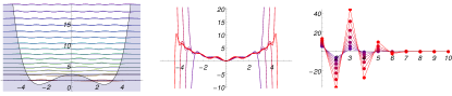
Figure 2: Quantum mechanical potential $V(x)$, its analogue $\hat{\cal H}$ for varying orders and the associated expansion coefficients. (a), for the hamiltonian $\hat{H}$ its potential $V(x)=3-(2x^{2})/3+x^{4}/27+x^{6}/729$ is shown with its energy levels. (b), $\hat{H}$ is mapped to equivalent hamiltonian’s $\hat{\cal H}_{(N)}$ of progressively increasing order ranging from $N=4$ to 10. The increase in order is reflected in the colour coding (blue for $N$=4 to red for $N$=10) of the associated plots of the cross-sections ${\cal P}_{(N)}(\frac{1}{2}x^{2})={\cal H}_{(N)}(x,0)$. We notice that the expansion coefficients ${\mbox{\boldmath${a}$}}_{(N)}$ do not settle, instead, across the board, they increase in magnitude with increasing $N$: see (c) [employing the same color coding as (b)]. Moreover, the expansion coefficients $a_{j}$ alternate in sign, this implies that for the potential $V(x)$, displayed in (b), ${\cal H}_{(N)}(r)$ is negative (open downward) for large values of $r=\sqrt{x^{2}+p^{2}}$ if $N$ is even, and positive (closed) for odd $N$.

$$\mbox{\boldmath${a}$}_{(N)}=\mbox{\boldmath${\epsilon}$}^{-1}_{(N)}\cdot\mbox{\boldmath${E}$}_{(N)}\;$$ (6)

and thus $\mbox{\boldmath${a}$}_{(N)}$ specifies a formal hamiltonian $\hat{\cal H}_{(N)}$ for which the first $N$ eigenfunctions $|\phi_{n}\rangle$ have energies $\mbox{\boldmath${E}$}_{(N)}$.

As mentioned before, this observation implies that $\hat{\cal H}$ can be formed such that any level is randomly assigned any real energy value: $\langle\phi_{n}|\hat{\cal H}|\phi_{n}\rangle=E_{n}$.

However, in quantum mechanical systems we expect the Sturm-Liouville level ordering rule to be obeyed.

In Subsection IV.1 we will find that in our construction violations of the Sturm-Liouville level ordering rule arise spontaneously but, fortunately, when we restrict the order of ${\cal P}_{(N)}$ to either even or odd values of $N$ (depending on the system $\hat{H}$ considered) this irritating ordering violation is absent.

In other words: if for a given potential $V(x)$ the mapping of $H$ onto ${\cal H}_{(N)}$ does not reproduce the lowest $N$ values of $\mbox{\boldmath${E}$}_{(N)}$, then a mapping onto ${\cal H}_{(N+1)}$ will.

Despite the fact that $H$ and the formal hamiltonian ${\cal H}_{(N)}$ share parts of their energy spectrum, $V(x)$ and ${\cal H}_{(N)}(x,0)$ do not have any obvious functional relationship, see Fig. 2. This observation is reinforced by the fact that the formal hamiltonian ${\cal H}_{(N)}$ is invariant under parity transformations whereas $\hat{H}$ in general is not.

One is also free to generalise our approach, for example, by assigning energy values to only some eigenfunctions $\phi_{n}$. To this end one can strip out the $m$-th entry in ${E}$ together with the $m$-th row in ${\epsilon}$ thus removing an assignment for an ‘unwanted’ state $\phi_{m}$ [whose value would still be assigned implicitly through Eq. (3)]. One then also has to strip out one column of ${\epsilon}$ (together with the associated entry in ${a}$) to keep ${\epsilon}$ invertible. This column could, e.g., be the last ($N$-th) column in which case the order of polynomial $\cal P$ would be reduced by one.

II.3 Shifting the ground state energy $E_{0}$

The expansion coefficients ${a}$ depend on the value of $E_{0}$. We cannot shift the harmonic oscillator’s spectrum such that its ground state energy $h_{0}=0$ since that would render $|\mbox{\boldmath${\epsilon}$}|=0$ making $\mbox{\boldmath${\epsilon}$}^{-1}$ in Eq. (6) ill-defined. We will therefore from now on, for definiteness, set $E_{0}=0$: for further justification see Fig. 3.

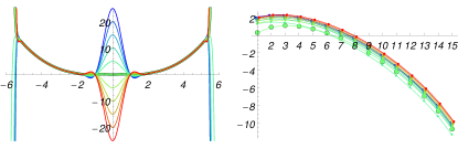
Figure 3: Expansion coefficients vary with shift of energy. The ground state energy $E_{0}$ for $\hat{H}$ with $V(x)=1-(2x^{2})/9+x^{4}/81+x^{6}/729$ is shifted (together with the rest of the energy spectrum) from -25 (red color) via 0 (green color, which is highlighted) to +25 (blue color). The associated curves for ${\cal H}(x,0)$ are shown in panel (a) and the magnitude of the expansion coefficients $\log_{10}|a_{j}|,j=1,...,15$ in panel (b). One can see that the expansion coefficients tend to be small in magnitude for small energy offsets, in other words, setting $E_{0}=0$ (green lines) is a reasonable choice.

III Computational implementation of $\hat{\cal H}$ and stability considerations

III.1 Using exact fractions

Since we could not determine the general explicit form of $\mbox{\boldmath${\epsilon}$}^{-1}$ in Eq. (6) we let a program determine it, in terms of exact fractions, to avoid numerical instabilities associated with approximations of $\mbox{\boldmath${\epsilon}$}^{-1}$. With modern computer algebra systems it is feasible to do so, in seconds, for $N$-values of order $10^{3}$.

For the sake of numerical stability we found that the energy eigenvalues of $\hat{H}$, which are used as input values, also have to be formally written in analytical form, namely as fractions (e.g., $E_{5}=10.453$ should be written as $E_{5}=10453/1000$). Then, even for fairly large values ${\cal O}(N)\approx 10^{3}$ can the analogue hamiltonian $\hat{\cal H}_{(N)}$ be constructed safely using Eq. (6). The associated high order polynomial function ${\cal P}(x,p)$ is of order $2N$ in $x$ and $p$ and therefore becomes numerically unmanageable for moderate values ${\cal O}(N)\approx 10^{2}$, fortunately that does not affect the stability of the underlying scheme encapsulated by Eq. (6).

III.2 The coefficients do not settle down

The expansion coefficients ${\mbox{\boldmath${a}$}}_{(N)}$ for a chosen quantum mechanical hamiltonian $H$ do not settle down with increasing order $N$ of the number of mapped energy values ${\mbox{\boldmath${E}$}}_{(N)}$, see Fig. 2 (c); they alternate and increase in value with $N$. The underlying reason for this behaviour is the fact that, with every added order $j$ of $\hat{h}^{j}$, momentum terms of order $\hat{p}^{2j}$ are added. Their presence leads to so much ‘kinetic energy’ added with every order that even infinite-box potentials display oscillations of the coefficients $a_{j}$.

Therefore, typically, $\lim_{N\rightarrow\infty}{\cal H}_{(N)}$ does not exist.

IV Smooth deformations of the potential and its effect on ${\cal H}_{(N)}$

IV.1 Even versus odd number of levels

In the mapping of $\hat{H}$ to $\hat{\cal H}_{(N)}$ we observed that for the fixed potential portrayed in Fig. 2 (a) the expansion order $N$ should be odd to avoid a downward open potential that violates the Sturm-Liouville level ordering rule, see Fig. 2 (b). In general, a fixed potential $V(x)$ requires either even or odd expansion orders $N$ to achieve this. This observation of an even-odd-$N$ bias is generic, since the oscillations of the coefficients $a_{j}$, as seen in Fig. 2 (c), is typical.

The observation of such an ‘even-odd bias’ in the desirable orders of the expansion for ${\cal H}_{(N)}$ raises the question whether one can use this bias to devise a criterion for grouping potentials into separate, inequivalent classes.

IV.2 Deformation from single well to deep double well potential

In the case of a continuous transition of single well to double well potentials, as sketched in Fig. 4, such an even-odd transition occurs once. In this case we do not, for instance, witness a back-and-forth switching between even-odd and odd-even biases with, say, every addition of the next higher eigenstate to the tunnelling regime.

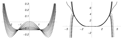
Figure 4: Expansion order bias switch in deformed potentials. Panel (a) displays potentials $V(x)=V_{0}\left[1-(2x^{2})/9+x^{4}/81\right]+x^{6}/729-E_{0}$ where $V_{0}$ is incremented from 0 to 0.5 in ten equal steps of size $0.05$. This leads to a transition from single to double well potential where the groundstate (at shifted energy $\tilde{E}_{0}=0$) just starts to tunnel. Panel (b) displays the associated formal hamiltonians ${\cal H}_{(6)}$ and shows that an even to odd transition for the desirable expansion order $N$ occurs. For more details see main text.

IV.3 Multi-well systems

Instead of deforming the potentials such that they form increasingly deeper wells, as considered in Fig. 4, we now consider systems with an increase in the number of adjacent wells, see Fig. 5.

We map this to a sixth-order formal hamiltonian $\hat{\cal H}_{(6)}$ and observe even-odd-$N$ bias transitions whenever another well is added.

Similarly to our finding reported in Fig. 4, an increase in the barrier height between adjacent wells does, however, not affect the observed even-odd-$N$ bias:

The even-odd-$N$ biases can be used to discriminate between different numbers of wells in multi-well potentials but not between the strength of the barriers between the wells.

The question whether this can be a useful criterion to sensitively discriminate between different types of hamiltonians in other contexts remains open.

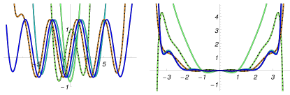
Figure 5: Expansion order bias in multi-well systems. Panel (a) displays potentials for which the number of adjacent wells increases from 1 to 5. Panel (b) displays the associated formal hamiltonians ${\cal H}_{(6)}$, which are depicted by the same coloring of the graph as in panel (a). This shows that a transition in the even-odd-$N$ bias for the desirable expansion order $N$ occurs whenever another well is added: curves are dashed when ${\cal H}_{(6)}(x,0)<0$ for large values of $x$.

V Phase space behaviour

The evolution of the Wigner’s phase space distribution function in quantum phase space is governed by the continuity equation $\frac{\partial W}{\partial t}=-\mbox{\boldmath${\nabla}$}\cdot\mbox{\boldmath${J}$}$, where ${J}$ is Wigner’s current Oliva et al. (2017).

Hamiltonians of the form $\hat{\cal H}={\cal P}(\hat{h})$ have special dynamical features: their phase space current follows circles concentric to the phase space origin; for a proof see the Appendix of Ref. Oliva and Steuernagel (2019). In other words, their phase space current is tangential to the system’s energy contours.

We now show that such a special alignment cannot be constructed for quantum mechanical systems with anharmonic potentials $V(x)$.

In reference Oliva et al. (2017) it was shown that anharmonic systems exhibit singularities of the associated phase space velocity field. This precludes the possibility of mapping them to system whose dynamics can be described by the Poisson-bracket of classical physics Kakofengitis et al. (2017), but directional alignment of ${J}$ with the energy contours is not ruled out.

For a contradiction, assume that the desired directional alignment is possible for anharmonic quantum mechanical systems when using a correction to the current field ${\tilde{J}}$, where $\mbox{\boldmath${\nabla}$}\cdot\mbox{\boldmath${\tilde{J}}$}=0$, to not affect the dynamics.

Per assumption $\mbox{\boldmath${J}$}+\mbox{\boldmath${\tilde{J}}$}$ is aligned with the classical hamiltonian flow in phase space and therefore shares its stagnation points. But at a stagnation point $\partial_{t}W=0$, yet we know that quantum and classical phase space current stagnation points do not in general coincide Kakofengitis and Steuernagel (2017): anharmonic quantum hamiltonians can therefore not feature phase space current fields aligned with their energy contours, unless they are of form $\hat{\cal H}$.

VI Mapped states

In this work we implicitly considered the diagonalization of a wide variety of hamiltonians $H$ and their subsequent mapping to generic systems of the form ${\cal H}$. The diagonalization of a quantum hamiltonian is not a smooth transformation.

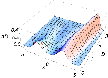
Figure 6: Mapped ‘coherent states’. Using Glauber coherent state coefficients for the energy eigenstates $\psi_{j}(x)$ of potential $V(x)=3-(2x^{2})/3+x^{4}/27+x^{6}/729$, see Fig. 2 (a), the mapped ‘coherent states’ $\Psi(x,D)=\exp[-|D|^{2}/2]\frac{D^{j}}{\sqrt{j!}}\;\psi_{j}(x)$, displaced by $D$, are formed. Their non-Gaussian shape illustrates that the mapping between $\hat{H}$ and $\hat{\cal H}$ distorts features of wave functions.

It is therefore of some interest to get a feeling for the distortions a state suffers when mapping between hamiltonians $H$ and ${\cal H}$. For illustration we consider the distortions a gaussian Glauber-coherent state of system $\hat{\cal H}$ suffers, as a function of displacement from the origin, when mapped to a double well system, see Fig. 6.

VII Conclusions

We have identified a class of formal hamiltonians $\hat{\cal H}$ of one-dimensional continuous quantum systems that feature energy point spectra which can be dialled up at will.

Owing to the occurrence of high orders in momenta, the eigenfunctions of $\hat{\cal H}$ for these point spectra can be out of order with respect to the number of nodes associated with level numbers (violation of Sturm-Liouville monotonic energy-level ordering rule).

We can however restrict the formal hamiltonians $\hat{\cal H}_{(N)}$ to even or odd expansion order $N$ to enforce monotonic level ordering.

Our observations raise the question whether the construction of formal hamiltonians $\hat{\cal H}$ provides a useful tool to universally represent and treat ‘all discrete spectrum quantum systems’ on an equal footing.

Investigation of the generalization of this approach to interacting multiparticle systems appears warranted.