Robust Optimal-Complexity Multilevel ILU for
Predominantly Symmetric Systems

Abstract

Incomplete factorization is a powerful preconditioner for Krylov subspace methods for solving large-scale sparse linear systems. Existing incomplete factorization techniques, including incomplete Cholesky and incomplete LU factorizations, are typically designed for symmetric or nonsymmetric matrices. For some numerical discretizations of partial differential equations, the linear systems are often nonsymmetric but predominantly symmetric, in that they have a large symmetric block. In this work, we propose a multilevel incomplete LU factorization technique, called PS-MILU, which can take advantage of predominant symmetry to reduce the factorization time by up to half. PS-MILU delivers robustness for ill-conditioned linear systems by utilizing diagonal pivoting and deferred factorization. We take special care in its data structures and its updating and pivoting steps to ensure optimal time complexity in input size under some reasonable assumptions. We present numerical results with PS-MILU as a preconditioner for GMRES for a collection of predominantly symmetric linear systems from numerical PDEs with unstructured and structured meshes in 2D and 3D, and show that PS-MILU can speed up factorization by about a factor of 1.6 for most systems. In addition, we compare PS-MILU against the multilevel ILU in ILUPACK and the supernodal ILU in SuperLU to demonstrate its robustness and lower time complexity
Keywords: incomplete LU factorization; multilevel methods; Krylov subspace methods; robust preconditioners; linear-time algorithms; predominantly symmetric systems

1 Introduction

Preconditioned Krylov subspace (KSP) methods are widely used for solving sparse linear systems, especially those arising from numerical discretizations of partial differential equations (PDEs). These methods typically require some robust and efficient preconditioners to be effective, especially for large-scale problems. Incomplete factorization techniques, including incomplete LU factorization with pivoting for nonsymmetric systems or incomplete Cholesky factorization for symmetric and positive definite (SPD) systems, are among the most robust preconditioners, and some of their variants are often quite efficient for linear systems arising from PDE discretizations. In practice, some linear systems are often nonsymmetric but have a symmetric block, and it is worth exploring this partial symmetry to improve the robustness and efficiency of the incomplete factorizations. Without loss of generality, we assume the matrix is real and the symmetric part is the leading block; i.e., the matrix $\boldsymbol{A}\in\mathbb{R}^{n\times n}$ has the form

$$\boldsymbol{A}=\begin{bmatrix}\boldsymbol{B}&\boldsymbol{F}\\ \boldsymbol{E}&\boldsymbol{C}\end{bmatrix},$$ (1)

where $\boldsymbol{B}\in\mathbb{R}^{n_{1}\times n_{1}}$ symmetric and $\boldsymbol{E}\neq\boldsymbol{F}^{T}$. Note that form (1) includes symmetric and nonsymmetric matrices as special cases, for which $\boldsymbol{C}$ and $\boldsymbol{B}$ are empty, respectively. We are particularly interested in the case where the size of $\boldsymbol{B}$ dominates that of $\boldsymbol{C}$, and we refer to such systems as predominantly symmetric. These systems may arise from PDE discretizations. For example, for the Poisson equation with Dirichlet boundary conditions, if the Dirichlet nodes are not eliminated from the system, then we have $\boldsymbol{C}=\boldsymbol{I}$, $\boldsymbol{E}=\boldsymbol{0}$, and $\boldsymbol{F}\neq\boldsymbol{0}$. Another example is the finite difference methods for the Poisson equation with Neumann boundary conditions on a structured mesh: If centered difference is used in the interior and one-sided difference is used for Neumann boundary conditions, then we obtain a predominantly symmetric system, where the rows in $\boldsymbol{B}$ correspond to the interior nodes and those in $\boldsymbol{C}$ correspond to the Neumann nodes. Similarly, for some variants of finite difference methods, such as embedded boundary and immersed boundary methods for parabolic or elliptic problems, the matrix block corresponding to the interior nodes may be symmetric but that corresponding to near-boundary nodes is in general nonsymmetric. Other examples include finite element methods with a high-order treatment of Neumann boundary conditions over curved domains, which modify the rows in the stiffness matrix corresponding to Neumann nodes instead of simply substituting the boundary conditions to the right-hand side vector; see e.g. [5]. In all these examples, due to the surface-to-volume ratio, the size of $\boldsymbol{C}$ is much smaller than that of $\boldsymbol{B}$.

Given a predominantly symmetric matrix in form (1), it is conceivable that one would like to take advantage of the symmetry in $\boldsymbol{B}$ to reduce the factorization time, especially if the size of $\boldsymbol{B}$ dominates that of $\boldsymbol{C}$. To the best of our knowledge, there was no incomplete factorization technique in the literature that can take advantage of this predominant symmetry. The lack of such a method is probably because most incomplete factorization techniques are based on variants of LU factorization with or without column pivoting for nonsymmetric systems or Cholesky factorization for SPD systems. Since LU with column pivoting would destroy the symmetry, whereas LU without pivoting is unstable, there is no known stable LU factorization techniques for predominantly symmetric systems. As a result, it is a challenging task to develop an incomplete ILU algorithm for predominantly symmetric systems, and it requires a drastically different approach than traditional factorization techniques. Note that the form (1) shares some similarity with KKT systems, which often require special solvers; see [3] for an extensive survey. However, (1) is different from KKT systems in that $\boldsymbol{E}\neq\boldsymbol{F}^{T}$ and $\boldsymbol{C}$ is typically nonzero in (1). Although a preconditioner for (1) may be applied to KKT systems, the converse is in general not true.

In this paper, we propose an incomplete ILU technique, referred to as PS-MILU, for predominantly symmetric systems, which will provide a robust, efficient, and unified factorization algorithm for symmetric and nonsymmetric systems. We develop this method based on the following key ideas. First, we introduce a modified version of the Crout update procedure in [28] to support symmetric LDL${}^{\text{T}}$ and nonsymmetric LDU factorizations with diagonal pivoting. Second, to improve robustness, we adopt the framework of multilevel ILU factorization [10] to defer the factorizations of rows and columns that would cause the norms of $\boldsymbol{L}^{-1}$ and $\boldsymbol{U}^{-1}$ to grow rapidly. Third, to achieve efficiency, we limit the number of nonzeros in the approximate factors to be within a constant factor of those in the input, and develop data structures to ensure optimal time complexity of the overall algorithm. In particular, we ensure that the cost of updating the nonzeros in the $\boldsymbol{L}$ and $\boldsymbol{U}$ factors is linear, assuming the number of nonzeros per row and per column is bounded by a constant, and its cost dominates all the other steps, including pivoting, sorting, dropping, and computing of the Schur complement, etc. As a result, PS-MILU delivers a robust and optimal-complexity method for most linear systems from PDE discretizations. Furthermore, it can speed up the factorization by up to a factor of two for predominantly symmetric systems. We present numerical results with PS-MILU as a preconditioner for GMRES for a collection of linear systems from numerical PDEs with unstructured and structured meshes in 2D and 3D. In addition, we compare PS-MILU against the multilevel ILU with diagonal pivoting in ILUPACK [11] and the supernodal ILU with column pivoting in SuperLU [30]. Our numerical results show that PS-MILU scales better than both ILUPACK and SuperLU, while delivering comparable robustness.

The remainder of the paper is organized as follows. In Section 2, we review some background knowledge on incomplete ILU factorization and its variants. In Section 3, we describe the components of the proposed multilevel ILU for predominantly symmetric systems. In Section 4, we present some implementation details of the algorithm, with a focus on the data structure, updating and pivoting, and the complexity analysis. In Section 5, we present some numerical results with PS-MILU as a preconditioner for GMRES and compare its performance with other techniques. Finally, Section 6 concludes the paper with a discussion of future work.

2 Background

The technique proposed in this work is based on multilevel ILU factorization, which is one of the most effective preconditioner for Krylov subspace methods. Multilevel ILU is a sophisticated variant of incomplete LU factorization. In [24], we compared multilevel ILU against some other preconditioners (including SOR, ILU with and without thresholding or pivoting [32], BoomerAMG [38] and smoothed-aggregation AMG [21]) for several Krylov subspace methods (including GMRES [36], BiCGSTAB [41], TFQMR [20], and QMRCGSTAB [13]). It was shown that although multigrid methods are often the most efficient preconditioners when applicable, thanks to its nearly linear scaling, incomplete LU techniques are more robust for ill-conditioned systems. Among the incomplete LU techniques, multilevel ILU delivers the best balance between robustness and efficiency. In this section, we give a brief overview of incomplete LU factorization. We refer readers to [14] for a survey of incomplete factorization techniques up to 1990s and refer readers to [24] for a recent comparison of ILU with other preconditioners for nonsymmetric systems.

At a high-level, incomplete LU (or ILU) without pivoting performs an approximate factorization

$$\boldsymbol{P}^{T}\boldsymbol{A}\boldsymbol{Q}\approx\boldsymbol{L}\boldsymbol{U},$$ (2)

where $\boldsymbol{L}$ and $\boldsymbol{U}$ are far sparser than their corresponding factors in the complete LU factorization of $\boldsymbol{A}$ after some row and column reordering. Let $\boldsymbol{M}=\boldsymbol{L}\boldsymbol{U}$, so that $\boldsymbol{P}\boldsymbol{M}\boldsymbol{Q}^{T}$ is a preconditioner of $\boldsymbol{A}$, or equivalently $\boldsymbol{M}$ is a preconditioner of $\boldsymbol{P}^{T}\boldsymbol{A}\boldsymbol{Q}$. In general, $\boldsymbol{M}$ is a good preconditioner if the eigenvalues of $\boldsymbol{P}^{T}\boldsymbol{A}\boldsymbol{Q}\boldsymbol{M}$ are well clustered. Given a linear system $\boldsymbol{A}\boldsymbol{x}=\boldsymbol{b}$, if right-preconditioning is used, which is typically preferred over left-preconditioning [24], the system is then solved by first solving

$$\boldsymbol{A}\left(\boldsymbol{P}\boldsymbol{M}\boldsymbol{Q}^{T}\right)^{-1}\boldsymbol{y}=\boldsymbol{b},$$ (3)

and then $\boldsymbol{x}=\left(\boldsymbol{P}\boldsymbol{M}\boldsymbol{Q}^{T}\right)^{-1}\boldsymbol{y}=\boldsymbol{Q}\boldsymbol{U}^{-1}\boldsymbol{L}^{-1}\boldsymbol{P}^{T}\boldsymbol{y}$. This type of preconditioner was first used by Simon [37] for SPD systems, for which incomplete LU reduces to incomplete Cholesky factorization with symmetric reordering, i.e., $\boldsymbol{P}^{T}\boldsymbol{A}\boldsymbol{P}\approx\boldsymbol{R}^{T}\boldsymbol{R}$.

In its simplest form, ILU does not involve any pivoting, and $\boldsymbol{L}$ and $\boldsymbol{U}$ preserve the sparsity patterns of the lower and upper triangular parts of $\boldsymbol{A}$, respectively. This approach is often referred to as ILU0 or ILU(0). Unfortunately, it is typically ineffective and often fails in practice. For linear systems arising from elliptic PDE, a simple modification, first used in [19] and [26], is to modify the diagonal entries to compensate the discarded entries, for example by adding up all the entries that have been dropped and then subtracting the sum from the corresponding diagonal entry of $\boldsymbol{U}$. This is known as modified ILU [34]. A more general approach is to allow fills, a.k.a. fill-ins, which are new nonzeros in the $\boldsymbol{L}$ and $\boldsymbol{U}$ factors at the zeros in $\boldsymbol{A}$. Traditionally, the fills are introduced based on their levels in the elimination tree or based on the magnitude of numerical values. The former leads to the so-called ILU($k$), which zeros out all the fills of level $k+1$ or higher in the elimination tree. The combination of the two is known as ILU with dual thresholding (ILUT) [32]. Most implementations of ILU, such as those in PETSc [2], hypre [38], and the fine-grained parallel ILU algorithm [15], use some variants of ILUT, and they may also allow the user to control the number of fills in each row.

Because ILUT does not involve pivoting, its effectiveness is still limited. It often fails in practice for ill-conditioned problems or for KKT-like systems. To improve its robustness, partial pivoting can be added into ILUT, leading to the so-called ILUTP [34]. The ILU implementations in MATLAB [39], SPARSKIT [33], and SuperLU [30], for example, are based on ILUTP. However, ILUTP suffers from a major drawback: in general, a small drop tolerance is needed for ILUTP for robustness, but a large drop tolerance is needed to avoid rapid growth in the number of fills. As a result, parameter tuning for ILUTP is a difficult, and sometimes even impossible, task. Often, the number of fills in ILUTP grows nearly quadratically for PDE problems as the problem sizes grow, so it is impractical to use ILUTP for very large-scale problems.

The issues of non-robustness of ILUT and poor-scaling of ILUTP are mitigated by multilevel ILU, or MILU for short. Unlike ILUTP, MILU uses diagonal pivoting instead of partial pivoting with a deferred factorization for “problematic” rows and columns. More specifically, if a particular row or column would lead to a large $\left\|\boldsymbol{L}^{-1}\right\|_{\infty}$ or $\left\|\boldsymbol{U}^{-1}\right\|_{1}$, which are estimated incrementally, then the row and its corresponding column will be permuted to the lower-right corner of $\boldsymbol{A}$ to be factorized more robustly in the next level [7, 9]. Specifically, let $\boldsymbol{P}$ and $\boldsymbol{Q}$ denote the permutation matrices due to diagonal pivoting and some reordering. A preconditioner $\boldsymbol{M}$ corresponding to the permuted matrix $\boldsymbol{P}^{T}\boldsymbol{A}\boldsymbol{Q}$ can be constructed via the approximation

$$\boldsymbol{P}^{T}\boldsymbol{A}\boldsymbol{Q}=\begin{bmatrix}\hat{\boldsymbol{B}}&\hat{\boldsymbol{F}}\\ \hat{\boldsymbol{E}}&\hat{\boldsymbol{C}}\end{bmatrix}\approx\hat{\boldsymbol{M}}=\begin{bmatrix}\boldsymbol{I}&0\\ \hat{\boldsymbol{E}}\tilde{\boldsymbol{B}}^{-1}&\boldsymbol{I}\end{bmatrix}\begin{bmatrix}\tilde{\boldsymbol{B}}&0\\ 0&\boldsymbol{S}_{C}\end{bmatrix}\begin{bmatrix}\boldsymbol{I}&\tilde{\boldsymbol{B}}^{-1}\hat{\boldsymbol{F}}\\ 0&\boldsymbol{I}\end{bmatrix},$$ (4)

where $\tilde{\boldsymbol{B}}$ approximates $\hat{\boldsymbol{B}}$ via incomplete factorization, i.e., $\hat{\boldsymbol{B}}\approx\tilde{\boldsymbol{B}}=\boldsymbol{L}\boldsymbol{U}$; $\hat{\boldsymbol{C}}$, $\hat{\boldsymbol{E}}$ and $\hat{\boldsymbol{F}}$ are composed of the deferred rows and columns; $\boldsymbol{S}_{C}$ is its Schur complement. Here, $\hat{\boldsymbol{B}}$ is in general nonsymmetric, unlike $\boldsymbol{B}$ in (1). Note that

$$\hat{\boldsymbol{M}}^{-1}=\begin{bmatrix}\tilde{\boldsymbol{B}}^{-1}&\boldsymbol{0}\\ \boldsymbol{0}&\boldsymbol{0}\end{bmatrix}+\begin{bmatrix}-\tilde{\boldsymbol{B}}^{-1}\hat{\boldsymbol{F}}\\ \boldsymbol{I}\end{bmatrix}\boldsymbol{S}_{C}^{-1}\begin{bmatrix}-\hat{\boldsymbol{E}}\tilde{\boldsymbol{B}}^{-1}&\boldsymbol{I}\end{bmatrix}.$$ (5)

Approximating the inverse of $\boldsymbol{S}_{C}$ by the same construction recursively, we obtain a “multilevel” structure. Let $\left(\boldsymbol{P}_{S}^{T}\boldsymbol{S}_{C}\boldsymbol{Q}_{S}\right)^{-1}$ be approximated by $\boldsymbol{Q}_{S}^{T}\tilde{\boldsymbol{S}}_{C}^{-1}\boldsymbol{P}_{S}$, where $\boldsymbol{P}_{S}$ and $\boldsymbol{Q}_{S}$ denote the permutation matrices due to diagonal pivoting and reordering on $\boldsymbol{S}_{C}$. The multilevel preconditioner $\boldsymbol{M}$ is defined by

$$\boldsymbol{M}^{-1}=\begin{bmatrix}\tilde{\boldsymbol{B}}^{-1}&\boldsymbol{0}\\ \boldsymbol{0}&\boldsymbol{0}\end{bmatrix}+\begin{bmatrix}-\tilde{\boldsymbol{B}}^{-1}\hat{\boldsymbol{F}}\\ \boldsymbol{I}\end{bmatrix}\tilde{\boldsymbol{S}}_{C}^{-1}\begin{bmatrix}-\hat{\boldsymbol{E}}\tilde{\boldsymbol{B}}^{-1}&\boldsymbol{I}\end{bmatrix}.$$ (6)

Compared to ILUT, MILU is shown to be more robust, thanks to its diagonal pivoting and deferred factorization. Compared to ILUTP, MILU significantly reduces the number of fills by avoiding partial pivoting. In addition, the estimated inverse norm in MILU is also used in the dropping criteria to further improve robustness. A robust serial implementation of MILU is available in ILUPACK [10, 11].

For virtually all ILU techniques, some preprocessing steps, including scaling (commonly referred to as matching) and reordering, can help improve their efficiency and robustness [18, 4]. Scaling aims to scale the rows and columns of the matrix such that the diagonal entries have magnitude $1$ and the off-diagonal entries have magnitude no greater $1$. To this end, the matrix may need to be permuted using a graph matching algorithm, and hence this procedure is often referred to as matching. A commonly used scaling procedure is the MC64 routine in the HSL library [18], which is based on the maximum weighted bipartite matching algorithm in [31]. MC64 supports both symmetric and nonsymmetric matrices. For symmetric matrices, permutation is done symmetrically to rows and columns, and hence it may be impossible to make all the diagonal entries to have magnitude $1$. In such cases, the matching algorithm may need to construct $2\times 2$ diagonal blocks whose off-diagonal entries have magnitude $1$. After matching, one may perform reordering to further reduce fills during factorization. The popular reordering techniques including approximate minimum degree (AMD) [1], nested dissection (ND) [22], etc., which are commonly used in sparse LU or Cholesky factorizations. To preserve the effect of scaling, reordering should be performed symmetrically. For nonsymmetric matrices, this can be done by applying the symmetric AMD on $\boldsymbol{A}+\boldsymbol{A}^{T}$. For symmetric matrices, a robust reordering algorithm would need to be performed on the block matrix to preserve the $2\times 2$ diagonal blocks. In our experiments, MILU with MC64 matching/scaling and symmetric AMD reordering tends to deliver very good results, which will be the basis of this work.

3 Predominantly Symmetric Multilevel Incomplete LU-Factorization

Our proposed method, PS-MILU, aims to exploit the symmetry in (1) to provide a unified algorithm for symmetric and nonsymmetric matrices and to improve efficiency for predominantly symmetric matrices. To this end, we consider incomplete LDU factorizations, where the approximate $\boldsymbol{L}$ and $\boldsymbol{U}$ factors are unit lower and upper triangular matrices, respectively. For symmetric matrices, $\boldsymbol{U}=\boldsymbol{L}^{T}$, so LDU factorization reduces to LDL${}^{\text{T}}$ factorization. We use a multilevel framework with matching, scaling, reordering, and diagonal pivoting at each level, which will preserve the symmetry of the leading symmetric block.

Figure 1 shows the overall flowchart of our algorithm. The algorithm takes the input matrix in the form (1). If the leading block $\boldsymbol{B}$ is symmetric, then we will use incomplete LDL${}^{\text{T}}$ factorization with symmetric matching and reordering. Note that for best efficiency, the user may need to permute the matrix beforehand so that the leading symmetric block $\boldsymbol{B}$ is as large as possible. In the context of PDE discretizations, this typically involves putting the interior nodes before the boundary nodes in the matrix. The algorithm uses diagonal pivoting to push “problematic” rows and columns in $\boldsymbol{B}$ to the lower-right corner, which are then merged into $\boldsymbol{C}$, $\boldsymbol{E}$ and $\boldsymbol{F}$, whose corresponding Schur complement $\boldsymbol{S}_{C}$ is then factorized recursively. The recursion stops if the Schur complement is small or dense enough.

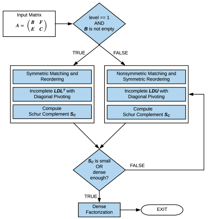
Figure 1: The overall workflow of PS-MILU.

Overall, our algorithm has five main components:

1. preprocessing, including MC64 matching and AMD reordering for improving diagonal dominance and reducing fills;

2. modified Crout incomplete factorization, namely, incomplete symmetric LDL${}^{\text{T}}$ and nonsymmetric LDU factorizations, which adapt the Crout update of $\boldsymbol{L}$ and $\boldsymbol{U}$ to support early update of $\boldsymbol{D}$ for diagonal pivoting;

3. diagonal pivoting, for controlling the growth of $\left\|\boldsymbol{L}^{-1}\right\|_{\infty}$ and $\left\|\boldsymbol{U}^{-1}\right\|_{1}$;

4. inverse-based thresholding, which controls the dropping in $\boldsymbol{L}$ and $\boldsymbol{U}$ to control the growth of the inverse norm;

5. hybrid Schur complement, which modifies the Schur complement by adaptively adding a correction term to compensate the leading error term associated with droppings in the current level.

In the following subsections, we will describe each of these components in more detail.

3.1 Preprocessing for PS-MILU

In PS-MILU, we apply matching, scaling, and reordering at each level before factorization. We use the HSL library subroutine MC64 [18] followed by symmetric AMD [1] for these purposes.

Consider the input matrix $\boldsymbol{A}$ in (1), and assume the leading symmetric block $\boldsymbol{B}$ is not empty. We apply symmetric MC64 on $\boldsymbol{B}$, followed by symmetric AMD. Let

$$\boldsymbol{A}_{1}=\boldsymbol{P}_{1}^{T}\boldsymbol{D}_{1}\boldsymbol{B}\boldsymbol{D}_{1}\boldsymbol{P}_{1},$$ (7)

where $\boldsymbol{D}_{1}$ and $\boldsymbol{P}_{1}$ are the scaling and permutation matrices, respectively. For now, let us assume that symmetric matching is successful, so that the diagonals of $\boldsymbol{A}_{1}$ are all ones. Let $\hat{\boldsymbol{P}}=\begin{bmatrix}\boldsymbol{P}_{1}\\ &\boldsymbol{I}\end{bmatrix}$ and $\hat{\boldsymbol{D}}=\begin{bmatrix}\boldsymbol{D}_{1}\\ &\boldsymbol{I}\end{bmatrix}$, where $\boldsymbol{I}$ has the same dimension as $\boldsymbol{C}$. Then, we obtain

$$\hat{\boldsymbol{A}}=\hat{\boldsymbol{P}}^{T}\hat{\boldsymbol{D}}\boldsymbol{A}\hat{\boldsymbol{D}}\hat{\boldsymbol{P}}.$$ (8)

Figure 2 shows the sparsity patterns of an example predominantly symmetric matrix before and after permutations due to MC64 and AMD, where the leading block is to the upper-left of the black lines, whose symmetry is preserved.

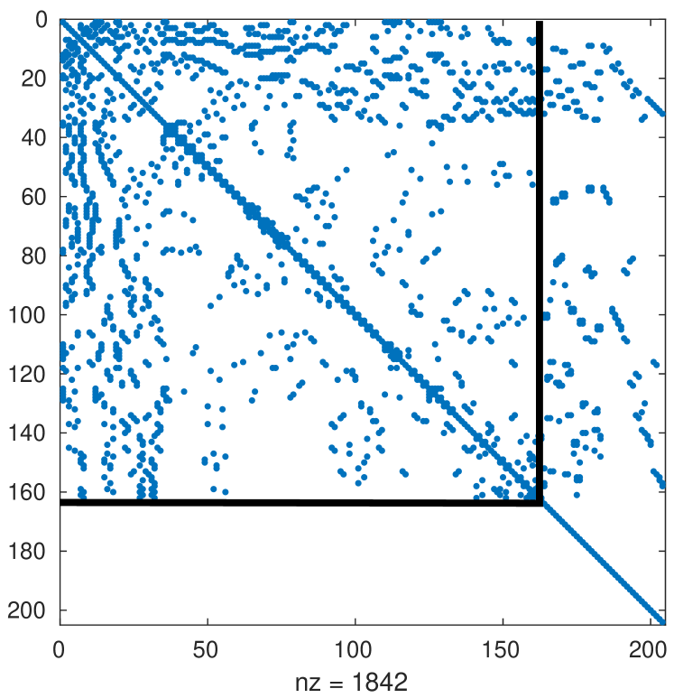
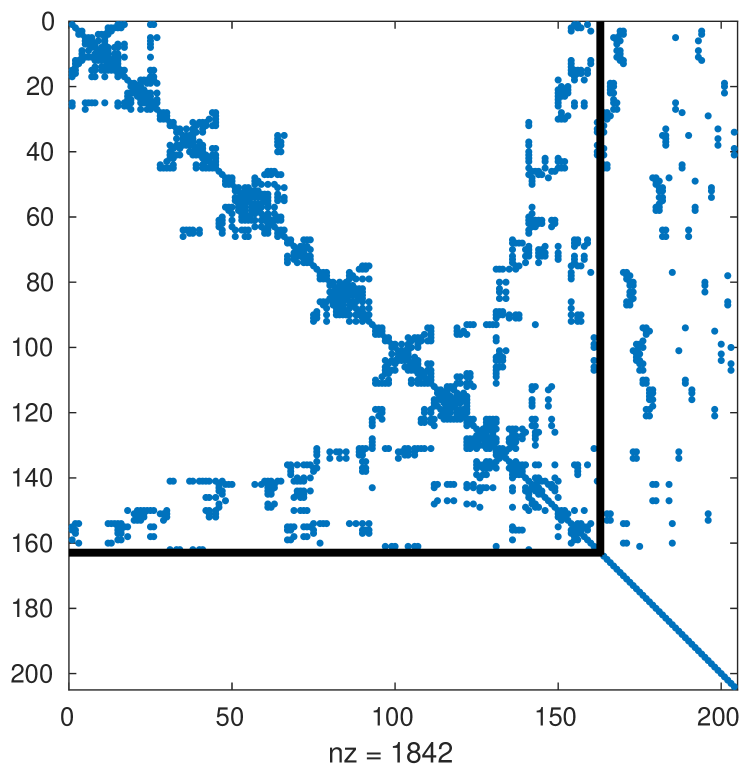
Figure 2: Sparsity pattern of a predominantly symmetric example matrix from FEM 2D before (left) and after MC64 matching and AMD reordering.

If $\boldsymbol{A}$ is fully nonsymmetric, i.e., $\boldsymbol{B}$ is empty, then we apply the nonsymmetric version of M64 and followed by symmetric AMD on $\boldsymbol{A}+\boldsymbol{A}^{T}$ to preserve the scaling effect. In this case, we have

$$\hat{\boldsymbol{A}}=\boldsymbol{P}_{r}^{T}\boldsymbol{D}_{r}\boldsymbol{A}\boldsymbol{D}_{c}\boldsymbol{P}_{c},$$ (9)

where $\boldsymbol{D}_{r}$ and $\boldsymbol{D}_{c}$ are row and column scaling matrices, and $\boldsymbol{P}_{r}^{T}$ and $\boldsymbol{P}_{c}$ are the row and column permutation matrices, respectively. Again, all the diagonals of $\hat{\boldsymbol{A}}$ have magnitude 1 due to matching and scaling.

We note two important special cases. First, symmetric matching and scaling may result in $2\times 2$ modulus-1 diagonal blocks, of which the diagonal entries may be small or even zero. To take advantage of these $2\times 2$ diagonal blocks, one must perform reordering on the block matrix followed by a block version of LDL${}^{\text{T}}$, which would significantly complicate the implementation and also introduce fills into the block rows and columns. For simplicity, we remove the part of $\boldsymbol{B}$ of which the diagonal entries are smaller than 1 after symmetric matching and defer them to the second level, where nonsymmetric matching will be used. Second, if matrix $\boldsymbol{A}$ has some nearly denser rows and columns, we will permute them to the lower right corners of $\boldsymbol{C}$ and tag them to prevent from diagonal pivoting. These operations may reduce the size of the block $\boldsymbol{A}_{1}$.

3.2 Incomplete LDL${}^{\text{T}}$ and LDU Factorization

After obtaining the preprocessed matrix $\hat{\boldsymbol{A}}$, we then compute the incomplete factorization. Since the leading symmetric block may be indefinite, we use incomplete LDL${}^{\text{T}}$ factorization instead of Cholesky factorization for the leading block, and we will use diagonal pivoting to control the growth of the inverse of the triangular factors, as described in Section 3.3. For a unified treatment of predominantly symmetric and nonsymmetric matrices, we use LDU factorization with diagonal pivoting, where $\boldsymbol{L}$ is unit lower triangular and $\boldsymbol{U}$ is unit upper triangular, and $\boldsymbol{U}=\boldsymbol{L}^{T}$ if $\hat{\boldsymbol{B}}$ is symmetric.

Let $\boldsymbol{P}$ denote the permutation matrix due to diagonal pivoting during the factorization process. The incomplete LDU factorization computes

$$\boldsymbol{P}^{T}\hat{\boldsymbol{A}}\boldsymbol{P}=\begin{bmatrix}\hat{\boldsymbol{B}}&\hat{\boldsymbol{F}}\\ \hat{\boldsymbol{E}}&\hat{\boldsymbol{C}}\end{bmatrix}\approx\begin{bmatrix}\tilde{\boldsymbol{B}}&\tilde{\boldsymbol{F}}\\ \tilde{\boldsymbol{E}}&\hat{\boldsymbol{C}}\end{bmatrix}=\begin{bmatrix}\boldsymbol{L}_{B}&0\\ \boldsymbol{L}_{E}&\boldsymbol{I}\end{bmatrix}\begin{bmatrix}\boldsymbol{D}_{B}&0\\ 0&\boldsymbol{S}_{C}\end{bmatrix}\begin{bmatrix}\boldsymbol{U}_{B}&\boldsymbol{U}_{F}\\ 0&\boldsymbol{I}\end{bmatrix},$$ (10)

where, $\hat{\boldsymbol{B}}\approx\tilde{\boldsymbol{B}}=\boldsymbol{L}_{B}\boldsymbol{D}_{B}\boldsymbol{U}_{B}$, $\hat{\boldsymbol{E}}\approx\tilde{\boldsymbol{E}}=\boldsymbol{L}_{E}\boldsymbol{D}_{B}\boldsymbol{U}_{B}$ and $\hat{\boldsymbol{F}}\approx\tilde{\boldsymbol{F}}=\boldsymbol{L}_{B}\boldsymbol{D}_{B}\boldsymbol{U}_{F}$. If $\hat{\boldsymbol{B}}$ is symmetric, then $\boldsymbol{U}_{B}=\boldsymbol{L}_{B}^{T}$ and $\tilde{\boldsymbol{B}}=\boldsymbol{L}_{B}\boldsymbol{D}_{B}\boldsymbol{L}_{B}^{T}$. Due to potential diagonal pivoting, $\hat{\boldsymbol{B}}$ may have fewer rows and columns than the leading block $\boldsymbol{A}_{1}$ in Section 3.1. The matrix $\boldsymbol{S}_{C}$ is the Schur complement, i.e., $\boldsymbol{S}_{C}=\hat{\boldsymbol{C}}-\boldsymbol{L}_{E}\boldsymbol{D}_{B}\boldsymbol{U}_{F}$.

We compute the incomplete LDU factorization using a procedure similar to the Crout version [28]. Let $\tilde{\boldsymbol{L}}$ and $\tilde{\boldsymbol{U}}$ denote $\begin{bmatrix}\boldsymbol{L}_{B}\\ \boldsymbol{L}_{E}\end{bmatrix}$ and $\begin{bmatrix}\boldsymbol{U}_{B}&\boldsymbol{U}_{F}\end{bmatrix}$, respectively. Let $\boldsymbol{\ell}_{k}$ and $\boldsymbol{u}_{k}^{T}$ denote the $k$th column of $\tilde{\boldsymbol{L}}$ and the $k$th row of $\tilde{\boldsymbol{U}}$, respectively, and let $\boldsymbol{D}_{k}$ denote the leading $k\times k$ block of $\boldsymbol{D}_{B}$. The Crout version builds $\tilde{\boldsymbol{L}}$ and $\tilde{\boldsymbol{U}}$ incrementally in columns and rows by computing

$$\boldsymbol{\ell}_{k} =\left(\boldsymbol{P}^{T}\hat{\boldsymbol{A}}\boldsymbol{P}\right)_{k+1:n,k}-\tilde{\boldsymbol{L}}_{k+1:n,1:k-1}\boldsymbol{D}_{k-1}\tilde{\boldsymbol{U}}_{1:k-1,k}$$ (11)

$$\boldsymbol{u}_{k}^{T} =\left(\boldsymbol{P}^{T}\hat{\boldsymbol{A}}\boldsymbol{P}\right)_{k,k+1:n}-\tilde{\boldsymbol{L}}_{k,1:k-1}\boldsymbol{D}_{k-1}\tilde{\boldsymbol{U}}_{1:k-1:k+1:n}$$ (12)

at the $k$th step. The left panel of Figure 3 illustrates the update of $\boldsymbol{\ell}_{k}$; and the update of $\boldsymbol{u}_{k}^{T}$ is done symmetrically. The right panel of Figure 3 illustrates the details of updating and dropping, which we will explain in Section 4.2.1. In PS-MILU, the entries of $\boldsymbol{u}_{k}^{T}$ within $\boldsymbol{U}_{B}$ are equal to their corresponding entries in $\boldsymbol{\ell}_{k}$, so we can save their computational cost by half. However, those in $\boldsymbol{U}_{F}$ must be updated separately from $\boldsymbol{L}_{E}$. If $\hat{\boldsymbol{A}}$ is fully nonsymmetric, the same procedure described above applies by updating the whole $\boldsymbol{u}_{k}^{T}$.

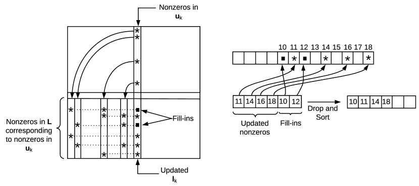
Figure 3: Illustration of updating $\boldsymbol{\ell}_{k}$ in Crout update.

Compared to the classical LU factorization procedures, which update the Schur complement at the $k$th step, the Crout version allows easier incorporation of dropping in $\boldsymbol{\ell}_{k}$ and $\boldsymbol{u}_{k}^{T}$, as we will describe shortly. The Crout procedure in [28] did not support diagonal pivoting. For effective pivoting, we update $\boldsymbol{D}_{B}$ after computing $\boldsymbol{\ell}_{k}$ and $\boldsymbol{u}_{k}^{T}$ at step $k$, before applying droppings to $\boldsymbol{\ell}_{k}$ and $\boldsymbol{u}_{k}^{T}$. Specifically, let $\boldsymbol{d}^{(k-1)}$ denote the vector containing the partial result of $\boldsymbol{D}_{B}$ from the step $k-1$, where $\boldsymbol{d}^{(0)}$ is initialized to the diagonal entries of $\hat{\boldsymbol{B}}$. Let $\boldsymbol{\ell}_{B,k}$ and $\boldsymbol{u}_{B,k}^{T}$ denote the $\boldsymbol{L}_{B}$ and $\boldsymbol{U}_{B}$ portions of $\boldsymbol{\ell}_{k}$ and $\boldsymbol{u}_{k}^{T}$, respectively. Then,

$$\boldsymbol{d}_{k+1:m}^{(k)}=\boldsymbol{d}_{k+1:m}^{(k-1)}-d_{k}\boldsymbol{\ell}_{B,k}.*\boldsymbol{u}_{B,k}^{T},$$ (13)

where $m$ is the size of $\hat{\boldsymbol{B}}$ and $.*$ denotes element-wise multiplication. When diagonal pivoting is performed, we will need to permute entries in $\boldsymbol{d}$, along with the rows in $\tilde{\boldsymbol{L}}$ and columns in $\tilde{\boldsymbol{U}}$, which we describe next.

3.3 Diagonal Pivoting

One of the crucial components in PS-MILU is diagonal pivoting. For nonsymmetric systems, diagonal pivoting has been shown to be very effective [7]. For symmetric systems, the importance of pivoting is at least as important as for nonsymmetric cases, for at least two reasons. First, as a direct method, LDL${}^{\text{T}}$ without pivoting may break down for indefinite systems. A simplest example is $\boldsymbol{A}=\begin{bmatrix}0&1\\ 1&0\end{bmatrix}.$ A direct implication of this fact is that incomplete LDL${}^{\text{T}}$ without pivoting can suffer from instability for symmetric and indefinite systems. A well-known factorization for symmetric and indefinite systems is block LDL${}^{\text{T}}$ with diagonal pivoting [12], which requires $1\times 1$ and $2\times 2$ diagonal blocks. Even though it may be possible that block LDL with much larger blocks can be stable without pivoting across blocks, but pivoting may still be needed within blocks.

The second reason is that for incomplete factorizations, diagonal pivoting is important in controlling the growth of the inverse of the triangular factors. This can be shown as follows. Consider the incomplete LDU factorization with pivoting,

$$\boldsymbol{P}^{T}\hat{\boldsymbol{A}}\boldsymbol{Q}=\boldsymbol{L}\boldsymbol{D}\boldsymbol{U}+\boldsymbol{\delta}_{A},$$ (14)

where $\boldsymbol{\delta}_{A}$ is the error due to dropping. Let $\boldsymbol{M}=\boldsymbol{L}\boldsymbol{D}\boldsymbol{U}$ be a right-preconditioner of $\boldsymbol{P}^{T}\hat{\boldsymbol{A}}\boldsymbol{Q}$. Then,

$$\boldsymbol{P}^{T}\hat{\boldsymbol{A}}\boldsymbol{Q}\boldsymbol{M}^{-1}=\boldsymbol{I}+\boldsymbol{\delta}_{A}\boldsymbol{M}^{-1}=\boldsymbol{I}+\boldsymbol{\delta}_{A}\boldsymbol{U}^{-1}\boldsymbol{D}^{-1}\boldsymbol{L}^{-1},$$ (15)

where the spectral radius of the second term is bounded by

$$\rho\left(\boldsymbol{\delta}_{A}\boldsymbol{M}^{-1}\right) \leq\left\|\boldsymbol{\delta}_{A}\boldsymbol{U}^{-1}\boldsymbol{D}^{-1}\boldsymbol{L}^{-1}\right\|$$ (16)

$$\,\leq\left\|\boldsymbol{D}^{-1}\right\|\left\|\boldsymbol{L}^{-1}\right\|\left\|\boldsymbol{U}^{-1}\right\|\left\|\boldsymbol{\delta}_{A}\right\|.$$ (17)

Therefore, $\left\|\boldsymbol{D}^{-1}\right\|\left\|\boldsymbol{L}^{-1}\right\|\left\|\boldsymbol{U}^{-1}\right\|$ is an absolute condition number for the spectral radius of the preconditioned matrix $\boldsymbol{P}^{T}\hat{\boldsymbol{A}}\boldsymbol{Q}\boldsymbol{M}^{-1}$ with respect to $\left\|\boldsymbol{\delta}_{A}\right\|$. For a well-scaled matrix $\hat{\boldsymbol{A}}$, $\left\|\boldsymbol{\delta}_{A}\right\|$ is well bounded, and $\left\|\boldsymbol{D}^{-1}\right\|$ is typically small. However, a large $\left\|\boldsymbol{L}^{-1}\right\|$ or $\left\|\boldsymbol{U}^{-1}\right\|$ can significantly deteriorate the spectral radius, which in turn can undermine the convergence of the preconditioned KSP method. Note that even with block LDL${}^{\text{T}}$ without pivoting, $\left\|\boldsymbol{L}^{-1}\right\|$ and $\left\|\boldsymbol{U}^{-1}\right\|$ may still grow rapidly. Therefore, we consider pivoting indispensable for the robustness of incomplete factorization.

Estimating the 2-norms are relatively expensive. However, we can estimate and bound the $\infty$-norm of the inverse of a triangular matrix efficiently, in that

$$\left\|\boldsymbol{T}^{-1}\right\|_{\infty}=\sup_{\|\boldsymbol{v}\|_{\infty}=1}\left\|\boldsymbol{T}^{-1}\boldsymbol{v}\right\|_{\infty}\gtrapprox\sup_{c_{i}=\pm 1}\left\|\boldsymbol{T}^{-1}\boldsymbol{c}\right\|_{\infty},$$ (18)

where the sign of $c_{i}$ is chosen in a greedy fashion to maximize $\left|\boldsymbol{e}_{i}^{T}\boldsymbol{T}^{-1}\boldsymbol{c}\right|$; see [16, 25] for more detail. In the context of LDU factorization, let $\boldsymbol{L}_{k}$ and $\boldsymbol{U}_{k}$ denote the leading $k\times k$ blocks of $\boldsymbol{L}$ and $\boldsymbol{U}$, respectively, and let $\boldsymbol{c}_{L,k}$ and $\boldsymbol{c}_{U,k}$ denote their corresponding $\boldsymbol{c}$ vectors in (18). We can bound $\left\|\boldsymbol{L}_{k}^{-1}\right\|_{\infty}$ incrementally: Given that $\left\|\boldsymbol{L}_{k-1}^{-1}\boldsymbol{c}_{L,k-1}\right\|_{\infty}\leq\tau_{\kappa}$ for some threshold $\tau_{\kappa}$ as estimated greedily based on (18), then $\left\|\boldsymbol{L}_{k}^{-1}\boldsymbol{c}_{L,k}\right\|_{\infty}>\tau_{\kappa}$ based on the same estimation if and only if

$$\tilde{\kappa}_{L,k}=\left|\boldsymbol{e}_{k}^{T}\boldsymbol{L}_{k}^{-1}\boldsymbol{c}_{L,k}\right|>\tau_{k},$$ (19)

where $\boldsymbol{e}_{k}\in\mathbb{R}^{k}$. Similarly, we can bound $\left\|\boldsymbol{U}_{k}^{-1}\right\|_{1}=\left\|\boldsymbol{U}_{k}^{-T}\right\|_{\infty}$ by estimating

$$\tilde{\kappa}_{U,k}=\left|\boldsymbol{e}_{k}^{T}\boldsymbol{U}_{k}^{-T}\boldsymbol{c}_{U,k}\right|,$$ (20)

where $\tilde{\kappa}_{U,k}=\tilde{\kappa}_{L,k}$ for symmetric $\hat{\boldsymbol{B}}$.

It is easy to incorporate the estimation of the condition numbers into the Crout update. In particular, after computing $\boldsymbol{\ell}_{k}$ and $\boldsymbol{u}_{k}^{T}$ at the $k$th step, we incrementally update $\boldsymbol{c}_{L,k}$, $\boldsymbol{c}_{U,k}$, $\boldsymbol{L}_{k}^{-1}\boldsymbol{c}_{L,k}$ and $\boldsymbol{U}_{k}^{-T}\boldsymbol{c}_{U,k}$ from their partial results in step $k-1$, compute $\tilde{\kappa}_{L,k}$ and $\tilde{\kappa}_{U,k}$, and then compare them with the threshold $\tau_{\kappa}$. According to (17), we also need to safeguard $\left\|\boldsymbol{D}^{-1}\right\|$ by comparing $\left|1/d_{k}\right|$ against a threshold $\tau_{d}$. Let $m$ denote the size of $\hat{\boldsymbol{B}}$. If $\max\{\tilde{\kappa}_{L,k},\tilde{\kappa}_{U,k}\}>\tau_{\kappa}$, or $|1/d_{k}|>\tau_{d}$, we exchange row $k$ and column $k$ in $\hat{\boldsymbol{A}}$ with the $m$th row and column of $\hat{\boldsymbol{A}}$, reduce the size of $\hat{\boldsymbol{B}}$ (i.e., $m$) by one, and recompute the Crout update. Figure 4 illustrates this pivot operation. This process repeats until $\tilde{\kappa}_{L,k}$, $\tilde{\kappa}_{U,k}$, and $|1/d_{k}|$ are all within threshold or the leading block has been exhausted. Since we have pre-updated $\boldsymbol{D}$ in the modified Crout update, we check $|1/d_{m}|$ before pivoting and reduce $m$ by $1$ if $|1/d_{m}|<\tau_{d}$ directly. This avoids unnecessary exchanges if $\left|d_{m}\right|$ is small. In terms of implementation, special care must be taken to ensure optimal time complexity, which we will address in Section 4.

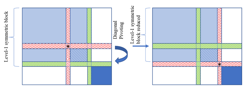
Figure 4: Illustration of diagonal pivoting for level-$1$ symmetric block. It removes “problematic” rows and columns from the current level and merge them with the block for more robust processing in the next level.

3.4 Inverse-Based Thresholding

For incomplete factorization to be effective, it must balance two important factors: first, it must control the numbers of nonzeros in $\boldsymbol{L}$ and $\boldsymbol{U}$, which ideally should be linear in the input size. This requires dropping “insignificant” nonzeros in $\boldsymbol{L}$ and $\boldsymbol{U}$. Second, as shown above, it is important to control $\left\|\boldsymbol{D}^{-1}\right\|\left\|\boldsymbol{L}^{-1}\right\|\left\|\boldsymbol{U}^{-1}\right\|$, which determine the spectral radius of the preconditioned matrix. For this reason, the traditional dropping criteria, such as those based on the level in the elimination tree or the magnitude of the entries, are often ineffective. A robust approach is the inverse-based thresholding proposed in [7]. We adopt this approach, but we pay special attention to achieve optimal time complexity in terms of the number of fills and the computational cost.

The inverse-based thresholding can be motivated by an argument similar to, but more detailed than, the analysis in the preceding subsection. In particular, let

$$\boldsymbol{P}^{T}\hat{\boldsymbol{A}}\boldsymbol{Q} =\left(\boldsymbol{L}+\boldsymbol{\delta}_{L}\right)\left(\boldsymbol{D}+\boldsymbol{\delta}_{D}\right)\left(\boldsymbol{U}+\boldsymbol{\delta}_{U}\right)$$

$$=\boldsymbol{L}\boldsymbol{D}\boldsymbol{U}+\boldsymbol{\delta}_{L}\boldsymbol{D}\boldsymbol{U}+\boldsymbol{L}\boldsymbol{D}\boldsymbol{\delta}_{U}+\boldsymbol{L}\boldsymbol{\delta}_{D}\boldsymbol{U}+\text{h.o.t.},$$ (21)

where we omit the higher-order terms that involve more than one $\boldsymbol{\delta}$ matrix. Let $\boldsymbol{M}=\boldsymbol{L}\boldsymbol{D}\boldsymbol{U}$ be a right preconditioner of $\boldsymbol{P}^{T}\hat{\boldsymbol{A}}\boldsymbol{Q}$. Similar to (16),

$$\rho\left(\boldsymbol{\delta}_{A}\boldsymbol{M}^{-1}\right) \approx\rho\left(\left(\boldsymbol{\delta}_{L}\boldsymbol{D}\boldsymbol{U}+\boldsymbol{L}\boldsymbol{D}\boldsymbol{\delta}_{U}+\boldsymbol{L}\boldsymbol{\delta}_{D}\boldsymbol{U}\right)\boldsymbol{M}^{-1}\right)$$

$$\leq\left\|\boldsymbol{\delta}_{L}\boldsymbol{L}^{-1}+\boldsymbol{L}\boldsymbol{D}\boldsymbol{\delta}_{U}\boldsymbol{U}^{-1}\boldsymbol{D}^{-1}\boldsymbol{L}^{-1}+\boldsymbol{L}\boldsymbol{\delta}_{D}\boldsymbol{D}^{-1}\boldsymbol{L}^{-1}\right\|$$

$$\leq\left\|\boldsymbol{\delta}_{L}\boldsymbol{L}^{-1}\right\|+\kappa(\boldsymbol{M})\left\|\boldsymbol{U}^{-1}\boldsymbol{\delta}_{U}\right\|+\kappa(\boldsymbol{L})\left\|\boldsymbol{\delta}_{D}\boldsymbol{D}^{-1}\right\|.$$ (22)

When deciding whether to drop a specific $\ell_{ik}$, consider $\boldsymbol{\delta}{}_{ik}=\ell_{ik}\hat{\boldsymbol{e}}_{i}\hat{\boldsymbol{e}}_{k}^{T}$, where $i\geq k$ and $\hat{\boldsymbol{e}}_{i},\hat{\boldsymbol{e}}_{k}\in\mathbb{R}^{n}$. Then,

$$\left\|\boldsymbol{\delta}{}_{ik}\boldsymbol{L}^{-1}\right\|=\left\|\ell_{ik}\hat{\boldsymbol{e}}_{i}\hat{\boldsymbol{e}}_{k}^{T}\boldsymbol{L}^{-1}\right\|=\left|\ell_{ik}\right|\left\|\hat{\boldsymbol{e}}_{k}^{T}\boldsymbol{L}^{-1}\right\|=\left|\ell_{ik}\right|\left\|\boldsymbol{e}_{k}^{T}\boldsymbol{L}_{k}^{-1}\right\|,$$ (23)

where $\boldsymbol{e}_{k}\in\mathbb{R}^{k}$. Instead of estimating the 2-norm, we can estimate the $\infty$-norm as

$$\left\|\boldsymbol{e}_{k}^{T}\boldsymbol{L}_{k}^{-1}\right\|_{\infty}=\sup_{c_{i}=\pm 1}\left|\boldsymbol{e}_{k}^{T}\boldsymbol{L}_{k}^{-1}\boldsymbol{c}\right|\gtrapprox\left|\boldsymbol{e}_{k}^{T}\boldsymbol{L}_{k}^{-1}\boldsymbol{c}_{L,k}\right|=\tilde{\kappa}_{L,k},$$ (24)

where $\boldsymbol{c}_{L,k}$ and $\tilde{\kappa}_{L,k}$ were defined in Section 3.3. Similarly, let $\boldsymbol{\delta}{}_{kj}=u_{kj}\hat{\boldsymbol{e}}_{k}\hat{\boldsymbol{e}}_{j}^{T}$, we then have

$$\left\|\boldsymbol{U}^{-1}\boldsymbol{\delta}{}_{kj}\right\|=\left\|\boldsymbol{U}^{-1}\left(u_{ki}\hat{\boldsymbol{e}}_{k}\hat{\boldsymbol{e}}_{j}^{T}\right)\right\|=\left|u_{kj}\right|\left\|\boldsymbol{e}_{k}^{T}\boldsymbol{U}_{k}^{-T}\right\|,$$ (25)

and $\left\|\boldsymbol{e}_{k}^{T}\boldsymbol{U}_{k}^{-T}\right\|_{\infty}\gtrapprox\left|\boldsymbol{e}_{k}^{T}\boldsymbol{U}_{k}^{-T}\boldsymbol{c}_{U,k}\right|=\tilde{\kappa}_{U,k}$. Therefore, as a heuristic, we drop $\ell_{ik}$ if

$$\left|\ell_{ik}\right|\tilde{\kappa}_{L,k}\leq\tau_{L}$$ (26)

and drop $u_{kj}$ if

$$\left|u_{kj}\right|\tilde{\kappa}_{U,k}\leq\tau_{U}$$ (27)

for some $\tau_{L}$ and $\tau_{U}$. This is referred to as the inverse-based thresholding [28, 7]. To control the time complexity of the algorithm, we also limit the numbers of nonzeros in $\boldsymbol{\ell}_{k}$ and $\boldsymbol{u}_{k}^{T}$ to be within constant factors (specifically, $\alpha_{L}$ and $\alpha_{U}$) of the numbers of nonzeros in the corresponding row and column in $\boldsymbol{P}^{T}\hat{\boldsymbol{A}}\boldsymbol{Q}$, and drop the excess nonzeros even if their values are above the threshold $\tau_{L}/\tilde{\kappa}_{L,k}$ and $\tau_{U}/\tilde{\kappa}_{U,k}$.

This dropping technique can be easily incorporated into the modified Crout update procedure, in that $\tilde{\kappa}_{L,k}$ and $\tilde{\kappa}_{U,k}$ have already been computed. According to (22), assuming $\boldsymbol{M}$ is used as a right-preconditioner, the spectral radius is the most sensitive to $\boldsymbol{\delta}_{U}$, followed by $\boldsymbol{\delta}_{D}$ and $\boldsymbol{\delta}_{L}$ in that order. To reduce $\boldsymbol{\delta}_{D}$, we update $\boldsymbol{D}$ before applying dropping to $\boldsymbol{\ell}_{k}$ and $\boldsymbol{u}_{k}^{T}$ in the modified Crout update, as we mentioned Section 3.3. Furthermore, to compensate the sensitivity of $\boldsymbol{\delta}_{U}$, it is advantageous for $\tau_{U}\leq\tau_{L}$ and $\alpha_{U}\geq\alpha_{L}$. For a symmetric leading block, we let $\tau_{L}=\tau_{U}$ and $\alpha_{L}=\alpha_{U}$.

3.5 Hybrid Schur Complement

Another key component is the computation of the Schur complement, which will be factorized in the next level. From (10), the Schur complement is defined as

$$\boldsymbol{S}_{C} =\left[\begin{array}[]{cc}-\boldsymbol{L}_{E}\boldsymbol{L}_{B}^{-1}&\boldsymbol{I}\end{array}\right]\begin{bmatrix}\tilde{\boldsymbol{B}}&\tilde{\boldsymbol{F}}\\ \tilde{\boldsymbol{E}}&\hat{\boldsymbol{C}}\end{bmatrix}\left[\begin{array}[]{c}-\boldsymbol{U}_{B}^{-1}\boldsymbol{U}_{F}\\ \boldsymbol{I}\end{array}\right]$$ (31)

$$=\hat{\boldsymbol{C}}-\boldsymbol{L}_{E}\boldsymbol{D}_{B}\boldsymbol{U}_{F}.$$ (32)

Note that $\hat{\boldsymbol{C}}$ was permuted and scaled, but it involves no dropping. However, $\tilde{\boldsymbol{B}}$, $\tilde{\boldsymbol{E}}$, and $\tilde{\boldsymbol{F}}$ do involve dropping, and the above definition does not take into account the effect of dropping on the preconditioned matrix. Let $\boldsymbol{M}^{-1}=\begin{bmatrix}\tilde{\boldsymbol{B}}&\tilde{\boldsymbol{F}}\\ \tilde{\boldsymbol{E}}&\hat{\boldsymbol{C}}\end{bmatrix}$, and $\boldsymbol{P}^{T}\hat{\boldsymbol{A}}\boldsymbol{P}\boldsymbol{M}^{-1}=\begin{bmatrix}\hat{\boldsymbol{B}}&\hat{\boldsymbol{F}}\\ \hat{\boldsymbol{E}}&\hat{\boldsymbol{C}}\end{bmatrix}\begin{bmatrix}\tilde{\boldsymbol{B}}&\tilde{\boldsymbol{F}}\\ \tilde{\boldsymbol{E}}&\hat{\boldsymbol{C}}\end{bmatrix}^{-1}$. The errors in $\boldsymbol{\delta}_{B}=\hat{\boldsymbol{B}}-\tilde{\boldsymbol{B}}$ can be magnified by both $\boldsymbol{L}_{B}^{-1}$ and $\boldsymbol{U}_{B}^{-1}$, as we shall show shortly. Hence, we introduce a modified formula for the Schur complement,

$$\boldsymbol{H}_{C} =\boldsymbol{C}-2\boldsymbol{L}_{E}\boldsymbol{D}_{B}\boldsymbol{U}_{F}+\boldsymbol{L}_{E}\boldsymbol{L}_{B}^{-1}\hat{\boldsymbol{B}}\boldsymbol{U}_{B}^{-1}\boldsymbol{U}_{F}$$ (33)

$$=\boldsymbol{S}_{C}+\boldsymbol{L}_{E}\left(\boldsymbol{L}_{B}^{-1}\hat{\boldsymbol{B}}\boldsymbol{U}_{B}^{-1}-\boldsymbol{D}_{B}\right)\boldsymbol{U}_{F},$$ (34)

where the second term eliminates this error term due to $\boldsymbol{\delta}_{B}$.

To derive (33), let us first define a preconditioner $\hat{\boldsymbol{M}}$ as

$$\hat{\boldsymbol{M}}=\begin{bmatrix}\boldsymbol{I}&0\\ \boldsymbol{L}_{E}\boldsymbol{L}_{B}^{-1}&\boldsymbol{I}\end{bmatrix}\begin{bmatrix}\tilde{\boldsymbol{B}}&0\\ 0&\boldsymbol{T}_{C}\end{bmatrix}\begin{bmatrix}\boldsymbol{I}&\boldsymbol{U}_{B}^{-1}\boldsymbol{U}_{F}\\ 0&\boldsymbol{I}\end{bmatrix},$$ (35)

where $\boldsymbol{T}_{C}$ has yet to be defined. Then,

$$\rho\left(\boldsymbol{P}^{T}\hat{\boldsymbol{A}}\boldsymbol{P}\hat{\boldsymbol{M}}^{-1}\right) =\rho\left(\begin{bmatrix}\boldsymbol{I}&0\\ \boldsymbol{L}_{E}\boldsymbol{L}_{B}^{-1}&\boldsymbol{I}\end{bmatrix}^{-1}\begin{bmatrix}\hat{\boldsymbol{B}}&\hat{\boldsymbol{F}}\\ \hat{\boldsymbol{E}}&\hat{\boldsymbol{C}}\end{bmatrix}\begin{bmatrix}\boldsymbol{I}&\boldsymbol{U}_{B}^{-1}\boldsymbol{U}_{F}\\ 0&\boldsymbol{I}\end{bmatrix}^{-1}\begin{bmatrix}\tilde{\boldsymbol{B}}&0\\ 0&\boldsymbol{T}_{C}\end{bmatrix}^{-1}\right)$$

$$=\rho\left(\begin{bmatrix}\boldsymbol{I}&0\\ -\boldsymbol{L}_{E}\boldsymbol{L}_{B}^{-1}&\boldsymbol{I}\end{bmatrix}\begin{bmatrix}\hat{\boldsymbol{B}}&\hat{\boldsymbol{F}}\\ \hat{\boldsymbol{E}}&\hat{\boldsymbol{C}}\end{bmatrix}\begin{bmatrix}\boldsymbol{I}&-\boldsymbol{U}_{B}^{-1}\boldsymbol{U}_{F}\\ 0&\boldsymbol{I}\end{bmatrix}\begin{bmatrix}\tilde{\boldsymbol{B}}&0\\ 0&\boldsymbol{T}_{C}\end{bmatrix}^{-1}\right)$$

$$=\rho\left(\begin{bmatrix}\hat{\boldsymbol{B}}&\hat{\boldsymbol{\delta}}_{F}\\ \hat{\boldsymbol{\delta}}_{E}&\hat{\boldsymbol{T}}_{C}\end{bmatrix}\begin{bmatrix}\tilde{\boldsymbol{B}}&0\\ 0&\boldsymbol{T}_{C}\end{bmatrix}^{-1}\right).$$

where $\hat{\boldsymbol{\delta}}_{E}$ and $\hat{\boldsymbol{\delta}}_{F}$ correspond to the effect of dropping in $\hat{\boldsymbol{E}}$ and $\hat{\boldsymbol{F}}$, respectively. Suppose $\hat{\boldsymbol{\delta}}_{E}$ and $\hat{\boldsymbol{\delta}}_{F}$ are small, and the above spectral radius is approximately minimized if $\hat{\boldsymbol{T}}_{C}\boldsymbol{T}_{C}^{-1}=\boldsymbol{I}$, i.e.,

$$\boldsymbol{T}_{C}=\hat{\boldsymbol{T}}_{C} =\left[\begin{array}[]{cc}-\boldsymbol{L}_{E}\boldsymbol{L}_{B}^{-1}&\boldsymbol{I}\end{array}\right]\begin{bmatrix}\hat{\boldsymbol{B}}&\hat{\boldsymbol{F}}\\ \hat{\boldsymbol{E}}&\hat{\boldsymbol{C}}\end{bmatrix}\left[\begin{array}[]{c}-\boldsymbol{U}_{B}^{-1}\boldsymbol{U}_{F}\\ \boldsymbol{I}\end{array}\right]$$ (39)

$$=\boldsymbol{L}_{E}\boldsymbol{L}_{B}^{-1}\hat{\boldsymbol{B}}\boldsymbol{U}_{B}^{-1}\boldsymbol{U}_{F}-\hat{\boldsymbol{E}}\boldsymbol{U}_{B}^{-1}\boldsymbol{U}_{F}-\boldsymbol{L}_{E}\boldsymbol{L}_{B}^{-1}\hat{\boldsymbol{F}}+\hat{\boldsymbol{C}}.$$ (40)

This formulation of Schur complement was introduced in [40] and was also used in [10]. Bollhöfer and Saad [10] referred to (31) and (39) as the S-version and T-version, respectively. However, $\boldsymbol{T}_{C}$ is relatively complicated. Note that

$$\boldsymbol{T}_{C}-\boldsymbol{S}_{C} =\left[\begin{array}[]{cc}-\boldsymbol{L}_{E}\boldsymbol{L}_{B}^{-1}&\boldsymbol{I}\end{array}\right]\begin{bmatrix}\boldsymbol{\delta}_{B}&\boldsymbol{\delta}_{F}\\ \boldsymbol{\delta}_{E}&\boldsymbol{0}\end{bmatrix}\left[\begin{array}[]{c}-\boldsymbol{U}_{B}^{-1}\boldsymbol{U}_{F}\\ \boldsymbol{I}\end{array}\right]$$ (44)

$$=\boldsymbol{L}_{E}\boldsymbol{L}_{B}^{-1}\boldsymbol{\delta}_{B}\boldsymbol{U}_{B}^{-1}\boldsymbol{U}_{F}-\boldsymbol{\delta}_{E}\boldsymbol{U}_{B}^{-1}\boldsymbol{U}_{F}-\boldsymbol{L}_{E}\boldsymbol{L}_{B}^{-1}\boldsymbol{\delta}_{F}.$$ (45)

Note that $\boldsymbol{\delta}_{E}$ and $\boldsymbol{\delta}_{F}$ are multiplied by $\boldsymbol{U}_{B}^{-1}$ and $\boldsymbol{L}_{B}^{-1}$, respectively, so their effects are similar to the droppings in $\boldsymbol{L}_{B}$ in (22). However, $\boldsymbol{\delta}_{B}$ is multiplied by both $\boldsymbol{L}_{B}^{-1}$ and $\boldsymbol{U}_{B}^{-1}$, which can “square the condition number.” Eq. (33) adds the leading term in (45) to $\boldsymbol{S}_{C}$ to obtain $\boldsymbol{H}_{C}$ and in turn avoids the “squaring” effect. Note that

$$\boldsymbol{H}_{C}=\left[\begin{array}[]{cc}-\boldsymbol{L}_{E}\boldsymbol{L}_{B}^{-1}&\boldsymbol{I}\end{array}\right]\begin{bmatrix}\hat{\boldsymbol{B}}&\tilde{\boldsymbol{F}}\\ \tilde{\boldsymbol{E}}&\hat{\boldsymbol{C}}\end{bmatrix}\left[\begin{array}[]{c}-\boldsymbol{U}_{B}^{-1}\boldsymbol{U}_{F}\\ \boldsymbol{I}\end{array}\right],$$ (46)

which can be viewed as a hybrid of $\boldsymbol{S}_{C}$ and $\boldsymbol{T}_{C}$ in (31) and (39), respectively. Therefore, we refer to $\boldsymbol{H}_{C}$ as the hybrid version, or H-version, of the Schur complement. The H-version has similar accuracy as the T-version, and it is simpler and can be computed as an update to $\boldsymbol{S}_{C}$.

In both the H- and the T-version, the term $\boldsymbol{L}_{E}\boldsymbol{L}_{B}^{-1}\hat{\boldsymbol{B}}\boldsymbol{U}_{B}^{-1}\boldsymbol{U}_{F}$ can potentially make the Schur complement dense. Hence, we use the S-version without dropping for almost all levels. Let $n_{C}$ denote the size of $\hat{\boldsymbol{C}}$ at a particular level. If the Schur complement is small (in particular, $n_{C}=\mathcal{O}(n^{1/3})$) or the S-version is nearly dense, then we would apply a dense complete LU factorization with column pivoting to factorize it; otherwise, we factorize $\boldsymbol{S}_{C}$ using multilevel ILU recursively. We update the Schur complement to the H-version if $n_{C}$ is smaller than a user-specified $c_{h}$. We will address the complexity analysis in more detail in Section 4.3. After obtaining the multilevel ILU, one can then use (6) recursively to construct a preconditioner.

4 Implementation Details and Complexity Analysis

The preceding section focused on the robustness of PS-MILU. In this section, we address its efficient implementation, to achieve optimal time complexity. More specifically, if the number of nonzeros per row and per column are bounded by a constant, the algorithm and its implementation must scale linearly with respect to the input size. To the best our knowledge, the only methods in the literature that could achieve linear-time complexity are ILU0 or ILUT without pivoting, which unfortunately are not robust. As demonstrated in [24], multilevel ILU scales nearly linearly for certain classes of problems, but there was no theoretical complexity analysis in the literature.

To achieve optimal complexity for PS-MILU, we must have a data structure for sparse matrices that supports efficient sequential access of a matrix in amortized constant time per nonzero in both row and column major, while supporting efficient row or column interchanges. In addition, the costs of thresholding, pivoting, and sorting must not dominate the intrinsic floating-point operations in the incomplete LU factorization. In the following, we will describe our data structures, present the pseudocode, and then prove the optimal time complexity of our algorithm.

4.1 An Augmented Sparse Matrix Storage

To facilitate the implementation of PS-MILU, we need an efficient data structure for sparse matrices, whose storage requirement must be linear in the number of nonzeros. In the Crout update, we need to access both rows and columns of $\boldsymbol{P}^{T}\hat{\boldsymbol{A}}\boldsymbol{Q}$, $\boldsymbol{L}$, and $\boldsymbol{U}$, and it is critical that the access time is constant per nonzero in an amortized sense. The standard storage formats, such as AIJ, CCS (Compressed Column Storage), or CRS (Compressed Row Storage), are insufficient for this purpose. In addition, we must facilitate row interchanges in $\boldsymbol{L}$ and column interchanges in $\boldsymbol{U}$ efficiently, while taking into account the cache performance of the Crout update as much as possible.

To this end, we introduce a data structure that augments the CCS or CRS formats, which we refer to as Augmented Compressed Column Storage (AugCCS) and Augmented Compressed Row Storage (AugCRS), respectively. Like CCS and CRS, our data structure is array based so that it can be easily implemented in any programming language, such as MATLAB, FORTRAN, C/C++, etc. The two versions are interchangeable in functionality, but they may deliver different cache performance depending on the locality of the algorithm. We will use AugCCS and AugCRS for $\boldsymbol{L}$ and $\boldsymbol{U}$, respectively, because PS-MILU primarily accesses $\boldsymbol{L}$ in columns and primarily accesses $\boldsymbol{U}$ in rows. In the following, we shall describe AugCCS for $\boldsymbol{L}$.

Our primary design goals of AugCCS include building $\boldsymbol{L}$ incrementally in columns in the Crout update, efficient sequential access in both rows and columns, efficient search of row indices, and efficient implementation of row interchanges. Recall that the standard CCS format has the following collection of arrays:

• row_ind: An integer array of size equal to the total number of nonzeros, storing the row indices of the nonzeros in each column;

• col_start: An integer array of size $n+1$, storing the start index of each column in row_ind, where col_start[k+1]-1 is the end index for the $k$th column;

• val: A floating-point array of the same size as row_ind, storing the nonzero values in each column.

In CCS, row_ind and val have the same memory layout and are accessed based on the same indexing. Because the number of nonzeros in $\boldsymbol{\ell}_{k}$ is not known until the end of step $k$ of Crout update, we cannot determine col_start a priori, so col_start[k+1] must be updated incrementally at the end of the $k$th step. However, for efficiency, we can estimate the total number of nonzeros in $\boldsymbol{L}$ and reserve storage for row_ind and val a priori, because we control the number of the nonzeros in $\boldsymbol{\ell}_{k}$ to be within a constant factor of that in its corresponding column in $\boldsymbol{P}^{T}\hat{\boldsymbol{A}}\boldsymbol{P}$.

In CCS, the sorting of the indices in row_ind is optional. In AugCCS, we require the indices to be sorted in ascending order. The sorting may be counterintuitive, because it would incur additional cost when appending a column $\boldsymbol{\ell}_{k}$ and when performing row interchanges. Sorting entries in $\boldsymbol{\ell}_{k}$ has a lower time complexity compared to computing $\boldsymbol{\ell}_{k}$. In terms of row interchanges, if rows $k$ and $i$ in $\boldsymbol{L}$ are interchanged at step $k$ of the Crout update, where $i>k$, we need to update the sorted indices in the $j$th column in row_ind and in val if $\ell_{kj}$ or $\ell_{ij}$ is nonzero. The total amount of data movement is linear in the number of nonzeros within these columns, which is asymptotically optimal for pivoting using a sparse storage format, as we will show in Section 4.3. With sorted lists, we can optimize other steps of the algorithm.

A main limitation of CCS is that it does not allow constant-time access of nonzeros of $\boldsymbol{L}$ in row major, which is needed when updating $\boldsymbol{u}_{k}$ using the nonzeros in $\boldsymbol{\ell}_{k}^{T}$. In [28], the authors dynamically update a linked list of nonzeros in $\boldsymbol{\ell}_{k+1}^{T}$ at step $k$ for Crout update without pivoting, but their procedure would require $k$ comparisons if pivoting is performed, so the overall time complexity would be quadratic. Another intuitive idea is to store $\boldsymbol{L}$ in both CCS and CRS, but the number of nonzeros in $\boldsymbol{\ell}_{k}^{T}$ cannot be bounded a priori, unless we limit the number of nonzeros in each row, in addition to each column, of $\boldsymbol{L}$. This can lead to more droppings and compromise the robustness of the preconditioner.

To overcome the preceding difficulties, we augment the CCS structure with a linked-list version of CRS, implemented with the following arrays in addition to row_ind, col_start, and val in the base CCS implementation:

• col_ind: An integer array of size equal to the maximum number of nonzeros, storing the column index of each nonzero;

• row_start: An integer array of size $n$, storing the start index of each row in col_ind;

• row_next: An integer array of the same size as col_ind, storing the index in col_ind for the next nonzero in the same row;

• row_end: An integer array of size $n$, storing the last index of each row in col_ind;

• val_pos: An integer array of the size as col_ind, storing the index of the nonzeros in val in the base CCS storage.

This linked-list version of CRS above allows easy expansion for each row after computing $\boldsymbol{\ell}_{k}$. When exchanging rows $k$ and $i$ in $\boldsymbol{L}$, besides updating row_ind and val, we must also update their corresponding indices in val_pos, and swap row_start[k] and row_end[k] with row_start[i] and row_end[i], correspondingly. Updating val_pos requires only linear time in the total number of nonzeros in $\boldsymbol{\ell}_{k}^{T}\cup\boldsymbol{\ell}_{i}^{T}$. Note that one can further extend AugCCS by replacing the array-based CCS with its corresponding linked-list version, by adding col_next and col_end; similarly for AugCRS. However, this is not necessary for implementing PS-MILU.

4.2 Algorithm Details and Pseudocode

We now describe the implementation of the overall algorithm of PS-MILU, focusing on the function psmilu_factor in Section 4.2.1 for constructing the multilevel factorization. The output of psmilu_factor is a list of structure Prec, of which each entry corresponds to a level and encapsulates the size information, $\boldsymbol{L}_{B}$, $\boldsymbol{D}_{B}$, $\boldsymbol{U}_{B}$, $\boldsymbol{E}$, $\boldsymbol{F}$, $\boldsymbol{D}_{r}$, $\boldsymbol{D}_{c}$, $\boldsymbol{P}$, and $\boldsymbol{Q}^{T}$ for that level. For the last level, Prec stores the dense complete LU factorization with pivoting of the Schur complement in SC_plu, which is of size 0 if $\boldsymbol{S}_{C}$ is empty; for the other levels, SC_plu is null. Figure 5 demonstrates an implementation of Prec in C99, but it can be easily adapted to any other programming language. The output of psmilu_factor will also be the input to psmilu_solve, which we will describe in Section 4.2.2.

struct Prec {
  int     m, n;    // sizes of the leading block B and of A
  CCS     L_B;     // unit lower triangular factor of B
  double *d_B;     // diagonal entries in D_B
  CRS     U_B;     // unit upper triangular factor of B
  CRS     E, F;    // scaled and permuted blocks E and F

  double *s, *t;   // diagonal entries of scaling factors D_r & D_c
  int    *p;       // row permutation vectors of B
  int    *q_inv;   // inverse column permutation vectors of B

  PLU    *SC_plu;  // dense LU with pivoting of S_C in last level
};

Figure 5: Definition of data structure Prec for each level of PS-MILU.

4.2.1 Overall PS-MILU Algorithm

We now present the pseudocode of PS-MILU. We refer to the top-level function as psmilu_factor, as shown in Algorithm 1, this function computes the preprocessing, ILU factorization with diagonal pivoting, and the Schur complement $\boldsymbol{S}_{C}$, and recursively factorizes $\boldsymbol{S}_{C}$. This function takes a matrix $\boldsymbol{A}$ of size $n\times n$ in CRS format as input. The first $m_{0}\times m_{0}$ leading block of $\boldsymbol{A}$ is assumed to be symmetric, where $m_{0}=0$ for a fully nonsymmetric matrix, and $m_{0}=n$ for a fully symmetric matrix. In general, $m_{0}=0$ when psmilu_factor is called recursively on level 2 and onward. The PS-MILU has ten control parameters, based on the theoretical analysis in Section 3. We encapsulate these parameters in a structure Options, as shown in Figure 6 using C99 syntax. The comments give the default values in our current implementation. We also include the size of the input matrix in Options, since it is needed at all levels. For simplicity, we use the same thresholds for $\boldsymbol{L}$ and $\boldsymbol{U}$, although it is advantageous for $\tau_{L}<\tau_{U}$ and $\alpha_{L}<\alpha_{U}$ if it is known a priori that the factorization will be used as a right-preconditioner.

Algorithm 1 psmilu_factor$(\boldsymbol{A},m_{0},\text{level},\text{options})$

Computes PS-MILU of input matrix $\boldsymbol{A}$ and returns a list of Prec

input: $\boldsymbol{A}$: original matrix in CRS format

$m_{0}$: size of leading symmetric block

options: $\tau_{L}$, $\tau_{U}$, $\tau_{\kappa}$, $\tau_{d}$, $\alpha_{L}$, $\alpha_{U}$, $\alpha_{d}$, $\rho$, $c_{d}$, $c_{h}$, $N$

output: precs: a list of Prec instances

1:  $m\leftarrow m_{0}$; $n\leftarrow$size of $\boldsymbol{A}$

2:   if $m>0$ then {partially symmetric}

3:       obtain $\boldsymbol{p},\boldsymbol{q},\boldsymbol{s},\boldsymbol{t}$ from symmetric MC64 on $\boldsymbol{A}_{1:m,1:m}$ and decrease $m$ if needed

4:       update $\boldsymbol{p},\boldsymbol{q}$ by symmetric AMD on $\boldsymbol{A}[\boldsymbol{p},\boldsymbol{q}]$

5:   else {fully nonsymmetric}

6:       obtain $\boldsymbol{p},\boldsymbol{q},\boldsymbol{s},\boldsymbol{t}$ from nonsymmetric MC64 on $\boldsymbol{A}$

7:       update $\boldsymbol{p}$ and $\boldsymbol{q}$ by symmetric AMD on $\boldsymbol{A}\left[\boldsymbol{p},\boldsymbol{q}\right]+\boldsymbol{A}^{T}\left[\boldsymbol{q},\boldsymbol{p}\right]$

8:  end if

9:   $\text{$\boldsymbol{A}\leftarrow$diag}(\boldsymbol{s})\boldsymbol{A}\text{diag}(\boldsymbol{t})$ {scale and convert $\boldsymbol{A}$ to AugCRS}

10:  sym$\leftarrow$$m>0$ and level is 1

11:  [$\boldsymbol{L}_{B}$, $\boldsymbol{d}_{B}$, $\boldsymbol{U}_{B}$, $\boldsymbol{L}_{E}$, $\boldsymbol{U}_{F}$, $\boldsymbol{p}$, $\boldsymbol{q}$, $m$] $\leftarrow$ iludp_factor($\boldsymbol{A}$, $\boldsymbol{p}$, $\boldsymbol{q}$, $m$, sym, options)

12:  $\boldsymbol{E}\leftarrow\boldsymbol{A}[\boldsymbol{p}_{m+1:n},\boldsymbol{q}_{1:m}]$; $\boldsymbol{F}\leftarrow\boldsymbol{A}[\boldsymbol{p}_{1:m},\boldsymbol{q}_{m+1:n}]$

13:  save $m$, $n$, $\boldsymbol{L}_{B}$, $\boldsymbol{D}_{B}$, $\boldsymbol{U}_{B}$, $\boldsymbol{E}$, $\boldsymbol{F}$, $\boldsymbol{P}$, $\boldsymbol{Q}^{T}$, $\boldsymbol{s}$, and $\boldsymbol{t}$ into precs[level]

14:  $\boldsymbol{S}_{C}\leftarrow\boldsymbol{A}[\boldsymbol{p}_{m+1:n},\boldsymbol{q}_{m+1:n}]-\boldsymbol{L}_{E}\text{diag}\left(\boldsymbol{d}_{B}\right)\boldsymbol{U}_{F}$ {S-version in CRS}

15:  if $\text{nnz}(\boldsymbol{S}_{C})\geq\rho(n-m)^{2}$ or $n-m\leq c_{d}\sqrt[3]{N}$ then {$\boldsymbol{S}_{C}$ is dense or small}

16:       if $n-m<c_{h}$ then

17:          $\boldsymbol{T}_{E}\leftarrow\boldsymbol{L}_{E}\boldsymbol{L}_{B}^{-1}\left(\boldsymbol{A}[\boldsymbol{p}_{1:m},\boldsymbol{q}_{1:m}]-\text{diag}(\boldsymbol{d}_{B})\right)$; $\boldsymbol{T}_{F}\leftarrow\boldsymbol{U}_{B}^{-1}\boldsymbol{U}_{F}${CRS and CCS}

18:          $\boldsymbol{S}_{C}\leftarrow\boldsymbol{S}_{C}+\boldsymbol{T}_{E}\boldsymbol{T}_{F}$ {H-version in dense format}

19:       end if

20:       save dense LU with pivoting of $\boldsymbol{S}_{C}$ into precs[level]

21:  else

22:       psmilu_factor($\boldsymbol{S}_{C}$, $0$, level+1, options)

23:  end if

struct Options {
  double tau_L;      // inverse-based threshold for L       [0.01]
  double tau_U;      // inverse-based threshold for U       [0.01]
  double tau_d;      // threshold for inverse-diagonal        [10]
  double tau_kappa;  // inverse-norm threshold; default      [100]
  int    alpha_L;    // growth factor of nonzeros per col      [4]
  int    alpha_U;    // growth factor of nonzeros per row      [4]
  double rho;        // density threshold for dense LU      [0.25]
  int    c_d;        // size parameter for dense LU            [1]
  int    c_h;        // size parameter for H-version          [10]
  int    N;          // reference size of matrix         [size(A)]
};

Figure 6: Definition of control options of PS-MILU along with their default values.

We note a few details in psmilu_factor. In line 3, we need to permute the dense rows and columns out of the leading block before applying MC64 and permute the $2\times 2$ diagonal blocks out of the block after MC64, and then decrease $m$ accordingly. To access the permuted matrix, we use $\boldsymbol{A}[\boldsymbol{p},\boldsymbol{q}]$ to denote $\boldsymbol{P}^{T}\boldsymbol{A}\boldsymbol{Q}$. In line 9 we scale the matrix $\boldsymbol{A}$ using the row and column scaling vectors from MC64 and convert $\boldsymbol{A}$ into AugCRS format. The scaling is for clarity of the pseudocode; the code can be adapted to scale $\boldsymbol{A}$ when accessing $\boldsymbol{A}[\boldsymbol{p},\boldsymbol{q}]$ in that $\boldsymbol{P}^{T}\boldsymbol{D}_{r}\boldsymbol{A}\boldsymbol{D}_{q}\boldsymbol{Q}=\text{diag}\left(\boldsymbol{s}[\boldsymbol{p}]\right)\boldsymbol{A}[\boldsymbol{p},\boldsymbol{q}]\text{diag}\left(\boldsymbol{t}[\boldsymbol{q}]\right)$.

Algorithm 2 iludp_factor($\boldsymbol{A}$, $\boldsymbol{p}$, $\boldsymbol{q}$, $m$, sym, options)

Compute ILDU (or symmetric ILDL${}^{\text{T}}$) with diagonal pivoting

input: $\boldsymbol{A}$: input scaled matrix at each level in AugCRS format

$\boldsymbol{p},\boldsymbol{q}$: row and column permutation vectors of $\boldsymbol{A}$

$m$: size of current leading block

options: $\tau_{L}$, $\tau_{U}$, $\tau_{\kappa}$, $\tau_{d}$, $\alpha_{L}$, $\alpha_{U}$

output: $\boldsymbol{L}_{B}$, $\boldsymbol{d}_{B}$, $\boldsymbol{U}_{B}$, $\boldsymbol{L}_{E}$, $\boldsymbol{U}_{F}$, $\boldsymbol{p}$, $\boldsymbol{q}$, $m$

1:  $\boldsymbol{d}[\boldsymbol{p}]\leftarrow\text{diag}(\boldsymbol{A}[\boldsymbol{p},\boldsymbol{q}])$; reserve spaces for $\boldsymbol{L}$ (AugCCS ), $\boldsymbol{U}$ (AugCRS), $\hat{\boldsymbol{\ell}}$, and $\hat{\boldsymbol{u}}$

2:  for $k=1,2,\dots m$ {note that $m$ may decrease within loop}

3:       pivot$\leftarrow|1/d_{k}|>\tau_{d}$

4:       while true

5:          if pivot then

6:              $m\leftarrow m-1$ while $|1/d_{m}|>\tau_{d}$ and $m<k$

7:              break if $k=m$ {jump to line 25}

8:              swap rows $k$ and $m$ in $\boldsymbol{L}$; swap columns $k$ and $m$ in $\boldsymbol{U}$; update $\boldsymbol{p}$ and $\boldsymbol{q}$

9:              $m\leftarrow m-1$

10:          end if

11:          $\hat{\boldsymbol{\ell}}\leftarrow\boldsymbol{A}[\boldsymbol{p}_{k+1:n},q_{k}]-\boldsymbol{L}_{k+1:n,1:k-1}\boldsymbol{D}_{k-1}\boldsymbol{u}_{k}$

12:          $\hat{\boldsymbol{u}}^{T}\leftarrow\boldsymbol{A}[p_{k},\boldsymbol{q}_{k+1:n}]-\boldsymbol{\ell}_{k}^{T}\boldsymbol{D}_{k-1}\boldsymbol{U}_{1:k-1:k+1:n}${$\hat{\boldsymbol{u}}_{k+1:m}=\hat{\boldsymbol{\ell}}_{k+1:m}$ if sym}

13:          estimate $\tilde{\kappa}_{L,k}$ and $\tilde{\kappa}_{U,k}$ by (19) and (20) {$\tilde{\kappa}_{U,k}=\tilde{\kappa}_{L,k}$ if sym}

14:          pivot$\leftarrow$$\tilde{\kappa}_{L,k}>\tau_{\kappa}$ or $\tilde{\kappa}_{U,k}>\tau_{\kappa}$

15:          continue if pivot{jump to line 6}

16:          $d[p_{i}]\leftarrow d[p_{i}]-d[p_{k}]\hat{\ell}{}_{i}\hat{u}_{i}$ for $k<i\leq m\text{ {with} }\hat{\ell}{}_{i}\neq 0\text{ {and }}\hat{u}_{i}\neq 0$

17:          drop $\hat{\ell}_{i}$ if $\left|\hat{\ell}_{i}\right|\tilde{\kappa}_{L,k}\leq\tau_{L}$ for $k<i\leq n\text{ {with} }\hat{\ell}{}_{i}\neq 0$

18:          drop $\hat{u}_{j}$ if $\left|\hat{u}_{j}\right|\tilde{\kappa}_{U,k}\leq\tau_{U}$ for $k<j\leq n\text{ {with} }\hat{u}{}_{j}\neq 0$

19:          $n_{L}\leftarrow\alpha_{L}\text{ nnz}(\boldsymbol{A}[:,q_{k}])$; $n_{U}\leftarrow\alpha_{U}\text{ nnz}(\boldsymbol{A}[p_{k},:])$

20:          find largest $n_{L}$ nonzero entries in $\hat{\boldsymbol{\ell}}$ and append sorted list to $\boldsymbol{L}$

21:          find largest $n_{U}$ nonzero entries in $\hat{\boldsymbol{u}}^{T}$ and append sorted list to $\boldsymbol{U}$

22:          break

23:       end while

24:  end for

25:  $\boldsymbol{L}_{B}\leftarrow\boldsymbol{L}_{1:m,:}$; $\boldsymbol{d}_{B}\leftarrow\boldsymbol{d}[\boldsymbol{p}_{1:m}]$; $\boldsymbol{U}_{B}\leftarrow\boldsymbol{U}_{:,1:m}$; $\boldsymbol{L}_{E}\leftarrow\boldsymbol{L}_{m+1:n,:}$; $\boldsymbol{U}_{F}\leftarrow\boldsymbol{U}_{:,m+1:n}$

The core of psmilu_factor is iludp_factor, which is outlined in Algorithm 2. The function iludp_factor takes a scaled matrix in AugCRS format, along with the permutation vectors $\boldsymbol{p}$ and $\boldsymbol{q}$, the size of the leading block $m$, and additional options. The function will perform ILDL${}^{\text{T}}$ on the leading block if the argument sym is true. We note a few of its implementation details for $\boldsymbol{L}$; the same apply for $\boldsymbol{U}$ symmetrically. First, in line 11, we need to maintain the starting row indices of the nonzeros in each column of $\boldsymbol{L}_{k:m,1:k-1}$. To this end, we maintain an integer array L_start of size $n$, whose $j$th entry contain the index into row_ind for the first nonzero in $\boldsymbol{L}_{k:n,j}$ for $j<k$. Updating these indices only requires $\mathcal{O}\left(\text{nnz}\left(\boldsymbol{\ell}_{k}^{T}\right)\right)$ operations at the $k$th step. Second, in line 11, we store $\hat{\boldsymbol{\ell}}$ as a dense array of size $m$, and build the set of row indices of its nonzeros. The thresholding procedure can then be computed in $\mathcal{O}\left(\text{nnz}\left(\hat{\boldsymbol{\ell}}\right)\right)$ operations, and sorting the nonzeros in line 20 would then take $\mathcal{O}\left(\text{nnz}\left(\boldsymbol{\ell}_{k}\right)\log\left(\text{nnz}\left(\boldsymbol{\ell}_{k}\right)\right)\right)$ operations after dropping. This is illustrated in the right panel of Figure 3. Third, for row interchanges in $\boldsymbol{L}$, we also take advantage of L_start to locate the nonzeros in $\boldsymbol{L}_{k:m,1:k-1}$, and then update the AugCCS format as described in Section 4.1. Finally, for efficiency, all the storage is preallocated outside the loops.

After obtaining the ILU factorization with diagonal pivoting, we compute the Schur complement and then factorize it. We first compute the S-version in line 14 of Algorithm 1. Like $\boldsymbol{A}$, $\boldsymbol{S}_{C}$ is first stored in CRS format, which we compute similarly to the Crout update of $\boldsymbol{U}$ without dropping and pivoting. We factorize the Schur complement using psmilu_factor recursively or using a dense complete factorization based on its size. If a dense factorization is used, we update the S-version to the H-version if the size of $\boldsymbol{S}_{C}$ is smaller than a constant.

4.2.2 Multilevel Triangular Solves

From psmilu_factor, we obtain a list of Prec instances, which define a multilevel preconditioner. Let $\hat{\boldsymbol{A}}=\boldsymbol{P}^{T}\boldsymbol{D}_{r}\boldsymbol{A}\boldsymbol{D}_{c}\boldsymbol{Q}$, where $\boldsymbol{P}$, $\boldsymbol{Q}$, $\boldsymbol{D}_{r}$, and $\boldsymbol{D}_{c}$ are the permutation and scaling matrices from psmilu_factor. Similar to (6), we can define a preconditioner $\boldsymbol{M}$ corresponding to $\hat{\boldsymbol{A}}$ as

$$\boldsymbol{M}^{-1}=\begin{bmatrix}\tilde{\boldsymbol{B}}&\boldsymbol{0}\\ \boldsymbol{0}&\boldsymbol{0}\end{bmatrix}+\begin{bmatrix}-\tilde{\boldsymbol{B}}^{-1}\boldsymbol{F}\\ \boldsymbol{I}\end{bmatrix}\tilde{\boldsymbol{S}}_{C}^{-1}\begin{bmatrix}-\boldsymbol{E}\tilde{\boldsymbol{B}}^{-1}&\boldsymbol{I}\end{bmatrix},$$ (47)

where $\tilde{\boldsymbol{B}}=\boldsymbol{L}_{B}\boldsymbol{D}_{B}\boldsymbol{U}_{B}$, $\boldsymbol{E}$ and $\boldsymbol{F}$ are scaled and permuted blocks in $\hat{\boldsymbol{A}}$, and $\tilde{\boldsymbol{S}}_{C}^{-1}$ is the multilevel preconditioner for the Schur complement. Since $\tilde{\boldsymbol{B}}^{-1}$ is computed using triangular solves and $\tilde{\boldsymbol{S}}_{C}^{-1}$ uses triangular solves recursively, we refer to the procedure of computing $\boldsymbol{M}^{-1}\boldsymbol{b}$ as multilevel triangular solve for $\boldsymbol{b}\in\mathbb{R}^{n}$.

Although (6) and (47) are convenient mathematically, for user-friendliness the permutation and scaling matrices should be transparent to the user. To this end, we define a preconditioner, denoted as $\tilde{\boldsymbol{M}}$, with respect to $\boldsymbol{A}$ instead of $\hat{\boldsymbol{A}}$. Let

$$\tilde{\boldsymbol{M}}^{-1}=\boldsymbol{D_{c}}\boldsymbol{Q}\boldsymbol{M}^{-1}\boldsymbol{P}^{T}\boldsymbol{D_{r}}.$$ (48)

Algorithm 3 outlines the function psmilu_solve for evaluate $\boldsymbol{y}=\tilde{\boldsymbol{M}}^{-1}\boldsymbol{b}$. Its input is a list of Precs instances, the current level, and a vector $\boldsymbol{b}$. It is a recursive function, where $\tilde{\boldsymbol{S}}_{C}^{-1}$ is either computed recursively or solved using the dense factorization.

Algorithm 3 psmilu_solve(precs, level, $\boldsymbol{b}$)

Computing $\boldsymbol{y}=\tilde{\boldsymbol{M}}^{-1}\boldsymbol{b}$, where $\tilde{\boldsymbol{M}}^{-1}$ is defined in (48)

input: precs: list of Prec instances

level: current level

$\boldsymbol{b}$: arbitrary vector

output: $\boldsymbol{y}=\tilde{\boldsymbol{M}}^{-1}\boldsymbol{b}$

local: $m$, $n$, $\boldsymbol{L}_{B}$, $\boldsymbol{D}_{B}$, $\boldsymbol{U}_{B}$, $\boldsymbol{E}$, $\boldsymbol{F}$, $\boldsymbol{p}$, $\boldsymbol{q}_{\text{inv}}$, $\boldsymbol{s}$, $\boldsymbol{t}$, $\boldsymbol{S}_{C}^{-1}$ as aliases of those in precs[level]

1:  $\boldsymbol{b}\leftarrow\boldsymbol{s}[\boldsymbol{p}].*\boldsymbol{b}[\boldsymbol{p}]$ {element-wise multiplication}

2:  $\boldsymbol{y}_{1:m}\leftarrow\boldsymbol{U}_{B}^{-1}\boldsymbol{D}_{B}^{-1}\boldsymbol{L}_{B}^{-1}\boldsymbol{b}_{1:m}$

3:  $\boldsymbol{y}_{m+1:n}\leftarrow\boldsymbol{b}_{m+1:n}-\boldsymbol{E}\boldsymbol{y}_{1:m}$

4:  if $\boldsymbol{S}_{C}^{-1}$ is not null and $\text{size}\left(\boldsymbol{S}_{C}^{-1}\right)=n-m$ then {dense factorization stored}

5:       $\boldsymbol{y}_{m+1:n}\leftarrow\boldsymbol{S}_{C}^{-1}\boldsymbol{y}_{m+1:n}${use dense solves}

6:  else

7:       $\boldsymbol{y}_{m+1:n}\leftarrow$ psmilu_solve(precs, level+1, $\boldsymbol{y}_{m+1:n}$)

8:  end if

9:  $\boldsymbol{y}_{1:m}\leftarrow\boldsymbol{y}_{1:m}-\boldsymbol{F}\boldsymbol{y}_{m+1:n}$

10:  $\boldsymbol{y}_{1:m}\leftarrow\boldsymbol{U}_{B}^{-1}\boldsymbol{D}_{B}^{-1}\boldsymbol{L}_{B}^{-1}\boldsymbol{y}_{1:m}$

11:  $\boldsymbol{y}\leftarrow\boldsymbol{t}.*\boldsymbol{y}[\boldsymbol{q}_{\text{inv}}]$ {element-wise multiplication}

4.3 Time Complexity Analysis

We now analyze the time complexity of PS-MILU. Typically, its overall cost is dominated by the ILU factorization with diagonal pivoting in the first level. Let nnz() denote a function for obtaining the number of nonzeros in a matrix or vector. We first prove the following lemma regarding the function ilupd_factor.

Lemma 1.

Given a preprocessed matrix $\hat{\boldsymbol{A}}\in\mathbb{R}^{n\times n}$, let $\boldsymbol{P}\in\mathbb{N}^{n\times n}$, $\boldsymbol{Q}\in\mathbb{N}^{n\times n}$, $\boldsymbol{L}\in\mathbb{R}^{n\times m}$, $\boldsymbol{D}\in\mathbb{R}^{m\times m}$ and $\boldsymbol{U}\in\mathbb{R}^{m\times n}$ be the output of ilupd_factor. Suppose the number of diagonal pivoting for each diagonal entry is bounded by a constant. The number of floating point operations in Crout update is

$$\mathcal{O}\left(\text{nnz}\left(\boldsymbol{L}+\boldsymbol{U}\right)\left(\max_{i\leq m}\left\{\text{nnz}\left(\boldsymbol{a}_{i}^{T}\right)\right\}+\max_{j\leq m}\left\{\text{nnz}\left(\boldsymbol{a}_{j}\right)\right\}\right)\right),$$ (49)

so is the overall time complexity of ilupd_factor, where $\boldsymbol{a}_{i}^{T}$ and $\boldsymbol{a}_{j}$ denote the $i$th row and $j$th column of $\boldsymbol{P}^{T}\hat{\boldsymbol{A}}\boldsymbol{Q}$, respectively.

Proof.

In ilupd_factor, there are three main components: Crout update, diagonal pivoting, and thresholding. First, consider the Crout update without diagonal pivoting. At the $k$th step, the number of floating-point operations of updating $\boldsymbol{\ell}_{k}$ is $2\sum_{\{i\mid i<k\text{ and }u_{ik}\neq 0\}}\text{nnz}\left(\boldsymbol{L}_{k+1:n,i}\right)$, which includes one multiplication and one addition per nonzero. The total number of operations for computing $\boldsymbol{L}$ is

$$N_{L} =2\sum_{k=1}^{m}\sum_{\{i\mid i<k\text{ and }u_{ik}\neq 0\}}\text{nnz}\left(\boldsymbol{L}_{k+1:n,i}\right)$$

$$\leq 2\sum_{k=1}^{m}\sum_{\{i\mid i<k\text{ and }u_{ik}\neq 0\}}\max_{j\leq m}\left\{\text{nnz}\left(\boldsymbol{\ell}_{j}\right)\right\}$$

$$=2\text{nnz}\left(\boldsymbol{U}\right)\max_{j\leq m}\left\{\text{nnz}\left(\boldsymbol{\ell}_{j}\right)\right\}$$

$$\leq 2\text{nnz}\left(\boldsymbol{U}\right)\max_{j\leq m}\left\{\text{nnz}\left(\boldsymbol{a}_{j}\right)\right\},$$

where the last inequality is because we bound the number of nonzeros in each column in $\boldsymbol{L}$ by a constant factor of its corresponding column in $\boldsymbol{P}^{T}\hat{\boldsymbol{A}}\boldsymbol{Q}$. Similarly, the number of floating operations in computing $\boldsymbol{U}$ is

$$N_{U}\leq 2\text{nnz}\left(\boldsymbol{L}\right)\max_{i}\left\{\text{nnz}\left(\boldsymbol{u}_{i}^{T}\right)\right\}\leq 2\text{nnz}\left(\boldsymbol{L}\right)\max_{i\leq m}\left\{\text{nnz}\left(\boldsymbol{a}_{i}^{T}\right)\right\}.$$ (50)

Furthermore, the overall cost of updating $\boldsymbol{D}$ is

$$N_{D}\leq\sum_{k=1}^{m}\left(\text{nnz}\left(\boldsymbol{\ell}_{k}\right)+\text{nnz}\left(\boldsymbol{u}_{k}^{T}\right)\right)=\text{\text{nnz}$\left(\boldsymbol{L}+\boldsymbol{U}\right)$}.$$ (51)

Hence, the total number of floating operations of Crout update is

$$N_{L}+N_{U}+N_{D} =\mathcal{O}\left(\text{nnz}\left(\boldsymbol{L}\right)\max_{i\leq m}\left\{\text{nnz}\left(\boldsymbol{a}_{i}^{T}\right)\right\}+\text{nnz}\left(\boldsymbol{U}\right)\max_{j\leq m}\left\{\text{nnz}\left(\boldsymbol{a}_{j}\right)\right\}\right)$$ (52)

$$\leq\mathcal{O}\left(\text{nnz}\left(\boldsymbol{L}+\boldsymbol{U}\right)\left(\max_{i\leq m}\left\{\text{nnz}\left(\boldsymbol{a}_{i}^{T}\right)\right\}+\max_{j\leq m}\left\{\text{nnz}\left(\boldsymbol{a}_{j}\right)\right\}\right)\right).$$ (53)

With diagonal pivoting, under the assumption that each diagonal entry is pivoted at most a constant number of times, the asymptotic rate remains the same.

For the overall time complexity, let us consider the data movement in diagonal pivoting next. Consider interchanging rows $\boldsymbol{\ell}_{k}^{T}$ and $\boldsymbol{\ell}_{i}^{T}$ in $\boldsymbol{L}_{k:n,1:k-1}$, where $i>k$. If $\ell_{kj}\neq 0$ or $\ell_{ij}\neq 0$, maintaining row_ind sorted (along with val) for the nonzeros in $\boldsymbol{L}_{k:i,j}$ requires $\mathcal{O}(\text{nnz}(\boldsymbol{L}_{k:i,j}))$ operations, because we keep track of the starting row indices of the nonzeros in $\boldsymbol{L}_{k:n,j}$ in CCS. Updating the augmented linked list requires linear time in the number of nonzeros in $\boldsymbol{\ell}_{k}^{T}\cup\boldsymbol{\ell}_{i}^{T}$. Hence, the total data movement of row interchange at step $k$ is $\mathcal{O}\left(\text{nnz}\left(\bigcup_{\{j\mid\ell_{kj}\neq 0\text{ or }\ell_{ij}\neq 0\}}\boldsymbol{L}_{k:i,j}\right)\right)$, and the overall cost of row interchanges in $\boldsymbol{L}$ is $\mathcal{O}(N_{L})$. Similarly, the overall cost of column interchanges in $\boldsymbol{U}$ is $\mathcal{O}(N_{U})$.

Finally, consider the cost of thresholding and sorting in $\boldsymbol{L}$. At the $k$th step, its complexity is $\mathcal{O}\left(\text{nnz}\left(\hat{\boldsymbol{\ell}}_{k}\right)+\text{nnz}\left(\boldsymbol{\ell}_{k}\right)\log\left(\text{nnz}\left(\boldsymbol{\ell}_{k}\right)\right)\right)$, where $\hat{\boldsymbol{\ell}}_{k}$ and $\boldsymbol{\ell}_{k}$ denotes the $k$th column in $\boldsymbol{L}$ before and after dropping, respectively. Note that $\sum_{k}\text{nnz}\left(\hat{\boldsymbol{\ell}}_{k}\right)=\mathcal{O}(N_{L})$. Furthermore,

$$\sum_{k}\text{nnz}\left(\boldsymbol{\ell}_{k}\right)\log\left(\text{nnz}\left(\boldsymbol{\ell}_{k}\right)\right) \leq\text{nnz}\left(\boldsymbol{L}\right)\log\left(\max_{j\leq m}\left\{\text{nnz}\left(\boldsymbol{\ell}_{j}\right)\right\}\right)$$

$$\leq\mathcal{O}\left(\text{nnz}\left(\boldsymbol{L}\right)\max_{j\leq m}\left\{\text{nnz}\left(\boldsymbol{a}_{j}\right)\right\}\right).$$

Similarly, thresholding in $\boldsymbol{U}$ takes $\mathcal{O}\left(N_{U}+\text{nnz}\left(\boldsymbol{U}\right)\max_{i\leq m}\left\{\text{nnz}\left(\boldsymbol{a}_{i}^{T}\right)\right\}\right)$ operations. Hence, the total number of operations in ilupd_factor is bounded by (49). ∎

We note two details in Lemma 1. First, $\text{nnz}\left(\boldsymbol{a}_{i}^{T}\right)$ and $\text{nnz}\left(\boldsymbol{a}_{j}\right)$ only consider the first $m$ rows and columns in $\boldsymbol{P}^{T}\hat{\boldsymbol{A}}\boldsymbol{Q}$. This is important if there are a small number of dense rows or columns in the input matrix, which should be permuted to the end to avoid increasing the time complexity. Second, (52) gives a tighter bound for the floating-point operations in Crout update if $\max_{j\leq m}\left\{\text{nnz}\left(\boldsymbol{a}_{j}\right)\right\}$ and $\max_{i\leq m}\left\{\text{nnz}\left(\boldsymbol{a}_{i}^{T}\right)\right\}$ have different complexity. In particular, if $\max_{j\leq m}\left\{\text{nnz}\left(\boldsymbol{a}_{j}\right)\right\}=\mathcal{O}\left(\log\left(\max_{i\leq m}\left\{\text{nnz}\left(\boldsymbol{a}_{i}^{T}\right)\right\}\right)\right)$ or vice versa, then sorting may become the most expensive component of the algorithm. However, typically $\max_{j\leq m}\left\{\text{nnz}\left(\boldsymbol{a}_{j}\right)\right\}=\mathcal{O}\left(\max_{i\leq m}\left\{\text{nnz}\left(\boldsymbol{a}_{i}^{T}\right)\right\}\right)$ and vice versa, especially after matching and reordering. Hence, we use the relaxed bound in (53) for Crout update, and then the cost of sorting becomes negligible.

An important special case of Lemma 1 is when the nonzeros per row and per column in the input are bounded by a constant. This is typically the case for linear systems arising from PDE discretizations using finite difference or finite element methods. In this case, we have the following proposition.

Proposition 2.

If the input matrix $\boldsymbol{A}\in\mathbb{R}^{n\times n}$ has a constant number of nonzeros per row and per column, assuming the number of diagonal pivoting per diagonal entry is bounded by a constant, the total cost of ilupd_factor is linear in $n$.

Proof.

Under the assumptions, $\max_{i\leq n}\left\{\text{nnz}\left(\boldsymbol{a}_{i}^{T}\right)\right\}+\max_{j\leq n}\left\{\text{nnz}\left(\boldsymbol{a}_{j}\right)\right\}=\mathcal{O}(1)$. Furthermore, $\text{nnz}\left(\boldsymbol{L}+\boldsymbol{U}\right)=\text{nnz}\left(\boldsymbol{A}\right)=\mathcal{O}(n)$. ∎

For the overall cost of PS-MILU, we also need to take into account the cost of preprocessing, including matching and reordering, as well as factorizing the Schur complement. The preprocessing cost is typically insignificant for practical problems, even for those with millions of unknowns. However, their complexities may be quadratic or worse in the number of unknowns [27, 31]. Developing scalable matching and reordering method are challenging problems in their own right, and it is beyond the scope of this paper. In addition, since we do not drop nonzeros in the Schur complement, its nonzeros may grow superlinearly in the worst case, but this rarely happens with the S-version. With the T-version or the H-version, however, $\boldsymbol{T}_{E}$ and $\boldsymbol{T}_{F}$ in line 18 of Algorithm 1 are nearly dense, and computing $\boldsymbol{T}_{E}$ and $\boldsymbol{T}_{F}$ would lead to superlinear cost unless the size of the Schur complement is bounded by a constant. Hence, we use the H-version only in the last level when the size of $\boldsymbol{S}_{C}$ is smaller than a constant $c_{h}$. Assuming the preprocessing cost is negligible, we expect both psmilu_factor and psmilu_solve to scale nearly linearly for the systems arising from PDE discretizations, under the assumptions in Proposition 2. We will demonstrate the near linear scaling of psmilu_factor in Section 5.2.

5 Numerical Study

To verify the theoretical analysis and the algorithm in this paper, we have developed a proof-of-concept implementation of PS-MILU in MATLAB. In this section, we present some preliminary numerical results to demonstrate the effectiveness of PS-MILU. To this end, we have constructed a collection of linear systems from PDE discretizations and solved them using restarted GMRES with PS-MILU as a right-preconditioner. We also compare PS-MILU against ILUPACK and SuperLU to demonstrate that PS-MILU scales better than these two of the best variants of ILU.

5.1 Benchmark problems

In the literature, most experiments of ILU use small systems, such as those from the Matrix Market [6] or the UF Sparse Matrix Collection [17]. To verify the robustness of PS-MILU, we have successfully tested it using some of these problems, including those from [8] and [29]. However, most of those systems have only thousands to tens of thousands of unknowns, so they are not representative of linear systems arising from modern PDE-based applications. In addition, there are very few predominantly symmetric systems in those collections, there is a lack of matrix series for scalability analysis, and most systems do not have the right-hand-side vectors, which are important for studying the convergence of KSP methods. For these reasons, we built a collection of predominantly symmetric benchmark systems with up to about half a million unknowns. Table 1 summarizes these matrices, including their origins, the numbers unknowns and nonzeros, and the estimated condition numbers. For completeness, we describe the numerical methods used in generating these systems below.

Table 1: Summary of test matrices.

Matrix ID	Method	#Unknowns	#Nonzeros	Cond. No.
E2d1	FEM 2D	32,575	368,086	3.88e4
E2d2		54,953	623,260	6.79e4
E2d3		72,474	823,472	1.06e5
E2d4		87,744	998,298	1.13e5
E2d5		117,449	1,338,133	1.46e5
E2d6		268,259	3,066,125	3.94e5
E2d7		456,933	5,229,627	5.59e5
E3s1	FEM 2D	26,724	336,156	1.48e3
E3s2		51,043	668,529	2.39e3
E3s3		75,327	1,005,606	3.31e3
E3s4		117,683	1,609,248	5.26e3
E3s5		200,433	2,800,888	8.78e3
E3s6		386,060	5,509,359	1.66e4
E3t1		98,068	1,200,308	1.62e8
E3t2		177,645	2,327,903	1.59e8
E3t3		315,148	4,138,040	8.19e8
D2q1	FDM 2D	158,802	792,416	1.63e5
D2q2		248,502	1,240,516	2.56e5
D3c1	FDM 3D	112,896	776,256	2.32e3
D3c2		219,600	1,515,360	3.57e3

All of these linear systems were constructed from discretizing the Poisson equation with Dirichlet and Neumann boundary conditions, i.e.,

$$-\nabla^{2}u =f\qquad\,\,\,\,\text{ in }\Omega,$$ (54)

$$u =g\qquad\text{ on }\partial\Omega_{D},$$ (55)

$$\frac{\partial u}{\partial\boldsymbol{n}} =h\qquad\text{ on }\partial\Omega_{N},$$ (56)

where $\boldsymbol{n}$ denotes the outward normal to the domain. Different domains, numerical methods, and boundary conditions can lead to linear systems with different nonzero patterns and condition numbers. We considered both finite elements (FEM) and finite differences (FDM) in 2D and 3D. For FEM, we used the above equation with Dirichlet boundary conditions, discretized using quadratic, six-node triangles over a unit circle in 2D and using linear tetrahedra over a sphere and torus in 3D. All the meshes were generated using Gmsh [23]. Figure 7 shows some example meshes at a very coarse level. The torus meshes tend to have poor element qualities and hence more ill-conditioned linear systems. We construct the right-hand side and the boundary conditions by differentiating the analytic functions

$$u_{1} =2ye^{x+y}\qquad\,\,\,\,\qquad\,\,\,\,\qquad\,\,\,\qquad\qquad\text{ in 2D, }$$ (57)

$$u_{2} =-(4(x^{2}+y^{2}+z^{2})+6)e^{x^{2}+y^{2}+z^{2}}\,\,\,\,\text{ in 3D.}$$ (58)

The Dirichlet boundary nodes were not eliminated from the systems, and hence the matrices are predominantly symmetric. For FDM, we used centered differences over a square in 2D and a cube in 3D, subject to the Neumann boundary conditions on the top and Dirichlet boundary conditions elsewhere. We construct the right-hand side and the boundary conditions by differentiating the analytic functions

$$u_{1} =e^{x+y}\qquad\text{in 2D,}$$ (59)

$$u_{2} =e^{x+y+z}\,\,\,\,\text{ in 3D.}$$ (60)

All of these linear systems are predominantly symmetric, where the nonsymmetric parts are only due to boundary nodes.

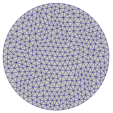
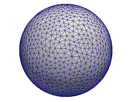
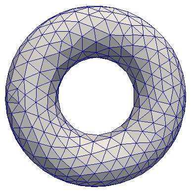
Figure 7: Sample coarse meshes of the unstructured meshes used for the 2D and 3D FEM.

In Table 1, we identify each matrix by its discretization type, spatial dimension, geometry, etc. In particular, the first letter indicates the discretization methods, where E stands for FEM and D for finite difference methods (FDM). It is then followed by the dimension (2 or 3) of the geometry. The next lower-case letter indicates different types of domains, where d stands for disk, s for sphere, t for torus, q for square, and c for cube. If different mesh sizes of the same problems were used, we append a digit to the matrix ID, where a larger digit corresponds to a finer mesh. The condition numbers are in 1-norm, estimated using MATLAB’s condest function.

5.2 Verification of Linear Complexity

For all of our test matrices, the number of nonzeros per row and per column is bounded by a constant. This is typical for linear systems from PDE discretization methods that use compact local stencils. Hence, their computational cost should ideally be linear in the number of unknowns. To verify the complexity analysis in Proposition 2, we consider matrices E2d1–7 from FEM 2D, whose unknowns range between approximately $37$K and $450$K, as well as E3s1–6 from FEM 3D, whose unknowns range between approximately $26$K and $386$K unknowns. Figure 8 shows the scalability plots of the overall factorization time for FEM 2D (left) and 3D (right), respectively. The x-axis corresponds to the number of unknowns, and the y-axis corresponds to the normalized costs, both in logarithmic scale. For PS-MILU, we show both the estimated floating-point operations in level-1, along with the overall computational cost at all levels, including the preprocessing steps. We used the default tolerances as in Figure 6. As references, we also plot the costs for multilevel ILU in ILUPACK v2.4 [11] and supernodal ILU in SuperLU v5.2.1 [29] for these systems, both with their respective default parameters. All the tests were conducted in serial on a single node of a cluster with two 2.5 GHz Intel Xeon CPU E5-2680v3 processors and 64 GB of memory. For accurate timing, both turbo and power saving modes were turned off for the processors, and each node was dedicated to run one problem at a time. Since the implementations may have a significant impact on the actual runtime, we normalize each of these measures by dividing it by its corresponding measure for the coarsest mesh.

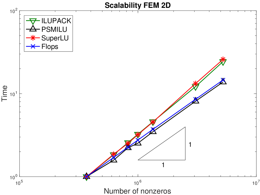
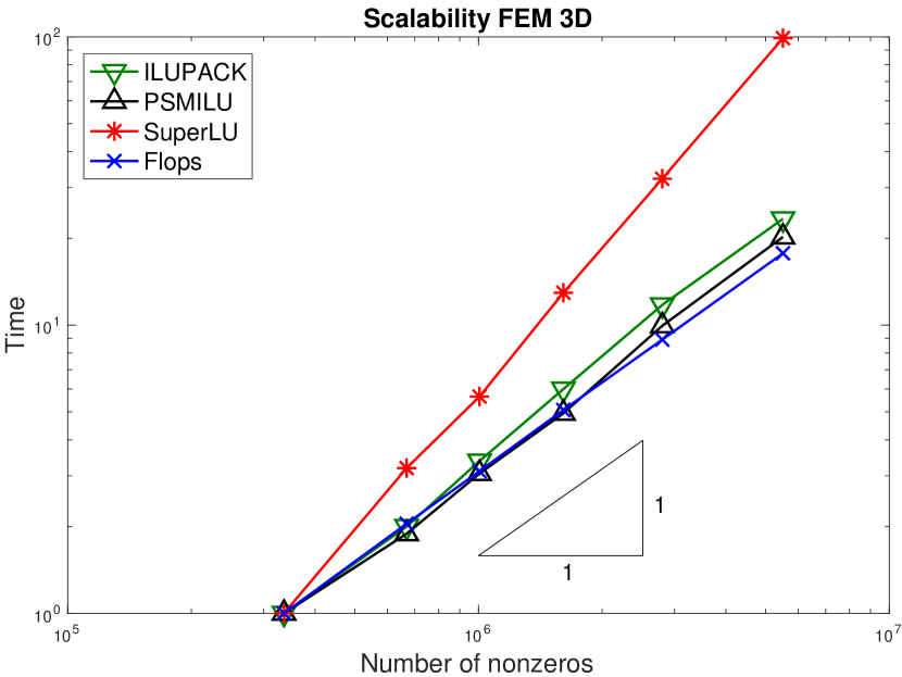
Figure 8: Asymptotic growth of factorization times of E2d1–7 (left) and E3s1–6 with PS-MILU along with ILUPACK and SuperLU, compared against theoretical flop counts.

In Figure 8, it can be seen that the total number of floating-point operations in level-1 scales linearly, as predicted by Proposition 2. Since the updates in level-1 dominate the overall algorithm, PS-MILU exhibited almost linear scaling overall, despite nearly quadratic cost of the pre-processing steps. In contrast, the supernodal ILU in SuperLU scales superlinearly, and has much higher complexities in 3D than 2D. This is primarily due to the use of column pivoting in SuperLU. On the other hand, ILUPACK scales much worse than PS-MILU in 2D, at a rate comparable with SuperLU, although it scales nearly as good as PS-MILU for 3D problems. This is because the condition numbers of the linear systems from Poisson equations grow at the rate of $\mathcal{O}(h^{-2})$, where $h$ denotes the average edge length for quasi-uniform meshes. In 2D and 3D, the condition numbers are approximately $\mathcal{O}(n)$ and $\mathcal{O}(n^{2/3})$, respectively. Hence, with similar numbers of unknowns, 2D problems tend to lead to more pivoting and more levels with multilevel ILU. Because ILUPACK switches to use the T-version of the Schur complements when the number of levels is large, it suffered from higher time complexities for 2D problems than 3D problems. PS-MILU overcomes their scalability issues by using diagonal pivoting instead of column pivoting and using the H-version only for constant-size Schur complements.

5.3 Speedup due to Predominant Symmetry

In Table 1, due to the surface-to-volume ratio, the symmetric portions of these systems are predominant. PS-MILU may speed up the factorization by a factor of $2$ for the update of $\boldsymbol{L}_{B}$ and $\boldsymbol{U}_{B}$ by utilizing symmetry. However, since both $\boldsymbol{L}_{E}$ and $\boldsymbol{U}_{F}$ must be updated in PS-MILU, we cannot expect a perfect twofold speedup. Table 2 compares the speedups of PS-MILU versus nonsymmetric MILU at level 1 for 14 matrices. We show both the speedups of Crout update alone and those of the overall factorization step. The Crout update achieved a nearly twofold speedup for most cases, and the overall factorization achieved a speedup between 1.4 and $1.6$.

Table 2: Speedups of PS-MILU versus nonsymmetric MILU by taking advantage of predominant symmetry at level 1.

Matrix ID	Update Speedup	Overall Speedup
E2d4	1.8	1.5
E2d5	1.9	1.5
E2d6	1.8	1.5
E2d7	1.8	1.5
E3s4	1.8	1.5
E3s5	1.9	1.6
E3s6	1.8	1.6
E3t1	1.7	1.5
E3t2	1.7	1.5
E3t3	1.7	1.5
D2q1	1.7	1.4
D2q2	1.7	1.4
D3c1	1.9	1.5
D3c2	1.9	1.5

5.4 Effectiveness as Preconditioners

Finally, we assess the effectiveness of PS-MILU as a preconditioner. In particular, we compare PS-MILU versus using the fully nonsymmetric MILU as a right-preconditioner of GMRES(30) for solving predominantly symmetric systems. Table 4 shows the ratios of the numbers of nonzeros in the output versus that in the input (i.e., $\text{nnz}(\boldsymbol{L}+\boldsymbol{D}+\boldsymbol{U})/\text{nnz}(\boldsymbol{A})$), the number of diagonal pivots, and the number of GMRES iterations for both nonsymmetric MILU and PS-MILU. Our default thresholds in the previous subsection worked for all of the test problems. In Table 4, we used the default drop-tolerances for most problems. For the well-conditioned E3s1-6 and D3c1-2, there was no pivoting with the default parameters, so we used $\tau_{k}=20$ to force some pivoting. It appeared that nonsymmetric MILU is more sensitive to the thresholds than PS-MILU, in that a smaller $\tau_{k}$ tends to lead to more pivoting for nonsymmetric MILU than for PS-MILU.

Table 3: Comparison of PS-MILU versus nonsymmetric MILU as a right-preconditioner for GMRES(30). In the GMRES columns, the numbers in each entry are the numbers of iterations with relative convergence tolerances of $10^{-6}$ and $10^{-12}$, respectively

Matrix	nonsymmetric MILU			PS-MILU
	Ratio	#Pivots	GMRES	Ratio	#Pivots	GMRES
E2d4	2.00	430	59/128	2.01	401	59/123
E2d5	2.01	613	63/157	2.07	555	63/158
E2d6	2.01	1447	113/305	2.09	1335	111/299
E2d7	2.00	2503	145/410	2.09	2302	144/404
E3s4	2.26	476	16/37	2.33	450	16/38
E3s5	2.28	1005	17/44	2.34	728	17/46
E3s6	2.31	2213	19/55	2.38	1543	20/57
E3t1	2.27	123	34/97	2.21	71	25/67
E3t2	2.28	167	35/108	2.26	110	30/88
E3t3	2.33	270	60/166	2.32	199	42/124
D2q1	3.58	468	72/203	3.81	345	72/204
D2q2	3.58	600	109/282	3.77	623	112/295
D3c1	4.41	652	21/41	4.56	411	21/41
D3c2	4.45	1188	25/51	4.60	844	26/52

To assess the robustness of PS-MILU as a preconditioner, we use a relative convergence tolerance of $10^{-12}$ for GEMRES(30). It is well known that the restarted GEMRES tends to stagnate for large systems without a good preconditioner. However, GMRES(30) with PS-MILU succeeded for all of our test cases for such a small tolerance. Since some software (such as MATLAB) use $10^{-6}$ as the default convergence tolerance for GMRES, we report the numbers of iterations of GMRES(30) to achieve both $10^{-6}$ and $10^{-12}$. It can be seen that PS-MILU and MILU produced comparable numbers of nonzeros and GMRES iterations for most cases. However, nonsymmetric MILU tends to introduce more pivots. In addition, PS-MILU accelerated the convergence of GMRES better than nonsymmetric MILU for E3t1–3, which are the most ill-conditioned linear systems in our tests. Note that the number of iterations more than doubled when squaring the convergence tolerance, indicating a sub-linear convergence rate of GMRES(30) due to restarts. In addition, the number of iterations still grew as the problem size increased. We observed the same behavior with ILUPACK. Hence, in spite of the linear complexity PS-MILU, one cannot expect the overall time complexity to be linear when using PS-MILU as a preconditioner of a Krylov subspace method. For a truly scalable solver, one would still need to use multigrid methods.

6 Conclusions and Future Work

In this paper, we proposed a multilevel incomplete LU factorization technique, called PS-MILU, as a preconditioner for Krylov subspace methods. PS-MILU unifies the treatment of symmetric and nonsymmetric linear systems, and it is robust due to the use of scaling, diagonal pivoting, inverse-based thresholding, and systematic treatment of the Schur complement. Its computational cost is nearly linear in the number of unknowns for typical linear systems arising from PDE discretizations. This is achieved by introducing augmented CCS and CRS data structures and conducting careful complexity analysis of the algorithm. In addition, we also introduced the concept of predominantly symmetric matrices. We showed that PS-MILU can take advantage of this partial symmetry to speed up the update operations by nearly a factor of two. We have implemented the proposed algorithm in MATLAB and reported numerical experimentation to demonstrate its robustness and linear scaling for a collection of benchmark problems with up to half a million unknowns. In addition, we compared PS-MILU against multilevel ILU in ILUPACK and the supernodal ILU and analyzed the reasons of their poor scaling, and explained how PS-MILU avoided those issues.

There are several limitations in this work. First, we primarily considered linear systems from PDE discretizations. Although we have tested the robustness of PS-MILU for smaller benchmark problems from other domains in the literature, we have not assessed the scalability for large systems from other applications, such as large KKT systems arising from constrained optimizations. Second, we only considered MC64 matching during preprocessing. There are other preprocessing techniques, such as PQ-reordering [35], which may be beneficial for PS-MILU. Third, our current algorithm is only sequential, which will ultimately limit the sizes of the problems that can be solved. Finally, our proof-of-concept implementation is in MATLAB, which is not the most efficient. We plan to address these issues in our future research.

References

- [1] P. R. Amestoy, T. A. Davis, and I. S. Duff. An approximate minimum degree ordering algorithm. SIAM J. Matrix Anal. Appl., 17(4):886–905, 1996.
- [2] S. Balay, S. Abhyankar, M. F. Adams, J. Brown, P. Brune, K. Buschelman, L. Dalcin, V. Eijkhout, W. D. Gropp, D. Kaushik, M. G. Knepley, L. C. McInnes, K. Rupp, B. F. Smith, S. Zampini, and H. Zhang. PETSc Users Manual. Technical Report ANL-95/11 - Revision 3.7, Argonne National Laboratory, 2016.
- [3] M. Benzi, G. H. Golub, and J. Liesen. Numerical solution of saddle point problems. Acta Numerica, 14:1–137, 5 2005.
- [4] M. Benzi, J. C. Haws, and M. Tuma. Preconditioning highly indefinite and nonsymmetric matrices. SIAM J. Sci. Comput., 22(4):1333–1353, 2000.
- [5] P. Bochev, J. Cheung, M. Perego, and M. Gunzburger. Optimally accurate higher-order finite element methods on polytopial approximations of domains with smooth boundaries. arXiv preprint arXiv:1710.05628, 2017.
- [6] R. F. Boisvert, R. Pozo, K. Remington, R. F. Barrett, and J. J. Dongarra. Matrix Market: a web resource for test matrix collections. In Qual. Numer. Softw., pages 125–137. Springer, 1997.
- [7] M. Bollhöfer. A robust and efficient ILU that incorporates the growth of the inverse triangular factors. SIAM J. Sci. Comput., 25(1):86–103, 2003.
- [8] M. Bollhöfer, J. I. Aliaga, A. F. Martın, and E. S. Quintana-Ortí. ILUPACK. In Encyclopedia of Parallel Computing. Springer, 2011.
- [9] M. Bollhöfer and Y. Saad. On the relations between ILUs and factored approximate inverses. SIAM J. Matrix Anal. Appl., 24(1):219–237, 2002.
- [10] M. Bollhöfer and Y. Saad. Multilevel preconditioners constructed from inverse-based ILUs. SIAM J. Sci. Comput., 27(5):1627–1650, 2006.
- [11] M. Bollhöfer and Y. Saad. ILUPACK preconditioning software package. Available online at http://ilupack.tu-bs.de/. Release V2.4, June., 2011.
- [12] J. R. Bunch and B. N. Parlett. Direct methods for solving symmetric indefinite systems of linear equations. SIAM J. Num. Anal., 8(4):639–655, 1971.
- [13] T. F. Chan, E. Gallopoulos, V. Simoncini, T. Szeto, and C. H. Tong. A quasi-minimal residual variant of the Bi-CGSTAB algorithm for nonsymmetric systems. SIAM J. Sci. Comput., 15(2):338–347, 1994.
- [14] T. F. Chan and H. A. Van Der Vorst. Approximate and incomplete factorizations. In Parallel Numerical Algorithms, pages 167–202. Springer, 1997.
- [15] E. Chow and A. Patel. Fine-grained parallel incomplete LU factorization. SIAM J. Sci. Comput., 37(2):C169–C193, 2015.
- [16] A. K. Cline, C. B. Moler, G. W. Stewart, and J. H. Wilkinson. An estimate for the condition number of a matrix. SIAM J. Num. Anal., 16(2):368–375, 1979.
- [17] T. A. Davis and Y. Hu. The University of Florida sparse matrix collection. ACM Trans. Math. Softw., 38(1):1, 2011.
- [18] I. S. Duff and J. Koster. The design and use of algorithms for permuting large entries to the diagonal of sparse matrices. SIAM J. Matrix Anal. Appl., 20(4):889–901, 1999.
- [19] T. Dupont, R. P. Kendall, and H. Rachford, Jr. An approximate factorization procedure for solving self-adjoint elliptic difference equations. SIAM J. Num. Anal., 5(3):559–573, 1968.
- [20] R. W. Freund. A transpose-free quasi-minimal residual algorithm for non-Hermitian linear systems. SIAM J. Sci. Comput., 14(2):470–482, 1993.
- [21] M. Gee, C. Siefert, J. Hu, R. Tuminaro, and M. Sala. ML 5.0 smoothed aggregation user’s guide. Technical Report SAND2006-2649, Sandia National Laboratories, Albuquerque, NM, 2006.
- [22] A. George and J. W. Liu. Computer solution of large sparse positive definite systems. Prentice-Hall, Englwood Cliffs. NJ, 1981.
- [23] C. Geuzaine and J.-F. Remacle. Gmsh: a three-dimensional finite element mesh generator with built-in pre- and post-processing facilities. Int. J. Numer. Meth. Engrg., 79(11):1309–1331, 2009.
- [24] A. Ghai, C. Lu, and X. Jiao. A comparison of preconditioned krylov subspace methods for large-scale nonsymmetric linear systems. Numer. Linear Algebra Appl., page e2215, 2017.
- [25] G. H. Golub and C. F. Van Loan. Matrix Computations, volume 3. JHU Press, 2012.
- [26] I. Gustafsson. A class of first order factorization methods. BIT Numerical Mathematics, 18(2):142–156, 1978.
- [27] P. Heggernes, S. Eisenstat, G. Kumfert, and A. Pothen. The computational complexity of the minimum degree algorithm. In Proceedings of 14th Norwegian Computer Science Conference, pages 98–109, 2001.
- [28] N. Li, Y. Saad, and E. Chow. Crout versions of ILU for general sparse matrices. SIAM J. Sci. Comput., 25(2):716–728, 2003.
- [29] X. S. Li. An overview of SuperLU: Algorithms, implementation, and user interface. ACM Trans. Math. Softw., 31(3):302–325, 2005.
- [30] X. S. Li and M. Shao. A supernodal approach to incomplete LU factorization with partial pivoting. ACM Trans. Math. Softw., 37(4), 2010.
- [31] M. Olschowka and A. Neumaier. A new pivoting strategy for Gaussian elimination. Linear Algebra Appl., 240:131–151, 1996.
- [32] Y. Saad. ILUT: A dual threshold incomplete LU factorization. Numer. Linear Algebra Appl., 1, 1994.
- [33] Y. Saad. Sparsekit: a basic toolkit for sparse matrix computations. Technical report, University of Minnesota, 1994.
- [34] Y. Saad. Iterative Methods for Sparse Linear Systems. SIAM, 2nd edition, 2003.
- [35] Y. Saad. Multilevel ILU with reorderings for diagonal dominance. SIAM J. Sci. Comput., 27(3):1032–1057, 2005.
- [36] Y. Saad and M. Schultz. GMRES: A generalized minimal residual algorithm for solving nonsymmetric linear systems. SIAM J. Sci. Stat. Comput., 7(3):856–869, 1986.
- [37] H. D. Simon et al. Incomplete LU preconditioners for conjugate-gradient-type iterative methods. SPE Reservoir Engineering, 3(01):302–306, 1988.
- [38] The HYPRE Team. hypre High-Performance Preconditioners User’s Manual, 2017. version 2.12.2.
- [39] The MathWorks, Inc. MATLAB R2017a. Natick, MA, 2017. http://www.mathworks.com/.
- [40] M. Tismenetsky. A new preconditioning technique for solving large sparse linear systems. Linear Algebra Appl., 154(331–353), 1991.
- [41] H. A. van der Vorst. Bi-CGSTAB: A fast and smoothly converging variant of Bi-CG for the solution of nonsymmetric linear systems. SIAM J. Sci. Stat. Comput., 13(2):631–644, 1992.