SalSi: A new seismic attribute for salt dome detection

Abstract

In this paper, we propose a saliency-based attribute, SalSi, to detect salt dome bodies within seismic volumes. SalSi is based on the saliency theory and modeling of the human vision system (HVS). In this work, we aim to highlight the parts of the seismic volume that receive highest attention from the human interpreter, and based on the salient features of a seismic image, we detect the salt domes. Experimental results show the effectiveness of SalSi on the real seismic dataset acquired from the North Sea, F3 block. Subjectively, we have used the ground truth and the output of different salt dome delineation algorithms to validate the results of SalSi. For the objective evaluation of results, we have used the receiver operating characteristics (ROC) curves and area under the curves (AUC) to demonstrate SalSi is a promising and an effective attribute for seismic interpretation.

Index Terms—  Saliency, Seismic attribute, Salt dome detection, SalSi, Seismic interpretation.

1 Introduction

The deposition of salt may penetrate into surrounding rock strata such as limestone and shale to form an important diapir structure, a salt dome. Salt, which is impermeable, forms domes that trap hydrocarbon materials including petroleum and natural gas. Therefore, locating salt domes is key to exploring oil and petroleum reservoirs. Experienced interpreters can manually label the boundaries of salt domes by observing and analyzing seismic signals. With the dramatically growing size of acquired seismic data, however, manual labeling of the salt domes is becoming very time consuming and labor intensive. To improve interpretation effectiveness, in recent decades, both industry and academia have used intelligent computer-aided methods to assist the interpretation process. Salt dome delineation, however, poses significant detection and labeling problems because of noise and amplitude variations in seismic data. Fully and semi-automated interpretation algorithms are usually applied to 2D seismic sections to detect an initial boundary of the salt body. Interpreters, based on an initial output, can fix the erroneously detected boundary sections and fine tune the algorithm’s parameters to accurately segment salt domes. In this context, having a confidence region around salt dome for delineating boundary and fine tune certain parameters can enhance algorithm’s efficiency, reduce computational complexity and speed up the interpretation process.

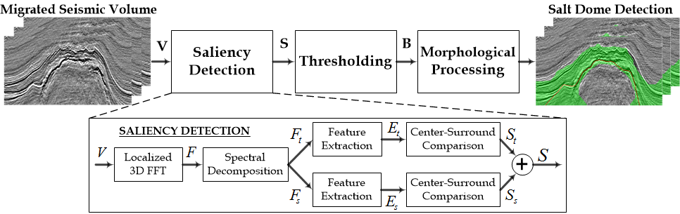
Fig. 1: Block diagram of the proposed method

Researchers, over the last few decades, have proposed several subsurface structures detection methods based on the visual perception of interpreters. In particular, there are several works on the detection of salt domes using graph theory, edge detection, texture, normalized graph cut, active contours and different image processing techniques [1, 2, 3, 4, 5, 6, 7, 8, 9, 10, 11, 12, 13]. One of the rarely explored descriptor for seismic interpretation is saliency. Drissi et al. [14] proposed an algorithm to detect the salient texture features in seismic sections by computing entropy at each pixel using two entropy measures: the Shannon entropy and the generalized cumulative residual entropy. Visual saliency is important to predict the human interpreters attention and highlight the areas of interest in seismic sections. However, the majority of algorithms haven’t exploited visual saliency for salt dome detection and seismic interpretation.

Saliency detection aims to highlight salient regions in images and videos by taking into consideration the biological structure of the human vision system (HVS) [15]. As a great deal of research in computational cognitive science suggests, HVS has evolved to reduce the amount of the sensory data information gathering stage, also known as the task-free visual search, by focusing on the perceptually salient segments of visual data that conveys the most useful information about the scene [16]. Features like color contrast, intensity contrast, flicker, and motion all have been identified as prominent features that help HVS to focus processing resources on important elements in the surrounding environment. One of the most widely accepted theories to characterize saliency and HVS states that localized outliers in both temporal and spatial domains represent novel elements in the environment. The computational aspect of this theory is structured into the center-surround model [17], in which a saliency map can be obtained by comparing regions in the visual input to its local surrounding in terms of visual feature that have been identified as saliency prominent. Several features and detection algorithms for saliency have been proposed in the literature [15, 16]. More recently, a 3D Fast Fourier Transform (FFT)-based saliency detection algorithm for video has been proposed [18]. This algorithm uses 3D FFT of a non-overlapping window in the spatial and temporal domains of video sequence to compute the spectral energy of the window and compare it with its surrounding regions to construct the saliency map. This method is effective in capturing both temporal and spatial saliency cues in a very fast and compact way. Therefore, we base our research in this paper on the 3D FFT-based saliency detection algorithm.

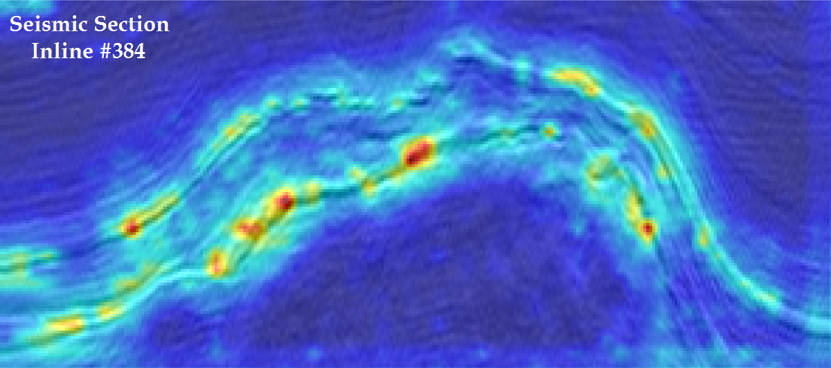
Fig. 2: Saliency map superimposed on the seismic section inline #384

In this paper, we propose a novel saliency-based attribute, SalSi. To the best of our knowledge, saliency-based salt dome detection is not reported in the literature. Using SalSi, we can process visual stimuli in real-time and perform complex processing procedures faster and more efficiently. The rest of the paper is organized as follows. The proposed salt dome detection method is given in section II. The discussion of experimental results is presented in section III, and finally conclusions are given in section IV.

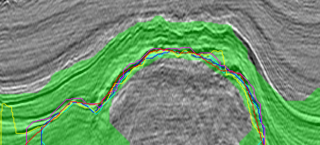
(a) Seismic section inline $\#$369

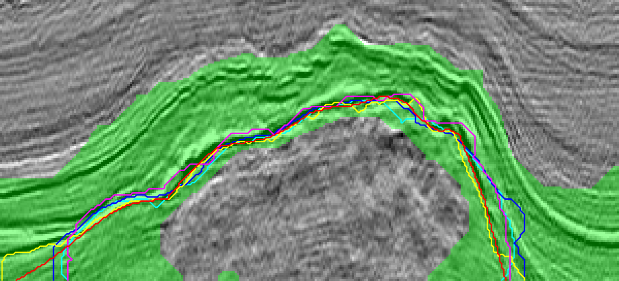
(b) Seismic section inline $\#$384

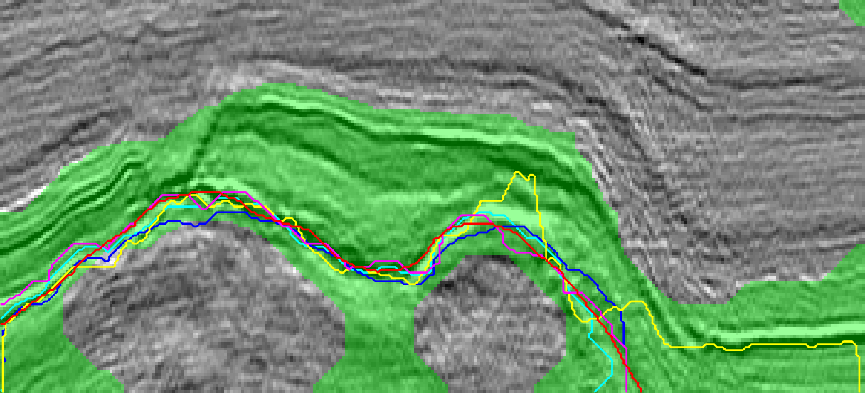
(c) Seismic section inline $\#$429

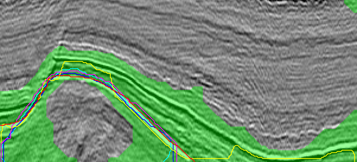
(d) Seismic section inline $\#$459

Fig. 3: Experimental results: SalSi output superimposed on different seismic sections. Magenta: Aqrawi et al. [6], Yellow: Berthelot et al. [11], Cyan: Zhen et al. [12], Blue: Shafiq et al. [13], Green: SalSi Output, Red: Ground Truth.

2 Proposed Method for Salt Dome Detection

An overall block diagram of SalSi is shown in Fig. 1. For the application under consideration, the most salient part of a seismic image is salt dome boundary. Thus, given a 3D seismic data volume $\boldsymbol{V}$ of size $M\times N\times K$, where $M$ represents time depth, $N$ represents crosslines and $K$ represents inlines, we compute saliency using the 3D FFT-based algorithm proposed in [18]. The 3D FFT-based saliency algorithm is fast, and obtains saliency maps with adjustable resolution, that allows better salient objects segmentation. The 3D FFT-based algorithm is computationally inexpensive and requires very few parameters as compared to other visual saliency algorithms, which make it advantageous for seismic applications. The block diagram of 3D FFT-based saliency detection algorithm is also shown in Fig. 1.

To perform the saliency detection, first we calculate the 3D FFT spectrum $\boldsymbol{F}$ in a local area using (1), and decompose $\boldsymbol{F}$ into a temporal-change-related component $\boldsymbol{F}_{t}$ and a spatial-change-related component $\boldsymbol{F}_{s}$.

$$F[u,v,w]=\frac{1}{L^{3}}\sum\limits_{m=0}^{L-1}\sum\limits_{n=0}^{L-1}\sum\limits_{k=0}^{L-1}f[m,n,k]e^{-2\pi i\left(mu+nv+kw\right)/L},$$ (1)

$$F_{t}[u,v,w]=F[u,v,w]\times\frac{w}{\sqrt[]{u^{2}+v^{2}+w^{2}}},$$ (2)

$$F_{s}[u,v,w]=F[u,v,w]\times\frac{\sqrt[]{u^{2}+v^{2}}}{\sqrt[]{u^{2}+v^{2}+w^{2}}},$$ (3)

where $[m,n,k]$ and $[u,v,w]$ represent the coordinates in the space and frequency domains, respectively, $L$ defines the size of the local data cube, and $f[m,n,k]$ is the seismic image or section. Subsequently, spectral energies $\boldsymbol{E}_{t}$ and $\boldsymbol{E}_{s}$ are extracted from $\boldsymbol{F}_{t}$ and $\boldsymbol{F}_{s}$, respectively, as features. Applying the center-surround model, two saliency maps $\boldsymbol{S}_{t}$ and $\boldsymbol{S}_{s}$ can be constructed using $\boldsymbol{E}_{t}$ and $\boldsymbol{E}_{s}$ as

$$S_{x}[m,n,k]= \frac{1}{Q}\sum_{i_{0},j_{0},r_{0}}|E_{x}[m,n,k]$$

$$-E_{x}[m+i_{0},n+j_{0},k+r_{0}]|,$$ (4)

where $i_{0}$, $j_{0}$, $r_{0}$ are chosen such that point $[m+i_{0},n+j_{0},k+r_{0}]$ is in the immediate neighborhood of point $[m,n,k]$, such as within a $3\times 3\times 3$ window centered at $[m,n,k]$, $Q$ is the total number of points included in the summation, $\boldsymbol{S}_{x}$ represents $\boldsymbol{S}_{t}$ or $\boldsymbol{S}_{s}$, and $\boldsymbol{E}_{x}$ represents $\boldsymbol{E}_{t}$ or $\boldsymbol{E}_{s}$. The final saliency map $\boldsymbol{S}$ is obtained by averaging $\boldsymbol{S}_{t}$ and $\boldsymbol{S}_{s}$, and is of same size as of $\boldsymbol{V}$.

$$S[m,n,k]=0.5\times S_{t}[m,n,k]+0.5\times S_{s}[m,n,k].$$ (5)

The second step of SalSi is to threshold the saliency map, $\boldsymbol{S}$ as in (6).

$$\mathbf{B}[m,n,k]=\left\{\begin{aligned} &1\quad\mathbf{S}[m,n,k]\geq\mathbf{T}\\ &0\quad\mbox{Otherwise}\end{aligned}\right.,$$ (6)

where $\mathbf{B}$ represents the binary volume and white regions in $\mathbf{B}$ will likely contain salt dome boundaries. We calculate the threshold value, $\mathbf{T}$, using Otsu’s method [19]. In contrast to the non-salt regions, salt dome boundaries commonly have higher $\boldsymbol{S}$ values. Therefore, we assume that the histogram of volume $\boldsymbol{S}$ follows a bi-modal distribution shape. To optimally divide all points into two classes, we determine the threshold $T$ by minimizing the intra-class variance as follows:

$$\arg\underset{T}{\min}\left\{\sigma_{1}^{2}(T)\sum_{i=0}^{T-1}p(i)+\sigma_{2}^{2}(T)\sum_{i=T}^{H}p(i)\right\},$$ (7)

where $H$ is the number of quantized gray-levels of $\boldsymbol{S}$, and $p(i)$, $i=0,\cdots,H-1$, represents the probability of points with gray value $i$. In addition, $\sigma_{1}^{2}$ and $\sigma_{2}^{2}$ define the individual class variances, which can be calculated as follows:

$$\left\{\begin{aligned} &\sigma_{1}^{2}=\sum\limits_{i=0}^{T-1}\left[i-\sum\limits_{i=0}^{T-1}\frac{iP(i)}{P_{1}}\right]^{2}\frac{P(i)}{P_{1}},\quad P_{1}=\sum\limits_{i=0}^{T-1}P(i)\\ &\sigma_{2}^{2}=\sum\limits_{i=T}^{H-1}\left[i-\sum\limits_{i=T}^{H-1}\frac{iP(i)}{P_{2}}\right]^{2}\frac{P(i)}{P_{2}},\quad P_{2}=\sum\limits_{i=T}^{H-1}P(i)\\ \end{aligned}\right.$$ (8)

Therefore, on the basis of (7), we can adaptively identify threshold $T$ by exhaustively searching between $0$ and $H-1$.

Salt domes are complicated structures and after applying the threshold $\boldsymbol{T}$ on $\boldsymbol{S}$, it is inevitable that the binary volume $\boldsymbol{B}$ contains noisy or disconnected boundary regions. In order to process noisy and disconnected boundary regions, finally we apply morphological closing operation as a post processing step to $\boldsymbol{B}$ to ensure salt body is closed. In morphological closing operation, which is comprised of dilation followed by erosion, we have used circular disk of radius ten as structuring element $\boldsymbol{Se}$. As a result of morphological operation, SalSi will generate a salient map of a seismic image that highlights the salt dome boundary.

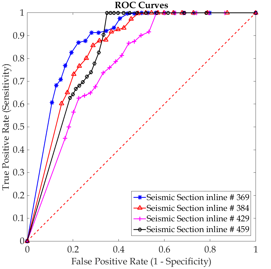
Fig. 4: ROC curves

3 Experimental Results

In this section, we present the effectiveness of SalSi for salt dome detection. We have used the real seismic dataset acquired from the Netherland’s offshore, $F3$ block in the North Sea, whose size is $24$ x $16$ $km^{2}$ [20]. The seismic volume that contains the salt dome structure has an inline number ranging from $\#151$ to $\#501$, a crossline number ranging from $\#401$ to $\#701$, and a time direction ranging from $1,300ms$ to $1,848ms$ sampled every $4ms$.

A typical seismic section’s saliency map superimposed on original image is shown in Fig. 2. It can be observed from Fig. 2 that the saliency map depicts boundary at the salt dome perimeter. The output of SalSi, and the results of different salt dome delineation algorithms on seismic section inlines #369, #384, #429 and #459 are shown in Fig. 3, with the ground truth manually labeled in red. The magenta, yellow, cyan and blue lines represent the boundaries detected by [6], [11], [12] and [13], respectively, whereas the green area represents SalSi output. Subjectively, it can be observed that the boundaries detected by all aforementioned algorithms lie within SalSi output, which make it suitable for algorithms initialization, tracking boundaries within seismic volumes, and reducing time computation.

To objectively evaluate the effectiveness of SalSi with different thresholds, we calculated the receiver operating characteristics (ROC) curves, and the area under the curve (AUC) of different seismic section inlines. We used multi-level threshold [21] and measured SalSi performance using two important statistical measures, sensitivity and specificity, usually used in binary classification. Sensitivity, which is also called true positive rate (TPR) measures the voxels that are correctly identified using SalSi. On the other hand, specificity, also known as true negative rate measures the proportion of voxels that don’t belong to the salt dome boundary and are correctly identified as such. Fall out rate also termed at false positive rate or false alarm can be calculated as (1-specificity). ROC curves, obtained by plotting sensitivity against fall out rate, are shown in Fig. 4. These curves illustrates the performance of SalSi as a binary classifier when threshold is varied between a certain range. A good detection method has ROC curve over the random selection method, depicted by dashed red line in Fig. 4, and it can be observed that all ROC curves of SalSi are above random selection method. An optimum threshold can also be obtained by averaging all ROC curves and comparing TPR with FPR. A good threshold value will generate a saliency map with maximum sensitivity and minimum fall out rate. We also calculated the AUC values from the ROC curves, and results are presented in Table. 1. The AUC values closer to one indicate that the detection method is very good and Table. 1 demonstrates that SalSi performs very well on different seismic section inlines and has mean AUC of 0.8324. Therefore, experimental results presented in this paper show a promising future of SalSi for salt dome detection and very good potential for seismic interpretation.

Table 1: The AUC values of the ROC curves

Sr. $\#$	Seismic Section	AUC
1	Inline $\#$ 369	0.8803
2	Inline $\#$ 384	0.8434
3	Inline $\#$ 429	0.7740
4	Inline $\#$ 459	0.8317

4 Conclusion

In this paper, we have proposed a novel saliency-based attribute, SalSi, for salt dome detection from seismic volumes. SalSi can be used to initialize algorithms and to reduce computational complexity of algorithms. Therefore, SalSi is also suitable for many seismic interpretation applications such as salt dome delineation, tracking salt domes in seismic volume, seismic retrieval and labeling, etc. SalSi, originally designed to detect salt domes can be modified to capture chaotic horizons and faults as well from seismic volumes. The experimental results show that SalSi can accurately locate salt domes within seismic volumes and enhance the efficiency of interpretation process. The AUC and ROC curves demonstrate that SalSi performs very well even with the different threshold values, which validate SalSi as an effective attribute for seismic interpretation. Initial results of SalSi presented in this paper are very encouraging having various applications in seismic interpretation.

References

- [1] Jesse Lomask, Biondo Biondi, and Jeff Shragge, “Image segmentation for tracking salt boundaries,” in Expanded Abstracts of the SEG 74th Annual Meeting, 2004, pp. 2443–2446.
- [2] Jesse Lomask, Robert G. Clapp, and Biondo Biondi, “Application of image segmentation to tracking 3D salt boundaries,” Geophysics, vol. 72, no. 4, pp. P47–P56, 2007.
- [3] Jianbo Shi and Jitendra Malik, “Normalized cuts and image segmentation,” Pattern Analysis and Machine Intelligence, IEEE Transactions on, vol. 22, no. 8, pp. 888–905, 2000.
- [4] Adam D. Halpert, Robert G. Clapp, and Biondo Biondi, “Seismic image segmentation with multiple attributes,” in Expanded Abstracts of the SEG 79th Annual Meeting. Society of Exploration Geophysicists, 2009, pp. 3700–3704.
- [5] Jing Zhou, Yanqing Zhang, Zhigang Chen, and Jianhua Li, “Detecting boundary of salt dome in seismic data with edge detection technique,” in Expanded Abstracts of the SEG 77th Annual Meeting. Society of Exploration Geophysicists, 2007, pp. 1392–1396.
- [6] Ahmed Adnan Aqrawi, Trond Hellem Boe, and Sergio Barros, “Detecting salt domes using a dip guided 3D Sobel seismic attribute,” in Expanded Abstracts of the SEG 81st Annual Meeting. Society of Exploration Geophysicists, 2011, pp. 1014–1018.
- [7] Asjad Amin and Mohamed Deriche, “A new approach for salt dome detection using a 3d multidirectional edge detector,” Applied Geophysics, vol. 12, no. 3, pp. 334–342, 2015.
- [8] M. Shafiq, Z. Wang, and G. AlRegib, “Seismic interpretation of migrated data using edge-based geodesic active contours,” in Proc. IEEE Global Conf. on Signal and Information Processing (GlobalSIP), Orlando, Florida, Dec. 14-16, 2015.
- [9] Jarle Haukas, Oda Roaldsdotter Ravndal, Bjorn Harald Fotland, Aicha Bounaim, and Lars Sonneland, “Automated salt body extraction from seismic data using level set method,” First Break, EAGE, vol. 31, Apr 2013.
- [10] Winston Lewis, Bill Starr, and Denes Vigh, “A level set approach to salt geometry inversion in full-waveform inversion,” SEG Las Vegas 2012 Annual Meeting, 2012.
- [11] Angélique Berthelot, Anne HS Solberg, and Leiv J. Gelius, “Texture attributes for detection of salt,” Journal of Applied Geophysics, vol. 88, pp. 52–69, 2013.
- [12] Zhen Wang, Tamir Hegazy, Zhiling Long, and Ghassan AlRegib, “Noise-robust detection and tracking of salt domes in postmigrated volumes using texture, tensors, and subspace learning,” Geophysics, vol. 80, no. 6, pp. WD101–WD116, 2015.
- [13] Muhammad A. Shafiq, Zhen Wang, Asjad Amin, Tamir Hegazy, Mohamed Deriche, and Ghassan AlRegib, “Detection of salt-dome boundary surfaces in migrated seismic volumes using gradient of textures,” in Expanded Abstracts of the SEG 85th Annual Meeting, New Orleans, Louisiana, 2015, pp. 1811–1815.
- [14] N. Drissi, T. Chonavel, and J.M. Boucher, “Salient features in seismic images,” in OCEANS 2008 - MTS/IEEE Kobe Techno-Ocean, April 2008, pp. 1–4.
- [15] A. Borji and L. Itti, “State-of-the-art in visual attention modeling,” Pattern Analysis and Machine Intelligence, IEEE Transactions on, vol. 35, no. 1, pp. 185–207, Jan 2013.
- [16] A. Borji, “What is a salient object? a dataset and a baseline model for salient object detection,” Image Processing, IEEE Transactions on, vol. 24, no. 2, pp. 742–756, Feb 2015.
- [17] D. Gao, V. Mahadevan, and N. Vasconcelos, “On the plausibility of the discriminant center-surround hypothesis for visual saliency,” Journal of Vision, vol. 8, no. 7, pp. 1–18, 2008.
- [18] Zhiling Long and Ghassan AlRegib, “Saliency detection for videos using 3D FFT local spectra,” Proc. SPIE, vol. 9394, pp. 93941G–93941G–6, 2015.
- [19] N. Otsu, “A threshold selection method from gray-level histograms,” Systems, Man and Cybernetics, IEEE Transactions on, vol. 9, no. 1, pp. 62–66, Jan 1979.
-
[20]
dGB Earth Sciences B.V.,
“The Netherlands Offshore, The North Sea, F3 Block -
Complete,”
https://opendtect.org/osr/pmwiki.php/Main/Netherlands
OffshoreF3BlockComplete4GB. - [21] Ping sung Liao, Tse sheng Chen, and Pau choo Chung, “A fast algorithm for multilevel thresholding,” Journal of Information Science and Engineering, vol. 17, pp. 713–727, 2001.