The Mahalanobis kernel for heritability estimation in genome-wide association studies:
Fixed-effects and random-effects methods

Abstract

Linear mixed models (LMMs) are widely used for heritability estimation in genome-wide association studies (GWAS). In standard approaches to heritability estimation with LMMs, a genetic relationship matrix (GRM) must be specified. In GWAS, the GRM is frequently a correlation matrix estimated from the study population’s genotypes, which corresponds to a normalized Euclidean distance kernel. In this paper, we show that reliance on the Euclidean distance kernel contributes to several unresolved modeling inconsistencies in heritability estimation for GWAS. These inconsistencies can cause biased heritability estimates in the presence of linkage disequilibrium (LD), depending on the distribution of causal variants. We show that these biases can be resolved (at least at the modeling level) if one adopts a Mahalanobis distance-based GRM for LMM analysis. Additionally, we propose a new definition of partitioned heritability – the heritability attributable to a subset of genes or single nucleotide polymorphisms (SNPs) – using the Mahalanobis GRM, and show that it inherits many of the nice consistency properties identified in our original analysis. Partitioned heritability is a relatively new area for GWAS analysis, where inconsistency issues related to LD have previously been known to be especially pernicious.

T1Supported by NSF Grant DMS-1454817.

and

1 Introduction

Heritability is the proportion of phenotypic variance explained by genetic variance (Falconer, 1960; Lynch et al., 1998). There are many different definitions of heritability and different methods for estimating heritability from data (e.g. Haseman and Elston, 1972; Henderson, 1984; Visscher, Hill and Wray, 2008; Yang et al., 2011a; Golan, Lander and Rosset, 2014; Bulik-Sullivan et al., 2015). This paper is focused on heritability estimation methods that are related to variance components estimation methods for linear mixed models (LMMs). LMM-based methods for heritability estimation have been used since the 1950s (Henderson, 1950); additionally, over the last decade they have emerged as one of the most widely-used methods for estimating heritability with genome-wide association study (GWAS) data (Hindorff et al., 2009; Yang et al., 2010; Kang et al., 2010; Zaitlen and Kraft, 2012). However, standard approaches to heritability estimation with LMMs have some unresolved inconsistencies that are related to fundamental topics in genetics – e.g. linkage disequilibrium (LD), the distribution of causal variants, and partitioning heritability – which can lead to badly biased heritability estimates (Zaitlen and Kraft, 2012; Speed et al., 2012; Gusev et al., 2013, 2014).

LMM-based heritability methods typically require specification of a genetic relationship matrix (GRM), which measures genetic similarity between subjects in a study. The GRM may be based on familial or other information (Lange, 2003; Powell, Visscher and Goddard, 2010). In GWAS, the GRM is frequently a sample correlation matrix constructed from study participant’s trinary single nucleotide polymorphism (SNP) values, which corresponds to a Euclidean distance kernel (Yang et al., 2010; Zaitlen and Kraft, 2012). In this paper, we argue that using the Euclidean kernel is a root cause for biases in LMM heritability estimation referenced in the previous paragraph. Furthermore, we argue that if one adopts a Mahalanobis kernel-based GRM, then many of the LMM heritability biases related to LD and causal variants can be tranparently explained and resolved at the modeling level. This approach yields a modified version of LMM-based heritability, relying on the Mahalanobis GRM. We also define a natural version of partitioned heritability with the Mahalanobis GRM, which resolves some closely related inconsistency issues that have been noted for other methods for partitioning heritability (Speed et al., 2012; Gusev et al., 2013, 2014). We propose a Mahalanobis kernel-based maximum likelihood estimator for both partitioned and total heritability, and show that the estimator is consistent and asymptotically normal. Throughout the paper, numerical simulations are used to help illustrate different aspects of heritability estimation and our methodological results.

Beyond their immediate practical application for estimating heritability, the statistical arguments for the Mahalanobis kernel in this paper also address several fundamental questions about statistical modeling in modern genetics, including 1) fixed-effects vs. random-effects modeling and 2) narrow-sense vs. broad-sense heritability. Questions about fixed- and random-effects modeling have been raised repeatedly in research on heritability estimation (Gibson, 2012). Many of these questions can be summarized as follows: Should genetic effects be modeled as fixed or random quantities? To answer this question, we argue that for the Mahalanobis kernel, the fixed- and random-effects models are essentially equivalent. Furthermore, under the Mahalanobis kernel, we show that the LMM heritability coefficient can also be interpreted as a conditional variance – which we refer to as the $C$-heritability ($C$ for “conditional”) – under the corresponding fixed-effects model. This builds a link between narrow-sense (or additive) heritability, which LMM-based methods have traditionally been designed to estimate, and broad-sense heritability, which is a more model-free measure of overall heritability defined in terms of the conditional variance of a phenotype given the genotype and other specified information. By introducing $C$-heritability, total and partitioned heritabilities become special cases of a general form, and we are able to propose a unified approach for both total and partitioned heritability estimation.

The rest of this paper is organized as follows. In Section 2, we review some of the common LMM heritability estimation methods and their model assumptions. Many of the biases and inconsistencies mentioned above are essentially related to model misspecification, which is discussed in detail in Section 3. In Section 4, we introduce the Mahalanobis distance-based approach, compare it with Euclidean GRM methods, and propose Mahalanobis-based estimators for heritability and partitioned heritability; $C$-heritability is also introduced and discussed in this section. Section 5 contains additional simulation results and Section 6 contains a concluding discussion.

1.1 Related work

Recently, in independent work, Mathew, Léon and Sillanpää (2018) proposed using the Mahalanobis kernel in a similar way for heritability esitmation with GWAS data. Mathew et al.’s paper primarily focuses on empirical analysis, using both simulated and real datasets to illsutrate advantages of the Mahalanobis kernel. The present work contains more precise mathematical and statistical justification for much of the work in Mathew, Léon and Sillanpää (2018), and introduces statistical principles (e.g. $C$-heritability in Section 4) that can be extended to other targeted application areas and genetics (like partitioning heritability).

2 LMMs for heritability estimation

2.1 Additive decomposition: From GRMs to LMMs

In this section, we describe a statistical model that forms the basis for many LMM heritability methods for GWAS, (e.g. Yang et al., 2010; Zaitlen and Kraft, 2012). Let $\mathbf{y}=(y_{1},\ldots,y_{n})^{\top}\in\mathbb{R}^{n}$ be a vector of centered, real-valued outcomes, where $y_{i}$ represents the phenotypic value of individual $i$ in some population. Assume that

$$\mathbf{y}=\mathbf{g}+\boldsymbol{e}$$ (1)

can be decomposed as the sum of an additive genetic effect $\mathbf{g}=(g_{1},\ldots,g_{n})^{\top}\in\mathbb{R}^{n}$ and an uncorrelated noise vector $\boldsymbol{e}=(e_{1},\ldots,e_{n})^{\top}\in\mathbb{R}^{n}$, which may contain other non-additive genetic effects, environmental noise, and measurement error. Further assume that the data are centered, so that $\mathbb{E}(\mathbf{g})=\mathbb{E}(\boldsymbol{e})=0$, and that $\mathrm{Cov}(\mathbf{g})=\sigma^{2}_{g}K$ and $\mathrm{Cov}(\boldsymbol{e})=\sigma^{2}_{e}I$, where $\sigma^{2}_{g},\sigma^{2}_{e}\geq 0$ are genetic and environmental real-valued variance components, respectively, and $K$ is the $n\times n$ GRM.

Thus, $\mathbf{y}$ is a random vector with $\mathbb{E}(\mathbf{y})=0$ and $\mathrm{Cov}(\mathbf{y})=\sigma^{2}_{g}K+\sigma^{2}_{e}I$, which we denote by

$$\mathbf{y}\sim\mathcal{MV}(0,\sigma^{2}_{g}K+\sigma^{2}_{e}I).$$ (2)

The heritability coefficient is defined to be

$$h^{2}=\frac{\sigma^{2}_{g}}{\sigma_{g}^{2}+\sigma_{e}^{2}}.$$ (3)

This definition of heritability is often referred to as narrow-sense or additive heritability. The GRM $K$ is typically normalized so that its diagonal entries all equal 1, so that the correlation matrix for $\mathbf{y}$ is $\mathrm{Corr}(\mathbf{y})=h^{2}K+(1-h^{2})I$ and the heritability parameter $h^{2}$ represents the extent to which correlation between phenotypes in the population is determined by genetic relatedness.

With GWAS data, genetic relatedness can be encoded by similarities between sequences of SNPs. Let $\mathbf{z}_{i}=(z_{i1},\ldots,z_{im})^{\top}$ be the vector of normalized SNPs for the $i$-th study subject, i.e.

$$z_{ij}=\frac{f_{ij}-2p_{j}}{\sqrt{2p_{j}(1-p_{j})}},$$

where $f_{ij}=0,1,2$ is the minor allele count at SNP $j$ for individual $i$ and $p_{j}$ is the minor allele frequency (MAF) of SNP $j$ across the population (Meuwissen and Goddard, 2001; Hayes, Visscher and Goddard, 2009; Zaitlen and Kraft, 2012) (in many studies, $m$ may be in the hundreds of thousands or millions). Then the $ij$-entry of the GRM $K=(K_{ij})$ is determined by some kernel function $K:\mathbb{R}^{m}\times\mathbb{R}^{m}\to\mathbb{R}$, whereby $K_{ij}=K(\mathbf{z}_{i},\mathbf{z}_{j})$.

Traditionally, the GRM (also referred to as the kinship matrix) indicates the proportion of identical genetic regions that individual $i$ and $j$ inherited from common ancestors. This identity-by-descent (IBD) kernel is defined with respect to a pedigree, but knowledge of an explicit pedigree for the population in the study is usually infeasible in GWAS. In the absence of pedigree information, the GRM is frequently defined by the identity-by-state-based (IBS-based) GRM, where

$$K(\mathbf{z}_{i},\mathbf{z}_{j})=\frac{1}{m}\mathbf{z}_{i}^{\top}\mathbf{z}_{j}.$$ (4)

The IBS-based GRM definition corresponds to the normalized Euclidean kernel; it measures average allelic correlations (Powell, Visscher and Goddard, 2010; Speed and Balding, 2015) and is frequently used for GWAS. Other kernel functions have been proposed for GWAS heritability estimation problems, e.g. the Gaussian kernel or higher-order polynomial kernels (Akdemir and Jannink, 2015) and, recently, the Mahalanobis kernel (Mathew, Léon and Sillanpää, 2018), which is the focus of this paper. However, to date, the Euclidean kernel remains the most widely used and there is limited work in the literature on why one should prefer one GRM kernel over another.

The Euclidean kernel (4) corresponds to a linear random-effects model — or a linear mixed model (LMM), if fixed-effects covariates are also included in the model — hence, the term LMM-based heritability estimation. For simplicity, in practice, the response value $\mathbf{y}$ is often onto the orthogonal complement of a subspace spanned by fixed-effects covariates such as sex, age, handedness, and leading eigenvectors of the genotype matrix (Visscher, Hill and Wray, 2008; Yang et al., 2011a; Bonnet et al., 2015; Lee et al., 2016). To see the correspondence between Euclidean kernel and linear random-effects model, let $\mathbf{g}=Z\mathbf{u}$ in (1), where

$$\mathbf{u}=(u_{1},\ldots,u_{m})^{\top}\in\mathbb{R}^{m},\ u_{i}\sim\mathcal{MV}(0,\sigma_{g}^{2}/m),$$ (5)

is a vector of independent random genetic effects and $Z=(\mathbf{z}_{1},\ldots,\mathbf{z}_{n})^{\top}$ is the $n\times m$ matrix of genotypes. Then (2) holds with the Euclidean kernel and we can rewrite (1) as

$$\mathbf{y}=Z\mathbf{u}+\boldsymbol{e}.$$ (6)

In this model, the data from each subject is the (phenotype, genotype)-pair $(y_{i},\mathbf{z}_{i})\in\mathbb{R}^{m+1}$.

The main focus of this paper is the Mahalanobis kernel (Mahalanobis, 1936; De Maesschalck, Jouan-Rimbaud and Massart, 2000). Let $\Sigma$ be the $m\times m$ positive definite matrix representing the population-level covariance (linkage disequilibrium) matrix for the SNPs $\mathbf{z}_{i}$, i.e. $\Sigma=\mathrm{Cov}(\mathbf{z}_{i})$. The Mahalanobis kernel is defined by

$$K(\mathbf{z}_{i},\mathbf{z}_{j})=\mathbf{z}_{i}^{\top}\Sigma^{-1}\mathbf{z}_{j};$$ (7)

it corresponds to a linear random-effects model with correlated random effects $\mathbf{u}\sim\mathcal{MV}(0,\tau^{2}_{g}/m\Sigma^{-1})$ in (6). The Mahalanobis kernel has been widely used in other applications involving genetics as a method to account for LD, e.g. genetic association testing (Majumdar, Witte and Ghosh, 2015). However, until recently (Mathew, Léon and Sillanpää, 2018), the Mahalanobis kernel has received less attention for heritability estimation.

2.2 Estimating $h^{2}$

The method of moments and maximum likelihood are two widely used methods for estimating $h^{2}$ under (2). Both methods are discussed in this section and can be used for any GRM $K$. In this section, we assume that the GRM is normalized with its diagonal entries all equal 1 and $\mathbf{y}$ is centered and that (2) holds.

One of the classical moment estimators for $h^{2}$ comes from observing that $\sigma_{g}^{2}$ is the least squares regression coefficient for regressing $y_{i}y_{j}$ on $K_{ij}$ for all $i<j$. This is because (2) implies that

$$\mathbb{E}(y_{i}y_{j}|K)=\sigma_{g}^{2}K_{ij},\quad\mbox{for}\ i\neq j.$$

The corresponding estimator for $\sigma_{g}^{2}$ is

$$\tilde{\sigma}_{g}^{2}=\left(\widehat{\mathrm{Var}}(K_{ij})\right)^{-1}\widehat{\mathrm{Cov}}(y_{i}y_{j},K_{ij}),$$

where

$$\widehat{\mathrm{Var}}(K_{ij}) = \frac{2}{n(n-1)}\sum_{i<j}K_{ij}^{2},$$

$$\widehat{\mathrm{Cov}}(y_{i}y_{j},K_{ij}) = \frac{2}{n(n-1)}\sum_{i<j}y_{i}y_{j}K_{ij}.$$

Henderson (1984) used least squares in this way to estimate $h^{2}$ with

$$\tilde{h}^{2}=\frac{\tilde{\sigma}_{g}^{2}}{\|\mathbf{y}\|^{2}_{2}/n},$$

and variants of this method are still used today (Golan, Lander and Rosset, 2014; Bulik-Sullivan et al., 2015; Zhou et al., 2017; Schwartzman et al., 2017); this approach is also referred to as Haseman-Elston regression (Haseman and Elston, 1972).

To estimate $h^{2}$ using maximum likelihood, one typically assumes that $\mathbf{y}$ is Gaussian, i.e.

$$\mathbf{y}\sim\mathcal{N}(0,\sigma_{g}^{2}K+\sigma_{e}^{2}I),$$

and estimates $\sigma_{g}^{2}$, $\sigma_{e}^{2}$ and, subsequently, $h^{2}$, by maximizing the Gaussian likelihood for this model. Specifically, let $\eta^{2}=\sigma^{2}_{g}/\sigma^{2}_{e}$. This is a convenient reparametrization for the problem and $\eta^{2}$ can be interpreted as the signal-to-noise ratio. The maximum likelihood estimator for $(\sigma_{e}^{2},\eta^{2})$ is

$$(\hat{\sigma}^{2}_{e},\hat{\eta}^{2})=\operatorname{argmax\ }\displaylimits_{\sigma_{e}^{2},\eta^{2}>0}l(\sigma_{e}^{2},\eta^{2}),$$ (8)

where

$$l(\sigma^{2}_{e},\eta^{2}) = -\frac{1}{2}\log(\sigma_{e}^{2})-\frac{1}{2n}\log\det(\eta^{2}/mK+I)$$

$$-\frac{1}{2n\sigma^{2}_{e}}\mathbf{y}^{\top}(\eta^{2}/mK+I)^{-1}\mathbf{y}.$$

Hence, the MLE of $h^{2}$ is

$$\hat{h}^{2}=\frac{\hat{\eta}^{2}}{\hat{\eta}^{2}+1}.$$ (9)

Yang et al.’s (2010) groundbreaking work established the LMM approach for heritability estimation in GWAS with maximum likelihood.

Both maximum likelihood and moment estimators for $h^{2}$ have nice statistical properties (e.g. consistency). In some circumstances, maximum likelihood estimators may have advantages over moment estimators in terms of efficiency (reduced variance). On the other hand, moment estimators have been the subject of renewed interest recently because of potential advantages related to computation and data privacy (as many data only disclose summary GWAS statistics for the population (Finucane et al., 2015; Zhou et al., 2017)).

2.3 Estimating partitioned heritability

Studies on partitioning heritability seek to identify the heritability $h_{\mathcal{S}}^{2}$, which is attributable to a subset of SNPs $\mathcal{S}\subseteq[m]:=\{1,\dots,m\}$ (Gusev et al., 2014; Finucane et al., 2015). Usually the SNPs are partitioned by functional areas such as chromosomes, levels of MAF and functional annotations (Davis et al., 2013). Partitioned heritability is also frequently estimated under LMM models.

In (Yang et al., 2011b; Kostem and Eskin, 2013; Gusev et al., 2014), $\mathbf{y}$ is assumed to follow a LMM with two variance components

$$\mathbf{y}=Z_{\mathcal{S}}\mathbf{u}_{\mathcal{S}}+Z_{\mathcal{S}^{c}}\mathbf{u}_{\mathcal{S}^{c}}+\boldsymbol{e},$$

where

$$u_{j}\sim\left\{\begin{array}[]{ll}\mathcal{MV}\left(0,\frac{\sigma_{\mathcal{S}}^{2}}{|\mathcal{S}|}\right),&\mbox{if }j\in\mathcal{S},\\ \mathcal{MV}\left(0,\frac{\sigma_{\mathcal{S}^{c}}^{2}}{m-|\mathcal{S}|}\right),&\mbox{if }j\notin\mathcal{S}.\end{array}\right.$$ (10)

Under this model, the heritability due to $\mathcal{S}$ is defined as

$$h_{\mathcal{S}}^{2}=\frac{\sigma_{\mathcal{S}}^{2}}{\sigma_{\mathcal{S}}^{2}+\sigma_{\mathcal{S}^{c}}^{2}+\sigma_{e}^{2}},$$

and it can be estimated using maximum likelihood after further assuming a Gaussian model for $u_{j}$ and $\boldsymbol{e}$ (Yang et al., 2011a, b; Davis et al., 2013; Gusev et al., 2014).

3 Model misspecification and LMM heritability estimation

LMM methods for estimating $h^{2}$ may give biased results when used in settings where the generative model for $\mathbf{y}$ differs from (2), i.e. under model misspecification. This has been noted repeatedly in the heritability literature (Zaitlen and Kraft, 2012), and is important because many of the leading generative models from genetics for linking phenotypes $\mathbf{y}$ and SNP values $\mathbf{z}$ differ substantially from (2) (Barrett et al., 2009; Stahl et al., 2010; Gibson, 2012). In this section, we discuss model misspecification for LMMs in one of the most commonly used generative models for heritability in GWAS: Causal loci models. We show through a basic simulation example that the Euclidean kernel for LMM heritability estimation can give biased results uner the causal loci model; we also show numerically that the Mahalanobis kernel heritability estimator remains unbiased. In the following sections, we explain in more detail why the Mahalanobis kernel methods for heritability estimation are more robust to model misspecification.

3.1 Causal loci models

Many genetics models hypothesize a collection of causal loci (or causal variants), which are fixed locations along the genome, where the specific nucleotide combination impacts the phenotype — other, non-causal loci are assumed to have no direct impact on the phenotype (Pritchard, 2001). In the context of the LMM (6), this is frequently encoded by taking $\mathcal{A}\subseteq[m]$ to be the collection of causal loci and assuming:

$$\begin{array}[]{l}u_{j}\sim F\mbox{ are independent for }j\in\mathcal{A},\\ u_{j}=0\mbox{ if }j\notin\mathcal{A},\end{array}$$ (11)

where $F$ is some probability distribution. Some popoular models also allow the causal effect distribution to depend on $j$, e.g. $u_{j}\sim F_{j}$ for $j\in\mathcal{A}$ where $F_{j}$ could depend on the MAF for the $j$-th SNP (Yang et al., 2015; Gazal et al., 2017; Schoech et al., 2017).

If $\mathcal{A}\neq[m]$, then the genetic effects assumption (11) violates (5). Computing the expected value of the score equations for the variance components MLE (8) under (11) indicates that this alone may not be enough to induce bias in heritability estimates, i.e. the score equations may remain unbiased in some cases. However, if the SNPs are in linkage disequilibrium (i.e. $\mathrm{Cov}(\mathbf{z}_{i})$ is not diagonal) and if the causal SNPs are not uniformly distributed across the genotyped SNPs, then heritability estimates are frequently badly biased. This has been noted previously in the literature, e.g. Zaitlen and Kraft (2012); Speed et al. (2012); Gusev et al. (2013); Yang et al. (2015).

3.2 Model misspecification in partitioned heritability estimation

Similarly, in partitioned heritability estimation, care must be taken when disentangling the effects of SNPs in $\mathcal{S}$ with SNPs that are in linkage disequilibrium with $\mathcal{S}$.

In particular, if LD is ignored, then estimates of $h^{2}_{\mathcal{S}}$ can be biased, as common generative models for paritioned heritability typically differ from (10). Under the causal loci hypothesis, individual effect-size follows

$$u_{j}\left\{\begin{array}[]{ll}\sim F_{S}&\mbox{are independent for }j\in\mathcal{A}_{1}\subseteq\mathcal{S},\\ \sim F_{S^{c}}&\mbox{are independent for }j\in\mathcal{A}_{2}\subseteq{S}^{c},\\ =0&\mbox{otherwise,}\end{array}\right.$$

where $\mathcal{A}_{1}$ and $\mathcal{A}_{2}$ are the sets of causal loci in $\mathcal{S}$ and $\mathcal{S}^{c}$, with $\mathcal{A}_{1}\cap\mathcal{A}_{2}=\emptyset$ (Gusev et al., 2014). If the causal loci are concentrated in an uneven LD region, then similar bias observed in total heritability estimation is expected for partitioned heritability estimation. Simulation results illustrating this bias are discussed in Section 5.2, after introducing the Mahalanobis estimator for partitioned heritability.

3.3 Other existing methods for improving heritability estimates

Many strategies have been proposed to account for potential bias in LMM-based heritability estimates. One simple strategy to improve LMM heritability estimates is LD pruning: One SNP from each pair of highly correlated SNPs is simply removed from the analysis (Purcell et al., 2007; Stahl et al., 2012). A drawback of this approach is that without information about $\mathcal{S}$, causal loci could potentially be removed during the pruning step, which may induce additional biases when estimating $h^{2}$. Other strategies focus on transforming and re-weighting the genotype matrix $Z$. For example Gusev et al. (2013) built on work of Patterson, Price and Reich (2006), and proposed to transform the genotype matrix by regressing each SNP on all preceeding SNPs. Each SNP genotype is then replaced by the regression residuals. Similarly, the LD adjusted kinship (LDAK) method suggests assigning different weights to SNPs (Speed et al., 2012). Optimal SNP weights are computed by considering local LD and distance to neighboring SNPs, then solving a linear programming problem. The reweighted data is then analyzed with LMM methods.

Many of these bias-correction methods for mitigating the impact of LD on heritability estimation can be intepreted as modifying the kernel matrix $K$ in (8); however, modifying the kernel is not typically their primary motivation. The general solution proposed in this paper is to replace the Euclidean kernel typically used for LMM-based heritability estimation with the Mahalanobis kernel. The next subsection contains a simulation example, which shows that the Gaussian MLE for $h^{2}$ can be biased under the Euclidean kernel, but that estimators with the Mahalanobis kernel are unbiased. Methodological and theoretical justification for the Mahalanobis kernel is provided in Section 4. A more detailed simulation study is contained in Section 5.1, where some of the other methods for mitigating bias in heritability estimation mentioned in this section (e.g. LDAK) are also considered.

3.4 Simulation example

In the simulations considered in this section, we assume the model (11) holds, with Gaussian $F$. Let $Z_{\mathcal{A}}$ denote the $n\times|\mathcal{A}|$ matrix obtained by extracting the columns of $Z$ corresponding to $\mathcal{A}$. If $e_{j}$ are Gaussian and $u_{j}\sim\mathcal{N}(0,\sigma_{g}^{2}/|\mathcal{A}|)$ are iid Gaussian causal effects, for $j\in\mathcal{A}$, then

$$\mathbf{y}\sim\mathcal{MV}\left(0,\frac{\sigma_{g}^{2}}{|\mathcal{A}|}Z_{\mathcal{A}}Z_{\mathcal{A}}^{\top}+\sigma^{2}_{e}I\right).$$

Thus, $\mathbf{y}$ follows the model (2) with $K_{i,j}=K(\mathbf{z}_{i},\mathbf{z}_{j})=\mathbf{z}_{i,\mathcal{A}}^{\top}\mathbf{z}_{j,\mathcal{A}}/|\mathcal{A}|$ and $\mathbf{z}_{i,\mathcal{A}}=(z_{ik})_{k\in\mathcal{A}}\in\mathbb{R}^{|\mathcal{A}|}$, so the heritability coefficient is $h^{2}=\sigma_{g}^{2}/(\sigma_{g}^{2}+\sigma_{e}^{2})$. On the other hand, in the absence of additional information about $\mathcal{A}$, LMM heritability estimators $h^{2}$ are typically fit according to the model (6), with the Euclidean kernel (4). In this simulation study, we estimated $h^{2}$ under this setting using the MLE (8) with the Euclidean kernel (4) and the MLE with the Mahalanobis kernel (7).

In our simulation study, we took:

• $n=500$, $m=1000$.

• $\mathcal{A}=\{1,\ldots,m/2\}$.

• $\sigma_{g}^{2}=\sigma_{e}^{2}=0.5$.

• $\mathbf{z}_{1},\ldots,\mathbf{z}_{n}\sim\mathcal{N}(0,\Sigma)$, where

  $$\Sigma=\left(\begin{array}[]{cc}\mathrm{AR}(0.3)&0\\ 0&\mathrm{AR}(0.7)\end{array}\right)$$

  and $\mathrm{AR}(\rho)$ is the $m/2\times m/2$ matrix with $ij$-entry $\rho^{|i-j|}$.

Under this setup, $h^{2}=0.5$. We simulated 50 independent datasets specified according to this model, and computed the Euclidean and Mahalanobis kernel MLEs for each dataset. Summary statistics are reported in Table 1.

Table 1: Means and confidence intervals for estimates of $h^{2}$. Based on results from 50 independent datasets. $h^{2}$ is estimated by MLE with linear and Mahalanobis kernels.

$h^{2}$	Linear MLE		Mahalanobis MLE
0.5	Mean:	0.454	Mean:	0.495
	95% CI:	(0.427,0.482)	95% CI:	(0.468, 0.522)

From Table 1, it’s evident that the estimator based on the Euclidean kernel is significantly biased, and the Mahalanobis estimator is not.

4 Fixed-effects models and $C$-heritability – Why the Mahalanobis kernel works

4.1 Fixed-effects heritability

The potential impact of model misspecification on random-effects heritability estimation was illustrated in the previous section. Our approach to resolving this problem begins by treating the genetic effects as fixed, rather than random quantities. The fixed-effects approach has been discussed elsewhere in the literature (e.g. Price et al., 2010), but our focus on the Mahalanobis kernel appears to be new. One of the main arguments in previous literature for fixed genetic effects is interpretability: In reality, the effect of a given SNP on a phenotype is fixed and statistical analysis should be conducted conditional on these effects. In this section, we show that starting from a fixed-effects model with random genotype, we can recover the Mahalanobis kernel LMM estimator and prove that it has nice (asymptotic) statistical properties for heritability estimation in both fixed-effects model and random-effects models with nearly arbitrary genetic effect distribution.

Assume that the linear model (6) holds with some fixed (non-random) $\mathbf{u}$. Additionally assume that

$$\mathbf{z}_{1},\ldots,\mathbf{z}_{n}\sim\mathcal{N}(0,\Sigma)\mbox{ and }e_{1},\ldots,e_{n}\sim\mathcal{N}(0,\sigma^{2}_{e})$$ (13)

are independent. Thus, this is a random design (or random genotype) model, as opposed to a random-effects model. The random design assumption is important for our analysis; however, normality is probably not essential. Indeed, the normality assumptions are unrealistic in practice (the entries of $\mathbf{z}_{i}$ are typically discrete). Primarily, we rely on the normality assumption for motivating the methods proposed in this section. Many other high-dimensional variance component estimation with fixed-effects model (e.g. Dicker, 2014; Janson, Barber and Candes, 2017) require the same multivariate Gaussian random-design (13), for its invariance property under orthogonal transformations. Work of Bai et al. (2007) in random matrix theory has shown that in the large limit where $n,m\to\infty$, the invariance property holds for a broader class of random matrices. We expect our estimator to be robust asymptotically for reasonable random designs, as suggested by simulation results in Section 5 and related numerical results in (Janson, Barber and Candes, 2017). Theoretical results on relaxing the Gaussian random design assumptions for the Mahalanobis estimator (e.g. by building on results in (Dicker and Erdogdu, 2016a; Dicker and Erdogdu, 2016b)) would be an interesting future research direction.

Let $(y,\mathbf{z})$ be a generic draw from the study population. We define the fixed-effects heritability coefficient to be

$$h^{2}=1-\frac{\mathbb{E}\left(\mathrm{Var}(y\mid\mathbf{z})\right)}{\mathrm{Var}(y)}=\frac{\mathbf{u}^{\top}\Sigma\mathbf{u}}{\mathbf{u}^{\top}\Sigma\mathbf{u}+\sigma_{e}^{2}}.$$ (14)

This is a version of broad-sense heritability, determined by the conditional variance of the phenotype (Visscher, Hill and Wray, 2008). The fixed-effects heritability (14) captures correlation between SNPs and LD through the quadratic form $\mathbf{u}^{\top}\Sigma\mathbf{u}$.

4.2 Fixed- vs. random-effects heritability

In general, the fixed-effects heritability coefficient (14) differs from the random-effects heritability coefficient (3) under the Euclidean kernel. Indeed, let $h^{2}_{FE}$ denote the fixed-effects heritability coefficient (14), and let $h^{2}_{Euc}$ denote the random-effects heritability coefficients corresponding to the model (2) with Euclidean kernel. Without loss of generality, we assume that the data are normalized so that $\mathrm{Var}(y)=1$. Then (14) becomes $h^{2}=h^{2}_{FE}=\mathrm{Var}(\mathbf{z}^{\top}\mathbf{u}|\mathbf{u})=\mathbf{u}^{\top}\Sigma\mathbf{u}$. If $\Sigma=I$, note that

$$h^{2}_{FE}=\|\mathbf{u}\|^{2}_{2}.$$ (15)

Under the random-effects heritability model corresponding to the Euclidean kernel, $\mathbf{u}\sim\mathcal{MV}(0,\sigma^{2}_{g}/mI)$ and the heritability coefficient is $h_{Euc}^{2}=\sigma_{g}^{2}$ (recall that $\mathrm{Var}(y)=1$); thus, $h^{2}_{FE}=\|\mathbf{u}\|^{2}_{2}\approx\sigma^{2}_{g}=h^{2}_{Euc}$ when $m$ is large. On the other hand, if $\Sigma\neq I$ (i.e. if there is LD), then (15) does not hold and $h^{2}_{FE}$ may differ substantially from $h^{2}_{Euc}$.

Next, we show that the fixed-effects heritability coefficient is asymptotically equivalent to the random-effects heritability coefficient under the model (2) with Mahalanobis kernel – this is the key argument for the Mahalanobis kernel methods in this paper. Consider the random-effects model (2) under the Mahalanobis kernel (7), where $\mathbf{u}\sim\mathcal{MV}(0,h^{2}_{FE}/m\Sigma^{-1})$. Under this model, the random-effects heritability coefficient is

$$h^{2}=h^{2}_{Mah}=\mathrm{Var}(\mathbf{z}^{\top}\mathbf{u}|\mathbf{z})=\mathrm{Var}(\mathbf{z}^{\top}\Sigma^{-1/2}\Sigma^{1/2}\mathbf{u}|\mathbf{z})=\mathbf{z}^{\top}\Sigma^{-1}\mathbf{z}\mathbb{E}(\mathbf{u}^{\top}\Sigma\mathbf{u})\approx h^{2}_{FE}\mathbf{z}^{\top}\Sigma^{-1}\mathbf{z}/m\approx h^{2}_{FE},$$

where the approximation is valid for large $m$. Hence, random-effects heritability under the Mahalanobis kernel is approximately equivalent to fixed-effects heritability. Moreover, the fixed-effects approach – and, hence, the Mahalanobis approach – does not depend on the distribution of causal loci, which can be a source of bias for Euclidean kernel methods.

4.3 Partitioning heritability

Broad-sense heritability and the fixed-effects linear model described in Section 4.1 also motivate a natural definition of partitioned heritability. For $\mathcal{S}\subseteq[m]$, we define the heritability attributable to $\mathcal{S}$ to be

$$h^{2}_{\mathcal{S}}=1-\frac{\mathbb{E}\left(\mathrm{Var}(y\mid\mathbf{z}_{\mathcal{S}})\right)}{\mathrm{Var}(y)}=\frac{\mathbf{u}^{\top}\Sigma\mathbf{u}-\mathbf{u}^{\top}_{\mathcal{S}^{c}}\Sigma_{\mathcal{S}^{c}\mid\mathcal{S}}\mathbf{u}_{\mathcal{S}^{c}}}{\mathbf{u}^{\top}\Sigma\mathbf{u}+\sigma_{e}^{2}},$$ (16)

where $\Sigma_{\mathcal{S}^{c}\mid\mathcal{S}}=\Sigma_{\mathcal{S}^{c},\mathcal{S}^{c}}-\Sigma_{\mathcal{S}^{c},\mathcal{S}}\Sigma_{\mathcal{S},\mathcal{S}}^{-1}\Sigma_{\mathcal{S},\mathcal{S}^{c}}$ and $\Sigma_{\mathcal{S}_{1},\mathcal{S}_{2}}$ is the submatrix of $\Sigma$ with rows and columns selected according to $\mathcal{S}_{1},\mathcal{S}_{2}\subseteq[m]$, respectively. This definition for partitioned heritability consistently accounts for correlation between LD and SNPs. Additionally, note that $h^{2}=h^{2}_{[m]}$.

The definition (16) makes sense in the context of broad-sense heritability, and when the genetic features are Gaussian (or approximately Gaussian). However, as discussed in Section 4.1, the Gaussian assumption basically never holds in practice. In the following proposition, we argue that the definition (16) is also a natural consequence of three reasonable properties we might expect of any quadratic form-based estimator for partitioned heritabilty for linear models with fixed genetic effects.

Proposition 1.

Assume that the linear model (6) holds, that $\mathbf{u}\in\mathbb{R}^{m}$ is a fixed vector and that $\mathbb{E}(\mathbf{z})=0$, $\mathrm{Var}(\mathbf{z})=\Sigma$. Assume that the heritability attributable to $\mathcal{S}$, $h^{2}_{\mathcal{S}}=h^{2}_{\mathcal{S}}(\mathbf{u};\Sigma)$, is a quadratic form in $\mathbf{u}$, and that $h^{2}_{\mathcal{S}}$ satisfies the following properties:

• $0\leq h^{2}_{\mathcal{S}}(\mathbf{u};\Sigma)\leq h^{2}(\mathbf{u};\Sigma)$ for all $\mathbf{u}\in\mathbb{R}^{m}$, where $h^{2}=h^{2}(\mathbf{u};\Sigma)$ is the fixed-effects heritability (14),

• $h^{2}_{\mathcal{S}}(\mathbf{u};\Sigma)=h^{2}(\mathbf{u};\Sigma)$ if and only if $\mathbf{u}_{\mathcal{S}^{c}}=0$, and

• $h^{2}_{\mathcal{S}}(\mathbf{u};\Sigma)$ does not depend on $\Sigma_{\mathcal{S}^{c},\mathcal{S}^{c}}$.

Then we must have

$$h^{2}_{\mathcal{S}}=\frac{\mathbf{u}^{\top}\Sigma\mathbf{u}-\mathbf{u}^{\top}_{\mathcal{S}^{c}}\Sigma_{\mathcal{S}^{c}\mid\mathcal{S}}\mathbf{u}_{\mathcal{S}^{c}}}{\mathbf{u}^{\top}\Sigma\mathbf{u}+\sigma_{e}^{2}}.$$

Proposition 1 is proved in the Appendix. Condition (i) in Proposition 1 says that the heritability attributable to a subset of SNPs $\mathcal{S}$ must be smaller than the total heritability (i.e. the heritability attributable to all measured SNPs); condition (ii) means that the heritability attributable to $\mathcal{S}$ is equal to the total heritability if and only if all causal loci are contained in $\mathcal{S}$; condition (iii) means that the heritability attributable to $\mathcal{S}$ should not depend on LD amongst SNPs that are not in $\mathcal{S}$ (though it may depend on LD between SNPs in $\mathcal{S}$ and those not in $\mathcal{S}$). We’ll discuss how to estimate $h^{2}_{\mathcal{S}}$ in Section 4.5.

4.4 $C$-heritability with projections

In addition to focusing on the heritability attributable to a subset of SNPs $\mathcal{S}$ with partitioned heritability, we can extend the definition of heritability to variation explained by any linear projection $C^{\top}\mathbf{z}$, for $m\times k$ matrices $C$ with rank $k$:

$$h^{2}_{C}=h^{2}_{C}(\mathbf{u};\Sigma)=1-\frac{\mathbb{E}\left(\mathrm{Var}(y\mid C^{\top}\mathbf{z})\right)}{\mathrm{Var}(y)}.$$ (17)

$C$-heritability can be used to describe both total heritability (where $C=I$ is the identity matrix) and partitioned heritability (where $C$ is a coordinate projection matrix corresponding to $\mathcal{S}$). More importantly, it is convenient to describe a generic method for estimating $C$-heritability, which is applicable to both total heritability and partitioned heritability estimation (in the former case, we will see that this is equivalent to Mahalanobis kernel-based methods).

Under the linear model with Gaussian data (13) and the additional assumption that $\mathrm{Var}(y)=1$, the C-heritability coefficient is given by

$$h^{2}_{C}=\mathbf{u}^{\top}\Sigma C(C^{\top}\Sigma C)^{-1}C^{\top}\Sigma\mathbf{u}.$$

The following lemma summarizes some useful facts about $h^{2}_{C}$.

Lemma 1.

Assume (6) and (13) and that $\mathrm{Var}(y)=1$. Then $h^{2}_{C}(\mathbf{u};I)=\mathbf{u}^{\top}C(C^{\top}C)^{-1}C^{\top}\mathbf{u}$ and

$$h^{2}_{C}(\mathbf{u};\Sigma)=h^{2}_{\Sigma^{1/2}C}(\Sigma^{1/2}\mathbf{u};I).$$ (18)

If, furthermore, $m=k$, then

$$h^{2}_{C}(\mathbf{u};\Sigma)=\mathbf{u}^{\top}\Sigma\mathbf{u}=h^{2}.$$ (19)

Finally, let $\mathcal{S}\subseteq[m]$ and let $\Pi_{\mathcal{S}}$ be the projection matrix onto coordinates indexed by $\mathcal{S}$. Then

$$h^{2}_{\mathcal{S}}=h^{2}_{\Pi_{\mathcal{S}}}.$$ (20)

The proof of Lemma 1 is trivial. The identity (18) helps to explain the connection between LD and heritability – it implies that heritability in a model with LD structure $\Sigma$ is equivalent to heritability in a model where LD has been removed through a whitening transformation $\mathbf{z}\mapsto\Sigma^{-1/2}\mathbf{z}$. The equation (19) implies that $C$-heritability is invariant under any (full rank) change-of-basis for the genotype $\mathbf{z}\mapsto C^{-1}\mathbf{z}$. The last identity (20) shows how to estimate partitioned heritability $h^{2}_{\mathcal{S}}$, when combined with the results for estimating $C$-heritability in the next subsection.

4.5 Estimating $C$-heritability

In this subsection, we assume the fixed-effects linear model (6) with $\mathbf{z}\sim\mathcal{N}(0,\Sigma)$. We would like to estimate $h^{2}_{C}(\mathbf{u};\Sigma)$, for a full rank matrix $C\in\mathbb{R}^{m\times k}$. When $k=m$, we saw in Lemma 1 that $C$-heritability equals the total heritability, i.e. $h^{2}_{C}(\mathbf{y};\Sigma)=h^{2}$. Moreover, the results in Section 4.2 show that total heritability in the fixed-effects model can be estimated in the same way as the LMM heritability coefficient with Mahalanobis kernel, e.g. we can use one of the methods described in Section 2.2 with $K$ given by (7). For projections $C$ with $k<m$, our strategy is to reduce the problem to a total heritability estimation problem with $k$ SNPs and use the methods just described, based on the Mahalanobis kernel/fixed-effects model equivalence.

Assume that $k<m$ and let $U_{C}$ be a $m\times k$ matrix with orthonormal columns such that $\Sigma^{1/2}C(C^{\top}\Sigma C)^{-1}C^{\top}\Sigma^{1/2}=U_{C}U_{C}^{\top}$. Let $U_{C^{\perp}}$ be a corresponding $m\times(m-k)$ matrix with orthonormal columns satisyfing $U_{C}^{\top}U_{C^{\perp}}=0$ and $I=U_{C}U_{C}^{\top}+U_{C^{\perp}}U_{C^{\perp}}^{\top}$. Then

$$\mathbf{y} =Z\mathbf{u}+\boldsymbol{e}$$

$$=Z\Sigma^{-1/2}U_{C}U_{C}^{\top}\Sigma^{1/2}\mathbf{u}+Z\Sigma^{-1/2}U_{C^{\perp}}U_{C^{\perp}}^{\top}\Sigma^{1/2}\mathbf{u}+\boldsymbol{e}$$

$$=W_{C}\mathbf{v}_{C}+W_{C^{\perp}}\mathbf{v}_{C^{\perp}}+\boldsymbol{e}$$

$$=W_{C}\mathbf{v}_{C}+\boldsymbol{e}_{C},$$ (21)

where

$$W_{C} =Z\Sigma^{-1/2}U_{C}=ZC(C^{\top}\Sigma C)^{-1/2},\ \ W_{C^{\perp}}=Z\Sigma^{-1/2}U_{C^{\perp}},$$

$$\mathbf{v}_{C} =U_{C}^{\top}\Sigma^{1/2}\mathbf{u},\ \ \mathbf{v}_{C^{\perp}}=U_{C^{\perp}}^{\top}\Sigma^{1/2}\mathbf{u},$$

$$\boldsymbol{e}_{C} =W_{C^{\perp}}\mathbf{v}_{C^{\perp}}+\boldsymbol{e}.$$

Since $\boldsymbol{e}_{C}$ is independent of $W_{C}$, we’ve transformed the original linear model with data $(\mathbf{y},Z)$ into the linear model (21) with data $(\mathbf{y},W_{C})$, where

$$(W_{C})_{ij} \sim \mathcal{N}(0,1),\ \ 1\leq i\leq n,\ 1\leq j\leq k\mbox{ are iid and}$$

$$\boldsymbol{e}_{C} \sim \mathcal{N}\left(0,(\|\mathbf{v}_{C^{\perp}}\|^{2}+\sigma_{e}^{2})I\right).$$

Moreover, since $\|\mathbf{v}_{C}\|^{2}=\mathbf{u}^{\top}\Sigma^{1/2}U_{C}U_{C}^{\top}\Sigma^{1/2}\mathbf{u}=\mathbf{u}^{\top}\Sigma C(C^{\top}\Sigma C)^{-1}C^{\top}\Sigma\mathbf{u}=h^{2}_{C}$ when $\mathrm{Var}(y)=1$, it follows that the total (fixed-effects) heritability $h^{2}$ for the model (21) is equivalent to the $C$-heritability $h^{2}(\mathbf{u};\Sigma)$ for the original linear model. Thus, to estimate $h^{2}(\mathbf{u};\Sigma)$, we simply esimate the fixed-effects total heritability coefficient $h^{2}$ under (21). This is formalized in the following proposition.

Proposition 2.

Assume that (6) and (13) hold, and let $C$ be a full rank $m\times k$ matrix with $k\leq m$. Define $\sigma^{2}_{C^{\perp}}=\mathbf{u}^{\top}\Sigma^{1/2}U_{C^{\perp}}U_{C^{\perp}}^{\top}\Sigma^{1/2}\mathbf{u}+\sigma_{e}^{2}$ and $\eta_{C}^{2}=\mathbf{u}^{\top}\Sigma^{1/2}U_{C}U_{C}^{\top}\Sigma^{1/2}\mathbf{u}/\sigma^{2}_{C^{\perp}}$. Additionally, let $W_{C}$ be as defined in (21) and let

$$\hat{h}^{2}_{C}=\frac{\hat{\eta}^{2}_{C}}{1+\hat{\eta}^{2}_{C}},$$

where

$$(\hat{\eta}^{2}_{C},\hat{\sigma}^{2}_{C^{\perp}}) :=\operatorname{argmax\ }\displaylimits_{\eta^{2}_{C},\ \sigma^{2}_{C^{\perp}}}-\frac{1}{2}\log(\sigma^{2}_{C^{\perp}})-\frac{1}{2n}\log\det\left(\frac{\eta_{C}^{2}}{k}W_{C}W_{C}^{\top}+I\right)$$

$$\qquad-\frac{1}{2n\sigma^{2}_{C^{\perp}}}\mathbf{y}^{\top}\left(\frac{\eta_{C}^{2}}{k}W_{C}W_{C}^{\top}+I\right)^{-1}\mathbf{y}.$$

If $n\to\infty$, $k/n\to\rho\in(0,\infty)\setminus\{1\}$, and $\sigma_{C^{\perp}}^{2},\eta_{C}^{2}$ are both contained in some compact subset of $(0,\infty)$, then

$$\hat{h}^{2}_{C}\to h_{C}^{2}$$ (22)

in probability, where $h_{C}^{2}$ is the $C$-heritability (17). Finally, define $\mathcal{I}=\frac{1}{k}W_{C}W_{C}^{\top}$ and $\mathcal{J}=\frac{\eta^{2}_{C}}{k}W_{C}W_{C}^{\top}+I$, then

$$\sqrt{n}(\hat{h}^{2}_{C}-h^{2}_{C})\overset{\mathcal{D}}{\longrightarrow}\mathcal{N}\left(0,\quad\frac{2\sigma^{4}_{C^{\perp}}}{(1+\eta^{2}_{C})^{4}}\left(1-\frac{\mathrm{tr}(\mathcal{I}\mathcal{J}^{-1})^{2}}{n\mathrm{tr}(\mathcal{I}^{2}\mathcal{J}^{-2})}\right)^{-1}\right)^{-1}$$ (23)

under the same asymptotic setting as (22).

Proposition 2 is proved in the Appendix. Equations (22) and (23) imply that $\hat{h}^{2}_{C}$ is consistent and asymptotically normal. Proposition 2 is essentially a corollary of Theorems 1–2 in (Dicker and Erdogdu, 2016b). Observe that when $C=I$ is the $m\times m$ identity matrix, $h^{2}_{C}=h^{2}$ is the fixed-effects total heritability coefficient and the estimator $\hat{h}_{C}^{2}$ in Proposition (2) is identically equal to the MLE (9) with the Mahalanobis kernel (7).

5 Numerical experiments

In this section we report on results from several numerical experiments on total and partitioned heritability estimation. Data was simulated based on publicly available minor allele frequency data from the third phase of the International HapMap Project (HapMap3) (International HapMap 3 Consortium and others, 2010). The study participants are Utah residents with European ancestry (CEU). Performance of total heritability estimators are compared while varying LD-level and sparsity of causal variants. Performance of partitioned heritability estimators are compared with different distributions of causal variants across the genetic-effect vector – within and without the subset of interest – and in relation to the LD structure.

We consider the linear model

$$\mathbf{y}=Z\mathbf{u}+\mathbf{e}$$ (24)

where

• $n=1,000$, $m=10,000$

• $\sigma^{2}_{e}=1-\sigma^{2}_{g}$, $0<\sigma_{g}^{2}<1$

• $\mathbf{e}\sim\mathcal{N}(0,\sigma^{2}_{e}I)$

• $$z_{ij}=\frac{f_{ij}-2p_{j}}{\sqrt{2p_{j}(1-p_{j})}},$$

  where $f_{ij}\sim Binomial(2,p_{j})$, and $p_{j}$ is the empirical MAF of the $j^{th}$ SNP in chromesome 1 of HapMap3 CEU samples (International HapMap 3 Consortium and others, 2010), where SNPs with $p_{j}\geq 5\%$ are targeted by the HapMap study. In addition to this, we consider the case that absolute difference between MAFs of adjacent SNPs less than $5\%$ in order to construct variables with a covariance structure $\Sigma$ defined as follows.

• Let $m_{b}=100$ and $\nu=m/m_{b}$. Let $\mathrm{AR}(\rho)$ be the $m_{b}\times m_{b}$ matrix with $ij$-entry $\rho^{|i-j|}$. Then $\mathrm{Cov}(\mathbf{z}_{i})=\Sigma$, where

  $$\Sigma=\left(\begin{array}[]{cccc}D_{1}&0&\dots&0\\ 0&D_{2}&\dots&0\\ 0&0&\ddots&0\\ 0&\dots&0&D_{\nu}\end{array}\right)$$

  and $D_{k}=\begin{cases}AR(0.4),\ \text{if}\ k\leq\nu/2;\\ AR(0.6),\ \text{otherwise.}\end{cases}$

The multivariate random variable $\mathbf{z}_{i}$ with covariance $\Sigma$ and marginal binomial distribution is simulated through the Gaussian copula method with its intermediate Gaussian correlation matrix recovered iteratively (Ferrari and Barbiero, 2012; Barbiero and Ferrari, 2017). The conditions on MAFs between adjacent SNPs in (iv) ensures that the simulation procedure is feasible for constructing $\Sigma$ via the Gaussian copula.

5.1 Total heritability estimation

We estimated total heritability in the linear model (24) with the simulation setup described above and genetic variances $\sigma^{2}_{g}=0.3,0.5,0.7$. We also considered different configurations of causal variants. In particular, for each simulated dataset $d$, the genetic effects were simulated as follows,

$$u_{j}^{(d)}\begin{cases}\sim\mathcal{N}(0,\psi_{j}),&\text{if}\ j\in\mathcal{A},\\ =0,&\text{otherwise,}\end{cases}$$

where $\psi_{j}=\frac{1}{c}\sigma^{2}_{g}(p_{j}(1-p_{j}))^{-1}$ and $c$ is a normalizing constant which ensures that $\sum_{j\in A}\psi_{j}=\sigma_{g}^{2}$ (Speed et al., 2012; Lee et al., 2013).

The set of causal loci $\mathcal{A}$ was chosen in three different ways. Let $\mathcal{R}_{l}=\{1,\dots,m/2\}$ and $\mathcal{R}_{h}=\{m/2+1,\dots,m\}$ be the set of indices indicating low and high LD regions in the simulation setup with within block correlation 0.4 and 0.6, respectively. In separate simulations, we took the set the causal variants to be

• $\mathcal{A}=\mathcal{R}_{h}\cup\mathcal{R}_{l}$;

• $\mathcal{A}=\mathcal{R}_{h}$;

• $\mathcal{A}=\mathcal{R}_{l}$.

For each of these settings, we simulated 50 independent datasets and computed heritability estimates. In particular, for each dataset we computed the Mahalanobis MLE estimator for $h^{2}$ and the maximum likelihood estimator with Euclidean kernel proposed by (Yang et al., 2010, 2011a). We also used LD-adjusted kinship (LDAK) approach to estimate $h^{2}$. LDAK was proposed by (Speed et al., 2012) and is designed to improve the total heritability estimation performance of the Euclidean kernel MLE for $h^{2}$ when uneven LD structure exists. For LDAK, the Euclidean GRM is adjusted by re-weighting each predictor, and the modified REML method takes new inputs $\mathbf{y}$ and LD-adjusted $Z$. This re-weighting can be viewed as a partial whitening, similar in spirit to the whitening described in Section 4.4 for estimating $C$-heritability and the Mahalanobis kernel estimator. However, the results in this section show that the partial whitening for the LDAK estimator can still lead to biased heritability estimates. Summary statistics from the simulations are reported in Figure 1.

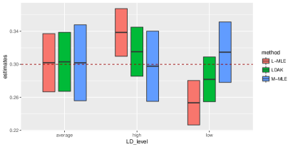
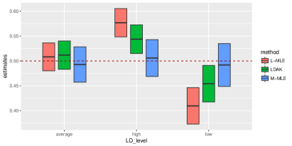
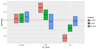
Figure 1: 95% confidence intervals of Euclidean (linear) kernel-based maximum likelihood estimator (L-MLE), MLE with LD adjusted Euclideaen GRM (LDAK), and Mahalanobis kernel-based MLE (M-MLE) with causal variants in different different LD regions, based on 50 independent datasets. For LD-level “average,” $\mathcal{A}=\mathcal{R}_{h}\cup\mathcal{R}_{l}$; “high,” $\mathcal{A}=\mathcal{R}_{h}$; “low,” $\mathcal{A}=\mathcal{R}_{l}$. Underlying $h^{2}$ in the top row are $0.3$ and $0.5$ and marked in red dashed line. $h^{2}$ in the bottom row is 0.7.

In Figure 1, it’s evident that the maximum likelihood estimator with Euclidean kernel is generally biased when causal effects are generated from high or low LD regions. The Euclidean MLE is unbiased when all SNPs are causal (“average” LD-level in Figure 1). In cases where the Euclidean MLE is biased, LDAK has reduced bias, but still some bias remains. The Mahalanobis estimator for $h^{2}$ is unbiased in all of the settings considered here. All three of the methods in Figure 1 are maximum likelihood methods; however, the Mahalanobis MLE has slightly larger standard errors due to the broader distribution of eigenvalues in $\Sigma$, compared to $I$.

In a second set of simulations for estimating total heritability, let $\sigma_{g}^{2}=0.5$, we varied the sparsity along with the location of genetic effects. Given $|\mathcal{A}|$, we let $u_{j}\sim\mathcal{N}(0,\psi_{j})$ for $j\in\mathcal{A}$ with $|\mathcal{A}|=10,50,200$, and $1,000$ and indices in $\mathcal{A}$ sampled uniformly without replacement from the following regions:

• $\mathcal{A}\subset\mathcal{R}_{h}\cup\mathcal{R}_{l}$;

• $\mathcal{A}\subset\mathcal{R}_{h}$;

• $\mathcal{A}\subset\mathcal{R}_{l}$.

For each of these settigns, we simulated 50 independent datasets with a fixed vector of genetic effects generated from the model (this is the fixed-effects heritability model). For each dataset, we computed three estimates for the heritability coefficient: The Euclidean MLE, Mahalanobis MLE, and LDAK. Results are shown in Figure 2.

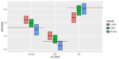
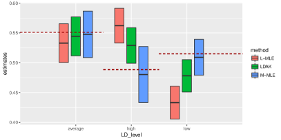
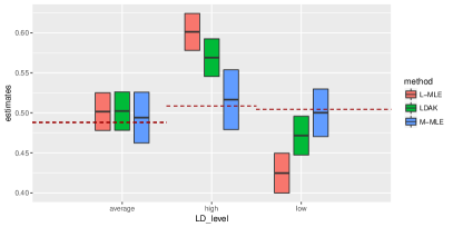
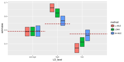
Figure 2: 95% Confidence intervals for the Euclidean kernel maximum likelihood estimator (L-MLE), MLE with LD adjusted Euclidean GRM (LDAK), and Mahalanobis kernel-based MLE (M-MLE) with causal variants from different LD-level regions, based on 50 independent datasets. For LD-level “average,” $\mathcal{A}\subset\mathcal{R}_{h}\cup\mathcal{R}_{l}$; “high,” $\mathcal{A}\subset\mathcal{R}_{h}$; “low,” $\mathcal{A}\subset\mathcal{R}_{l}$. Underlying $h^{2}$ is marked in red dashed line. Sparsity (number of causal SNPs) in the top row is $10$ (L) and $50$ (R); sparsity in the bottom row is $200$ (L) and $1,000$ (R).

In Figure 2, the underlying $h^{2}$ varies across LD levels and simulation settings because it depends on $\Sigma$ and the realization of the random causal loci set $\mathcal{A}$ — recall this is the fixed-effects model. The experiments show that the Euclidean MLE heritability estimator is less stable when effect-sizes become more sparse, which is consistent with results in (Speed et al., 2012). In Figure 2, the Euclidean kernel-based MLE is biased upward when genetic effects are concentrated in high-LD regions, and biased downward when concentrated in low-LD regions. LDAK mitigates the bias of the Euclidean MLE, but does not completely remove it. The Mahalanobis estimator is unbiased in all settings consider in Figure 2.

5.2 Partitioned heritability estimation

In this subsection, we consider partitioned heritability and simulate data from a two variance components linear model (24) with

$$Z\mathbf{u}=Z_{\mathcal{S}}\mathbf{u}_{\mathcal{S}}+Z_{\mathcal{S}^{c}}\mathbf{u}_{\mathcal{S}^{c}}$$

and a causal loci model, where $u_{j}\sim\mathcal{N}(0,\psi_{j})$ and

$$\psi_{j}=\left\{\begin{array}[]{ll}\frac{1}{c_{\mathcal{S}}}\sigma^{2}_{\mathcal{S}}(p_{j}(1-p_{j}))^{-1},&\mbox{if }i\in\mathcal{A}_{1}\subseteq\mathcal{S},\\ \frac{1}{c_{\mathcal{S}^{c}}}\sigma^{2}_{\mathcal{S}^{c}}(p_{j}(1-p_{j}))^{-1},&\mbox{if }i\in\mathcal{A}_{2}\subseteq\mathcal{S}^{c},\\ 0,&\mbox{otherwise}.\end{array}\right.$$

In the first experiment, we let $\mathcal{A}_{1}=\mathcal{S}=\{i\in[m];1\equiv i\ \ (\hbox{mod}4)\}$ and $\mathcal{A}_{2}=\mathcal{S}^{c}$. We would like to estimate $h^{2}_{\mathcal{S}}$, the heritability associated with $\mathcal{S}$, while varying $\sigma^{2}_{\mathcal{S}}=0.1,0.3,0.5$ and keeping $\sigma^{2}_{e}=\sigma^{2}_{\mathcal{S}}+\sigma_{\mathcal{S}^{c}}^{2}=0.5$.

For each setting, we simulated 50 independent datasets, and for each dataset we compute the Mahalanobis partitioned heritability estimator and the restricted maximum likelihood (REML) with linear kernel (Gilmour, Thompson and Cullis, 1995; Yang et al., 2011a). REML finds the maximum likelihood estimator for the two variance components linear model. Summary statistics from these simulations are reported in Figure 3.

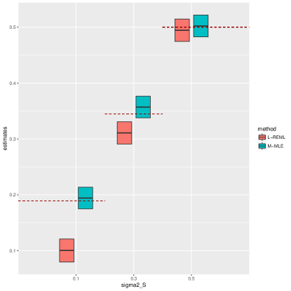
Figure 3: 95% confidence intervals for partitioned heritability estimation with linear REML (L-REML) and Mahalanobis kernel-based MLE (M-MLE), based on 50 independent datasets. Signal strength $\sigma^{2}_{\mathcal{S}}=0.1,0.3,0.5$ of genetic effects indicated on horizontal axis. Underlying $h^{2}_{\mathcal{S}}$ is marked in red dashed line.

The Mahalanobis MLE is an unbiased estimator for the partitioned heritability $h^{2}_{\mathcal{S}}$ in all settings consider in Figure 3. The linear REML estimator underestimates $h^{2}_{\mathcal{S}}$ when $\sigma^{2}_{\mathcal{S}}<0.5$. On the other hand, it’s evident that the linear kernel-based MLE is an unbiased estimator for the variance component $\sigma^{2}_{\mathcal{S}}$. In this example, the discrepancy between the REML and Mahalanobis estimators is due to the difference in estimands for the two methods: Under the definition of partitioned heritability in Section 4.3, $h^{2}_{\mathcal{S}}\neq\sigma_{\mathcal{S}}^{2}$ in general. We’ve argued above that the partitioned heritability coefficient $h^{2}_{\mathcal{S}}$ correctly accounts for causal loci models and LD.

In the next experiment, we set

• $\mathcal{S}=\{m/4+1,\dots,3m/4\}$,

• $\mathcal{A}_{1}=\{m/4+1,m/2\}$,

• $\sigma^{2}_{\mathcal{S}}=0.25$ and $\sigma^{2}_{e}=0.5$.

Let $\mathcal{R}_{l}=\{1,\dots,m/4\}$ and $\mathcal{R}_{h}=\{3m/4+1,\dots,m\}$ be the set of indices corresponding to low and high LD regions in $\mathcal{S}^{c}$, respectively. In this experiment we varied the location of $\mathcal{A}_{2}$, so that

• $\mathcal{A}_{2}=\mathcal{R}_{l}\cup\mathcal{R}_{h}$;

• $\mathcal{A}_{2}=\mathcal{R}_{h}$;

• $\mathcal{A}_{2}=\mathcal{R}_{l}$.

For each simulation setting, we generated 50 random-effects vectors and independent datasets; for each dataset we computed the Mahalanobis estimator and the REML estimator with linear kernel for the partitioned heritability due to $\mathcal{S}$. Summary statistics are reported in Figure 4.

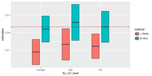
Figure 4: 95% confidence intervals for partitioned heritability estimation with linear REML (L-REML) and Mahalanobis kernel-based MLE (M-MLE), based on 50 independent datasets. Underlying $h^{2}_{\mathcal{S}}$ is marked in red dashed line. Causal loci $\mathcal{S}$ are locat in low-LD region, while causal loci in $\mathcal{S}^{c}$ varies are from regions with varying LD.

In all three settings depicted in Figure 4, the Mahalanobis estimator is an unbiased estimator for

$$h^{2}_{\mathcal{S}}=\frac{\sigma^{2}_{\mathcal{S}}}{\sigma^{2}_{\mathcal{S}}+\sigma^{2}_{\mathcal{S}^{c}}+\sigma^{2}_{e}}=0.25,$$

while the linear REML estimator has downward bias. Note that under this causal loci model, the linear REML estimators are also biased for estimating the variance components; see Table 2. This is due to model misspecifiction – REML assumes that all genetic effects in $\mathcal{S}$ and $\mathcal{S}^{c}$ are iid, but in this causal loci model half of the genetic effects in $\mathcal{S}$ equal 0, i.e. $u_{j}=0$ for $j\in\mathcal{S}\setminus\mathcal{A}_{1}$.

Table 2: Estimated mean (95% confidence interval) of $\sigma^{2}_{\mathcal{S}}$, $\sigma^{2}_{\mathcal{S}^{c}}$ and $\sigma^{2}_{e}$ by linear REML. Based on results from 50 independent datasets.

	Average LD Level		High LD Level		Low LD Level
$\sigma^{2}_{\mathcal{S}}=0.25$	Mean:	0.206	Mean:	0.219	Mean:	0.218
	95%CI:	(0.184,0.228)	95%CI:	(0.192,0.247)	95%CI:	(0.194,0.240)
$\sigma^{2}_{\mathcal{S}^{c}}=0.25$	Mean:	0.235	Mean:	0.292	Mean:	0.199
	95%CI:	(0.210,0.260)	95%CI:	(0.274,0.309)	95%CI:	(0.175,0.223)
$\sigma^{2}_{e}=0.5$	Mean:	0.554	Mean:	0.486	Mean:	0.579
	95%CI:	(0.526,0.582)	95%CI:	(0.457,0.516)	95%CI:	(0.554,0.604)

6 Discussion

In this paper, we studied the Mahalanobis distanced-based GRM for estimating heritability with GWAS data. Under the Mahalanobis kernel, the fixed- and random-effects model are equivalent, which resolves many LD-related inconsistencies in total and partitioned heritability estimation at the modeling level. This paper also re-emphasizes the importance of understanding the underlying LD structure as the LD matrix is required for computing the Mahalanobis distance. An interesting research direction is to study semi-supervised learning methods for estimating the LD structure from unlabeled genotype data (with no corresponding phenotypes) and using this to improve heritability estimation for a specific phenotype of interest; this has connections with recent theoretical work in statistics on the conditionality principle in high dimensions (Azriel, 2018).

Theoretically, the connection between fixed- and random-effects models with the Mahalanobis kernel is most clearly delineated assuming multivariate Gaussian genotypes. However, the simulation results suggest that the proposed estimator performs reliably for genetic data with non-Gaussian genotypes. In this paper, only quantitative traits are considered. An interesting research direction is extending the Mahalanobis MLE results to binary traits in heritability estimation through either the liability or generalized linear model.

Appendix

Proof of Proposition 1.

Without loss of generality, assume that $\mathrm{Var}(y)=1$ and $\mathcal{S}=\{1,\dots,|\mathcal{S}|\}$. Let $\mathbf{u}=(\mathbf{u}_{\mathcal{S}}^{\top},\mathbf{u}_{\mathcal{S}^{c}}^{\top})^{\top}\in\mathcal{R}^{p}$ and $\Sigma=\begin{pmatrix}\Sigma_{\mathcal{S}}&\Sigma_{\mathcal{S},\mathcal{S}^{c}}\\ \Sigma_{\mathcal{S},\mathcal{S}^{c}}^{\top}&\Sigma_{\mathcal{S}^{c}}.\end{pmatrix}$. Then the quadratic form based heritability $h^{2}_{\mathcal{S}}(\mathbf{u},\Sigma)=\mathbf{u}^{\top}\Gamma\mathbf{u}$ where $\Gamma=\begin{pmatrix}\Gamma_{\mathcal{S}}&\Gamma_{\mathcal{S},\mathcal{S}^{c}}\\ \Gamma_{\mathcal{S},\mathcal{S}^{c}}^{\top}&\Gamma_{\mathcal{S}^{c}}\end{pmatrix}$ is a $p\times p$ matrix. Moreover, due to property (i), $0\leq\Gamma\leq\Sigma$. If $\mathbf{u}_{\mathcal{S}}^{c}=0$, $\forall\ \mathbf{u}_{\mathcal{S}}\in\mathcal{R}^{|\mathcal{S}|}$,

$$h^{2} = \mathbf{u}_{\mathcal{S}}^{\top}\Sigma_{\mathcal{S}}\mathbf{u}_{\mathcal{S}},$$

$$h^{2}_{\mathcal{S}} = \mathbf{u}_{\mathcal{S}}^{\top}\Gamma_{\mathcal{S}}\mathbf{u}_{\mathcal{S}}.$$

By property (ii), this implies $\Gamma_{\mathcal{S}}=\Sigma_{\mathcal{S}}$. If $\mathbf{u}_{\mathcal{S}}=0$ and $\mathbf{u}_{\mathcal{S}^{c}}\neq 0$,

$$h^{2} = \mathbf{u}_{\mathcal{S}^{c}}^{\top}\Sigma_{\mathcal{S}^{c}}\mathbf{u}_{\mathcal{S}^{c}},$$

$$h^{2}_{\mathcal{S}} = \mathbf{u}_{\mathcal{S}^{c}}^{\top}\Gamma_{\mathcal{S}^{c}}\mathbf{u}_{\mathcal{S}^{c}}.$$

Then by Property (i) and (ii), $\Gamma_{\mathcal{S}^{c}}<\Sigma_{\mathcal{S}^{c}}$. Next, Property (i) suggests that

$$\Sigma-\Gamma=\begin{pmatrix}0&\Sigma_{\mathcal{S},\mathcal{S}^{c}}-\Gamma_{\mathcal{S},\mathcal{S}^{c}}\\ (\Sigma_{\mathcal{S},\mathcal{S}^{c}}-\Gamma_{\mathcal{S},\mathcal{S}^{c}})^{\top}&\Sigma_{\mathcal{S}^{c}}-\Gamma_{\mathcal{S}^{c}}\end{pmatrix}\geq 0$$

Since $\Sigma_{\mathcal{S}^{c}}-\Gamma_{\mathcal{S}^{c}}>0$, $\Sigma-\Gamma\geq 0$ is equivalent to

$$0-(\Sigma_{\mathcal{S},\mathcal{S}^{c}}-\Gamma_{\mathcal{S},\mathcal{S}^{c}})(\Sigma_{\mathcal{S}^{c}}-\Gamma_{\mathcal{S}^{c}})^{-1}(\Sigma_{\mathcal{S},\mathcal{S}^{c}}-\Gamma_{\mathcal{S},\mathcal{S}^{c}})^{\top} \geq 0$$

$$(\Sigma_{\mathcal{S},\mathcal{S}^{c}}-\Gamma_{\mathcal{S},\mathcal{S}^{c}})(\Sigma_{\mathcal{S}^{c}}-\Gamma_{\mathcal{S}^{c}})^{-1}(\Sigma_{\mathcal{S},\mathcal{S}^{c}}-\Gamma_{\mathcal{S},\mathcal{S}^{c}})^{\top} \leq 0$$

However, $(\Sigma_{\mathcal{S},\mathcal{S}^{c}}-\Gamma_{\mathcal{S},\mathcal{S}^{c}})(\Sigma_{\mathcal{S}^{c}}-\Gamma_{\mathcal{S}^{c}})^{-1}(\Sigma_{\mathcal{S},\mathcal{S}^{c}}-\Gamma_{\mathcal{S},\mathcal{S}^{c}})^{\top}\geq 0$ because $\Sigma-\Gamma\geq 0$ and $\Sigma_{\mathcal{S}^{c}}-\Gamma_{\mathcal{S}^{c}}>0$. Therefore,

$$(\Sigma_{\mathcal{S},\mathcal{S}^{c}}-\Gamma_{\mathcal{S},\mathcal{S}^{c}})(\Sigma_{\mathcal{S}^{c}}-\Gamma_{\mathcal{S}^{c}})^{-1}(\Sigma_{\mathcal{S},\mathcal{S}^{c}}-\Gamma_{\mathcal{S},\mathcal{S}^{c}})^{\top} = 0$$

Thus, $\Gamma_{\mathcal{S},\mathcal{S}^{c}}=\Sigma_{\mathcal{S},\mathcal{S}^{c}}$. Moreover, $\Gamma\geq 0$ implies

$$\Gamma_{\mathcal{S}^{c}}-\Sigma_{\mathcal{S},\mathcal{S}^{c}}^{\top}\Sigma_{\mathcal{S}}^{-1}\Sigma_{\mathcal{S},\mathcal{S}^{c}}\geq 0$$ (26)

We then let

$$\Gamma_{\mathcal{S}^{c}}=\Sigma_{\mathcal{S},\mathcal{S}^{c}}^{\top}\Sigma_{\mathcal{S}}^{-1}\Sigma_{\mathcal{S},\mathcal{S}^{c}}+M,\quad M\geq 0$$

Finally, we would like to prove $M=0$ by contradiction. Suppose that there exist some $\mathbf{u}_{\mathcal{S}^{c}}=\boldsymbol{\beta}$ and $\Sigma$ such that $\boldsymbol{\beta}^{\top}M\tilde{\boldsymbol{\beta}}>0$. Let $\mathbf{u}=(0,\dots,0,\ \boldsymbol{\beta})^{\top}$, then

$$h^{2}_{\mathcal{S}}=\boldsymbol{\beta}^{\top}\Sigma_{\mathcal{S},\mathcal{S}^{c}}^{\top}\Sigma_{\mathcal{S}}^{-1}\Sigma_{\mathcal{S},\mathcal{S}^{c}}\boldsymbol{\beta}+\boldsymbol{\beta}^{\top}M\boldsymbol{\beta}$$

Now let

$$\tilde{\Sigma}=\begin{pmatrix}\Sigma_{\mathcal{S}}&\Sigma_{\mathcal{S},\mathcal{S}^{c}}\\ \Sigma_{\mathcal{S},\mathcal{S}^{c}}^{\top}&\Sigma_{\mathcal{S},\mathcal{S}^{c}}^{\top}\Sigma_{\mathcal{S}}^{-1}\Sigma_{\mathcal{S},\mathcal{S}^{c}}+\dfrac{1}{2}M+\dfrac{\boldsymbol{\beta}^{\top}M\boldsymbol{\beta}}{4\|\boldsymbol{\beta}\|_{2}^{2}}I\end{pmatrix}>0$$

By property (iii), $h^{2}_{\mathcal{S}}(\mathbf{u},\tilde{\Sigma})=h^{2}_{\mathcal{S}}(\mathbf{u},\Sigma)$. However,

$$h^{2}(\mathbf{u},\tilde{\Sigma}) = \boldsymbol{\beta}^{\top}\Sigma_{\mathcal{S},\mathcal{S}^{c}}^{\top}\Sigma_{\mathcal{S}}^{-1}\Sigma_{\mathcal{S},\mathcal{S}^{c}}\boldsymbol{\beta}+\frac{3}{4}\boldsymbol{\beta}^{\top}M\boldsymbol{\beta}$$

$$= h^{2}_{\mathcal{S}}(\mathbf{u},\tilde{\Sigma})-\frac{1}{4}{\boldsymbol{\beta}}^{\top}M\boldsymbol{\beta}$$

This contradicts with Property (i). Therefore, $M=0$ and $\Gamma_{\mathcal{S}^{c}}=\Sigma_{\mathcal{S},\mathcal{S}^{c}}^{\top}\Sigma_{\mathcal{S}}^{-1}\Sigma_{\mathcal{S},\mathcal{S}^{c}}$.

$\Box$

Proof of Proposition 2.

The consistency part of Proposition 2 follows immediately from Theorem 1 of (Dicker and Erdogdu, 2016b). By Theorem 2 of (Dicker and Erdogdu, 2016b),

$$\sqrt{n}(\hat{\eta}^{2}_{C}-\eta^{2}_{C})\overset{\mathcal{D}}{\longrightarrow}\mathcal{N}(0,\psi).$$

where $\psi=(\iota_{2}-\iota_{3}^{2}/\iota_{4})^{-1}$ and

$$\iota_{\alpha}=\frac{1}{2n\sigma_{C^{\perp}}^{2(4-\alpha)}}\mathrm{tr}\left\{\left(\frac{1}{k}W_{C}W_{C}^{\top}\right)^{\alpha-2}\left(\frac{\eta^{2}_{C}}{k}W_{C}W_{C}^{\top}+I\right)^{2-\alpha}\right\}.$$

Let $\mathcal{I}=\frac{1}{k}W_{C}W_{C}^{\top}$ and $\mathcal{J}=\frac{\eta^{2}_{C}}{k}W_{C}W_{C}^{\top}+I$, It follows that

$$\psi=2\sigma^{4}_{C^{\perp}}\left(1-\frac{\mathrm{tr}(\mathcal{I}\mathcal{J}^{-1})^{2}}{n\mathrm{tr}(\mathcal{I}^{2}\mathcal{J}^{-2})}\right)^{-1}.$$

By the Delta method,

$$\sqrt{n}(\hat{h}^{2}_{C}-h^{2})\overset{\mathcal{D}}{\longrightarrow}\mathcal{N}\left(0,\frac{\psi}{(1+\eta^{2}_{C})^{4}}\right).$$

$\Box$

References

- Akdemir and Jannink (2015) {barticle}[author] \bauthor\bsnmAkdemir, \bfnmDeniz\binitsD. and \bauthor\bsnmJannink, \bfnmJean-Luc\binitsJ.-L. (\byear2015). \btitleLocally epistatic genomic relationship matrices for genomic association and prediction. \bjournalGenetics \bvolume199 \bpages857–871. \endbibitem
- Azriel (2018) {barticle}[author] \bauthor\bsnmAzriel, \bfnmDavid\binitsD. (\byear2018). \btitleThe conditionality principle in high-dimensional regression. \bjournalarXiv preprint arXiv:1806.10008. \endbibitem
- Bai et al. (2007) {barticle}[author] \bauthor\bsnmBai, \bfnmZD\binitsZ., \bauthor\bsnmMiao, \bfnmBQ\binitsB., \bauthor\bsnmPan, \bfnmGM\binitsG. \betalet al. (\byear2007). \btitleOn asymptotics of eigenvectors of large sample covariance matrix. \bjournalThe Annals of Probability \bvolume35 \bpages1532–1572. \endbibitem
- Barbiero and Ferrari (2017) {barticle}[author] \bauthor\bsnmBarbiero, \bfnmAlessandro\binitsA. and \bauthor\bsnmFerrari, \bfnmPier Alda\binitsP. A. (\byear2017). \btitleAn R package for the simulation of correlated discrete variables. \bjournalCommunications in Statistics-Simulation and Computation \bvolume46 \bpages5123–5140. \endbibitem
- Barrett et al. (2009) {barticle}[author] \bauthor\bsnmBarrett, \bfnmJeffrey C\binitsJ. C., \bauthor\bsnmClayton, \bfnmDavid G\binitsD. G., \bauthor\bsnmConcannon, \bfnmPatrick\binitsP., \bauthor\bsnmAkolkar, \bfnmBeena\binitsB., \bauthor\bsnmCooper, \bfnmJason D\binitsJ. D., \bauthor\bsnmErlich, \bfnmHenry A\binitsH. A., \bauthor\bsnmJulier, \bfnmCécile\binitsC., \bauthor\bsnmMorahan, \bfnmGrant\binitsG., \bauthor\bsnmNerup, \bfnmJørn\binitsJ., \bauthor\bsnmNierras, \bfnmConcepcion\binitsC. \betalet al. (\byear2009). \btitleGenome-wide association study and meta-analysis find that over 40 loci affect risk of type 1 diabetes. \bjournalNature genetics \bvolume41 \bpages703. \endbibitem
- Bonnet et al. (2015) {barticle}[author] \bauthor\bsnmBonnet, \bfnmAnna\binitsA., \bauthor\bsnmGassiat, \bfnmElisabeth\binitsE., \bauthor\bsnmLévy-Leduc, \bfnmCéline\binitsC. \betalet al. (\byear2015). \btitleHeritability estimation in high dimensional sparse linear mixed models. \bjournalElectronic Journal of Statistics \bvolume9 \bpages2099–2129. \endbibitem
- Bulik-Sullivan et al. (2015) {barticle}[author] \bauthor\bsnmBulik-Sullivan, \bfnmBrendan K\binitsB. K., \bauthor\bsnmLoh, \bfnmPo-Ru\binitsP.-R., \bauthor\bsnmFinucane, \bfnmHilary K\binitsH. K., \bauthor\bsnmRipke, \bfnmStephan\binitsS., \bauthor\bsnmYang, \bfnmJian\binitsJ., \bauthor\bsnmPatterson, \bfnmNick\binitsN., \bauthor\bsnmDaly, \bfnmMark J\binitsM. J., \bauthor\bsnmPrice, \bfnmAlkes L\binitsA. L., \bauthor\bsnmNeale, \bfnmBenjamin M\binitsB. M., \bauthor\bparticleof the \bsnmPsychiatric Genomics Consortium, \bfnmSchizophrenia Working Group\binitsS. W. G. \betalet al. (\byear2015). \btitleLD Score regression distinguishes confounding from polygenicity in genome-wide association studies. \bjournalNature genetics \bvolume47 \bpages291–295. \endbibitem
- International HapMap 3 Consortium and others (2010) {barticle}[author] \bauthor\bsnmInternational HapMap 3 Consortium and others (\byear2010). \btitleIntegrating common and rare genetic variation in diverse human populations. \bjournalNature \bvolume467 \bpages52. \endbibitem
- Davis et al. (2013) {barticle}[author] \bauthor\bsnmDavis, \bfnmLea K\binitsL. K., \bauthor\bsnmYu, \bfnmDongmei\binitsD., \bauthor\bsnmKeenan, \bfnmClare L\binitsC. L., \bauthor\bsnmGamazon, \bfnmEric R\binitsE. R., \bauthor\bsnmKonkashbaev, \bfnmAnuar I\binitsA. I., \bauthor\bsnmDerks, \bfnmEske M\binitsE. M., \bauthor\bsnmNeale, \bfnmBenjamin M\binitsB. M., \bauthor\bsnmYang, \bfnmJian\binitsJ., \bauthor\bsnmLee, \bfnmS Hong\binitsS. H., \bauthor\bsnmEvans, \bfnmPatrick\binitsP. \betalet al. (\byear2013). \btitlePartitioning the heritability of Tourette syndrome and obsessive compulsive disorder reveals differences in genetic architecture. \bjournalPLoS Genet \bvolume9 \bpagese1003864. \endbibitem
- De Maesschalck, Jouan-Rimbaud and Massart (2000) {barticle}[author] \bauthor\bsnmDe Maesschalck, \bfnmRoy\binitsR., \bauthor\bsnmJouan-Rimbaud, \bfnmDelphine\binitsD. and \bauthor\bsnmMassart, \bfnmDésiré L\binitsD. L. (\byear2000). \btitleThe mahalanobis distance. \bjournalChemometrics and intelligent laboratory systems \bvolume50 \bpages1–18. \endbibitem
- Dicker (2014) {barticle}[author] \bauthor\bsnmDicker, \bfnmLee H\binitsL. H. (\byear2014). \btitleVariance estimation in high-dimensional linear models. \bjournalBiometrika \bvolume101 \bpages269–284. \endbibitem
- Dicker and Erdogdu (2016a) {barticle}[author] \bauthor\bsnmDicker, \bfnmLee H\binitsL. H. and \bauthor\bsnmErdogdu, \bfnmMurat A\binitsM. A. (\byear2016a). \btitleFlexible results for quadratic forms with applications to variance components estimation. \bjournalAnn. Stat. \bnoteto appear. \endbibitem
- Dicker and Erdogdu (2016b) {binproceedings}[author] \bauthor\bsnmDicker, \bfnmLee H\binitsL. H. and \bauthor\bsnmErdogdu, \bfnmMurat A\binitsM. A. (\byear2016b). \btitleMaximum likelihood for variance estimation in high-dimensional linear models. In \bbooktitleProceedings of the 19th International Conference on Artificial Intelligence and Statistics \bpages159–167. \endbibitem
- Falconer (1960) {bbook}[author] \bauthor\bsnmFalconer, \bfnmDouglas Scott\binitsD. S. (\byear1960). \btitleIntroduction to quantitative genetics. \bpublisherOliver And Boyd; Edinburgh; London. \endbibitem
- Ferrari and Barbiero (2012) {barticle}[author] \bauthor\bsnmFerrari, \bfnmPier Alda\binitsP. A. and \bauthor\bsnmBarbiero, \bfnmAlessandro\binitsA. (\byear2012). \btitleSimulating ordinal data. \bjournalMultivariate Behavioral Research \bvolume47 \bpages566–589. \endbibitem
- Finucane et al. (2015) {barticle}[author] \bauthor\bsnmFinucane, \bfnmHilary K\binitsH. K., \bauthor\bsnmBulik-Sullivan, \bfnmBrendan\binitsB., \bauthor\bsnmGusev, \bfnmAlexander\binitsA., \bauthor\bsnmTrynka, \bfnmGosia\binitsG., \bauthor\bsnmReshef, \bfnmYakir\binitsY., \bauthor\bsnmLoh, \bfnmPo-Ru\binitsP.-R., \bauthor\bsnmAnttila, \bfnmVerneri\binitsV., \bauthor\bsnmXu, \bfnmHan\binitsH., \bauthor\bsnmZang, \bfnmChongzhi\binitsC., \bauthor\bsnmFarh, \bfnmKyle\binitsK. \betalet al. (\byear2015). \btitlePartitioning heritability by functional annotation using genome-wide association summary statistics. \bjournalNature genetics \bvolume47 \bpages1228–1235. \endbibitem
- Gazal et al. (2017) {barticle}[author] \bauthor\bsnmGazal, \bfnmSteven\binitsS., \bauthor\bsnmFinucane, \bfnmHilary K\binitsH. K., \bauthor\bsnmFurlotte, \bfnmNicholas A\binitsN. A., \bauthor\bsnmLoh, \bfnmPo-Ru\binitsP.-R., \bauthor\bsnmPalamara, \bfnmPier Francesco\binitsP. F., \bauthor\bsnmLiu, \bfnmXuanyao\binitsX., \bauthor\bsnmSchoech, \bfnmArmin\binitsA., \bauthor\bsnmBulik-Sullivan, \bfnmBrendan\binitsB., \bauthor\bsnmNeale, \bfnmBenjamin M\binitsB. M., \bauthor\bsnmGusev, \bfnmAlexander\binitsA. \betalet al. (\byear2017). \btitleLinkage disequilibrium–dependent architecture of human complex traits shows action of negative selection. \bjournalNature genetics \bvolume49 \bpages1421. \endbibitem
- Gibson (2012) {barticle}[author] \bauthor\bsnmGibson, \bfnmGreg\binitsG. (\byear2012). \btitleRare and common variants: twenty arguments. \bjournalNature Reviews Genetics \bvolume13 \bpages135. \endbibitem
- Gilmour, Thompson and Cullis (1995) {barticle}[author] \bauthor\bsnmGilmour, \bfnmArthur R\binitsA. R., \bauthor\bsnmThompson, \bfnmRobin\binitsR. and \bauthor\bsnmCullis, \bfnmBrian R\binitsB. R. (\byear1995). \btitleAverage information REML: an efficient algorithm for variance parameter estimation in linear mixed models. \bjournalBiometrics \bpages1440–1450. \endbibitem
- Golan, Lander and Rosset (2014) {barticle}[author] \bauthor\bsnmGolan, \bfnmDavid\binitsD., \bauthor\bsnmLander, \bfnmEric S\binitsE. S. and \bauthor\bsnmRosset, \bfnmSaharon\binitsS. (\byear2014). \btitleMeasuring missing heritability: inferring the contribution of common variants. \bjournalProceedings of the National Academy of Sciences \bvolume111 \bpagesE5272–E5281. \endbibitem
- Gusev et al. (2013) {barticle}[author] \bauthor\bsnmGusev, \bfnmAlexander\binitsA., \bauthor\bsnmBhatia, \bfnmGaurav\binitsG., \bauthor\bsnmZaitlen, \bfnmNoah\binitsN., \bauthor\bsnmVilhjalmsson, \bfnmBjarni J\binitsB. J., \bauthor\bsnmDiogo, \bfnmDorothée\binitsD., \bauthor\bsnmStahl, \bfnmEli A\binitsE. A., \bauthor\bsnmGregersen, \bfnmPeter K\binitsP. K., \bauthor\bsnmWorthington, \bfnmJane\binitsJ., \bauthor\bsnmKlareskog, \bfnmLars\binitsL., \bauthor\bsnmRaychaudhuri, \bfnmSoumya\binitsS. \betalet al. (\byear2013). \btitleQuantifying missing heritability at known GWAS loci. \bjournalPLoS genetics \bvolume9 \bpagese1003993. \endbibitem
- Gusev et al. (2014) {barticle}[author] \bauthor\bsnmGusev, \bfnmAlexander\binitsA., \bauthor\bsnmLee, \bfnmS Hong\binitsS. H., \bauthor\bsnmTrynka, \bfnmGosia\binitsG., \bauthor\bsnmFinucane, \bfnmHilary\binitsH., \bauthor\bsnmVilhjálmsson, \bfnmBjarni J\binitsB. J., \bauthor\bsnmXu, \bfnmHan\binitsH., \bauthor\bsnmZang, \bfnmChongzhi\binitsC., \bauthor\bsnmRipke, \bfnmStephan\binitsS., \bauthor\bsnmBulik-Sullivan, \bfnmBrendan\binitsB., \bauthor\bsnmStahl, \bfnmEli\binitsE. \betalet al. (\byear2014). \btitlePartitioning heritability of regulatory and cell-type-specific variants across 11 common diseases. \bjournalThe American Journal of Human Genetics \bvolume95 \bpages535–552. \endbibitem
- Haseman and Elston (1972) {barticle}[author] \bauthor\bsnmHaseman, \bfnmJ. K.\binitsJ. K. and \bauthor\bsnmElston, \bfnmR. C.\binitsR. C. (\byear1972). \btitleThe investigation of linkage between a quantitative trait and a marker locus. \bjournalBehav. Genet. \bvolume2 \bpages3–19. \endbibitem
- Hayes, Visscher and Goddard (2009) {barticle}[author] \bauthor\bsnmHayes, \bfnmBen John\binitsB. J., \bauthor\bsnmVisscher, \bfnmPeter M\binitsP. M. and \bauthor\bsnmGoddard, \bfnmMichael E\binitsM. E. (\byear2009). \btitleIncreased accuracy of artificial selection by using the realized relationship matrix. \bjournalGenetics research \bvolume91 \bpages47–60. \endbibitem
- Henderson (1950) {barticle}[author] \bauthor\bsnmHenderson, \bfnmC. R.\binitsC. R. (\byear1950). \btitleAbstract: Estimation of genetic parameters. \bjournalAnn. Math. Stat. \bvolume21 \bpages309–310. \endbibitem
- Henderson (1984) {barticle}[author] \bauthor\bsnmHenderson, \bfnmCR\binitsC. (\byear1984). \btitleApplications of linear models in animal breeding. \endbibitem
- Hindorff et al. (2009) {barticle}[author] \bauthor\bsnmHindorff, \bfnmLucia A\binitsL. A., \bauthor\bsnmSethupathy, \bfnmPraveen\binitsP., \bauthor\bsnmJunkins, \bfnmHeather A\binitsH. A., \bauthor\bsnmRamos, \bfnmErin M\binitsE. M., \bauthor\bsnmMehta, \bfnmJayashri P\binitsJ. P., \bauthor\bsnmCollins, \bfnmFrancis S\binitsF. S. and \bauthor\bsnmManolio, \bfnmTeri A\binitsT. A. (\byear2009). \btitlePotential etiologic and functional implications of genome-wide association loci for human diseases and traits. \bjournalProceedings of the National Academy of Sciences \bvolume106 \bpages9362–9367. \endbibitem
- Janson, Barber and Candes (2017) {barticle}[author] \bauthor\bsnmJanson, \bfnmLucas\binitsL., \bauthor\bsnmBarber, \bfnmRina Foygel\binitsR. F. and \bauthor\bsnmCandes, \bfnmEmmanuel\binitsE. (\byear2017). \btitleEigenPrism: inference for high dimensional signal-to-noise ratios. \bjournalJournal of the Royal Statistical Society: Series B (Statistical Methodology) \bvolume79 \bpages1037–1065. \endbibitem
- Kang et al. (2010) {barticle}[author] \bauthor\bsnmKang, \bfnmHyun Min\binitsH. M., \bauthor\bsnmSul, \bfnmJae Hoon\binitsJ. H., \bauthor\bsnmZaitlen, \bfnmNoah A\binitsN. A., \bauthor\bsnmKong, \bfnmSit-yee\binitsS.-y., \bauthor\bsnmFreimer, \bfnmNelson B\binitsN. B., \bauthor\bsnmSabatti, \bfnmChiara\binitsC., \bauthor\bsnmEskin, \bfnmEleazar\binitsE. \betalet al. (\byear2010). \btitleVariance component model to account for sample structure in genome-wide association studies. \bjournalNature genetics \bvolume42 \bpages348. \endbibitem
- Kostem and Eskin (2013) {barticle}[author] \bauthor\bsnmKostem, \bfnmEmrah\binitsE. and \bauthor\bsnmEskin, \bfnmEleazar\binitsE. (\byear2013). \btitleImproving the accuracy and efficiency of partitioning heritability into the contributions of genomic regions. \bjournalThe American Journal of Human Genetics \bvolume92 \bpages558–564. \endbibitem
- Lange (2003) {bbook}[author] \bauthor\bsnmLange, \bfnmKenneth\binitsK. (\byear2003). \btitleMathematical and statistical methods for genetic analysis. \bpublisherSpringer Science & Business Media. \endbibitem
- Lee et al. (2013) {barticle}[author] \bauthor\bsnmLee, \bfnmS Hong\binitsS. H., \bauthor\bsnmYang, \bfnmJian\binitsJ., \bauthor\bsnmChen, \bfnmGuo-Bo\binitsG.-B., \bauthor\bsnmRipke, \bfnmStephan\binitsS., \bauthor\bsnmStahl, \bfnmEli A\binitsE. A., \bauthor\bsnmHultman, \bfnmChristina M\binitsC. M., \bauthor\bsnmSklar, \bfnmPamela\binitsP., \bauthor\bsnmVisscher, \bfnmPeter M\binitsP. M., \bauthor\bsnmSullivan, \bfnmPatrick F\binitsP. F., \bauthor\bsnmGoddard, \bfnmMichael E\binitsM. E. \betalet al. (\byear2013). \btitleEstimation of SNP heritability from dense genotype data. \bjournalThe American Journal of Human Genetics \bvolume93 \bpages1151–1155. \endbibitem
- Lee et al. (2016) {barticle}[author] \bauthor\bsnmLee, \bfnmPhil H\binitsP. H., \bauthor\bsnmBaker, \bfnmJustin T\binitsJ. T., \bauthor\bsnmHolmes, \bfnmAvram J\binitsA. J., \bauthor\bsnmJahanshad, \bfnmNeda\binitsN., \bauthor\bsnmGe, \bfnmTian\binitsT., \bauthor\bsnmJung, \bfnmJae-Yoon\binitsJ.-Y., \bauthor\bsnmCruz, \bfnmYanela\binitsY., \bauthor\bsnmManoach, \bfnmDara S\binitsD. S., \bauthor\bsnmHibar, \bfnmDerrek P\binitsD. P., \bauthor\bsnmFaskowitz, \bfnmJoshua\binitsJ. \betalet al. (\byear2016). \btitlePartitioning heritability analysis reveals a shared genetic basis of brain anatomy and schizophrenia. \bjournalMolecular psychiatry \bvolume21 \bpages1680. \endbibitem
- Lynch et al. (1998) {bbook}[author] \bauthor\bsnmLynch, \bfnmMichael\binitsM., \bauthor\bsnmWalsh, \bfnmBruce\binitsB. \betalet al. (\byear1998). \btitleGenetics and analysis of quantitative traits \bvolume1. \bpublisherSinauer Sunderland, MA. \endbibitem
- Mahalanobis (1936) {binproceedings}[author] \bauthor\bsnmMahalanobis, \bfnmPrasanta Chandra\binitsP. C. (\byear1936). \btitleOn the generalized distance in statistics. \bpublisherNational Institute of Science of India. \endbibitem
- Majumdar, Witte and Ghosh (2015) {barticle}[author] \bauthor\bsnmMajumdar, \bfnmArunabha\binitsA., \bauthor\bsnmWitte, \bfnmJohn S\binitsJ. S. and \bauthor\bsnmGhosh, \bfnmSaurabh\binitsS. (\byear2015). \btitleSemiparametric allelic tests for mapping multiple phenotypes: binomial regression and Mahalanobis distance. \bjournalGenetic epidemiology \bvolume39 \bpages635–650. \endbibitem
- Mathew, Léon and Sillanpää (2018) {barticle}[author] \bauthor\bsnmMathew, \bfnmBoby\binitsB., \bauthor\bsnmLéon, \bfnmJens\binitsJ. and \bauthor\bsnmSillanpää, \bfnmMikko J\binitsM. J. (\byear2018). \btitleA novel linkage-disequilibrium corrected genomic relationship matrix for SNP-heritability estimation and genomic prediction. \bjournalHeredity \bvolume120 \bpages356. \endbibitem
- Meuwissen and Goddard (2001) {barticle}[author] \bauthor\bsnmMeuwissen, \bfnmHayes BJ\binitsH. B. \bsuffixT. H. E. and \bauthor\bsnmGoddard, \bfnmME\binitsM. (\byear2001). \btitlePrediction of total genetic value using genome-wide dense marker maps. \bjournalGenetics \bvolume157 \bpages1819–1829. \endbibitem
- Patterson, Price and Reich (2006) {barticle}[author] \bauthor\bsnmPatterson, \bfnmNick\binitsN., \bauthor\bsnmPrice, \bfnmAlkes L\binitsA. L. and \bauthor\bsnmReich, \bfnmDavid\binitsD. (\byear2006). \btitlePopulation structure and eigenanalysis. \bjournalPLoS genetics \bvolume2 \bpagese190. \endbibitem
- Powell, Visscher and Goddard (2010) {barticle}[author] \bauthor\bsnmPowell, \bfnmJoseph E\binitsJ. E., \bauthor\bsnmVisscher, \bfnmPeter M\binitsP. M. and \bauthor\bsnmGoddard, \bfnmMichael E\binitsM. E. (\byear2010). \btitleReconciling the analysis of IBD and IBS in complex trait studies. \bjournalNature Reviews Genetics \bvolume11 \bpages800. \endbibitem
- Price et al. (2010) {barticle}[author] \bauthor\bsnmPrice, \bfnmAlkes L\binitsA. L., \bauthor\bsnmZaitlen, \bfnmNoah A\binitsN. A., \bauthor\bsnmReich, \bfnmDavid\binitsD. and \bauthor\bsnmPatterson, \bfnmNick\binitsN. (\byear2010). \btitleNew approaches to population stratification in genome-wide association studies. \bjournalNature Reviews Genetics \bvolume11 \bpages459–463. \endbibitem
- Pritchard (2001) {barticle}[author] \bauthor\bsnmPritchard, \bfnmJonathan K\binitsJ. K. (\byear2001). \btitleAre rare variants responsible for susceptibility to complex diseases? \bjournalThe American Journal of Human Genetics \bvolume69 \bpages124–137. \endbibitem
- Purcell et al. (2007) {barticle}[author] \bauthor\bsnmPurcell, \bfnmShaun\binitsS., \bauthor\bsnmNeale, \bfnmBenjamin\binitsB., \bauthor\bsnmTodd-Brown, \bfnmKathe\binitsK., \bauthor\bsnmThomas, \bfnmLori\binitsL., \bauthor\bsnmFerreira, \bfnmManuel AR\binitsM. A., \bauthor\bsnmBender, \bfnmDavid\binitsD., \bauthor\bsnmMaller, \bfnmJulian\binitsJ., \bauthor\bsnmSklar, \bfnmPamela\binitsP., \bauthor\bsnmDe Bakker, \bfnmPaul IW\binitsP. I., \bauthor\bsnmDaly, \bfnmMark J\binitsM. J. \betalet al. (\byear2007). \btitlePLINK: a tool set for whole-genome association and population-based linkage analyses. \bjournalThe American Journal of Human Genetics \bvolume81 \bpages559–575. \endbibitem
- Schoech et al. (2017) {barticle}[author] \bauthor\bsnmSchoech, \bfnmArmin\binitsA., \bauthor\bsnmJordan, \bfnmDaniel\binitsD., \bauthor\bsnmLoh, \bfnmPo-Ru\binitsP.-R., \bauthor\bsnmGazal, \bfnmSteven\binitsS., \bauthor\bsnmO’Connor, \bfnmLuke\binitsL., \bauthor\bsnmBalick, \bfnmDaniel J\binitsD. J., \bauthor\bsnmPalamara, \bfnmPier F\binitsP. F., \bauthor\bsnmFinucane, \bfnmHilary\binitsH., \bauthor\bsnmSunyaev, \bfnmShamil R\binitsS. R. and \bauthor\bsnmPrice, \bfnmAlkes L\binitsA. L. (\byear2017). \btitleQuantification of frequency-dependent genetic architectures and action of negative selection in 25 UK Biobank traits. \bjournalbioRxiv \bpages188086. \endbibitem
- Schwartzman et al. (2017) {barticle}[author] \bauthor\bsnmSchwartzman, \bfnmArmin\binitsA., \bauthor\bsnmSchork, \bfnmAndrew J\binitsA. J., \bauthor\bsnmZablocki, \bfnmRong\binitsR. and \bauthor\bsnmThompson, \bfnmWesley K\binitsW. K. (\byear2017). \btitleA simple, consistent estimator of heritability for genome-wide association studies. \bjournalbioRxiv \bpages204446. \endbibitem
- Speed and Balding (2015) {barticle}[author] \bauthor\bsnmSpeed, \bfnmDoug\binitsD. and \bauthor\bsnmBalding, \bfnmDavid J\binitsD. J. (\byear2015). \btitleRelatedness in the post-genomic era: is it still useful? \bjournalNature Reviews Genetics \bvolume16 \bpages33. \endbibitem
- Speed et al. (2012) {barticle}[author] \bauthor\bsnmSpeed, \bfnmD.\binitsD., \bauthor\bsnmHemani, \bfnmG.\binitsG., \bauthor\bsnmJohnson, \bfnmM. R.\binitsM. R. and \bauthor\bsnmBalding, \bfnmD. J.\binitsD. J. (\byear2012). \btitleImproved heritability estimation from genome-wide SNPs. \bjournalAm. J. Hum. Genet. \bvolume91 \bpages1011–1021. \endbibitem
- Stahl et al. (2010) {barticle}[author] \bauthor\bsnmStahl, \bfnmEli A\binitsE. A., \bauthor\bsnmRaychaudhuri, \bfnmSoumya\binitsS., \bauthor\bsnmRemmers, \bfnmElaine F\binitsE. F., \bauthor\bsnmXie, \bfnmGang\binitsG., \bauthor\bsnmEyre, \bfnmStephen\binitsS., \bauthor\bsnmThomson, \bfnmBrian P\binitsB. P., \bauthor\bsnmLi, \bfnmYonghong\binitsY., \bauthor\bsnmKurreeman, \bfnmFina AS\binitsF. A., \bauthor\bsnmZhernakova, \bfnmAlexandra\binitsA., \bauthor\bsnmHinks, \bfnmAnne\binitsA. \betalet al. (\byear2010). \btitleGenome-wide association study meta-analysis identifies seven new rheumatoid arthritis risk loci. \bjournalNature genetics \bvolume42 \bpages508. \endbibitem
- Stahl et al. (2012) {barticle}[author] \bauthor\bsnmStahl, \bfnmEli A\binitsE. A., \bauthor\bsnmWegmann, \bfnmDaniel\binitsD., \bauthor\bsnmTrynka, \bfnmGosia\binitsG., \bauthor\bsnmGutierrez-Achury, \bfnmJavier\binitsJ., \bauthor\bsnmDo, \bfnmRon\binitsR., \bauthor\bsnmVoight, \bfnmBenjamin F\binitsB. F., \bauthor\bsnmKraft, \bfnmPeter\binitsP., \bauthor\bsnmChen, \bfnmRobert\binitsR., \bauthor\bsnmKallberg, \bfnmHenrik J\binitsH. J., \bauthor\bsnmKurreeman, \bfnmFina AS\binitsF. A. \betalet al. (\byear2012). \btitleBayesian inference analyses of the polygenic architecture of rheumatoid arthritis. \bjournalNature genetics \bvolume44 \bpages483. \endbibitem
- Visscher, Hill and Wray (2008) {barticle}[author] \bauthor\bsnmVisscher, \bfnmPeter M\binitsP. M., \bauthor\bsnmHill, \bfnmWilliam G\binitsW. G. and \bauthor\bsnmWray, \bfnmNaomi R\binitsN. R. (\byear2008). \btitleHeritability in the genomics era—concepts and misconceptions. \bjournalNature reviews genetics \bvolume9 \bpages255. \endbibitem
- Yang et al. (2010) {barticle}[author] \bauthor\bsnmYang, \bfnmJ.\binitsJ., \bauthor\bsnmBenyamin, \bfnmB.\binitsB., \bauthor\bsnmMcEvoy, \bfnmB. P.\binitsB. P., \bauthor\bsnmGordon, \bfnmS.\binitsS., \bauthor\bsnmHenders, \bfnmA. K.\binitsA. K., \bauthor\bsnmNyholt, \bfnmD. R.\binitsD. R., \bauthor\bsnmMadden, \bfnmP. A.\binitsP. A., \bauthor\bsnmHeath, \bfnmA. C.\binitsA. C., \bauthor\bsnmMartin, \bfnmN. G.\binitsN. G., \bauthor\bsnmMontgomery, \bfnmG. W.\binitsG. W., \bauthor\bsnmGoddard, \bfnmM. E.\binitsM. E. and \bauthor\bsnmVisscher, \bfnmP. M.\binitsP. M. (\byear2010). \btitleCommon SNPs explain a large proportion of the heritability for human height. \bjournalNat. Genet. \bvolume42 \bpages565–569. \endbibitem
- Yang et al. (2011a) {barticle}[author] \bauthor\bsnmYang, \bfnmJian\binitsJ., \bauthor\bsnmLee, \bfnmS Hong\binitsS. H., \bauthor\bsnmGoddard, \bfnmMichael E\binitsM. E. and \bauthor\bsnmVisscher, \bfnmPeter M\binitsP. M. (\byear2011a). \btitleGCTA: a tool for genome-wide complex trait analysis. \bjournalThe American Journal of Human Genetics \bvolume88 \bpages76–82. \endbibitem
- Yang et al. (2011b) {barticle}[author] \bauthor\bsnmYang, \bfnmJian\binitsJ., \bauthor\bsnmManolio, \bfnmTeri A\binitsT. A., \bauthor\bsnmPasquale, \bfnmLouis R\binitsL. R., \bauthor\bsnmBoerwinkle, \bfnmEric\binitsE., \bauthor\bsnmCaporaso, \bfnmNeil\binitsN., \bauthor\bsnmCunningham, \bfnmJulie M\binitsJ. M., \bauthor\bsnmDe Andrade, \bfnmMariza\binitsM., \bauthor\bsnmFeenstra, \bfnmBjarke\binitsB., \bauthor\bsnmFeingold, \bfnmEleanor\binitsE., \bauthor\bsnmHayes, \bfnmM Geoffrey\binitsM. G. \betalet al. (\byear2011b). \btitleGenome partitioning of genetic variation for complex traits using common SNPs. \bjournalNature genetics \bvolume43 \bpages519. \endbibitem
- Yang et al. (2015) {barticle}[author] \bauthor\bsnmYang, \bfnmJian\binitsJ., \bauthor\bsnmBakshi, \bfnmAndrew\binitsA., \bauthor\bsnmZhu, \bfnmZhihong\binitsZ., \bauthor\bsnmHemani, \bfnmGibran\binitsG., \bauthor\bsnmVinkhuyzen, \bfnmAnna AE\binitsA. A., \bauthor\bsnmLee, \bfnmSang Hong\binitsS. H., \bauthor\bsnmRobinson, \bfnmMatthew R\binitsM. R., \bauthor\bsnmPerry, \bfnmJohn RB\binitsJ. R., \bauthor\bsnmNolte, \bfnmIlja M\binitsI. M., \bauthor\bparticlevan \bsnmVliet-Ostaptchouk, \bfnmJana V\binitsJ. V. \betalet al. (\byear2015). \btitleGenetic variance estimation with imputed variants finds negligible missing heritability for human height and body mass index. \bjournalNature genetics \bvolume47 \bpages1114. \endbibitem
- Zaitlen and Kraft (2012) {barticle}[author] \bauthor\bsnmZaitlen, \bfnmN. A.\binitsN. A. and \bauthor\bsnmKraft, \bfnmP.\binitsP. (\byear2012). \btitleHeritability in the genome-wide association era. \bjournalHum. Genet. \bvolume131 \bpages1655–1664. \endbibitem
- Zhou et al. (2017) {barticle}[author] \bauthor\bsnmZhou, \bfnmXiang\binitsX. \betalet al. (\byear2017). \btitleA unified framework for variance component estimation with summary statistics in genome-wide association studies. \bjournalThe Annals of Applied Statistics \bvolume11 \bpages2027–2051. \endbibitem