Sentiment Analysis of Czech Texts: An Algorithmic Survey

Abstract

In the area of online communication, commerce and transactions, analyzing sentiment polarity of texts written in various natural languages has become crucial. While there have been a lot of contributions in resources and studies for the English language, “smaller” languages like Czech have not received much attention. In this survey, we explore the effectiveness of many existing machine learning algorithms for sentiment analysis of Czech Facebook posts and product reviews. We report the sets of optimal parameter values for each algorithm and the scores in both datasets. We finally observe that support vector machines are the best classifier and efforts to increase performance even more with bagging, boosting or voting ensemble schemes fail to do so.

1 INTRODUCTION

Sentiment Analysis is considered as the automated analysis of sentiments, emotions or opinions expressed in texts towards certain entities [Medhat et al., 2014]. The proliferation of online commerce and customer feedback has significantly motivated companies to invest in intelligent text analysis tools and technologies where sentiment analysis plays a crucial role. There have traditionally been two main approaches to sentiment analysis. The first one uses unsupervised algorithms, sentiment lexicons and word similarity measures to “mine” emotions in raw texts. The second uses emotionally-labeled text datasets to train supervised (or deep supervised) algorithms and use them to predict emotions in other documents. Naturally, most of sentiment analysis research has been conducted for the English language. Chinese [Zhang et al., 2018, Peng et al., 2017, Wu et al., 2015] and Spanish [Tellez et al., 2017, Miranda and Guzmán, 2017] have also received a considerable extra attention in the last years. “Smaller” languages like Czech have seen fewer efforts in this aspect. It is thus much easier to find online data resources for English than for other languages [Çano Erion and Maurizio, 2015]. One of the first attempts to create sentiment annotated resources of Czech texts dates back in 2012 [Veselovská et al., 2012]. Authors released three datasets of news articles, movie reviews, and product reviews. A subsequent work consisted in creating a Czech dataset of information technology product reviews, their aspects and customers’ attitudes towards those aspects [Tamchyna et al., 2015]. This latter dataset is an essential basis for performing aspect-based sentiment analysis experiments [Tamchyna and Veselovská, 2016]. Another available resource is a dataset of ten thousand Czech Facebook posts and the corresponding emotional labels [Habernal et al., 2013]. The authors report various experimental results with Support Vector Machine (SVM) and Maximum Entropy (ME) classifiers. Despite the creation of the resources mentioned above and the results reported by the corresponding authors, there is still little evidence about the performance of various techniques and algorithms on sentiment analysis of Czech texts. In this paper, we perform an empirical survey, probing many popular supervised learning algorithms on sentiment prediction of Czech Facebook posts and product reviews. We perform document-level analysis considering the text part (that is usually short) as a single document and explore various parameters of Tf-Idf vectorizer and each classification algorithms reporting the optimal ones. According to our results, SVM (Support Vector Machine) is the best player, shortly followed by Logistic Regression (LR) and Naïve Bayes (NB). Moreover, we observe that ensemble techniques like Random Forests (RF), Adaptive Boosting (AdaBoost) or voting schemes do not increase the performance of the basic classifiers. The rest of the paper is structured as follows: Section 2 presents some details and statistics about the two Czech datasets we used. Section 3 describes the text preprocessing steps and vectorizer parameters we grid-searched. Section 4 presents in details the grid-searched parameters and values of all classifiers. In Section 5, we report the optimal parameter values and test scores in each dataset. Finally, Section 6 concludes and presents possible future contributions.

2 DATASETS

Attribute	Mall	Facebook
Records	11K	10K
Tokens	151K	105K
Av. Length	13	10
Classes	2	3
Negative	4356	1991
Neutral	-	5174
Positive	7274	2587

Table 1: Statistics about the two datasets

2.1 Czech Facebook Dataset

Czech Facebook dataset was created by collecting posts from popular Facebook pages in Czech [Habernal et al., 2013]. The ten thousand records were independently revised by two annotators. Two other annotators were involved in cases of disagreement. To estimate inter-annotator agreement, they used Cohen’s kappa coefficient which was about 0.66. Each post was labeled as negative, neutral or positive. There were yet a few samples that revealed both negative and positive sentiments and were marked as bipolar. Same as the authors in their paper, we removed the bipolar category from our experimental set to avoid ambiguity and used the remaining 9752 samples. A few data samples are illustrated in Figure 1.

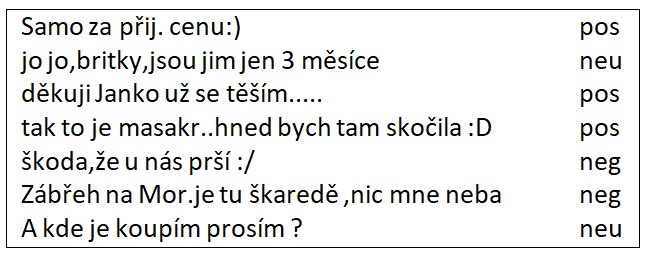
Figure 1: Samples from Czech Facebook dataset

2.2 Mall.cz Reviews Dataset

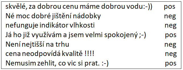
Figure 2: Samples from Mall reviews dataset

The second dataset we use contains user reviews about household devices purchased at mall.cz [Veselovská et al., 2012]. The reviews are evaluative in nature (users apprising items they bought) and were categorized as negative or positive only. Some minor problems they carry are the grammatical or typing errors that frequently appear in their texts [Veselovská, 2017]. In Table 1 we present some rounded statistics about the two datasets. As we can see, Mall product reviews are slightly longer (13 vs. 10 tokens) than Czech Facebook posts. We also see that the number of data samples in each sentiment category are unbalanced in both cases. A few samples of Mall reviews are illustrated in Figure 2.

Vectorizer	Parameters	GS Values
Tf-Idf	ngram range	(1,1),  (1,2),  (1,3)
	stop words	Czech,  None
	smooth idf	True,  False
	norm	l1,  l2,  None

Table 2: Tf-Idf vectorizer grid-searched parameters

3 PREPROCESSING AND VECTORIZATION

Basic preprocessing steps were applied to each text field of the records. First, any remaining markup tags were removed, and everything was lowercased. At this point, we saved all smiley patterns (e.g., “:P”, “:)”, “:(”, “:-(”, “:-)”, “:D”) appearing in each record. Smileys are essential features in sentiment analysis tasks and should not be lost from the further text cleaning steps. Stanford CoreNLP tokenizer was employed for tokenizing. Numbers, punctuation, and special symbols were removed. At this point, we copied back the smiley patterns to each of the text samples. No stemming or lemmatization was applied.

As vectorizer, we chose to experiment with Tf-Idf which has been proved very effective with texts since long time ago [Joachims, 1998, Jing et al., 2002]. Tf-Idf gives the opportunity to work with various n-grams as features (ngram range parameter). We limited our experiments to single words, bigrams, and trigrams only since texts are usually short in both datasets. It is also very common in such experiments to remove a subset of words known as stop words that carry little or no semantic value. In our experiments we tried with full vocabulary or removing Czech stopwords that are defined at https://pypi.org/project/stop-words/ package. Other parameters we explored are smooth idf and norm. The former adds one to document frequencies to smooth Idf weights when computing Tf-Idf score. The latter is used to normalize term vectors (None for no normalization). The parameters and the corresponding grid-searched values of Tf-Idf are listed in Table 2.

Algorithm	Parameters	Grid-Searched Values
SVM	C	0.0001, 0.001, 0.01, 0.1, 1, 10, 100, 1000
	gamma	0.5, 0.1, 0.05, 0.01, 0.005, 0.001, 0.0005, 0.0001
	kernel	linear, rbf, poly, sigmoid
NuSVM	nu	0.35, 0.4, 0.45, 0.5, 0.55, 0.6, 0.65
	kernel	linear, rbf, poly, sigmoid
RF	max depth	None, 10, 20, 30, 40, 50, 60, 70, 80, 90
	max feat	10, 20, 30, 40, 50, sqrt, None
	n est	50, 100, 200, 400, 700, 1000
LR	C	0.0001, 0.001, 0.01, 0.1, 1, 10, 100, 1000
	class weight	balanced, None
	penalty	l1, l2
MLP	alpha	0.0001, 0.0005, 0.001, 0.005, 0.01, 0.05, 0.1, 0.5
	layer sizes	$(10,20,40,60,80,100)\times(1,2,3,4)$
	activation	identity, logistic, tanh, relu
	solver	lbfgs, sgd, adam
NB	alpha	0.0001, 0.0005, 0.001, 0.005, 0.01, 0.05, 0.1, 0.5
	fit prior	True, False
ME	method	gis, iis, megam, tadm

Table 3: Grid-searched parameters and values of each algorithm

Besides using this traditional approach based on Tf-Idf or similar vectorizers, it is also possible to analyze text by means of the more recent dense representations called word embeddings [Mikolov et al., 2013, Pennington et al., 2014]. These embeddings are basically dense vectors (e.g., 300 dimensions each) that are obtained for every vocabulary word of a language when large text collections are fed to neural networks. The advantage of word embeddings over bag-of-word representation and Tf-Idf vectorizer is their lower dimensionality which is essential when working with neural networks. It still takes a lot of text data (e.g., many thousands of samples) to generate high-quality embeddings and achieve reasonable classification performance [Çano and Morisio, 2017]. A neural network architecture for sentiment analysis based on word embeddings is described by [Çano and Morisio, 2018]. We applied that architecture on the two Czech datasets we are using here and observed that there was severe over-fitting, even with dropout regularization. For this reason, in the next section, we report results of simpler supervised algorithms and multilayer perceptron only, omitting experiments with deeper neural networks.

4 SUPERVISED ALGORITHMS

We explored various supervised algorithms that have become popular in recent years and grid-searched their main parameters. Support Vector Machines have been successfully used for solving both classification and regression problems since back in the nineties when they were invented [Boser et al., 1992, Cortes and Vapnik, 1995]. They introduced the notion of hard and soft margins (separation hyperplanes) for optimal separation of class samples. Moreover, the kernel parameter enables them to perform well even with data that are not linearly separable by transforming the feature space [Kocsor and Tóth, 2004]. The C parameter is the error penalty term that tries to balance between a small margin with fewer classification errors and larger margin with more errors. The last parameter we tried is gamma that represents the kernel coefficient for “rfb”, “poly” and “sigmoid” (non linear) kernels. The other algorithm we tried is NuSVM which is very similar to SVM. The only difference is that a new parameter (nu) is utilized to control the number of support vectors. Random Forests (RF) were also invented in the 90s [Ho, 1995, Ho, 1998]. They average results of multiple decision trees (bagging) aiming for lower variance. Among the many parameters, we explored max depth which limits the depth of decision trees. We also grid-searched max feat, the maximal number of features to consider for best tree split. If “sqrt” is given, it will use the square root of total features. If “None” is given then it will use all features. Finally, n est dictates the number of trees (estimators) that will be used. Obviously, more trees may produce better results but they also increase the computation time. Logistic Regression is probably the most basic classifier that still provides reasonably good results for a wide variety of problems. It uses a logistic function to determine the probability of a value belonging to a class or not. C parameter represents the inverse of the regularization term and is important to prevent overfitting. We also explored the class weight parameter which sets weights to sample classes inversely proportional to class frequencies in the input data (for balanced). If None is given, all classes have the same weight. Finally, penalty parameter specifies the norm to use when computing the cost function. To have an idea about the performance of small and shallow neural networks on small datasets, we tried Multilayer Perceptron (MLP) classifier. It comes with a rich set of parameters such as alpha which is the regularization term, solver which is the weight optimization algorithm used during training or activation that is the function used in each neuron of hidden layers to determine its output value. The most critical parameter is layer sizes that specifies the number of neurons in each hidden layer. We tried many tuples such as (10, 1), (20, 1), $\dots$, (100, 4) where the first number is for the neurons and the second for the layer they belong to. Same as Logistic Regression, Naïve Bayes is also a very simple and popular classifier that provides high-quality solutions to many problems. It is based on Bayes theorem:

$$P(A\mid B)=\frac{P(B\mid A)\,P(A)}{P(B)}$$ (1)

which shows a way to get the probability of A given evidence B. For Naïve Bayes, we probed alpha which is the smoothing parameter (dealing with words not in training data) and fit prior for learning (or not) class prior probabilities. The last algorithm we explored is Maximum Entropy classifier. It is a generalization of Naïve Bayes providing the possibility to use a single parameter for associating a feature with more than one label and captures the frequencies of individual joint-features. We explored four of the implementation methods that are available. All algorithms, their parameters, and the grid-searched values are summarized in Table 3.

5 RESULTS

Algorithm	Step	Optimal Parameter Values
SVM	vect	ngram range: (1, 2), smooth idf: False, stop words: None, norm: l2
	clf	C: 100, gamma: 0.005, kernel: rbf
NuSVM	vect	ngram range: (1, 2), smooth idf: True, stop words: None, norm: l2
	clf	kernel: linear, nu: 0.5
RF	vect	ngram range: (1, 1), smooth idf: False, stop words: None, norm: l2
	clf	max depth: 90, max feat: sqrt, n est: 700
LR	vect	ngram range: (1, 2), smooth idf: False, stop words: None, norm: None
	clf	C: 0.01, class weight: balanced, penalty: l2
MLP	vect	ngram range: (1, 1), smooth idf: True, stop words: None, norm: l2
	clf	alpha: 0.05, layer sizes: (60, 2), activation: relu, solver: adam
NB	vect	ngram range: (1, 2), smooth idf: False, stop words: None, norm: l2
	clf	alpha: 0.1, fit prior: True
ME	vect	ngram range: (1, 1), smooth idf: False, stop words: None, norm: l2
	clf	method: iis

Table 4: Best parameter values and scores for Facebook data

5.1 Optimal Parameter Values

We performed 5-fold cross-validation grid-searching in the train part of each dataset (90 % of samples). The best parameters of the vectorization and classification step for each algorithm on the Facebook data are presented in Table 4. The corresponding results on the Mall data are presented in Table 5. Regarding Tf-Idf vectorizer, we see that adding bigrams is fruitful in most of the cases (9 out of 14). Smoothing Idf on the other hand does not seem necessary. Regarding stop words, keeping every word (stop words=None) gives the best results in 13 from 14 cases. Removing Czech stop words gives the best score with Random Forest on Mall data only. As for normalization, using l2 seems the best practice in most of the cases (10 out of 14).

Algorithm	Step	Optimal Parameter Values
SVM	vect	ngram range: (1, 2), smooth idf: False, stop words: None, norm: l2
	clf	C: 100, gamma: 0.01, kernel: rbf
NuSVM	vect	ngram range: (1, 2), smooth idf: False, stop words: None, norm: l2
	clf	kernel: linear, nu: 0.45
RF	vect	ngram range: (1, 1), smooth idf: True, stop words: Czech, norm: None
	clf	max depth: 90, max feat: sqrt, n est: 100
LR	vect	ngram range: (1, 2), smooth idf: True, stop words: None, norm: l2
	clf	C: 10, class weight: None, penalty: l2
MLP	vect	ngram range: (1, 2), smooth idf: False, stop words: None, norm: l2
	clf	alpha: 0.01, layer sizes: (40, 2), activation: relu, solver: adam
NB	vect	ngram range: (1, 2), smooth idf: True, stop words: None, norm: l1
	clf	alpha: 0.05, fit prior: False
ME	vect	ngram range: (1, 1), smooth idf: False, stop words: None, norm: l1
	clf	algorithm: iis

Table 5: Best parameter values and scores for Mall data

Regarding classifier parameters, we see that SVM performs better with rbf kernel and C = 100 in both datasets. The linear kernel is the best option for NuSCV instead. In the case of Random Forest, we see that a max depth of 90 (the highest we tried) and sqrt max feat are the best options. Higher values could be even better. In the case of Logistic Regression, the only parameter that showed consistency on both dataset is penalty (l2). We also see that MLP is better trained with relu activation function and adam optimizer. Finally, the two parameters of Naïve Bayes did not show any consistency on the two datasets whereas iis was the best methods for Maximum Entropy in both of them.

	Facebook           Mall
Algorithm	GS Acc	Test Acc	Test F1	GS Acc	Test Acc	Test F1
SVM	70.4	69.7	63.2	93.1	92.1	91.6
NuSVM	69.8	69.3	64.9	92.6	91.9	91.4
RF	65.8	62.7	44.2	88.3	85.5	83.8
LR	70.8	69.9	62.9	92.8	91.8	91.3
MLP	66.5	64.1	59.2	90.1	89.8	86.4
NB	68.7	67.2	57.6	92.8	92	91.5
ME	67.9	66.8	57.5	91.6	91.9	90.7

Table 6: Top grid-search and test scores for each algorithm

	Facebook       Mall
Algorithm	Test Acc	Test F1	Test Acc	Test F1
SVM	69.1	62.7	91.9	90.4
LR	69.8	63.1	92.2	91.6
NB	65.7	57.4	91.8	91.4

Table 7: AdaBoost scores for the top three algorithms

5.2 Test Scores Results

We used the best performing vectorizer and classifier parameters to assess the classification performance of each algorithm in both datasets. The top grid-search accuracy, test accuracy and test macro F₁ scores are shown in Table 6. For lower variance, the average of five measures is reported. The top scores on the two datasets differ a lot. That is because Facebook data classification is a multiclass discrimination problem (negative vs. neutral vs. positive), in contrast with Mall review analysis which is purely binary (negative vs. positive). As we can see, Logistic Regression and SVM are the top performers in Facebook data. NuSVM and Naïve Bayes perform slightly worse. MLP and Random Forest, on the other hand, fall discretely behind. On the Mall dataset, SVM is dominant in both accuracy and F₁. It is followed by Logistic Regression, Naïve Bayes and NuSVM. Maximum Entropy is near whereas MLP and Random Forest are again considerably weaker. Similar results are also reported in other works like [Sheshasaayee and Thailambal, 2017] where again, SVM and Naïve Bayes outrun Random Forest on text analysis tasks. From the top three algorithms, Naïve Bayes was the fastest to train, followed by Logistic Regression. SVM was instead considerably slower. The 91.6 % of SVM in F₁ score on Mall dataset is considerably higher than the 78.1 % F₁ score reported in Table 7 of [Veselovská et al., 2012]. They used Naïve Bayes with $\alpha=0.005$ and 5-fold cross-validation, same as we did here. Unfortunately, no other direct comparisons with similar studies are possible.

5.3 Boosting Results

We picked SVM, Logistic Regression and Naïve Bayes with their corresponding optimal set of parameters and tried to increase their performance further using Adaptive Boosting [Freund and Schapire, 1997]. AdaBoost is one of the popular mechanisms for reinforcing the prediction capabilities of other algorithms by combining them in a weighted way. It tries to tweak future classifiers based on the wrong predictions of the previous ones and selects only the features known to improve prediction quality. On the negative side, AdaBoost is sensitive to noisy data and outliers which means that it requires careful data preprocessing. First, we experimented with a few estimators in Adaboost and got poor results in both datasets. Increasing the number of estimators increased accuracy and F₁ scores until some point (about 5000 estimators) and was further useless. The detailed results are presented in Table 7. As we can see, no improvements over the top scores of each algorithm were gained. The results we got are actually slightly lower. As a final attempt, we combined SVM, LR, and NB in a majority voting ensemble scheme. Test accuracy and F₁ scores on Facebook were 69.5 and 64.2 %, respectively. The corresponding results on Mall dataset were 92.1 and 91.5 %. Again, we see that the results are slightly lower than top scores of the tree algorithms and no improvement was gained on either of the datasets.

6 CONCLUSIONS

In this paper, we tried various supervised learning algorithms for sentiment analysis of Czech texts using two existing datasets of Facebook posts and Mall product reviews. We grid-searched various parameters of Tf-Idf vectorizer and each of the machine learning algorithms. According to our observations, best sentiment predictions are achieved when bigrams are added, Czech stop words are not removed and l2 normalization is applied in vectorization. We also reported the optimal parameter values of each explored classifier which can serve as guidelines for other researchers. The accuracy and F₁ scores on the test part of each dataset indicate that the best-performing algorithms are Support Vector Machine, Logistic Regression, and Naïve Bayes. Their simplicity and speed make them optimal choices for sentiment analysis of texts in cases when few thousands of sentiment-labeled data samples are available. We also observed that ensemble methods like bagging (e.g., Random Forest), boosting (e.g., AdaBoost) or even voting ensemble schemes do not add value to any of the three basic classifiers. This is probably because all Tf-Idf vectorized features are relevant and necessary for the classification process and extra combinations of their subsets are not able to further improve classification performance. Finally, as future work, we would like to create additional labeled datasets with texts of other languages and perform similar sentiment analysis experiments. That way, valuable metalinguistic insights could be drawn and reported.

REFERENCES

- Boser et al., 1992 Boser, B. E., Guyon, I. M., and Vapnik, V. N. (1992). A training algorithm for optimal margin classifiers. In Proceedings of the Fifth Annual Workshop on Computational Learning Theory, COLT ’92, pages 144–152, New York, NY, USA. ACM.
- Çano and Morisio, 2017 Çano, E. and Morisio, M. (2017). Quality of word embeddings on sentiment analysis tasks. In Frasincar, F., Ittoo, A., Nguyen, L. M., and Métais, E., editors, Natural Language Processing and Information Systems, pages 332–338, Cham. Springer International Publishing.
- Çano and Morisio, 2018 Çano, E. and Morisio, M. (2018). A deep learning architecture for sentiment analysis. In Proceedings of the International Conference on Geoinformatics and Data Analysis, ICGDA ’18, pages 122–126, New York, NY, USA. ACM.
- Çano Erion and Maurizio, 2015 Çano Erion and Maurizio, M. (2015). Characterization of public datasets for recommender systems. In 2015 IEEE 1st International Forum on Research and Technologies for Society and Industry Leveraging a better tomorrow (RTSI), pages 249–257.
- Cortes and Vapnik, 1995 Cortes, C. and Vapnik, V. (1995). Support-vector networks. Machine learning, 20(3):273–297.
- Freund and Schapire, 1997 Freund, Y. and Schapire, R. E. (1997). A decision-theoretic generalization of on-line learning and an application to boosting. Journal of Computer and System Sciences, 55(1):119 – 139.
- Habernal et al., 2013 Habernal, I., Ptáček, T., and Steinberger, J. (2013). Sentiment analysis in czech social media using supervised machine learning. In Proceedings of the 4th Workshop on Computational Approaches to Subjectivity, Sentiment and Social Media Analysis, pages 65–74. Association for Computational Linguistics.
- Ho, 1995 Ho, T. K. (1995). Random decision forests. In Proceedings of the Third International Conference on Document Analysis and Recognition (Volume 1) - Volume 1, ICDAR ’95, pages 278–, Washington, DC, USA. IEEE Computer Society.
- Ho, 1998 Ho, T. K. (1998). The random subspace method for constructing decision forests. IEEE Transactions on Pattern Analysis and Machine Intelligence, 20(8):832–844.
- Jing et al., 2002 Jing, L.-P., Huang, H.-K., and Shi, H.-B. (2002). Improved feature selection approach tfidf in text mining. In Proceedings. International Conference on Machine Learning and Cybernetics, volume 2, pages 944–946 vol.2.
- Joachims, 1998 Joachims, T. (1998). Text categorization with support vector machines: Learning with many relevant features. In Nédellec, C. and Rouveirol, C., editors, Machine Learning: ECML-98, pages 137–142, Berlin, Heidelberg. Springer Berlin Heidelberg.
- Kocsor and Tóth, 2004 Kocsor, A. and Tóth, L. (2004). Application of kernel-based feature space transformations and learning methods to phoneme classification. Applied Intelligence, 21(2):129–142.
- Medhat et al., 2014 Medhat, W., Hassan, A., and Korashy, H. (2014). Sentiment analysis algorithms and applications: A survey. Ain Shams Engineering Journal, 5(4):1093–1113.
- Mikolov et al., 2013 Mikolov, T., Sutskever, I., Chen, K., Corrado, G., and Dean, J. (2013). Distributed representations of words and phrases and their compositionality. In Proceedings of the 26th International Conference on Neural Information Processing Systems - Volume 2, NIPS’13, pages 3111–3119, USA. Curran Associates Inc.
- Miranda and Guzmán, 2017 Miranda, C. H. and Guzmán, J. (2017). A Review of Sentiment Analysis in Spanish. Tecciencia, 12:35 – 48.
- Peng et al., 2017 Peng, H., Cambria, E., and Hussain, A. (2017). A review of sentiment analysis research in chinese language. Cognitive Computation, 9(4):423–435.
- Pennington et al., 2014 Pennington, J., Socher, R., and Manning, C. D. (2014). Glove: Global vectors for word representation. In Empirical Methods in Natural Language Processing (EMNLP), pages 1532–1543.
- Sheshasaayee and Thailambal, 2017 Sheshasaayee, A. and Thailambal, G. (2017). Comparison of classification algorithms in text mining. International Journal of Pure and Applied Math, 116(22):425–433.
- Tamchyna et al., 2015 Tamchyna, A., Fiala, O., and Veselovská, K. (2015). Czech aspect-based sentiment analysis: A new dataset and preliminary results. In Proceedings of the 15th conference ITAT 2015: Slovenskočeský NLP workshop (SloNLP 2015), pages 95–99, Praha, Czechia. CreateSpace Independent Publishing Platform.
- Tamchyna and Veselovská, 2016 Tamchyna, A. and Veselovská, K. (2016). Ufal at semeval-2016 task 5: Recurrent neural networks for sentence classification. In Proceedings of the 10th International Workshop on Semantic Evaluation (SemEval-2016), pages 367–371. Association for Computational Linguistics.
- Tellez et al., 2017 Tellez, E. S., Miranda-Jiménez, S., Graff, M., Moctezuma, D., Siordia, O. S., and Villaseñor, E. A. (2017). A case study of spanish text transformations for twitter sentiment analysis. Expert Systems with Applications, 81:457 – 471.
- Veselovská, 2017 Veselovská, K. (2017). Sentiment analysis in Czech, volume 16 of Studies in Computational and Theoretical Linguistics. ÚFAL, Praha, Czechia.
- Veselovská et al., 2012 Veselovská, K., Hajic, J., and Sindlerová, J. (2012). Creating annotated resources for polarity classification in czech. In KONVENS, volume 5 of Scientific series of the ÖGAI, pages 296–304. ÖGAI, Wien, Österreich.
- Wu et al., 2015 Wu, X., Lü, H.-t., and Zhuo, S.-j. (2015). Sentiment analysis for chinese text based on emotion degree lexicon and cognitive theories. Journal of Shanghai Jiaotong University (Science), 20(1):1–6.
- Zhang et al., 2018 Zhang, S., Wei, Z., Wang, Y., and Liao, T. (2018). Sentiment analysis of chinese micro-blog text based on extended sentiment dictionary. Future Generation Computer Systems, 81:395 – 403.