Microscopic Cross-Correlations in the Finite-Size Kuramoto Model of Coupled Oscillators

Abstract

Super-critical Kuramoto oscillators with distributed frequencies separate into two disjoint groups: an ordered one locked to the mean field, and a disordered one consisting of effectively decoupled oscillators – at least so in the thermodynamic limit. In finite ensembles, in contrast, such clear separation fails: The mean field fluctuates due to finite-size effects and thereby induces order in the disordered group. To our best knowledge, this publication is the first to reveal such an effect, similar to noise-induced synchronization, in a purely deterministic system. We start by modeling the situation as a stationary mean field with additional white noise acting on a pair of unlocked Kuramoto oscillators. An analytical expression shows that the cross-correlation between the two increases with decreasing ratio of natural frequency difference and noise intensity. In a deterministic finite Kuramoto model, the strength of the mean field fluctuations is inextricably linked to the typical natural frequency difference. Therefore, we let a fluctuating mean field, generated by a finite ensemble of active oscillators, act on pairs of passive oscillators with a microscopic natural frequency difference between which we then measure the cross-correlation, at both super- and sub-critical coupling.

I Introduction

Synchronization – the mutual adjustment of frequencies among weakly coupled self-sustained oscillators – is a prominent example of the emergence of order in out-of-equilibrium systems in physics, engineering, biology, and other fields Kuramoto (1984); Strogatz (2003); Pikovsky et al. (2001). In large ensembles, it appears as a non-equilibrium phase transition, where the organizing action of sufficiently strong mutual coupling wins over the disorganizing action of to the diversity in natural frequencies. The paradigmatic model of this phenomenon, created by Kuramoto Kuramoto (1984); Acebrón et al. (2005), is fully solvable in the thermodynamic limit Kuramoto (1984); Ott and Antonsen (2008). The characteristic feature of the Kuramoto-type synchronization transition is the coexistence of two subgroups of oscillators in the partially synchronized state: the oscillators in the ordered group are locked by the mean field and coherently contribute to it, while the disordered units are not locked and rotate incoherently. With increasing coupling strength, the former group grows in size, as more and more oscillators are locked by the increasing mean field.

The qualitative features, established in the thermodynamic limit, remain approximately valid for finite ensembles. Here, similar to finite-size effects in equilibrium phase transitions, the order parameter, i. e. the macroscopic mean field, fluctuates with an amplitude that depends on the ensemble size in a nontrivial way Daido (1987); Hong et al. (2007); Nishikawa et al. (2014); Hong et al. (2015); Peter and Pikovsky (2018). These fluctuations are most pronounced close to the criticality, and can be attributed to weak chaoticity of the finite population dynamics  Pikovsky and Politi (2016); Gilad (2013).

The goal of this paper is to show that the finite-size fluctuations of the mean field have an additional effect on the population – quite counter-intuitively an ordering effect: the disordered oscillators become correlated pairwise, while in the thermodynamic limit the cross-correlations disappear. Below, we consider two basic setups to show this phenomenon. First, we study a population in the thermodynamic limit, but with the mean field being subject to external white noise fluctuations (Section II). This ideal setup allows for an analytic solution, showing the dependence of the cross-correlation between the oscillators on the fluctuation intensity and on the natural frequency difference. In the second setup (Section III), we numerically quantify the cross-correlation due to the intrinsic finite-size-induced fluctuations of the mean field, first for super- than for sub-critical coupling. This latter case is similar to other organizing macroscopic manifestations of finite-size fluctuations such as finite-size-induced phase transitions Pikovsky et al. (1994); Komarov and Pikovsky (2015) and stochastic resonance Pikovsky et al. (2002). In fact, this ordering action of finite-size fluctuations can be qualitatively traced to the effect of synchronization by common noise, known for identical and nonidentical oscillators, which are either coupled or uncoupled Goldobin and Pikovsky (2004, 2005); Nagai and Kori (2010); Pimenova et al. (2016).

II Mean field with external fluctuations in thermodynamic limit

II.1 Stationary mean field

Before discussing the mean-field model with external fluctuations, we first quantify ordered and disordered states in the Kuramoto model of mean-field coupled oscillators in the thermodynamic limit where no fluctuations are present. The model is formulated as follows: Oscillators are described by their phases $\varphi$, and are coupled via the complex mean field $Z\equiv R\mathrm{e}^{i\Phi}=\int_{0}^{2\pi}d\varphi\int_{-\infty}^{\infty}d\Omega\,P(\varphi|\Omega)g(\Omega)\mathrm{e}^{i\varphi}$ as

$$\dot{\varphi}=\Omega+\varepsilon\text{Im}(Z\mathrm{e}^{-i\varphi})\;.$$ (1)

Here $\Omega$ are natural frequencies distributed according to a unimodal density $g(\Omega)$, and $P(\varphi|\Omega)$ is the probability density of oscillators with natural frequency $\Omega$.

The theory of synchronization, developed by Kuramoto Kuramoto (1984), predicts the existence of a critical value of the coupling constant $\varepsilon$, beyond which the macroscopic mean field and the frequency of the global phase assume constant values, $R>0$ and $\overline{\Omega}:=\dot{\Phi}$, respectively. Oscillators with natural frequencies which satisfy $|\Omega-\overline{\Omega}|<\varepsilon R$ are locked by the mean field, i. e. rotate with $\bar{\Omega}$, and constitute the ordered part of the population. Oscillators at the tails of the natural frequency distribution with $|\Omega-\overline{\Omega}|>\varepsilon R$ each rotate with a different average frequency and constitute the disordered part.

To quantify order and disorder in the system, we calculate the pairwise cross-correlations between the oscillators. First, we perform a shift to the mean field reference frame $\tilde{\varphi}:=\varphi-\Phi$. In the ordered part, the oscillators have constant phases $\tilde{\varphi}$ and are thus perfectly correlated. To calculate cross-correlations in the disordered part, the phases $\tilde{\varphi}$ cannot be used directly, because their probability density on the circle is not uniform: it is proportional to $\tilde{P}(\tilde{\varphi}|\Omega)\sim|\Omega-\overline{\Omega}-\varepsilon R\sin\tilde{\varphi}|^{-1}$ Pikovsky et al. (2001), i.e., is a wrapped Cauchy distribution. This distribution is fully characterized by the first harmonic $z=\langle e^{i\tilde{\varphi}}\rangle=iq(1-\sqrt{1-q^{-2}})$, where $q=(\Omega-\overline{\Omega})/(\varepsilon R)$ and $\langle\cdot\rangle$ is the average over oscillator phases $\tilde{\varphi}$ with density $\tilde{P}(\tilde{\varphi}|\Omega)$. The phases $\tilde{\varphi}$ can be transformed to uniformly distributed phase variables $\psi$ by virtue of a Möbius transform 

$$\exp[i\psi]=(\exp[i\tilde{\varphi}]-z)\big{/}(1-z^{*}\exp[i\tilde{\varphi}])~{}.$$ (2)

Straightforward calculations show that $\dot{\psi}=\nu=(\Omega-\overline{\Omega})\left(1-q^{-2}\right)^{1/2}$, where $\nu$ denotes the observed frequency of the oscillator. Because the transformed phases $\psi$ rotate uniformly, with their frequency $\nu$ now only depending on intrinsic frequency $\Omega$, we can straightforwardly apply the synchronization index – a measure for the cross-correlation of two phases Mardia and Jupp (2009) – as

$$\gamma_{12}=\left|\langle\exp[i(\psi_{2}-\psi_{1})]\rangle\right|~{}.$$ (3)

For two phase variables uniformly rotating with different frequencies $\nu_{1}$ and $\nu_{2}$, this yields zero, thus the pairwise cross-correlation vanishes exactly in the disordered domain, independently of how close the parameters of the oscillators are. Conversely, this cross-correlation is exactly 1 in the order domain.

II.2 Mean field with external fluctuations

Our next goal is to show that non-vanishing cross-correlations appear in the disordered part if the mean field contains added external noise. We consider a simple modification of the Kuramoto model (1): $Z=R\exp[i\overline{\Omega}t]+\tilde{\sigma}[\xi_{1}(t)+i\xi_{2}(t)]$, with constants $R,\overline{\Omega}$ and Gaussian random processes $\xi_{1}(t),\xi_{2}(t)$ of noise strength $\tilde{\sigma}$ with $\langle\xi_{i}(t)\xi_{j}(t^{\prime})\rangle=2\delta_{ij}\delta(t-t^{\prime})$. We assume noise to be weak, so that it does not significantly change the individual statistical properties of the oscillators (the distribution remains a wrapped Cauchy distribution, see Ref. Tyulkina et al. (2018) for a quantification of small deviations due to weak Gaussian noise). However, as we will see, it induces cross-correlations in the disordered region. Performing the same transformation to obtain uniformly rotating phase variables $\psi$ as above, we obtain for the transformed phase variables $\psi$ a set of Langevin equations with common noise terms $\eta_{1},\eta_{2}$:

$$\dot{\psi}=\nu-(a+b\sin\psi)\eta_{1}(t)+c\,\cos\psi\,\eta_{2}(t)~{}.$$ (4)

Here $\eta_{1}(t),\eta_{2}(t)$ are mutually uncorrelated Gaussian white noise forces common to all transformed phases $\psi$, $\langle\eta_{i}(t)\eta_{j}(t^{\prime})\rangle=2\delta_{ij}\delta(t-t^{\prime})$; $\nu=(\Omega-\overline{\Omega})\left(1-q^{-2}\right)^{1/2}$ is the observed frequency as above; parameters $a=\varepsilon^{2}R\tilde{\sigma}/\nu$, $b=\varepsilon\tilde{\sigma}(\Omega-\overline{\Omega})/\nu$, and $c=\varepsilon\tilde{\sigma}$ are the effective noise strengths.

We now consider two oscillators $\psi_{1},\psi_{2}$ from the set (4). We assume parameters of these oscillators to be close: $\nu_{1}=\nu+\rho/2$ and $\nu_{2}=\nu-\rho/2$, with $\rho\ll\nu$; and similar for $a_{1,2}$ and $b_{1,2}$. To calculate the cross-correlation function (3), we first write, starting from (4), the Langevin equations for the difference $\alpha=\psi_{1}-\psi_{2}$ and the sum $\beta=\psi_{1}+\psi_{2}$ of the transformed phase variables:

$$\dot{\alpha}= \rho-(a_{1}-a_{2})\eta_{1}(t)-(b_{1}+b_{2})\,\sin\frac{\alpha}{2}\cos\frac{\beta}{2}\,\eta_{1}(t)$$

$$-(b_{1}-b_{2})\cos\frac{\alpha}{2}\sin\frac{\beta}{2}\,\eta_{1}(t)-2c\sin\frac{\alpha}{2}\sin\frac{\beta}{2}\,\eta_{2}(t)\;,$$

$$\dot{\beta}= 2\nu-(a_{1}+a_{2})\eta_{1}(t)-(b_{1}+b_{2})\,\cos\frac{\alpha}{2}\sin\frac{\beta}{2}\,\eta_{1}(t)$$

$$-(b_{1}-b_{2})\sin\frac{\alpha}{2}\cos\frac{\beta}{2}\,\eta_{1}(t)+2c\cos\frac{\alpha}{2}\cos\frac{\beta}{2}\,\eta_{2}(t).$$

This system yields a Fokker-Plank equation for the density $W(\alpha,\beta,t)$, which, by virtue of averaging over the fast rotating variable $\beta$ with the method of multiple scales Nayfeh (1981), can be reduced to the following equation for the density of the phase difference $w(\alpha,t)$:

$$\begin{gathered}\frac{\partial}{\partial t}w+\rho\frac{\partial}{\partial\alpha}w-\left(\frac{(b_{1}+b_{2})^{2}}{4}+c^{2}\right)\frac{\partial^{2}}{\partial\alpha^{2}}[(1-\cos\alpha)w]=\\ \frac{(b_{1}-b_{2})^{2}}{4}\frac{\partial^{2}}{\partial\alpha^{2}}[(1+\cos\alpha)w]+(a_{1}-a_{2})^{2}\frac{\partial^{2}}{\partial\alpha^{2}}w\;.\end{gathered}$$ (5)

The terms on the r.h.s. of this equation are of second order in the small parameter $\rho$, and therefore we can neglect them. As a result, only the weighted sum of noise terms $\sigma^{2}:=(b_{1}+b_{2})^{2}/4+c^{2}\approx\varepsilon^{2}\tilde{\sigma}^{2}\{1+[(\Omega-\overline{\Omega})/\nu]^{2}\}$ is relevant.

The stationary solution of this equation can be straightforwardly written as an integral; the calculation of the cross-correlation $\gamma=\left|\langle\mathrm{e}^{i\alpha}\rangle\right|=|\int_{-\pi}^{\pi}\,w(\alpha)\,\exp(i\alpha)\,\mathrm{d}\alpha|$ reduces to a nontrivial integration, which nevertheless can be expressed explicitly:

$$\begin{gathered}\gamma^{2}=1+4d^{2}[\operatorname{ci}^{2}(2d)+\operatorname{si}^{2}(2d)]\\ -4d[\operatorname{ci}(2d)\sin(2d)-\operatorname{si}(2d)\cos(2d)]\;,\end{gathered}$$ (6)

where $\operatorname{ci}$ and $\operatorname{si}$ are the cosine and sine integral functions, and the ratio $d$ between the frequency mismatch $\rho$ and the noise strength $\sigma^{2}$, $d=\rho/\sigma^{2}$, is the only parameter. This cross-correlation function (cf. Fig. 4, black solid line) tends to 1 for $d\ll 1$ and decays as $\gamma\sim 1/d$ as $d\gg 1$. Thus, our main analytical result (6) shows that common external noise added to the mean field induces cross-correlations in the disordered domain, with a characteristic cross-correlation length proportional to the noise intensity $\rho\sim\sigma^{2}$.

The physical explanation of this cross-correlation lies in the stabilizing effect of the common noise: its action on an oscillator leads to a negative Lyapunov exponent, which results in complete synchronization of identical oscillators Goldobin and Pikovsky (2004, 2005). For nonidentical oscillators, the difference in the natural frequencies prevents complete synchrony, but the phases are most of the time kept close to each other by noise, with occasional fast phase slips Goldobin et al. (2017) that account for the observed frequency difference.

III Finite-size mean field fluctuation

As demonstrated above, micro-scale cross-correlations appear in the disordered domain of the Kuramoto model in the thermodynamic limit with external mean field noise. A natural question arises, if also the intrinsic order parameter fluctuations in deterministic finite ensembles generate such micro-scale cross-correlations. The essential parameter here is ensemble size $N$. Simple estimations based on the theory above show that the cross-correlations are rather small between typical pairs oscillators: For an ensemble of size $N$, the characteristic frequency mismatch between the oscillators is $\rho\sim N^{-1}$. However, in order to create sizeable fluctuations of the mean field, $N$ must be small. If one assumes $\sigma^{2}\sim N^{-1}$, then a typical value of the parameter $d=\rho/\sigma^{2}$ will be close to unity, which is too large for the cross-correlations to be observable (see Fig. 4).

III.1 A model with active and passive oscillators

The size of the ensemble dictates not only the size of the intrinsic fluctuations of the mean field, which tends to have an organizing effect on the phases, it also determines the typical natural frequency mismatch of a given pair of oscillators, which tends to have an disorganizing effect on their phases. According to (6), the cross-correlation between the phases with typical natural frequency difference for typical mean field fluctuation intensity (both depending on $N$) are small. The probability to find a pair with much smaller than average natural frequency difference is high, but then again it is difficult to disentangle different effects on such singular pairs. However, this problem can be resolved if the fluctuation level (or the effective noise strength) is decoupled from the range of natural frequency differences.

To decouple the two opposing effects, we introduce a modification of the Kuramoto model, where the oscillators are of twoc) types: active ones $\phi_{j}$ ($j=1,2,\ldots,N$) with natural frequencies $\Omega^{A}_{j}$, and passive ones (tracers) $\varphi_{k}$ ($k=1,2,\ldots,M$) with natural frequencies $\Omega_{k}$. The oscillators of both types obey the same equation (1). However, only the active oscillators contribute to the mean field: $Z=R\exp[i\Phi]=N^{-1}\sum_{j=1}^{N}\exp[i\phi_{j}]$. Here $N$ is the number of active oscillators, while the number of passive ones $M$ can be arbitrary (and they can have any distribution of frequencies). One can say that passive oscillators “test” the mean field created by active oscillators, similar to how ideal fluid tracers “test” the flow of a fluid. The passive oscillators do so at different frequencies, especially at those not presented in the active set. Similar technique has been used in Rosenblum et al. (2002) to determine the frequency of chaotic signals via locking.

Equivalently, the system of active-passive oscillators can be considered as a large network

$$\dot{\varphi}_{k}=\Omega_{k}+\frac{\varepsilon}{N}\sum_{j}K_{kj}\sin(\varphi_{j}-\varphi_{k})\;,$$ (7)

where $K_{kj}=1$ if the phase $\varphi_{j}$ belongs to the active set, and $K_{kj}=0$ otherwise. Experimentally, such a coupling has been directly implemented in a set of 2816 optically coupled periodic chemical Belousov-Zhabotinsky reactors Totz et al. (2017).

Similar setups are often used in systems with long-range interactions, for example, in restricted $N$-body problems in gravitational systems. Heavy bodies such as planets, stars and galaxies contribute to the gravitational field in which they move, while other, lighter particles move in the same field, but their contribution to the field is negligible. In a more general context of interdisciplinary applications of complex systems, the division into active and passive agents occurs by itself in macro-social opinion formation processes. In social media, a few forward thinkers (or influencers) lead the public discourse by writing texts and comments, while the opinions of a large number of passive users (followers) remain hidden: they follow the discussion without contributing to it  Gerson et al. (2017).

III.2 Fluctuations beyond the synchronization transition

As we show below, using tracers, the micro-scale cross-correlations (and other interesting features) and can be easily detected. In this subsection, we illustrate these features for a partially synchronized state of the finite-size Kuramoto model, and in subsection III.3 for a state below the synchronization transition.

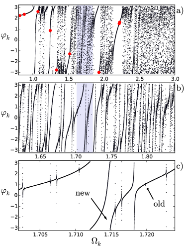
Figure 1: Snapshot of passive oscillators (black dots) and active oscillators (large red dots) phases plotted against natural frequencies for a finite ensemble of $50$ active oscillators (not all shown). The mean field is created by the active oscillators with natural frequencies drawn randomly from a Gaussian distribution (same sample as in Fig. 2) at slightly super-critical coupling $\varepsilon=1.85$ (same in Fig. 2). Three zoom levels of factor $10$ are marked by shaded areas. Arrows in c) point at $\Omega_{k}\approx 1.7145$ and $\Omega_{k}\approx 1.72$ for a new and an old phase slips, respectively. See Supplementary Material at [URL will be inserted by publisher] for an animated version of this figure. One second in the video equals one time unit.

First, we give a qualitative picture of the cross-correlations. Fig. 1 shows a snapshot of phases for a population of $N=50$ active oscillators together with a set of $M=5\cdot 10^{4}$ tracers. The natural frequencies of the active ones are sampled from a normal distribution with zero mean and unit variance, for which the critical coupling constant in the thermodynamic limit is $\varepsilon_{c}\approx 1.6$. The micro-scale ordering effect becomes evident if one zooms in to increasingly smaller scales, from panel a) to panel c). Panel c) shows the characteristic correlated state profile of the tracers’ phases, consisting of ruptured nearly horizontal bars. A bar is formed due to the ordering action of the fluctuations of the mean field, which synchronize passive oscillators with close frequencies. Ruptures appear when oscillators with higher frequencies make an additional rotation (a phase slip) with respect to oscillators with smaller (but similar) frequencies. In Fig. 1c) one can clearly see a fresh phase slip around $\Omega\approx 1.7145$, an older less pronounced phase slip around $\Omega\approx 1.717$, and several old phase slips that have almost disappeared. The phase slips become less visible over time because of the stabilizing effect reflected in a negative Lyapunov exponent as outlined above.

The micro-correlated structures like Fig. 1c) are observed in all disordered domains visible in the global picture Fig. 1a). Additionally, macroscopically ordered regions are seen close to the active oscillators not entrained by the mean field (with $\Omega_{k}\gtrsim 1.0$) (Fig. 1a). Here the tracers are synchronized to the active units (like the satellites are trapped by their planet’s gravitational field). This is because the fluctuations of the mean field are in fact not completely random, but contain relatively strong nearly periodic components from the non-entrained active oscillators. These components suffice, at least for small ensembles, to fully entrain tracers with natural frequencies close to a common active oscillator.

Figure 2: Observed cross-correlation as defined by Eq. (3) of passive oscillators coupled to the mean field $Z$ of $50$ active oscillators against their natural frequencies (mean $\langle R\rangle=0.58$, variance $\sigma_{R}^{2}=3.5\cdot 10^{-3}$), shown for various levels of frequency mismatch $\Delta$ between passive oscillators. a): Absolute value of the (time-averaged) first harmonic of individual passive oscillators before ($z$, blue circles) and after ($z_{\psi}$, red squares) the Möbius transform. $z_{\psi}$ drops to near zero after the transformation, which shows that $\psi$ is now uniformly rotating. b): Observed vs. natural frequencies of passive (line) and active oscillators (dots). Gray vertical lines in panels b), c) mark the natural frequencies of the active oscillators. c): Synchronization index $\gamma$ between pairs of passive oscillators with natural frequencies $\Omega_{k}\pm\Delta/2$.

Now we quantify the cross-correlations illustrated in Fig. 1. We calculate the cross-correlation coefficient $\gamma(\Omega,\Delta)$ for two tracers with natural frequencies $\Omega-\Delta/2,\,\Omega+\Delta/2$ according to (3). To this end, we need to perform the Möbius transformation (2) to obtain uniformly distributed phase variables $\psi$. First, we calculate the time dependent difference between the tracer phases and the mean field phase $\tilde{\varphi}(t)=\varphi(t)-\Phi(t)$. We then average these phases over time, $z=\langle\exp[i\tilde{\varphi}]\rangle$, which gives the empirical value of the parameter characterizing the wrapped Cauchy distribution of $\tilde{\varphi}$. Then, the Möbius transform (2) is applied. To check that we indeed obtained the uniformly distributed phase variable $\psi$, we calculate the first harmonics $z_{\psi}=\langle\exp[i\psi]\rangle$ and compare it to $z$ (Fig. 2a): one can see that indeed the transformation yields a uniformly distributed set of phase variables (within reasonable tolerance), because the amplitudes of the time averages of their first harmonics become very close to zero after the transformation.

In Fig. 2 b) we show the observed frequencies of the tracers and the active oscillators. One can clearly see synchronized neighborhoods of active units as plateaus in this graph. Outside the plateaus, the tracers are not locked and their observed frequency varies continuously with their natural one. It is in these domains outside the plateaus, that the micro-scale cross-correlations can be observed and measured, as illustrated in Fig. 2 c). Here we show values of the cross-correlation coefficient $\gamma(\Omega,\Delta)$ for several values of frequency mismatch $\Delta$: cross-correlation is nearly perfect for $\Delta\lesssim 10^{-5}$, while for $\Delta\gtrsim 0.01$ the values of the coefficient typically do not exceed $0.5$.

III.3 Fluctuations below the synchronization transition

To show that the effect of microscopic cross-correlations occurs for subcritical values of coupling constant $\varepsilon$ as well, we present the calculations of the cross-correlations for an ensemble of $N=50$ oscillators with natural frequencies randomly sampled from the standard normal distribution, and $\varepsilon=1$ in Fig. 3. For this relatively small coupling, the complex mean field fluctuates around zero, see e. g. Peter and Pikovsky (2018). Therefore, a transformation of the phases to uniformly rotating ones ($\tilde{\varphi}\to\psi$) is unnecessary, contrary to the case of a non-vanishing mean field at stronger coupling (Figs. 1,  2). For better visibility of both high and low cross-correlations, we present in Fig. 3 the cross-correlation constant $\gamma(\Omega,\Delta)$ in linear and logarithmic scales. The multiple locked regions relate to the frequencies of active oscillators. The central region around $\Omega\approx 0$ corresponds to the frequency of a synchronous cluster that has already been formed by the oscillators at the center of the locking region, even though this cluster is still not large enough to ensure the existence of a macroscopic mean field. The figure shows that the microscopic cross-correlations are of a universal nature and can be observed both below and above the synchronization transition.

Figure 3: The cross-correlations of passive oscillators coupled to a mean field of $50$ active ones at $\varepsilon=1$ (same natural frequency sample as Fig. 2). The mean field $Z$ fluctuates around zero, see Peter and Pikovsky (2018). Panel a): cross-correlations in the linear scale; panel b): the same in logarithmic scale to resolve the region $\gamma\lesssim 1$. Markers and colors as in Fig. 2 c).

\psfrag{xlab}[cc][cc]{$\log_{10}(d)$}\psfrag{ylab}[cc][cc]{$\gamma(d)$}\includegraphics[width=216.81pt]{fig4.eps}

Figure 4: Comparison of the observed cross-correlation $\gamma$ in sub- and super-critical ensembles ($\varepsilon=1$ and $1.85$ with open and filled symbols, respectively) of different sizes $N_{osc}=25,50,100,200$ with the theoretical expression (6) (solid line). The data points were generated in experiments as in Figs. 2, 3. The median of all $\gamma$’s for which $\gamma(10^{-2})<0.5$ (thereby excluding locked passive oscillators) is represented with error bars that mark the 25th and 75th percentile, respectively. Value $d=\Delta/\sigma^{2}$ is determined from the average over $\sigma^{2}=2\varepsilon^{2}D\{1+(|\Omega_{k}-\bar{\Omega}|/\Delta)^{2}\}$ with diffusion coefficient $D$ that was integrated from the auto-correlation function of $R$. For each ensemble size, only one set of natural frequencies is represented.

Finally, we illustrate in Fig. 4 a dependence of the cross-correlations on the noise level. Unfortunately, a quantitative comparison with the theoretical prediction (6) is not possible because the intrinsic fluctuations due to the finite-sized effect are very far from being delta-correlated, as is assumed in the analytical theory. Nevertheless, for a qualitative comparison, we calculated the autocorrelation function of the mean field, which has a peak at zero and pronounced oscillations due to the nearly periodic contributions of particular oscillators. As a measure of the effective noise intensity we took the difference $S$ between the peak value and the next largest maximum of the cross-correlations. This quantity decreases with the system size of the active ensemble. Furthermore, we have chosen only non-locked passive units. One can see that the scaling relation $\gamma=\gamma(\Delta/S)$ follows at least qualitatively the theoretical curve (6), although a huge diversity of the observed cross-correlations, due to the “coloredness” of the intrinsic finite-size mean field fluctuations, is also evident.

IV Conclusion

In summary, we have shown that the fluctuations of the mean field in the Kuramoto model, either externally imposed on the ensemble of infinite size, or naturally induced in the finite-sized model, lead to the appearance of cross-correlations in the disordered part of oscillator populations. These cross-correlations result from the competition between synchronization by common noise and desynchronization due to the parameter differences (usually the differences in the natural frequencies). We have developed an analytical theory of these cross-correlations for a mean field being a constant (in a properly rotating frame) plus additional Gaussian white noise, summarized in expression (6). This theoretical result is directly applicable to models similar to the Kuramoto model, e.g., to the Kuramoto-Sakaguchi model, where the mean field of a population is subject to external fluctuations. In the derivation of (6) we explicitly restrict the mean-field coupling to the first harmonics of the oscillator phases only. The case of a more general Daido-type coupling function requires extra analysis, although qualitative arguments imply that the cross-correlations will be observed there as well.

Furthermore, we have numerically characterized pairwise cross-correlations between passive oscillators driven by the intrinsically fluctuating mean fields in a finite ensemble at two different coupling strengths, super- and sub-critical, respectively. In both cases, the mean field contains nearly periodic components, therefore there exist locked regions where high values of pairwise cross-correlations arise due to resonant locking. Between these locked regions, the cross-correlations decay with increasing frequency mismatch, which is in a qualitative agreement with the theory based on white noise. The rather good quantitative agreement between white noise theory and finite Kuramoto model surprises, as, due to the dominant nearly periodic components in the fluctuating mean field, fluctuations in the finite Kuramoto model are far from being “white”.

Overall, the effect is expected to be most pronounced in situations where finite-size fluctuations are anomalously large (populations with equidistant natural frequencies at sub-critical coupling appear, as our preliminary calculations show, to belong to this class).

We expect that this phenomenon is not restricted to the mean-field coupling, and can be observed in other large systems where synchronized and disordered sub-populations coexist. A prominent example here is a chimera state in a one- or two-dimensional oscillatory medium with long-range interactions Kuramoto and Battogtokh (2002). A population of oscillators driven by two mean fields Zhang et al. (2017) also demonstrated nontrivial regimes with a coexistence of ordered and disordered subpopulations. Indeed, chimera states are defined as the coexistence of coherent and non-coherent domains among identical oscillators, and finite-size fluctuations Wolfrum and Omel’chenko (2011) may lead to cross-correlations in the disordered domain; this issue is currently under consideration.