Construction and Analysis of Posterior Matching in Arbitrary Dimensions via Optimal Transport

Abstract

The posterior matching scheme, for feedback encoding of a message point lying on the unit interval over memoryless channels, maximizes mutual information for an arbitrary number of channel uses. However, it in general does not always achieve any positive rate; so far, elaborate analyses have been required to show that it achieves any positive rate below capacity. More recent efforts have introduced a random “dither” shared by the encoder and decoder to the problem formulation, to simplify analyses and guarantee that the randomized scheme achieves any rate below capacity. Motivated by applications (e.g. human-computer interfaces) where (a) common randomness shared by the encoder and decoder may not be feasible and (b) the message point lies in a higher dimensional space, we focus here on the original formulation without common randomness, and use optimal transport theory to generalize the scheme for a message point in a higher dimensional space. By defining a stricter, almost sure, notion of message decoding, we use classical probabilistic techniques (e.g. change of measure and martingale convergence) to establish succinct necessary and sufficient conditions on when the message point can be recovered from infinite observations: Birkhoff ergodicity of a random process sequentially generated by the encoder. We also show a surprising “all or nothing” result: the same ergodicity condition is necessary and sufficient to achieve any rate below capacity. We provide applications of this message point framework in human-computer interfaces and multi-antenna communications.

I Introduction

Consider the communication problem shown in Figure 1: a message $W$ is signaled sequentially with feedback across a noisy channel. At time step $n$, an encoder uses the message $W$ and previous channel outputs $Y_{1},\ldots,Y_{n-1}$ to specify a signal $X_{n}$, which is then transmitted across the channel.

Motivated by emerging applications in human-computer interaction and the internet of things, we model the problem as $W\in{\mathsf{W}}\subset\mathbb{R}^{d}$ and consider optimizing over encoding strategies that map message point $W$ and previous channel outputs $Y_{1},\ldots,Y_{n-1}$ into the next channel input $X_{n}$. The decoder, with knowledge of the encoder’s strategy, simply performs Bayesian updates to sequentially construct a posterior belief $\psi_{n}$ about the message point after observations $Y_{1},\ldots,Y_{n}$. In this setup, we do not prespecify a block length; we can define reliability in terms of the message point $W$ being recoverable from all previous observations $Y_{1},Y_{2},\ldots$. This is equivalent to the condition that $\psi_{n}$ tends to a point mass at $W$. Secondly, we can define the notion of achieving a rate in terms of the speed of convergence of $\psi_{n}$ towards a point mass.

\begin{overpic}[width=433.62pt]{fig1-channelCodingFBnotext} \put(12.0,23.0){\bf causal} \put(12.0,19.0){\bf encoder} \put(72.0,23.0){\bf posterior} \put(72.0,19.0){\bf update} \put(39.0,23.0){\bf noisy} \put(39.0,19.0){\bf channel} \put(36.0,3.0){\bf delay} \put(91.0,24.0){\Large$\psi_{n}$} \put(59.0,24.0){\Large$Y_{n}$} \put(28.0,24.0){\Large$X_{n}$} \put(2.0,24.0){\Large$W$} \put(20.0,8.0){\Large$Y^{n-1}$} \put(2.0,8.0){$\mathbb{R}^{d}$} \end{overpic}

Figure 1: Communication of a message point $W$ with causal feedback over a memoryless channel. The message point $W$ lies in a continuum ${\mathsf{W}}\subset\mathbb{R}^{d}$ and it is our desire to optimize the encoder towards steering the posterior distribution on $W$ given $Y_{1},\ldots,Y_{n}$: $\psi_{n}$, towards a point mass at $W$ as rapidly as possible.

The posterior matching (PM) scheme recently developed by Shayevitz and Feder [1] is a feedback message point encoding scheme of this flavor when the message is a point on the unit interval, e.g. ${\mathsf{W}}=(0,1)$. It generalizes the scheme by Horstein that was specific to the binary symmetric channel [2], and the work of Schalkwijk and Kailath [3] that was specific to the additive noise Gaussian channel. The PM scheme has an iterative, time-invariant state space description, and maximizes mutual information. This is desirable for implementation because:

• The scheme does not have a pre-specified block length; it operates sequentially and at each time horizon, it maximizes the mutual information between the message point and all causal channel outputs.

• There is no forward error correction - it simply adapts on the fly and sequentially “hands the decoder what is missing”.

• The scheme admits a simple time-invariant dynamical system structure.

It can be interpreted as the optimal solution to an interactive two-agent sequential decision-making problem consisting of a Markov source process, a causal encoder with feedback, and a causal decoder [4].

However, from an information theoretic perspective, maximizing mutual information is necessary but not sufficient to achieve any rate below capacity. Indeed, examples have been shown [5] for which no positive rate can be achieved for the PM scheme. This has led to ‘regularity’ conditions imposed on the induced joint distribution between channel inputs and outputs to suffice for achieving any rate below capacity [1]. It is unclear if these conditions, which conceptually guarantee that the channel law is not too sensitive to perturbations on the channel input, are strictly required to achieve any rate below capacity. Moreover, motivated by human-computer interfaces [6, 7] and other applications, it would be desirable to have a problem formulation and solution, where the message point is in higher dimensions (e.g. ${\mathsf{W}}\subset\mathbb{R}^{d}$), that maintains the same iterative-time-invariant encoding properties as well as sufficient conditions on achieving any rate below capacity.

In their concluding remarks, Shayevitz and Feder discussed extending the posterior matching scheme to channels with memory, and in doing so, argued that a multidimensional message point would be required. They gave a conceptual example based on a Markovian channel of order $d$, which would require a $d+1$ dimensional message point in order to provide the “necessary degrees of freedom in terms of randomness”[1, Section VIII].

In what follows, we formulate a generalization to the message point feedback communication problem for higher dimensions and develop a posterior matching scheme with optimal transport theory that inherits all the desirable properties of the one-dimensional scheme. We use classical probabilistic techniques (e.g. change of measure and martingale convergence) to establish succinct necessary and sufficient conditions on achieving capacity: Birkhoff ergodicity of a random process sequentially generated by the encoder.

I-A Previous and Related Work

Horstein first introduced a problem of this framework for the binary symmetric channel (BSC) [2], where the message point lies on the $(0,1)$ interval. In this work, Horstein showed that the median of the posterior distribution is a sufficient statistic for the decoder to provide the encoder, for which the subsequent channel input signals whether the message point is larger or smaller than this threshold. Subsequently, Schalkwijk and Kailath [3][8] considered signaling a message point on the $(0,1)$ interval over the additive white Gaussian channel (AWGN) with feedback. There, they showed a close connection with estimation theory, where the minimum mean square error (MMSE) estimate of the message given all the observations plays a key role in the feedback encoder scheme. It was also shown that not only can capacity be achieved, but also a doubly exponential error exponent.

Shayevitz and Feder introduced the posterior matching scheme for the message point lying on the $(0,1)$ interval in [1] that is applicable to any memoryless channel. It includes the encoding schemes for the BSC and AWGN channel by Horstein and Schalkwijk-Kailath as special cases and provides the first rigorous proof that the Horstein scheme achieves capacity on the BSC.

Applications and variations of this formulation are manyfold. The Horstein scheme, combined with arithmetic coding of a sequence of symbols in an ordered symbolic alphabet to represent any sequence with enumerative source encoding [9] as a message point on the $(0,1)$ line, has been used for brain-computer interfaces to specify a sentence or a smooth path [10], to navigate mobile robots [11], and to remotely teleoperate an unmanned aircraft [6]. Many active learning problems borrow principles from posterior matching, but with different formulations or performance criteria; generalized 20 questions for target search [12, 13] and generalized binary search for function search [14, 15] serve as examples. Naghsvar and Tavidi considered variable-length encoding with feedback and utilized principles from stochastic control and posterior matching to demonstrate non-asymptotic upper bounds on expected code length and deterministic one-phase coding schemes that achieve capacity and attain optimal error exponents [16]. More general variable-length formulations of active hypothesis testing, where the statistics of the measurement may depend on the query or are controllable, have been developed in [17, 18, 19, 20]. Feedback coding channels with memory using principles from posterior matching have been explored in [21, 22, 23, 24].

Although the PM scheme maximizes mutual information, in some situations the posterior $\psi_{n}$ never converges to a point mass at $W$, implying that no positive rate is achievable. [1, Example 11] shows that the breakdown of reliability or achieving capacity is not solely a property of the channel: for the same channel, variants of the original scheme involving measure-preserving transformations of the input can ameliorate these issues. Sufficient conditions for reliability [1, Lemma 13] and achieving capacity [1, Theorem 4] were originally established in [1], involving ‘regularity’ and uniformly bounded max-to-min ratios assumptions along with elaborate fix-point analysis. This has led researchers to slightly alter the problem formulation and encoding schemes to more simply confirm guarantees on subsequent performance. Li and El Gamal [25] considered a non-sequential, fixed-rate, fixed-block-length feedback coding scheme for discrete memoryless channels (DMCs) when ${\mathsf{W}}=(0,1)$ and introduced a random dither known to the encoder and decoder to provide a simple proof of achieving capacity.

Also, Shayevitz and Feder [26] examined a randomized variant of the original PM scheme with a random dither and were able to provide a much simpler proof of optimality over general memoryless channels when $W\in(0,1)$. That is, as compared to the proofs above which are restricted to non-sequential variants with a fixed number of messages and only apply to DMCs, Shayevitz and Feder [26] used a random dither to provide a proof of optimality of the sequential, horizon-free, randomized posterior matching scheme over general memoryless channels. These settings where the encoder and decoder share a common source of randomness by way of a dither, however, may be undesirable in some situations (e.g. when considering human involvement as described above).

Recently, we have considered the case when the message point lies in a higher dimensional space (e.g. ${\mathsf{W}}\subset\mathbb{R}^{d}$ for some arbitrary $d$) and constructed a feedback encoding scheme using optimal transport theory [27]. Inspired by the time-invariant dynamical systems structure of the original PM scheme (without shared randomness at the encoder), and motivated by communication applications where humans play a role, below we develop appropriate notions of reliability and rate achievability in the multidimensional message point setting involving almost sure convergence. This allows us to use classical probability tools, including change of measure and martingale convergence, that have recently been employed by Van Handel to provide rigorous and succinct results pertaining to filter stability in hidden Markov models [28, 29], to provide succinct necessary and sufficient conditions for the generalized PM scheme to attain optimal performance. This provides a clear characterization of optimality of the original PM scheme in arbitrary dimensions in terms of Birkhoff ergodicity of an appropriate random process, without requiring the use of a dither.

I-B Main Contribution

In this paper, we address two unmet needs:

• We develop a generalization to the PM scheme for arbitrary memoryless channels where ${\mathsf{W}}\subset\mathbb{R}^{d}$ for any $d\geq 1$. Specifically, using optimal transport theory [30], we develop recursive encoding schemes that share the same mutual-information maximizing and iterative, time-invariant properties; moreover, they reduce to that of Shayevitz and Feder [1] when ${\mathsf{W}}=(0,1)$ as a special case.

• We define notions of reliability and achievability in a manner analogous to [1] but in terms of almost-sure convergence of random variables. With this, we then develop necessary and sufficient conditions for the scheme to be reliable and/or attain optimal convergence rate (e.g. achieve capacity). We show that both of these conditions have the same necessary and sufficient condition: the Birkhoff ergodicity of a random process $({\tilde{W}}_{n})_{n\geq 1}$ within the encoder of a PM scheme.

Optimal transport theory, used to construct schemes in (a), is also exploited in (b) where an invertibility property implicit in these schemes is used to show the equivalent conditions in (b). The rest of the paper is organized as follows:

In Section II, we provide definitions, terminology, and notations that will be used throughout the paper.

In Section III, we formulate the message point feedback communication problem for general memoryless channels, define the performance measure of reliability and of a rate being achievable, both in terms of almost-sure equivalents of the notions developed by Shayevitz & Feder [1]. We also provide necessary conditions for reliability of any message feedback encoder in terms of total variation convergence between two posterior distributions on the message point having the same observations but with different priors on ${\mathsf{W}}$ (Theorem III.7). We also discuss how this necessary condition and its proof are intimately related to results of Van Handel [29] on filter stability of hidden Markov models.

In Section IV, we define posterior matching schemes in arbitrary dimensions as time-invariant dynamical systems for an intermediate encoder state variable ${\tilde{W}}_{n}=S_{Y_{n-1}}({\tilde{W}}_{n-1})$ where the channel input satisfies $X_{n}=\phi({\tilde{W}}_{n})$. These schemes maximize $I(W;Y_{1},\ldots,Y_{n})$ for every $n\geq 1$ and satisfy a reliability necessary condition, developed in Lemma  IV.8, that $W\equiv{\tilde{W}}_{1}$ can be recovered from ${\tilde{W}}_{n+1}$ and $Y_{1:n}$ for any $n\geq 1$. We then show in Theorem IV.14 a collection of properties that PM schemes share, including the stationary and Markov nature of the random processes $({\tilde{W}}_{n})_{n\geq 1}$ and $({\tilde{W}}_{n},Y_{n})_{n\geq 1}$. We then demonstrate in Theorem IV.18 and Corollaries IV.21 and IV.23, via the theory of optimal transport, that we can use optimization approaches to explicitly and uniquely construct such PM schemes.

In Section V, we demonstrate in Theorem V.2 that the necessary and sufficient condition for reliability of the PM scheme is the Birkhoff ergodicity of the random process $({\tilde{W}}_{n})_{n\geq 1}$. This theorem uses the unique invertibility and statistical independence properties of the PM scheme along with classical probabilistic techniques such as martingale convergence and Blackwell & Freeman’s equivalent conditions on Birkhoff ergodicity of stationary Markov chains [31, Thm 2].

In Section VI, we show that three things are equivalent: (a) the PM scheme is reliable; (b) the random process $({\tilde{W}}_{n})_{n\geq 1}$ is ergodic; and (c) the PM scheme achieves any rate below capacity. This gives rise to an “all-or-nothing” property for PM schemes: ergodicity of the random process $({\tilde{W}}_{n})_{n\geq 1}$ elucidates essentially everything about the PM scheme’s performance: either no bits can be reliably transmitted (e.g. reliability does not hold), or any rate below capacity is achievable. The proofs involve the notion of “pullback intervals” developed by Shayevitz & Feder in [1], the construction of an auxiliary probability measure for which the logarithm of an appropriate Radon-Nikodym derivative is the information density, and classical probabilistic techniques including change of measure, martingale convergence, and stationarity of Markov chains.

In Section VII, we discuss applications in brain-computer interfaces and multi-antenna communications, and in Section VIII we provide some discussion and concluding remarks.

II Definitions and Notations

II-A Probability Definitions

• Denote $a_{i}^{j}$ as $(a_{i},\ldots,a_{j})$ and $a^{j}\triangleq a_{1}^{j}$. We also use $a_{i:j}$ and $a^{j}_{i}$ interchangeably.

• Denote $\mu$ as the Lebesgue measure on the Borel space for $\mathbb{R}^{d}$.

• Denote a probability space as $(\Omega,{\cal F},\mathbb{P})$ and the set of all probability measures on a measurable space $({\mathsf{X}},{\cal F}_{\mathsf{X}})$ as $\mathcal{P}\left({\mathsf{X}}\right)$.

• A transition kernel on ${\cal F}_{\mathsf{Y}}\times{\mathsf{X}}$ is a mapping $P_{Y|X}(\cdot|\cdot):{\cal F}_{\mathsf{Y}}\times{\mathsf{X}}\to[0,1]$, such that $P_{Y|X}(\cdot|x)\in\mathcal{P}\left({\mathsf{Y}}\right)$ for every $x\in{\mathsf{X}}$ and $P_{Y|X}(A|\cdot)$ is measurable for every $A\in{\cal F}_{\mathsf{Y}}$. For all $B\in{\cal F}_{\mathsf{Y}}$, define the marginal distribution $P_{Y}\in\mathcal{P}\left({\mathsf{Y}}\right)$ by

  $$P_{Y}(B) \equiv\int_{{\mathsf{X}}}P_{Y|X}(B|x)P_{X}(dx).$$

• Define the join on two $\sigma$-algebras $\mathcal{A}$ and $\mathcal{B}$, given by $\mathcal{A}\vee\mathcal{B}$, as the ​smallest $\sigma$-algebra containing both:

  $$\mathcal{A}\vee\mathcal{B}=\left\{A_{i}\cap B_{j}:A_{i}\in\mathcal{A},B_{j}\in\mathcal{B}\right\}$$

• Denote $\sigma(Y)$ as the sigma-algebra generated by random variable $Y$ and $\sigma(Y_{k},\ldots,Y_{m})$ as

  $$\sigma(Y_{k},\ldots,Y_{m})\triangleq\bigvee_{j=k}^{m}\sigma(Y_{j}).$$

  We use $\sigma(Y_{k},\ldots,Y_{m})$ and ${\cal F}^{Y}_{k,m}$ interchangeably.

II-B Information Theoretic Definitions

• We define the KL divergence as

  $$D\left(P\|Q\right)\equiv\begin{cases}{\mathbb{E}}_{P}[\log(dP/dQ)],&\text{if }P\ll Q\\ +\infty,&\text{otherwise }\end{cases}$$

• For $P_{X,Y}\in\mathcal{P}\left({\mathsf{X}\times{\mathsf{Y}}}\right)$ with marginals $P_{X}$ and $P_{Y}$, the information density is given by [32]:

  $$i(x,y) \triangleq\log\frac{dP_{X,Y}}{d(P_{X}\times P_{Y})}(x,y).$$ (1)

  The mutual information is defined as

  $$I(X;Y) \triangleq{\mathbb{E}}[i(X,Y)].$$ (2)

II-C Definitions for Birkhoff Ergodicity of Random Processes

• For two probability measures $P,Q$ defined on $\left({\mathsf{X}},{\cal F}\right)$ with densities with respect to the Lebesgue measure $\mu$ given by $p,q$, define the total variation distance $\|P-Q\|$ as:

  $$\|P-Q\|\triangleq \sup_{A\in{\cal F}}\left|P(A)-Q(A)\right|$$ (3)

• For a time-homogeneous Markov process $(V_{n})_{n\geq 1}$, denote $\mathbb{P}_{\nu}$ as the distribution on $(V_{n})_{n\geq 1}$ with $P_{V_{1}}=\nu$.

• For a random process $(V_{n})_{n\geq 1}$ on $(\Omega,{\cal F},\mathbb{P})$, the tail

  $$\mathcal{T}_{V}\triangleq\bigcap_{n\geq 1}\sigma(V_{n:\infty})$$

  is $\mathbb{P}$-trivial if $\mathbb{P}(E)=0$ or $\mathbb{P}(E)=1$ for any $E\in\mathcal{T}_{V}$.

• A stationary Markov process $(V_{n})_{n\geq 1}$ on a probability space $(\Omega,{\cal F},\mathbb{P})$ is defined as $\mathbb{P}$-ergodic when $\mathcal{T}_{V}$ is $\mathbb{P}$-trivial.

• A stationary Markov process $(V_{n})_{n\geq 1}$ on $(\Omega,{\cal F},\mathbb{P})$ with invariant measure $\nu$ on $({{\mathsf{V}}},{\cal F}_{{\mathsf{V}}})$ is denoted to be $\mathbb{P}$-mixing (in the ergodic theory sense) if for any $A,B\in{\cal F}_{\mathsf{V}}$:

  $$\lim_{n\to\infty}\mathbb{P}\left(V_{n}\in A,V_{1}\in B\right)=\nu(A)\nu(B).$$

• Lemma II.1 (Sec 2.5,[33])

  If a stationary Markov process $(V_{n})_{n\geq 1}$ is $\mathbb{P}$-mixing then it is $\mathbb{P}$-ergodic.

II-D Definitions for Optimal Transport Theory

• For $u\in\mathbb{R}^{d}$ and $M$ a $d$-by-$d$ positive definite matrix, denote the $M$-weighted Euclidean norm as $\|u\|_{M}^{2}=u^{T}Mu$.

• For ${\mathsf{W}}\subset\mathbb{R}^{d}$ and ${\cal F}_{{\mathsf{W}}}$ its Borel sets, consider two probability measures $P,Q\in\mathcal{P}\left({\mathsf{W}}\right)$. We say that a Borel-measurable map $S:{\mathsf{W}}\to{\mathsf{W}}$ pushes $P$ to $Q$, specified as $S\#P=Q$, if a random variable $W$ with distribution $P$ results in the random variable $V\equiv S(W)$ having distribution $Q$.

• Definition II.2

  A map $S:{\mathsf{W}}\to{\mathsf{W}}$ is a diffeomorphism if $S$ is invertible, $S$ is differentiable, and $S^{-1}$ is differentiable.

III The Message Point Feedback Communication Problem

III-A System Description

We consider the communication of a message point $W\in{\mathsf{W}}$ over a memoryless channel with causal feedback, as given in Figure 1.

We make the following assumption:

Assumption III.1

${\mathsf{W}},{\mathsf{X}},{\mathsf{Y}}$ each are Euclidean spaces with Borel sigma-algebras and ${\mathsf{W}},{\mathsf{X}}\subset\mathbb{R}^{d}$. Moreover, ${\mathsf{W}}$ is open, bounded and convex.

Our notion of a communication system in Figure 1 is somewhat non-traditional because (a) we do not a priori specify the number $n$ of channel uses and (b) by virtue of Assumption III.1, ${\mathsf{W}}$ is a continuous rather than discrete set of possible messages.

The encoder policy $\Psi=(e_{n}:{\mathsf{W}}\times{\mathsf{Y}}^{n-1}\to{\mathsf{X}})_{n\geq 1}$ specifies the next channel input $X_{n}=e_{n}(W,Y^{n-1})$. The channel input $X_{n}\in{\mathsf{X}}$ is passed through a time-invariant memoryless channel to produce $Y_{n}\in{\mathsf{Y}}$:

$$\mathbb{P}\left(Y_{n}\in A|\sigma(X_{1:\infty},Y_{1:n-1})\right)=P_{Y|X}(A|X_{n}).$$ (4)

Definition III.2

Define $P_{W}\equiv\bar{\nu}$ as the uniform distribution on ${\mathsf{W}}$. We will consider two cases, $W\sim\bar{\nu}$, and also when $W\sim\nu$, where $\nu\ll\bar{\nu}$ but is otherwise arbitrary.

Given the distribution $\nu~{}(\bar{\nu})$ on the message point $W$, the policy $\Psi=(e_{n}:{\mathsf{W}}\times{\mathsf{Y}}^{n-1})_{n\geq 1}$ and the channel $P_{Y|X}$, denoted succinctly as $\left(\nu,\Psi,P_{Y|X}\right)$ $\left(\left(\bar{\nu},\Psi,P_{Y|X}\right)\right)$ respectively, the full distribution on $\left(W,(X_{n})_{n\geq 1},(Y_{n})_{n\geq 1}\right)$ is specified. For any encoder policy $\Psi$ and given channel $P_{Y|X}$, we will always consider two probability spaces:

• $(\Omega,{\cal F},\mathbb{P})$ pertaining to $\left(\nu,\Psi,P_{Y|X}\right)$.

• $(\Omega,{\cal F},\mathbb{\overline{P}})$ pertaining to $\left(\bar{\nu},\Psi,P_{Y|X}\right)$.

Since ${\mathsf{W}},{\mathsf{X}},{\mathsf{Y}}$ are countably generated, a regular version of the posterior distribution $\psi_{n}~{}(\bar{\psi}_{n})$ on $W$ given $Y_{1:n}$ exists under $\mathbb{P}~{}(\mathbb{\overline{P}})$, respectively. Let $\lambda_{Y}$ be a $\sigma$-finite (reference) measure on ${\mathsf{Y}}$ so that $P_{X_{n},Y_{n}}\ll P_{X_{n}}\otimes\lambda_{Y}$, and define $L(y|x)\triangleq\frac{dP_{Y_{n}|X_{n}=x}}{d\lambda_{Y}}(y)$. Then we can describe the recursive update to $\psi_{n}~{}(\bar{\psi}_{n})$, which satisfies a recursive update equation pertaining to Bayes’ rule. Specifically, for any $A\in{\cal F}_{\mathsf{W}}$, we have:

$$\psi_{n}(A) \triangleq \mathbb{P}\left(W\in A|{\cal F}^{Y}_{1:n}\right)$$ (5a)

$$\bar{\psi}_{n}(A) \triangleq \mathbb{\overline{P}}\left(W\in A|{\cal F}^{Y}_{1:n}\right)$$ (5b)

As noted in Definition III.2, $P_{W}$ will always indicate $\bar{\nu}$, the uniform distribution on ${\mathsf{W}}$ for the remainder of the manuscript, and $(\Omega,{\cal F},\mathbb{\overline{P}})$ will be the probability space for which all formal performance criteria will be evaluated. $\nu\ll\bar{\nu}$ and the associated probability space $(\Omega,{\cal F},\mathbb{P})$ will be defined in a context-specific manner for certain theorems (Theorem III.7, Lemma V.1) and their proofs (Theorem V.2).

Remark III.3

Our rationale for making the definitions of $\bar{\nu}$ and $\nu$ along with $\mathbb{P}$ and $\mathbb{\overline{P}}$ will become clearer in Section V: it allows us to be notationally consistent with definitions used in the analysis of nonlinear filter stability, which explores when the posterior distribution in a hidden Markov model is sensitive to the initial distribution on the state variable (e.g. $\nu$ vs $\bar{\nu}$) [28]. One key difference, however, is that the nonlinear filter pertains to recursive updates of the posterior distribution of the current latent state of a hidden Markov model. In our setting, our focus is squarely on recursively updating $\psi_{n}$ and $\bar{\psi}_{n}$, the posterior distribution on the latent initial condition $W$.

III-B Reliable Communication

We now provide a formalism of achievability that implies the standard Shannon theoretic notions in [34].

Definition III.4 (Reliability)

An encoder policy $\Psi$ is reliable if $W$ is ${\cal F}^{Y}_{1:\infty}$-measurable $\mathbb{\overline{P}}-a.s.$

In other words, reliability means that from all the observations $(Y_{n})_{n\geq 1}$, one can perfectly reconstruct $W$. This implies that any fixed number of bits can be decoded from all the measurements. Because the number of decodable messages does not grow with the number of channel usages $n$, we can analogously say that this means achieving “zero rate”. Figure 2 shows the posterior distribution trajectory of two encoding schemes, one that is reliable and another that is not.

\begin{overpic}[width=433.62pt]{fig2-rateDefv3} \put(30.0,55.0){ $\bar{\psi}_{0}(\cdot)$} \put(30.0,20.0){ $\bar{\psi}_{0}(\cdot)$} \put(85.0,30.0){ $\bar{\psi}_{n}(\cdot)$} \put(85.0,70.0){ $\bar{\psi}_{n}(\cdot)$} \end{overpic}

Figure 2: (a) represents prior $\bar{\psi}_{0}$, (b) represents the posterior $\bar{\psi}_{n}$ after observations $y^{n}$ when the scheme is unreliable. (c) and (d) show the same as (a) and (b) respectively, except the scheme is reliable.

III-C Reliable Communication at rate R

We now provide a definition of achieving a rate $R$ that implies the standard Shannon theoretic notions in [34].

Definition III.5 (Rate)

An encoder policy $\Psi$ achieves rate $R$ if, given any $\epsilon\in(0,1)$, there exists a sequence of Borel sets $(A_{n}^{\epsilon})_{n\geq 1}$ for which:

1. $A_{n}^{\epsilon}$ is open and convex for each $n\geq 1$,   $\mathbb{\overline{P}}-a.s.$

2. $\Psi$ is reliable.

3. $\underset{n\to\infty}{\liminf}\bar{\psi}_{n}(A_{n}^{\epsilon})\geq 1-\epsilon\quad\mathbb{\overline{P}}-a.s.$

4. $\underset{n\to\infty}{\liminf}-\frac{1}{n}\log\bar{\nu}(A_{n}^{\epsilon})\geq R\quad\mathbb{\overline{P}}-a.s.$

Remark III.6

For ${\mathsf{W}}=(0,1)$, property (i) is equivalent to $A_{n}$ being an open interval [35], thus generalizing the definition of a decoded interval in [1] to arbitrary dimensions. Whereas achievability of a rate $R$ for PM was defined by Shayevitz & Feder in terms of the normalized volume and posterior probabilities convergence probability (c.f. [1, Equation (2)]), conditions in (iii) and (iv) given here are in terms of almost sure convergence. Since the Shayevitz & Feder notion of achievability of a rate $R$ implies that of the standard coding framework [1, Lemma 3], and since almost sure convergence implies convergence in probability, Definition III.5 also implies achievability in the standard coding sense.

We now provide a necessary condition for any encoding scheme $\Psi$ to be reliable, which leverages recent intrinsic methods in filter stability for hidden Markov models [29]; this will be used later in the manuscript:

Theorem III.7

If an encoding scheme $\Psi$ is reliable, then

$$\lim_{n\to\infty}{\mathbb{E}}_{\nu}\left[\left\|\psi_{n}-\bar{\psi}_{n}\right\|\right]=0$$

for any $\nu\ll\bar{\nu}$.

Proof:

This follows closely the derivation of equation 1.9 in [29]. From (5), for any fixed measures $\nu$ and $\bar{\nu}$ s.t. $\nu\ll\bar{\nu}$, $\psi_{0}=\nu$ and $\bar{\psi}_{0}=\bar{\nu}$, $\frac{d\mathbb{P}}{d\mathbb{\overline{P}}}=\frac{d\nu}{d\bar{\nu}}(W).$ From Bayes’ rule, for any non-negative measurable function $g:{\mathsf{W}}\to\mathbb{R}^{+}$ the following holds,

$${\mathbb{E}}_{\nu}\left[g(W)|{\cal F}^{Y}_{1:n}\right] =\frac{{\overline{\mathbb{E}}}\left[g(W)\frac{d\mathbb{P}}{d\mathbb{\overline{P}}}\Big{|}{\cal F}^{Y}_{1:n}\right]}{{\overline{\mathbb{E}}}\left[\frac{d\mathbb{P}}{d\mathbb{\overline{P}}}\Big{|}{\cal F}^{Y}_{1:n}\right]}$$

$$=\frac{\int_{{\mathsf{W}}}g(w)\frac{d\nu}{d\bar{\nu}}(w)\bar{\psi}_{n}(dw)}{{\overline{\mathbb{E}}}\left[\frac{d\nu}{d\bar{\nu}}(W)\Big{|}{\cal F}^{Y}_{1:n}\right]}$$

$$\Rightarrow\frac{d\psi_{n}}{d\bar{\psi}_{n}}(W) =\frac{\frac{d\nu}{d\bar{\nu}}(W)}{{\overline{\mathbb{E}}}\left[\frac{d\nu}{d\bar{\nu}}(W)\Big{|}{\cal F}^{Y}_{1:n}\right]}$$

Thus we have that the following holds $\mathbb{P}_{\nu}$ almost surely:

$$\left\|\psi_{n}-\bar{\psi}_{n}\right\| =\int_{{\mathsf{W}}}\left|\frac{d\psi_{n}}{d\bar{\psi}_{n}}(w)-1\right|\bar{\psi}_{n}(dw)$$

$$=\frac{{\overline{\mathbb{E}}}\left[\left|\frac{d\nu}{d\bar{\nu}}(W)-{\overline{\mathbb{E}}}\left[\frac{d\nu}{d\bar{\nu}}(W)|{\cal F}^{Y}_{1:n}\right]\right|\big{|}{\cal F}^{Y}_{1:n}\right]}{{\overline{\mathbb{E}}}\left[\frac{d\nu}{d\bar{\nu}}(W)|{\cal F}^{Y}_{1:n}\right]}$$ (6)

Thus we have that

$${\mathbb{E}}_{\nu}\left[\left\|\psi_{n}-\bar{\psi}_{n}\right\|\right] ={\overline{\mathbb{E}}}\left[\frac{d\nu}{d\bar{\nu}}(W)\left\|\psi_{n}-\bar{\psi}_{n}\right\|\right]$$

$$={\overline{\mathbb{E}}}\left[{\overline{\mathbb{E}}}\left[\frac{d\nu}{d\bar{\nu}}(W)|{\cal F}^{Y}_{1:n}\right]\left\|\psi_{n}-\bar{\psi}_{n}\right\|\right]$$ (7)

$$={\overline{\mathbb{E}}}\left[\left|\frac{d\nu}{d\bar{\nu}}(W)-{\overline{\mathbb{E}}}\left[\frac{d\nu}{d\bar{\nu}}(W)|{\cal F}^{Y}_{1:n}\right]\right|\right]$$ (8)

where (7) follows from the tower law of expectation and the fact that ${\overline{\mathbb{E}}}\left[\frac{d\nu}{d\bar{\nu}}(W)|{\cal F}^{Y}_{1:n}\right]$ and $\left\|\psi_{n}-\bar{\psi}_{n}\right\|$ are ${\cal F}^{Y}_{1:n}$-measurable; and (8) follows from (6) and the tower law of expectation. The conditional expectation ${\overline{\mathbb{E}}}\left[\frac{d\nu}{d\bar{\nu}}(W)|{\cal F}^{Y}_{1:n}\right]$ in (8) is a nonnegative uniformly integrable martingale with respect to the increasing filtration ${\cal F}^{Y}_{1:n}$. Hence it converges in $L^{1}(\mathbb{\overline{P}})$ and we have

$$\lim_{n\to\infty}{\mathbb{E}}_{\nu}\left[\left\|\psi_{n}-\bar{\psi}_{n}\right\|\right]$$

$$={\overline{\mathbb{E}}}\left[\left|\frac{d\nu}{d\bar{\nu}}(W)-{\overline{\mathbb{E}}}\left[\frac{d\nu}{d\bar{\nu}}(W)|{\cal F}^{Y}_{1:\infty}\right]\right|\right]$$

$$=0$$ (9)

where (9) follows from the assumption that the PM scheme is reliable, thus implying that ${\overline{\mathbb{E}}}\left[\frac{d\nu}{d\bar{\nu}}(W)|{\cal F}^{Y}_{1:\infty}\right]=\frac{d\nu}{d\bar{\nu}}(W)$ from Definition III.4. ∎

IV Posterior Matching Schemes in Arbitrary Dimensions

In this section, we will introduce a simple feedback-based encoding scheme, termed the posterior matching (PM) scheme. The motivation is to satisfy some necessary conditions on achieving any possible rate. We start by discussing the properties that any feedback encoding scheme should have for it to maximize mutual information by looking at the converse to the feedback communication problem. We then show how the PM scheme in 1 dimension, developed by Shayevitz & Feder in [1], follows naturally and can be described in a dynamical system format. We then define a class of dynamical system encoders in arbitrary dimensions and provide a necessary condition on any such encoder to be reliable. With this necessary condition, we define posterior matching schemes in arbitrary dimensions, provide unique construction of PM schemes by optimal transport, and showcase a large number of properties that such schemes possess (e.g. stationary, Markov, etc).

All subsequent discussions assume the following:

Assumption IV.1

The capacity of the communication channel is finite, $I(P_{X}^{*},P_{Y|X})<\infty$.

With this, we have the following Lemma:

Lemma IV.2

Under Assumption IV.1, $P_{W|Y=y}\ll P_{W}$ for $P_{Y}$-almost all $y$. Moreover, $i(X;Y)$ is integrable.

Proof:

Now suppose that for some $P_{Y}$-nontrivial $y$, the absolute continuity condition $P_{W|Y=y}\ll P_{W}$ does not hold. Then clearly by definition, $D\left(P_{W|Y=y}\|P_{W}\right)=\infty$ and moreover,

$$\infty =\int_{{\mathsf{Y}}}D\left(P_{W|Y=y}\|P_{W}\right)P_{Y}(dy)$$

$$=I(W;Y)$$

$$=I(P_{X}^{*},P_{Y|X})$$

which is a contradiction. Therefore, according to the definition of the information density in (• ‣ II-B), $i(X;Y)$ is integrable. ∎

IV-A Maximizing Mutual Information

Given the channel $P_{Y|X}$ and a cost function $\eta:{\mathsf{X}}\to\mathbb{R}_{+}$, the capacity-cost function is given by

$$C\left(\eta,P_{Y|X},L\right)\triangleq\!\!\!\!\max_{P_{X}\in\mathcal{P}\left({\mathsf{X}}\right):{\mathbb{E}}_{P_{X}}\left[\eta(X)\right]\leq L}\!\!\!\!I(P_{X},P_{Y|X}).$$ (10)

It is known that $C\left(\eta,P_{Y|X},L\right)$ is the fundamental limit of communication over a channel $P_{Y|X}$ of all encoders whose average cost $\eta(X)$ is upper-bounded by $L$ [36].

We note the following standard lemma from information theory [34]:

Lemma IV.3

Fix an $n\geq 1$. If a feedback encoder $\left(X_{i}=e_{i}(W,Y^{i-1}):i=1,\ldots,n\right)$ satisfies the constraint

$${\overline{\mathbb{E}}}\left[\frac{1}{n}\sum_{i=1}^{n}\eta(X_{i})\right]\leq L,$$

then

$$\frac{1}{n}I(W;Y^{n})\leq C\left(\eta,P_{Y|X},L\right).$$

Equality holds if and only if

• $Y_{1},\ldots,Y_{n}$ are statistically independent.

• $X_{i}\sim P^{*}_{X}$ for each $i$, where $P^{*}_{X}$ is the capacity-achieving distribution in (10).

The original PM scheme for ${\mathsf{W}}=(0,1)$ developed by Shayevitz & Feder is given as follows.

Example IV.4 (PM Scheme in One Dimension [1])

Define $F_{X}(\cdot)$ as the CDF associated with $P_{X}^{*}$ above and

$$X_{n} =F_{X}^{-1}({\tilde{W}}_{n})\quad n\geq 1$$ (11)

$${\tilde{W}}_{1} =W,\quad{\tilde{W}}_{n+1}=F_{W|Y_{1:n}}(W|Y_{1:n}),\quad n\geq 1\;$$

where $F_{W|Y_{1:n}}(w|y_{1:n})$ is the conditional cumulative distribution function (CDF) of the message point $W$ given $n$ channel observations $Y_{1:n}$ under $(\Omega,{\cal F},\mathbb{\overline{P}})$, e.g. with $\bar{\nu}$ as the prior distribution on $W$. The intuition here is that by placing the message point into its own conditional CDF, this guarantees that the new state variable ${\tilde{W}}_{n+1}$ is uniformly distributed, for all $Y_{1:n}$; thus ${\tilde{W}}_{n+1}\sim\bar{\nu}$ and is independent of $Y_{1:n}$. Since $X_{n+1}$ is simply a function of ${\tilde{W}}_{n+1}$, it is still independent of $Y_{1:n}$; moreover, by defining it in terms of the inverse CDF of $P_{X}^{*}$, it also has the capacity-achieving distribution $P_{X}^{*}$. As such, this simple scheme guarantees that $I(W;Y_{1:n})=nC$ for all $n\geq 1$. In addition, ${\tilde{W}}_{n+1}$ is “handing the decoder what is missing”, because given $Y_{1:n}$, ${\tilde{W}}_{n+1}$ and $W$ form a bijection, by virtue of the monotonicity (and thus invertibility) of CDFs. It can be shown [1] that the one-dimensional PM scheme (11) can equivalently be written as

$$X_{n} =F_{X}^{-1}({\tilde{W}}_{n})\quad n\geq 1$$ (12)

$${\tilde{W}}_{1} =W,\quad{\tilde{W}}_{n+1}=F_{{\tilde{W}}|Y}({\tilde{W}}_{n}|Y_{n}),\;\;n\geq 1$$

where $F_{{\tilde{W}}|Y}(\cdot|y)$ is the CDF associated with the posterior distribution $P_{{\tilde{W}}_{1}|Y_{1}=y}$ of the message point ${\tilde{W}}_{1}$ given $Y_{1}=y$ under $(\Omega,{\cal F},\mathbb{\overline{P}})$, where $P_{W}=\bar{\nu}$ and $P_{Y|W}(dy|\tilde{w})\equiv P_{Y|X}\left(dy|F_{X}^{-1}(\tilde{w})\right)$.

When the one-dimensional posterior matching scheme is written in the format of (12), notice that $({\tilde{W}}_{n})_{n\geq 1}$ is a stochastic dynamical system where ${\tilde{W}}_{n+1}=S_{Y_{n}}({\tilde{W}}_{n})$ is controlled by the i.i.d. sequence of random variables $(Y_{n})_{n\geq 1}$, with $S_{y}(u)=F_{{\tilde{W}}|Y}(u|y)$.

IV-B Dynamical System Encoders

Inspired by the original one-dimensional PM scheme developed in [1], here we also consider dynamical systems $({\tilde{W}}_{n})_{n\geq 1}$ where ${\tilde{W}}_{n+1}=S_{Y_{n}}({\tilde{W}}_{n})$ and ${\tilde{W}}_{1}=W$ is the message. Moving forward, when describing dynamical system encoders, we do not restrict ourselves to ${\mathsf{W}}=(0,1)$; rather, we now consider the more general case where only Assumption III.1 holds.

Definition IV.5

A dynamical system encoder is a collection of maps $(S_{y}:{\mathsf{W}}\to{\mathsf{W}})_{y\in{\mathsf{Y}}}$ and a memoryless, time-invariant noisy channel with transition kernel $P_{Y_{n}|{\tilde{W}}_{n}}(\cdot|\cdot)\equiv P_{Y|{\tilde{W}}}(\cdot|\cdot)$. Their dynamics govern the random process $({\tilde{W}}_{n},Y_{n})_{n\geq 1}$ as follows:

$${\tilde{W}}_{1}=W,\quad{\tilde{W}}_{n+1}=S_{Y_{n}}({\tilde{W}}_{n}),\quad n\geq 1$$

The intuition here is that ${\tilde{W}}_{n}$ is signaled into the noisy channel to specify $Y_{n}$. At the next step, ${\tilde{W}}_{n+1}$ is governed by ${\tilde{W}}_{n}$ and the most recent channel output $Y_{n}$. As such, it is a time-invariant, memoryless stochastic dynamical system, as shown in Figure 3.

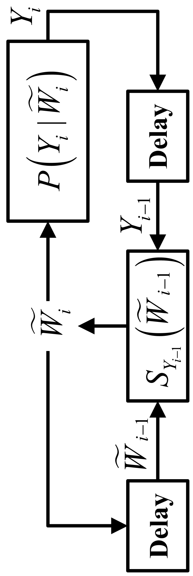
Figure 3: Dynamical system encoder as discussed in Definition IV.5 that underlies the posterior matching scheme.

The next two lemmas do not make an i.i.d. assumption on $(Y_{n})_{n\geq 1}$; rather, they elucidate basic Markov properties any dynamical system encoder possesses, and then provide a necessary condition, for any dynamical system encoder, for recovering the message $W$ from $(Y_{n})_{n\geq 1}$.

Lemma IV.6

For any dynamical system encoder, $(Y_{n},{\tilde{W}}_{n+1})_{n\geq 1}$ is a Markov process. Moreover, for any $n\geq 1$ the following Markov chain condition holds

$${\tilde{W}}_{1}\rightarrow(Y_{1:n},{\tilde{W}}_{n+1})\rightarrow(Y_{n+1:\infty},{\tilde{W}}_{n+2:\infty})$$ (13)

Proof:

We note that ${\tilde{W}}_{1}$ has initial distribution $P_{W}$. Note that $Y_{1}$ is ${\tilde{W}}_{1}$ being passed through a noisy memoryless channel, which is a stochastic kernel. As such, for appropriately defined functions $g_{1}$ and random variable $N_{1}$, we have that $Y_{1}=g_{1}({\tilde{W}}_{1},N_{1})$. Secondly, note that ${\tilde{W}}_{2}=S_{Y_{1}}({\tilde{W}}_{1})\equiv g_{2}({\tilde{W}}_{1},N_{1})$. This process continues onward.

Because the channel $P_{Y|X}$ is memoryless and time-invariant, this means that $N_{1},N_{2},\ldots$ are i.i.d. Thus $(Y_{n},{\tilde{W}}_{n+1})_{n\geq 1}$ is an iterated function system (IFS) controlled by $(N_{n})_{n\geq 1}$. An IFS is known to be a Markov process [37].

As such, we have that the following Markov chain condition holds:

$$(Y_{1:n-1},{\tilde{W}}_{1:n})\rightarrow(Y_{n},{\tilde{W}}_{n+1})\rightarrow(Y_{n+1:\infty},{\tilde{W}}_{n+2:\infty})$$

We state this equivalently in terms of conditional mutual information and the chain rule:

$$0 = I\left(Y_{1:n-1},{\tilde{W}}_{1:n};Y_{n+1:\infty},{\tilde{W}}_{n+2:\infty}|Y_{n},{\tilde{W}}_{n+1}\right)$$

$$= I\left(Y_{1:n-1};Y_{n+1:\infty},{\tilde{W}}_{n+2:\infty}|Y_{n},{\tilde{W}}_{n+1}\right)$$

$$+ I\left({\tilde{W}}_{1};Y_{n+1:\infty},{\tilde{W}}_{n+2:\infty}|Y_{1:n},{\tilde{W}}_{n+1}\right)$$

$$+ I\left({\tilde{W}}_{2:n};Y_{n+1:\infty},{\tilde{W}}_{n+2:\infty}|Y_{1:n},{\tilde{W}}_{1},{\tilde{W}}_{n+1}\right)$$

Since conditional mutual information is non-negative, it follows that all three terms must be zero. (IV-B) being zero is equivalent to the Markov chain condition (13). ∎

Definition IV.7

We say a dynamical systems encoder is invertible if ${\tilde{W}}_{1}$ is $\mathbb{\overline{P}}$-a.s. $\sigma({\tilde{W}}_{n+1},Y_{1:n})$-measurable $\;\forall n\geq 1$.

We now show a necessary condition on the structure of $(S_{y})_{y\in{\mathsf{Y}}}$ in order for an agent only observing $(Y_{n})_{n\geq 1}$ to be able to recover the initial condition ${\tilde{W}}_{1}$.

Lemma IV.8

If a dynamical encoding scheme is reliable, then it is invertible.

Proof:

Consider any measurable integrable function $g$. Note then that

$${\overline{\mathbb{E}}}\left[g({\tilde{W}}_{1})|Y_{1:n},{\tilde{W}}_{n+1}\right] ={\overline{\mathbb{E}}}\left[g({\tilde{W}}_{1})|Y_{1:\infty},{\tilde{W}}_{n+1:\infty}\right]$$ (15)

$$=g({\tilde{W}}_{1})$$ (16)

where (15) follows from Lemma IV.6; and (16) follows from the assumption of reliability and Definition III.4, implying that ${\tilde{W}}_{1}$ is $\mathbb{\overline{P}}$-a.s. ${\cal F}^{Y}_{1:\infty}$-measurable.

∎

Note that Lemma IV.8 indicates that in order for the message $W$ to be recoverable from $Y_{1:\infty}$, it must be that for any $n\geq 1$, $W$ is recoverable from ${\tilde{W}}_{n+1}$ and the feedback of the past channel outputs $Y_{1:n}$. This is analogous to a notion of invertibility defined by Van Handel for a different but related class of hidden Markov models [38, Defn 2.6, Remark 2.10]. This necessary condition on reliability will motivate our definition of the posterior matching scheme, defined in the next section, to have an invertible structure.

Lemma IV.6, we have that $(Y_{n},{\tilde{W}}_{n+1})_{n\geq 1}$ is a Markov chain and so we can define a hidden Markov model with state variable $V_{n}=(Y_{n},{\tilde{W}}_{n+1})$ and observation variable $Y_{n}$. Note that the posterior distribution on $V_{n}$ given $Y_{1:n}$ is fully captured by the posterior distribution on ${\tilde{W}}_{n+1}$ given $Y_{1:n}$, which we term $\pi_{n}$ ($\bar{\pi}_{n}$) under $\mathbb{P}_{\nu}$ ($\mathbb{\overline{P}}$), respectively. If a dynamical systems encoder is invertible, then note from Definition IV.7 that for any $A\in{\cal F}_{\mathsf{W}}$, there exists a ${\cal F}^{Y}_{1:n}$-measurable $B\in{\cal F}_{\mathsf{W}}$ for which $\mathbb{\overline{P}}\left({\tilde{W}}_{1}\in A|{\cal F}^{Y}_{1:n}\right)=\mathbb{\overline{P}}\left({\tilde{W}}_{n+1}\in B|{\cal F}^{Y}_{1:n}\right)$. If we replace the roles of ${\tilde{W}}_{1}$ and ${\tilde{W}}_{n+1}$, we arrive at an analogous statement; thus we have the following remark:

Remark IV.9

From (3), it follows that for any for any invertible dynamical systems encoder:

$$\|\pi_{n}-\bar{\pi}_{n}\|=\|\psi_{n}-\bar{\psi}_{n}\|.$$

Note that the fundamental question of filter stability for hidden Markov models involves understanding if the posterior distribution on the state variable at time $n$ becomes insensitive to the prior distribution on the initial state variable [29, eq 1.5]:

$$\lim_{n\to\infty}{\mathbb{E}}_{\nu}\left[\|\pi_{n}-\bar{\pi}_{n}\|\right]\stackrel{{\scriptstyle?}}{{=}}0\quad\forall\nu\ll\bar{\nu}.$$

We can combine the necessary condition for any encoding scheme $\Psi$ to be reliable in Theorem III.7 with the necessary condition for a dynamical systems encoder to be reliable in Lemma IV.8 to conclude that:

Corollary IV.10

For any invertible dynamical systems encoder, a necessary condition on reliability is that for any $\nu\ll\bar{\nu}$,

$$\lim_{n\to\infty}{\mathbb{E}}_{\nu}\left[\|\pi_{n}-\bar{\pi}_{n}\|\right]=0.$$

This clearly elucidates an intimate connection between the topic of filter stability for hidden Markov models and the topic of reliability for dynamical system encoding schemes for message-point feedback communication problems.

IV-C The Posterior Matching Scheme

We now define the posterior matching scheme for ${\mathsf{W}}\subset\mathbb{R}^{d}$ as a time-invariant dynamical system encoder that contains all the essential properties of the PM scheme for ${\mathsf{W}}=(0,1)$ developed by Shayevitz & Feder in [1].

Definition IV.11

A posterior matching (PM) scheme is a dynamical system encoder with the following properties:

$${\tilde{W}}_{1}=W,\quad{\tilde{W}}_{i}=S_{Y_{i-1}}({\tilde{W}}_{i-1}),\quad i\geq 1$$ (17a)

$$X_{i}=\phi({\tilde{W}}_{i})$$ (17b)

$$S_{y}\#P_{{\tilde{W}}_{1}|Y_{1}=y}=P_{W}\text{ invertibly }\quad\forall y\in{\mathsf{Y}},$$ (17c)

$$\phi\#P_{W}=P_{X}^{*}$$ (17d)

The invertibility of $S_{y}:{\mathsf{W}}\to{\mathsf{W}}$ for each $y\in{\mathsf{Y}}$ is inspired by the necessary condition of invertibility given in Lemma IV.8. This invertibility property implies that with knowledge of $Y_{1:n}$, not only can ${\tilde{W}}_{n+1}$ be constructed from ${\tilde{W}}_{1}$, but also that ${\tilde{W}}_{1}$ can be constructed from ${\tilde{W}}_{n+1}$:

$${\tilde{W}}_{n+1} =S_{Y_{1:n}}({\tilde{W}}_{1})\triangleq S_{Y_{n}}\circ\cdots\circ S_{Y_{1}}({\tilde{W}}_{1})$$ (18a)

$${\tilde{W}}_{1} =S^{-1}_{Y_{1:n}}({\tilde{W}}_{n+1})\triangleq S_{Y_{1}}^{-1}\circ\cdots\circ S_{Y_{n}}^{-1}({\tilde{W}}_{n+1})$$ (18b)

Below is a key lemma which conceptually shows that any PM scheme is “handing the decoder what is missing”:

Lemma IV.12

For any PM scheme, the following holds:

$$\mathbb{\overline{P}}\left({\tilde{W}}_{n+1}\in\cdot\big{|}{\cal F}^{Y}_{1:n}\right) =\mathbb{\overline{P}}\left(W\in\cdot\right),\quad\mathbb{\overline{P}}-a.s.$$ (19)

$$\mathbb{\overline{P}}\left({\tilde{W}}_{n}\in\cdot\big{|}{\cal F}^{Y}_{1:n}\right) =\mathbb{\overline{P}}\left({\tilde{W}}_{n}\in\cdot|Y_{n}\right)$$ (20)

Proof:

We show this by induction. First note that for $n=2$, we have that ${\tilde{W}}_{2}=S_{Y_{1}}({\tilde{W}}_{1})$. Now we note that given $Y=y$, we have that any function $\xi_{y}$ satisfying ${\tilde{W}}_{2}=\xi_{y}({\tilde{W}}_{1})$ necessarily pushes $P_{{\tilde{W}}_{1}|Y_{1}=y}$ to $P_{{\tilde{W}}_{2}|Y_{1}=y}$. In our case, $\xi_{y}\equiv S_{y}$, which from (17c) pushes $P_{{\tilde{W}}_{1}|Y_{1}=y}$ to $P_{W}$. As such, we have that $P_{{\tilde{W}}_{2}|Y_{1}=y}\equiv P_{W}$.

Now suppose that for some $n>2$, we have that

$$\mathbb{\overline{P}}\left({\tilde{W}}_{n}\in\cdot\big{|}{\cal F}^{Y}_{1:n-1}\right)=\mathbb{\overline{P}}\left({\tilde{W}}_{n}\in\cdot\right)=P_{W}(\cdot).$$ (21)

As such, from the time-invariant nature of the memoryless channel, we have that $P_{{\tilde{W}}_{n},Y_{n}}=P_{{\tilde{W}}_{1},Y_{1}}$. Since ${\tilde{W}}_{n+1}=S_{Y_{n}}({\tilde{W}}_{n})$, we have that

$$P_{{\tilde{W}}_{n+1}|Y_{n}=y}=P_{{\tilde{W}}_{2}|Y_{1}=y}\equiv P_{W}$$ (22)

Note that this implies that $I({\tilde{W}}_{n+1};Y_{n})=0$ and so from the chain rule, we have that

$$I({\tilde{W}}_{n},{\tilde{W}}_{n+1},Y_{n};Y_{1:n-1}) = I({\tilde{W}}_{n};Y_{1:n-1})$$ (23)

$$+ I(Y_{n};Y_{1:n-1}|{\tilde{W}}_{n})$$

$$+ I({\tilde{W}}_{n+1};Y_{1:n-1}|{\tilde{W}}_{n},Y_{n})$$

$$= 0$$

where (23) follows from (21), from the memoryless nature of the channel (4), and the structure of the dynamical system encoder (17a). Now if we re-write the chain rule in a different order, we have

$$0 = I({\tilde{W}}_{n},{\tilde{W}}_{n+1},Y_{n};Y_{1:n-1})$$ (24)

$$= I(Y_{n};Y_{1:n-1})$$

$$+ I({\tilde{W}}_{n+1};Y_{1:n-1}|Y_{n})$$

$$+ I({\tilde{W}}_{n};Y_{1:n-1}|Y_{n},{\tilde{W}}_{n+1}).$$

From the non-negativity of conditional mutual information and (24), it follows that $I({\tilde{W}}_{n+1};Y_{1:n-1}|Y_{n})=0$. Thus, from (22) and (24), we have that

$$I({\tilde{W}}_{n+1};Y_{1:n})=I({\tilde{W}}_{n+1};Y_{n})+I({\tilde{W}}_{n+1};Y_{1:n-1}|Y_{n})=0,$$

which combined with (22) implies (19).

From the non-negativity of conditional mutual information and (24), it follows that $I({\tilde{W}}_{n+1};Y_{1:n-1}|Y_{n})=0$, which implies (20). ∎

Definition IV.13

Define $f_{n}(u)$ and $i_{n}(u)$ as the posterior density and normalized information density, respectively:

$$f_{n}(u) \triangleq \frac{d\bar{\psi}_{n}}{d\bar{\psi}_{0}}(u),\quad u\in{\mathsf{W}}$$ (25a)

$$i_{n}(W) \triangleq \frac{1}{n}i(W,Y_{1:n})=\frac{1}{n}\log f_{n}(W)$$ (25b)

Theorem IV.14

For any PM scheme, the following properties hold under $\mathbb{\overline{P}}$ for all $n\geq 1$:

1. $(Y_{n})_{n\geq 1}$ are $\mathbb{\overline{P}}$-i.i.d.

2. $({\tilde{W}}_{n})_{n\geq 1}$ is a $\mathbb{\overline{P}}$-stationary Markov chain.

3. $({\tilde{W}}_{n},Y_{n})_{n\geq 1}$ is a $\mathbb{\overline{P}}$-stationary Markov chain.

4. $\lim_{n\to\infty}i_{n}(W)={\overline{\mathbb{E}}}[i({\tilde{W}},Y)|\mathcal{T}_{{\tilde{W}},Y}]\quad\mathbb{\overline{P}}-a.s.$

5. $I(W;Y_{1:n})=nC$ for any $n\geq 1$.

Proof:

1. $I(Y_{n};Y_{1:n-1})=0$ follows from the first term of the sum in (24). Moreover, from (19) and the time-invariant, memoryless nature (4) of the channel, it follows that $(Y_{n})_{n\geq 1}$ are $\mathbb{\overline{P}}$-i.i.d.

2. From 1), $(Y_{n})_{n\geq 1}$ are $\mathbb{\overline{P}}$-i.i.d., and so the dynamical system encoder (17a) corresponds to an iterated function system $({\tilde{W}}_{n})_{n\geq 1}$ controlled by $(Y_{n})_{n\geq 1}$. This implies that $({\tilde{W}}_{n})_{n\geq 1}$ is a Markov chain [37]. It is stationary from (19).

3. From (17a) in the PM scheme definition, $P_{{\tilde{W}}_{n+1}|{\tilde{W}}_{1:n},Y_{1:n}}$ is a point mass at $S_{Y_{n}}({\tilde{W}}_{n})$. Moreover, from (17b) in the PM scheme definition and (4), we have that $P_{Y_{n+1}|Y_{1:n},{\tilde{W}}_{1:n+1}}\left(dy_{n+1}|y_{1:n},\tilde{w}_{1:n+1}\right)$ $=P_{Y|X}\left(dy_{n+1}|\phi(\tilde{w}_{n+1})\right)$. Thus $({\tilde{W}}_{n},Y_{n})_{n\geq 1}$ is Markov. Stationarity again follows from (19).

4. From 3), $({\tilde{W}}_{n},Y_{n})_{n\geq 1}$ is a stationary Markov chain with invariant measure $P_{W,Y}$. Thus we have that

   $$i_{m}(W) =\frac{1}{m}\log\frac{d\bar{\psi}_{m}}{d\bar{\psi}_{0}}(W)$$ (26)

   $$=\frac{1}{m}\sum_{n=1}^{m}\log\frac{d\bar{\psi}_{n}}{d\bar{\psi}_{n-1}}(W)$$

   $$=\frac{1}{m}\sum_{n=1}^{m}\log\frac{d\mathbb{\overline{P}}\left({\tilde{W}}_{1}\in\cdot|{\cal F}^{Y}_{1:n}\right)}{d\mathbb{\overline{P}}\left({\tilde{W}}_{1}\in\cdot|{\cal F}^{Y}_{1:n-1}\right)}(W)$$

   $$=\frac{1}{m}\sum_{n=1}^{m}\log\frac{d\mathbb{\overline{P}}\left({\tilde{W}}_{n}\in\cdot|{\cal F}^{Y}_{1:n}\right)}{d\mathbb{\overline{P}}\left({\tilde{W}}_{n}\in\cdot|{\cal F}^{Y}_{1:n-1}\right)}({\tilde{W}}_{n})$$ (27)

   $$=\frac{1}{m}\sum_{n=1}^{m}\log\frac{d\mathbb{\overline{P}}\left({\tilde{W}}_{n}\in\cdot|Y_{n}\right)}{d\mathbb{\overline{P}}\left({\tilde{W}}_{n}\in\cdot\right)}({\tilde{W}}_{n})$$ (28)

   $$=\frac{1}{m}\sum_{n=1}^{m}i({\tilde{W}}_{n},Y_{n})$$ (29)

   $$\to{\overline{\mathbb{E}}}[i({\tilde{W}}_{1},Y_{1})|\mathcal{T}_{{\tilde{W}},Y}]$$ (30)

   where (26) follows from (25); (27) follows from (18): given $Y_{1:n-1}$, ${\tilde{W}}_{1}$ and ${\tilde{W}}_{n}$ are in one-to-one correspondence; (28) follows from both conditions in Lemma IV.12; (29) follows from the definition (• ‣ II-B) of the information density, and (30) follows from Birkhoff’s pointwise ergodic theorem applied to the stationary Markov process $({\tilde{W}}_{n},Y_{n})_{n\geq 1}$ where the integrability of the random variable $i(W_{1},Y_{1})$ with respect to $P_{W,Y}$ follows from Lemma IV.2.

5. This follows from Lemma IV.3 since (a) $(Y_{n})_{n\geq 1}$ are i.i.d. and (b) ${\tilde{W}}_{n}$ has distribution $P_{W}$, thus implying from (17d) that each $X_{n}\sim P_{X}^{*}$.

∎

This leads to the following corollary:

Corollary IV.15

If $\phi$ is invertible, then the posterior matching scheme can be equivalently described as

$$X_{1}=\phi(W),\quad X_{i+1}=\phi\circ S_{Y_{i}}\circ\phi^{-1}(X_{i})$$

$$(\phi\circ S_{y}\circ\phi^{-1})\#P_{X_{1}|Y_{1}=y}=P_{X}^{*}$$

IV-D Unique Construction of PM schemes in Arbitrary Dimensions

We now note that there are multiple possible PM schemes for a given $P_{Y|X}$ and ${\mathsf{W}}$, even in one dimension. Since for any uniform $(0,1)$ random variable $V$, the random variable $1-V$ is also uniform $(0,1)$, consider (11) in Example IV.4 and replace it with

$${\tilde{W}}_{1}=W,\quad{\tilde{W}}_{n+1}=1-F_{W|Y_{1:n}}(W|Y_{1:n}),\quad n\geq 1.$$

This is clearly also a PM scheme. In larger dimensions, there are many possible PM schemes and so it would be desirable to always select a unique PM scheme. We here demonstrate a way to do so using optimal transport theory (OTT), which involves finding an optimal mapping that transforms samples from one distribution to another, under an appropriate measure of cost. For ${\mathsf{U}},{{\mathsf{V}}}\subset\mathbb{R}^{d}$, consider a cost function $c(u,v)$ on ${\mathsf{U}}\times{{\mathsf{V}}}$.

Definition IV.16

Given a cost function $c:{\mathsf{U}}\times{{\mathsf{V}}}\to\mathbb{R}$ and a pair of distributions $P_{U}\in\mathcal{P}\left({\mathsf{{\mathsf{U}}}}\right),P_{V}\in\mathcal{P}\left({\mathsf{{{\mathsf{V}}}}}\right)$, we consider the following optimization problem:

$$\mathcal{L}(P_{U},P_{V},c):\inf_{S:\;\;S\#P_{U}=P_{V}}\int_{{\mathsf{U}}}c(u,S(u))P_{U}(du)$$ (31)

Monge was the first to formulate this problem [39], while Kantorovich reformulated (31) to a more general problem of optimization over a space of joint distributions that preserves marginals $P_{U}$ and $P_{V}$ [40]. This problem has also been studied in depth in [41, 30, 42]. A standard and well-studied version is under the quadratic cost.

Definition IV.17

For a $M\in\mathbb{R}^{d\times d}$ for which $M\succ 0$, we define the following cost functions of the form $c_{M}(u,v)\triangleq\|u-v\|_{M}^{2}\triangleq(u-v)^{T}M(u-v)$.

IV-D1 Existence of $\phi$

We now demonstrate that for appropriate cost functions $c(u,v)$, such a map $\phi$ satisfying property (17d) can be recovered from solving $\mathcal{L}(P_{W},P_{X}^{*},c)$.

Theorem IV.18

Let $c(u,v)=\left\|u-v\right\|$ where $\left\|\cdot\right\|$ is a strictly convex norm on $\mathbb{R}^{d}$. Then the problem $\mathcal{L}(P_{W},P_{X}^{*},c)$ has at least one optimal solution.

Proof:

This follows directly from [43, Theorem 1.1] where we simply exploit the fact that clearly $P_{W}$, the uniform distribution on ${\mathsf{W}}$, has a density with respect to the Lebesgue measure (e.g. $P_{W}\ll\mu$). ∎

Remark IV.19

This theorem’s significance is that a transformation $\phi$ satisfying (17d) can be found with optimal transport theory, even if $P_{X}^{*}$ does not have a density with respect to the Lebesgue measure.

For example, suppose ${\mathsf{W}}\subset\mathbb{R}^{d}$ and $P_{Y|X}$ is a discrete memoryless channel. Here, we simply let ${\mathsf{X}}\subset\mathbb{R}^{d}$ and specify $P_{X}^{*}$ to place atoms at the countable set of points in ${\mathsf{X}}$ with associated atom probabilities from the optimal input distribution.

IV-D2 Uniqueness of $\phi$

We can now state another standard theorem from optimal transport theory, pertaining to when the cost function $c_{M}$ with $M=I$, e.g. $c_{I}(u,v)=\|u-v\|^{2}$:

Theorem IV.20 ([30], Theorem 9.4)

If $P_{U}\ll\mu$ and $P_{U},P_{V}$ both have finite second moments, then the problem $\mathcal{L}(P_{U},P_{V},c_{I})$ has a unique optimal solution.

Note that since $P_{W}\ll\mu$ and from Assumption III.1, $P_{W}$ has finite second moment. We have the following corollary as a consequence of Theorem IV.20:

Corollary IV.21

If $P_{X}^{*}$ has finite second moment, then the problem $\mathcal{L}(P_{W},P_{X}^{*},c_{I})$ has a unique optimal solution $\phi$ which satisfies property (17d).

IV-D3 Uniqueness of $S_{y}$

In order to satisfy the necessary condition from Lemma IV.8, the PM scheme involves an invertible map $S_{y}:{\mathsf{W}}\to{\mathsf{W}}$ satisfying (17c). We now demonstrate that such a map can be uniquely and explicitly constructed with optimal transport theory. We do this by specifying a weighted quadratic cost for the Monge-Kantorovich problem pertaining to Brenier’s problem.

Theorem IV.22 (Generalized Brenier’s Theorem)

Suppose ${\mathsf{W}}\subset\mathbb{R}^{d}$, $P,Q\in\mathcal{P}\left({\mathsf{{\mathsf{W}}}}\right)$, and $P,Q\ll\mu$ which induce densities $p(u)$ and $q(v)$ respectively with respect to the Lebesgue measure $\mu$. For any $M\succ 0$, consider the following problem $\mathcal{L}(P,Q,c_{M})$. Then there exists a unique $S^{*}$, which is a diffeomorphism, that attains the optimal cost.

Proof:

Note that when $M=I_{d\times d}$, the identity matrix, this is the standard Brenier theorem, whose proof can be found in [41, Theorem 2.1.5]. Now we generalize for arbitrary $M\succ 0$, for which we can express $M=U\Lambda U^{T}$ where $UU^{T}=I$. Let $B=(U\sqrt{\Lambda})^{T}$, $\tilde{u}=Bu,\tilde{v}=Bv$, and $u=B^{-1}\tilde{u},v=B^{-1}\tilde{v}$, then

$$\|u-v\|_{M}^{2} = (u-v)^{T}M(u-v)$$

$$= (Bu-Bv)^{T}(Bu-Bv)$$

$$= \|Bu-Bv\|_{I}^{2}$$

By defining $S_{B}(u)=Bu$, then note that:

• if $U\sim P_{U}$, then $BU\sim S_{B}\#P_{U}$

• if $S(U)\sim P_{V}$, then $BS(U)\sim S_{B}\#P_{V}$.

By defining $\tilde{P}_{U}\triangleq S_{B}\#P_{U}$ and $\tilde{P}_{V}\triangleq S_{B}\#P_{V}$,

$$\inf_{S\#P_{U}=P_{V}}\int_{{\mathsf{U}}}\|u-S(u)\|_{M}^{2}P_{U}(du)$$ (32)

$$= \inf_{S\#P_{U}=P_{V}}\int_{{\mathsf{U}}}\|Bu-BS(u)\|^{2}P_{U}(du)$$ (33)

$$= \inf_{\tilde{S}\#\tilde{P}_{U}=\tilde{P}_{V}}\int_{{\mathsf{U}}}\|\tilde{u}-\tilde{S}(\tilde{u})\|^{2}\tilde{P}_{U}(d\tilde{u})$$ (34)

and so we have that the unique optimal solution to $\mathcal{L}(P,Q,c_{M})$ is the unique optimal solution to $\mathcal{L}(\tilde{P},\tilde{Q},c_{I})$, and moreover is a diffeomorphism. ∎

Note that Assumption IV.1 implies that $P_{W|Y=y}\ll\bar{\nu}$. Since $P_{W}\ll\bar{\nu}$, we have the following corollary:

Corollary IV.23

Under Assumption IV.1, $\mathcal{L}(P_{W|Y=y},P_{W},c_{M})$ has a unique optimal solution $S_{y}$ that is invertible for any $M\succ 0$, and $P_{Y}$-almost all $y$.

As we will see in Sections VII-B,VII-C, for $d>1$, different positive definite matrices $M$ give rise to different maps $S_{y}$ solving $\mathcal{L}(P_{W|Y=y},P_{W},c_{M})$ that satisfy (17c).

V Reliability of PM

The PM scheme in Definition IV.11 maximizes the mutual information $I(W;Y^{n})=nC$ [1, 27]. However, it need not be reliable in general, as shown in [1, Example 11]. ‘Fixed-point-free’ necessary conditions are given in [1, Lemma 21]. Our objective here is to develop general necessary and sufficient conditions for PM reliability.

We next provide an applied probability result that will be used throughout.

Lemma V.1

Consider a measurable space $({{\mathsf{V}}},{\cal F}_{{\mathsf{V}}})$ and a time-homogeneous Markov process $(V_{n})_{n\geq 1}$, where $\bar{\nu}$ defined on $({{\mathsf{V}}},{\cal F}_{{\mathsf{V}}})$ is the invariant distribution and $(V_{n})_{n\geq 1}$ is stationary on $(\Omega,{\cal F},\mathbb{\overline{P}})$. Then (iii) $\Rightarrow$ (ii) $\Leftrightarrow$ (i) $\Rightarrow$ (iv) where:

• $(V_{n})_{n\geq 1}$ is $\mathbb{\overline{P}}$-ergodic.

• For any $D\in{\cal F}$:

  $$\lim_{n\to\infty}\sup_{E_{n}\in\sigma(V_{n:\infty})}\left|\mathbb{\overline{P}}(E_{n}\cap D)-\mathbb{\overline{P}}(E_{n})\mathbb{\overline{P}}(D)\right|=0.$$ (35)

• $\left\|\mathbb{P}_{\nu}(V_{n}\in\cdot)-\bar{\nu}\right\|\to 0$ for any $\nu\ll\bar{\nu}$, where $\mathbb{P}_{\nu}$ is the distribution on the Markov process $(V_{n})_{n\geq 1}$ for which $V_{1}\sim\nu$, e.g. $\frac{d\mathbb{P}_{\nu}}{d\mathbb{\overline{P}}}=\frac{d\nu}{d\bar{\nu}}(V_{1})$.

• For any separable ${\cal H}\subset{\cal F}$:

  $$\sup_{E\in\mathcal{T}_{{\mathsf{V}}}}\left|\mathbb{\overline{P}}\left(E|{\cal H}\right)-\mathbb{\overline{P}}\left(E\right)\right|=0\quad\mathbb{\overline{P}}-a.s.$$ (36)

Proof:

Consider any $I\in{\cal F}_{{{\mathsf{V}}}}$, for which $\bar{\nu}(I)>0$ and define $\nu$ to have atoms $(I,I^{c})$, e.g.

$$\frac{d\nu}{d\bar{\nu}}(V_{1})=\frac{1_{\left\{V_{1}\in I\right\}}}{\bar{\nu}(I)}.$$ (37)

Since for any $\mathbb{P}\ll\mathbb{\overline{P}}$, ${\mathbb{E}}[g(W)]={\overline{\mathbb{E}}}\left[g(W)\frac{d\mathbb{P}}{d\mathbb{\overline{P}}}\right]$ we have that

$${\mathbb{E}}_{\nu}\left[1_{\left\{{\tilde{W}}_{n}\in J\right\}}\right] ={\overline{\mathbb{E}}}\left[1_{\left\{{\tilde{W}}_{n}\in J\right\}}\frac{1_{\left\{W\in I\right\}}}{\bar{\nu}(I)}\right]$$

$$\Leftrightarrow\mathbb{\overline{P}}\left({\tilde{W}}_{n}\in J,{\tilde{W}}_{1}\in I\right) =\bar{\nu}(I)\mathbb{P}_{\nu}\left({\tilde{W}}_{n}\in J\right)$$ (38)

We now show that (iii) $\Rightarrow$ (i). If (iii) holds, then from (38) we have that for any $I\in{\cal F}_{\mathsf{W}}$ such that $\bar{\nu}(I)>0$:

$$\lim_{n\to\infty}\mathbb{\overline{P}}\left({\tilde{W}}_{n}\in J,{\tilde{W}}_{1}\in I\right) =\lim_{n\to\infty}\bar{\nu}(I)\mathbb{P}_{\nu}\left({\tilde{W}}_{n}\in J\right)$$

$$=\bar{\nu}(I)\bar{\nu}(J).$$ (39)

where (39) follows from (38) and condition (iii). If $\bar{\nu}(I)=0$, then clearly (39) holds. Thus under $\mathbb{\overline{P}}$, the strictly stationary random process $(V_{n})_{n\geq 1}$ is mixing (in the ergodic theory sense [33, Sec 2.5]). From Lemma II.1, $(V_{n})_{n\geq 1}$ is $\mathbb{\overline{P}}$-ergodic and so (i) follows.

(i) $\Leftrightarrow$ (ii) follows from [31, Thm 2].

We now show that (ii) $\Rightarrow$ (iv). We borrow ideas from [44, Sec 2.2]. Let $A\in\mathcal{T}_{{\mathsf{V}}}$. Since ${\cal H}$ is separable, note that

$${\cal H}=\sigma({\cal H}^{(m)}:m\geq 1)$$

where each ${\cal H}^{(m)}$ is finite. Assuming ${\cal H}^{(m)}$ is generated by the partition $\left\{B_{k}:k=1,\ldots,K_{m}\right\}$, we have that [44, Defn 2.1.2]:

$$\mathbb{\overline{P}}\left(A|{\cal H}^{(m)}\right) = \sum_{k=1}^{K_{m}}\mathbb{\overline{P}}\left(A|B_{k}\right)1_{\left\{B_{k}\right\}}$$

$$= \sum_{k=1}^{K_{m}}\frac{\mathbb{\overline{P}}\left(A\cap B_{k}\right)}{\mathbb{\overline{P}}\left(B_{k}\right)}1_{\left\{B_{k}\right\}}.$$

Thus we have that

$$\left|\mathbb{\overline{P}}\left(A|{\cal H}^{(m)}\right)-\mathbb{\overline{P}}\left(A\right)\right|$$ (40)

$$= \left|\sum_{k=1}^{K_{m}}\frac{\mathbb{\overline{P}}\left(A\cap B_{k}\right)-\mathbb{\overline{P}}\left(A\right)\mathbb{\overline{P}}\left(B_{k}\right)}{\mathbb{P}\left(B_{k}\right)}1_{\left\{B_{k}\right\}}\right|$$

$$\leq \sum_{k=1}^{K_{m}}\frac{\left|\mathbb{\overline{P}}\left(A\cap B_{k}\right)-\mathbb{\overline{P}}\left(A\right)\mathbb{\overline{P}}\left(B_{k}\right)\right|}{\mathbb{P}\left(B_{k}\right)}$$

$$\leq \!\!\sum_{k=1}^{K_{m}}\!\sup_{E_{n}\in\sigma(V_{n:\infty})}\!\!\!\frac{\left|\mathbb{\overline{P}}\left(E_{n}\cap B_{k}\right)-\mathbb{\overline{P}}\left(E_{n}\right)\mathbb{\overline{P}}\left(B_{k}\right)\right|}{\mathbb{P}\left(B_{k}\right)}$$ (41)

$$= 0$$ (42)

where (41) follows since $A\in\mathcal{T}_{{\mathsf{V}}}$ and $\mathcal{T}_{{\mathsf{V}}}\subset\sigma(V_{n:\infty})$ for each $n\geq 1$; and (42) follows from (35) and that $\left|\mathbb{\overline{P}}\left(A|{\cal H}^{(m)}\right)-\mathbb{\overline{P}}\left(A\right)\right|$ has no dependence upon $n$. Since $\mathbb{\overline{P}}\left(A|{\cal H}\right)=\lim_{m\to\infty}\mathbb{\overline{P}}\left(A|{\cal H}^{(m)}\right)$, it follows that

$$\left|\mathbb{\overline{P}}\left(A|{\cal H}\right)-\mathbb{\overline{P}}\left(A\right)\right| = \lim_{m\to\infty}\left|\mathbb{\overline{P}}\left(A|{\cal H}^{(m)}\right)-\mathbb{\overline{P}}\left(A\right)\right|$$ (43)

$$= 0.\quad\mathbb{\overline{P}}-a.s.$$

Since (43) holds for any $A\in\mathcal{T}_{V}$, it follows that

$$\sup_{E\in\mathcal{T}_{{\mathsf{V}}}}\left|\mathbb{\overline{P}}\left(E|{\cal H}\right)-\mathbb{\overline{P}}\left(E\right)\right|=0.\quad\mathbb{\overline{P}}-a.s.$$

∎

Theorem V.2

The PM scheme is reliable if and only if $({\tilde{W}}_{n})_{n\geq 1}$ is $\mathbb{\overline{P}}$-ergodic.

Proof:

If the PM scheme is reliable, then for any $\nu\ll\bar{\nu}$,

$$\left\|\mathbb{P}_{\nu}({\tilde{W}}_{n+1}\in\cdot)-\bar{\nu}\right\|$$

$$=\left\|{\mathbb{E}}_{\nu}\left[\mathbb{P}_{\nu}({\tilde{W}}_{n+1}\in\cdot|{\cal F}^{Y}_{1:n})-\bar{\nu}\right]\right\|$$ (44)

$$=\left\|{\mathbb{E}}_{\nu}\left[\mathbb{P}_{\nu}({\tilde{W}}_{n+1}\in\cdot|{\cal F}^{Y}_{1:n})-\mathbb{\overline{P}}({\tilde{W}}_{n+1}\in\cdot|{\cal F}^{Y}_{1:n})\right]\right\|$$ (45)

$$=\left\|{\mathbb{E}}_{\nu}\left[\mathbb{P}_{\nu}({\tilde{W}}_{1}\in\cdot|{\cal F}^{Y}_{1:n})-\mathbb{\overline{P}}({\tilde{W}}_{1}\in\cdot|{\cal F}^{Y}_{1:n})\right]\right\|$$ (46)

$$=\left\|{\mathbb{E}}_{\nu}\left[\psi_{n}-\bar{\psi}_{n}\right]\right\|$$

$$\leq{\mathbb{E}}_{\nu}\left[\left\|\psi_{n}-\bar{\psi}_{n}\right\|\right]$$ (47)

$$\to 0$$ (48)

where (44) follows from the tower law of expectation; (45) follows from Lemma IV.12; (46) follows from the invertibility of the $S_{Y^{n}}$ map under the PM from Definition IV.11; (47) follows from Jensen’s inequality; and (48) follows from the assumption that the PM scheme is reliable and Theorem III.7. Thus condition (iii) in Lemma V.1 holds. From (iii) $\Rightarrow$ (i) in Lemma V.1, it follows that $({\tilde{W}}_{n})_{n\geq 1}$ is $\mathbb{\overline{P}}$-ergodic.

Now suppose that $({\tilde{W}}_{n})_{n\geq 1}$ is $\mathbb{\overline{P}}$-ergodic.

Let $y=(y_{1},y_{2},\ldots)\in{\mathsf{Y}}^{\infty}$ and define

$$A_{y}\triangleq\bigcap_{n\geq 1}\bigcup_{m\geq n}\left\{{\tilde{W}}_{m+1}\in S_{y_{1:m}}(I)\right\}.$$

Note that clearly $A_{y}\in\mathcal{T}_{{\tilde{W}}}$ and so from ergodicity,

$$\mathbb{\overline{P}}(A_{y})\in\left\{0,1\right\}\quad\forall\;y\in{\mathsf{Y}}^{\infty}.$$ (49)

Moreover, note that

$$A_{y} = \bigcap_{n\geq 1}\bigcup_{m\geq n}\left\{{\tilde{W}}_{m+1}\in S_{y_{1:m}}(I)\right\}$$

$$= \bigcap_{n\geq 1}\bigcup_{m\geq n}\left\{W\in T_{Y_{1:m}}\circ S_{y_{1:m}}(I)\right\}$$

Thus if $Y(\omega)=y$, then we have that

$$1_{\left\{A_{y}\right\}}(\omega) =1_{\left\{\bigcap_{n\geq 1}\bigcup_{m\geq n}\left\{W\in T_{Y_{1:m}(\omega)}\circ S_{y_{1:m}}(I)\right\}\right\}}(\omega)$$

$$=1_{\left\{\bigcap_{n\geq 1}\bigcup_{m\geq n}\left\{W\in T_{y_{1:m}}\circ S_{y_{1:m}}(I)\right\}\right\}}(\omega)$$ (50)

$$=1_{\left\{\bigcap_{n\geq 1}\bigcup_{m\geq n}\left\{W\in I\right\}\right\}}(\omega)$$

$$=1_{\left\{W\in I\right\}}(\omega)$$ (51)

where in (50), we exploit the fact that $Y_{1:m}(\omega)=y_{1:m}$. As such, if $Y(\omega)=y$ then

$$\mathbb{\overline{P}}\left(A_{y}|{\cal F}^{Y}_{1:\infty}\right)(\omega) = {\overline{\mathbb{E}}}\left[1_{\left\{A_{y}\right\}}(\omega)|{\cal F}^{Y}_{1:\infty}\right](\omega)$$

$$= {\overline{\mathbb{E}}}\left[1_{\left\{W\in I\right\}}(\omega)|{\cal F}^{Y}_{1:\infty}\right](\omega)$$

$$= \mathbb{\overline{P}}\left(W\in I|{\cal F}^{Y}_{1:\infty}\right)(\omega).$$

Note that $\mathbb{\overline{P}}\left(W\in I|{\cal F}^{Y}_{1:\infty}\right)$ is any ${\cal F}^{Y}_{1:\infty}$-measurable function such that for any $B\in{\cal B}({\mathsf{Y}}^{\infty})$,

$$\mathbb{\overline{P}}\left(W\in I,Y\in B\right)=\int_{\omega\in Y^{-1}(B)}\mathbb{\overline{P}}\left(W\in I|{\cal F}^{Y}_{1:\infty}\right)\mathbb{\overline{P}}(d\omega).$$

Define $A_{Y}$ as $A_{y}$ where $Y(\omega)=y$. As such,

$$\mathbb{\overline{P}}(A_{Y}|{\cal F}^{Y}_{1:\infty}) = \mathbb{\overline{P}}(A_{y}|{\cal F}^{Y}_{1:\infty})\quad\text{ when }Y(\omega)=y$$

$$\mathbb{\overline{P}}(A_{Y}) = \mathbb{\overline{P}}(A_{y})\quad\text{ when }Y(\omega)=y.$$

Thus $\mathbb{\overline{P}}(A_{Y})$ and $\mathbb{\overline{P}}(A_{Y}|{\cal F}^{Y}_{1:\infty})$ are both ${\cal F}^{Y}_{1:\infty}$-measurable random variables. So for any $B\in{\cal B}({\mathsf{Y}}^{\infty})$,

$$\left|\mathbb{\overline{P}}\left(W\in I,Y\in B\right)-\int_{Y^{-1}(B)}\mathbb{\overline{P}}\left(A_{Y}\right)\mathbb{\overline{P}}(d\omega)\right|$$

$$= \left|\int_{Y^{-1}(B)}\mathbb{\overline{P}}\left(W\in I|{\cal F}^{Y}_{1:\infty}\right)\mathbb{\overline{P}}(d\omega)-\mathbb{\overline{P}}\left(A_{Y}\right)\mathbb{\overline{P}}(d\omega)\right|$$

$$\leq \int_{Y^{-1}(B)}\left|\mathbb{\overline{P}}\left(W\in I|{\cal F}^{Y}_{1:\infty}\right)-\mathbb{\overline{P}}\left(A_{Y}\right)\right|\mathbb{\overline{P}}(d\omega)$$

$$= \int_{Y^{-1}(B)}\left|\mathbb{\overline{P}}\left(A_{Y}|{\cal F}^{Y}_{1:\infty}\right)-\mathbb{\overline{P}}\left(A_{Y}\right)\right|\mathbb{\overline{P}}(d\omega)$$

$$\leq \int_{Y^{-1}(B)}\sup_{A\in\mathcal{T}_{{\tilde{W}}}}\left|\mathbb{\overline{P}}\left(A|{\cal F}^{Y}_{1:\infty}\right)-\mathbb{\overline{P}}\left(A\right)\right|\mathbb{\overline{P}}(d\omega)$$

$$= 0.$$ (53)

where (V) follows from (51) and (53) follows from (i) $\Rightarrow$ (iv) in Lemma V.1.

It thus follows from (53) and (49) that

$$\mathbb{\overline{P}}\left(W\in I|{\cal F}^{Y}_{1:\infty}\right)=\mathbb{\overline{P}}\left(A_{Y}\right)\in\left\{0,1\right\}\quad\mathbb{\overline{P}}-a.s.$$ (54)

and thus $\mathbb{\overline{P}}\left(W\in I|{\cal F}^{Y}_{1:\infty}\right)=1_{\left\{W\in I\right\}}\;\;\mathbb{\overline{P}}$-a.s.

Any measurable function $g:{\mathsf{W}}\to\mathbb{R}$ is the pointwise limit of a sequence simple functions: $g=\lim_{m\to\infty}g_{m}$. Any such simple $g_{m}:{\mathsf{W}}\to\mathbb{R}$ can be expressed in terms of a partition $(B_{1},\ldots,I_{N_{m}})$ of ${\mathsf{W}}$ as $g_{k}(w)=\sum_{i=1}^{N_{m}}a_{i}1_{\left\{w\in I_{i}\right\}}$. Clearly, we have that ${\overline{\mathbb{E}}}[g_{k}(W)|{\cal F}^{Y}_{1:n}]\to g_{k}(W)$ for any $k$. Thus ${\overline{\mathbb{E}}}[g(W)|{\cal F}^{Y}_{1:n}]\to g(W)$ for any measurable $g$ and so from Definition III.4 the PM scheme is reliable.

∎

VI Achieving any Rate $R<C$

In this section, we will establish several definitions and lemmas aimed at constructing the main theorem of this section: Theorem VI.9, establishing the equivalence between ergodicity, reliability, and achievability.

Lemma VI.1

The random process $({\tilde{W}}_{n})_{n\geq 1}$ is $\mathbb{\overline{P}}$-ergodic if and only if $({\tilde{W}}_{n},Y_{n})_{n\geq 1}$ is $\mathbb{\overline{P}}$-ergodic.

Proof:

It trivially follows that $({\tilde{W}}_{n},Y_{n})_{n\geq 1}$ being $\mathbb{\overline{P}}$-ergodic implies that $({\tilde{W}}_{n})_{n\geq 1}$ is $\mathbb{\overline{P}}$-ergodic.

Suppose $({\tilde{W}}_{n})_{n\geq 1}$ is $\mathbb{\overline{P}}$-ergodic. Due to the stationarity of the Markov process $({\tilde{W}}_{n},Y_{n})_{n\geq 1}$, for any $H\in{\cal F}_{\mathsf{Y}}$ and any $G\in{\cal F}_{\mathsf{W}}$, we can define

$$\eta(H|G) \triangleq \mathbb{\overline{P}}\left(Y_{n}\in H|{\tilde{W}}_{n}\in G\right)$$ (55)

$$\equiv P(Y_{1}\in H|X_{1}\in\phi(G)).$$

Then for $C,D\in{\cal F}_{\mathsf{Y}}$ and $A,B\in{\cal F}_{\mathsf{W}}$, we have that

$$\mathbb{\overline{P}}\left({\tilde{W}}_{n}\in B,Y_{n}\in D,{\tilde{W}}_{1}\in A,Y_{1}\in C\right)$$ (56)

$$= \mathbb{\overline{P}}\left({\tilde{W}}_{n}\in B,{\tilde{W}}_{1}\in A\right)$$

$$\quad\times\;\mathbb{\overline{P}}\left(Y_{1}\in C|{\tilde{W}}_{n}\in B,{\tilde{W}}_{1}\in A\right)$$

$$\quad\times\;\mathbb{\overline{P}}\left(Y_{n}\in D|Y_{1}\in C,{\tilde{W}}_{n}\in B,{\tilde{W}}_{1}\in A\right)$$

$$= \mathbb{\overline{P}}\left({\tilde{W}}_{n}\in B,{\tilde{W}}_{1}\in A\right)\eta(C|A)\eta(D|B)$$

$$\to \bar{\nu}(A)\bar{\nu}(B)\eta(C|A)\eta(D|B)$$ (57)

where (56) follows from the memoryless, time-invariant nature of the channel (4) as well as (55); (57) follows from the assumption that $({\tilde{W}}_{n})_{n\geq 1}$ is $\mathbb{\overline{P}}$-ergodic and Lemma V.1 (ii). We note that $\bar{\nu}(A)\eta(C|A)=\mathbb{\overline{P}}\left(W_{1}\in A,Y_{1}\in C\right)$ is the stationary distribution of the Markov chain $({\tilde{W}}_{n},Y_{n})_{n\geq 1}$. Thus we have from (57) that the stationary Markov process $({\tilde{W}}_{n},Y_{n})_{n\geq 1}$ is $\mathbb{\overline{P}}$-mixing (in the ergodic theory sense [33, Sec 2.5]); from Lemma II.1, it is $\mathbb{\overline{P}}$-ergodic. ∎

We now establish a limiting property of the normalized information density:

Lemma VI.2

If $({\tilde{W}}_{n})_{n\geq 1}$ is $\mathbb{\overline{P}}$-ergodic, then $\underset{n\to\infty}{\lim}i_{n}(W)=C$.

Proof:

Suppose $({\tilde{W}}_{n})_{n\geq 1}$ is $\mathbb{\overline{P}}$-ergodic. Then from Lemma VI.1, we have that $({\tilde{W}}_{n},Y_{n})_{n\geq 1}$ is $\mathbb{\overline{P}}$-ergodic. Thus

$$\lim_{n\to\infty}i_{n}(W) = {\overline{\mathbb{E}}}[i({\tilde{W}}_{1},Y_{1})|\mathcal{T}_{{\tilde{W}},Y}]\quad\mathbb{\overline{P}}-a.s.$$ (58)

$$= {\overline{\mathbb{E}}}[i({\tilde{W}}_{1},Y_{1})]$$ (59)

$$= I({\tilde{W}}_{1};Y_{1})$$ (60)

$$= C.$$ (61)

where (58) follows from Theorem IV.14; (59) follows from the assumption that $({\tilde{W}}_{n})_{n\geq 1}$ is $\mathbb{\overline{P}}$-ergodic and Lemma VI.1, implying that $({\tilde{W}}_{n},Y_{n})_{n\geq 1}$ is $\mathbb{\overline{P}}$-ergodic; (60) follows from (2); and (61) follows from Theorem IV.14. ∎

VI-A Pulled Back Intervals

We now define sets $D^{\epsilon}_{n+1}$ as follows:

Definition VI.3

Define $\tau^{\epsilon}:{\mathsf{W}}\to{\cal F}_{{\mathsf{W}}}$ such that $\tau^{\epsilon}(u)$ is a convex open set, $\tau^{\epsilon}(u)\ni u$ for any $u\in{\mathsf{W}}$, and $\bar{\nu}(\tau^{\epsilon}(u))=1-\epsilon$. Define $D^{\epsilon}_{n+1}\in{\cal F}_{\mathsf{W}}$ as

$$D^{\epsilon}_{n+1}\triangleq\tau^{\epsilon}({\tilde{W}}_{n+1})$$ (62)

For example, if ${\mathsf{W}}=(0,1)$ then define

$$\tau^{\epsilon}(u)=\begin{cases}(0,1-\epsilon)&u\in(0,1-\epsilon)\\ (\epsilon,1)&u\in(\epsilon,1)\end{cases}.$$

The extensions to arbitrary dimension follow naturally.

We now define the pulled-back intervals $A^{\epsilon}_{n}$ which will serve as the open, convex sets in ${\mathsf{W}}$ underlying the notion of achieving a rate in Definition III.5.

Definition VI.4 (Pulled-Back Intervals)

Define the pulled back intervals as

$$A^{\epsilon}_{n}\equiv A_{1,n}\triangleq S_{Y_{1:n}}^{-1}(D^{\epsilon}_{n+1})$$ (63)

Figure 4 gives an example of a pulled back interval. Notice that in this example, $D^{\epsilon}_{n+1}$ has length $1-\epsilon$ and contains ${\tilde{W}}_{n+1}$, while $A^{\epsilon}_{n}$ has length nearly zero and contains $W\equiv{\tilde{W}}_{1}$.

\begin{overpic}[width=303.53267pt]{fig4-AchieveRate} \put(-9.0,29.0){\small$A^{\epsilon}_{n}$} \put(84.0,6.0){\tiny$\frac{1}{2}\epsilon$} \put(83.0,57.0){\tiny$1-\frac{1}{2}\epsilon$} \put(100.0,28.5){\small$D^{\epsilon}_{n+1}$} \end{overpic}

Figure 4: Mapping from the boundary points $\left(\frac{1}{2}\epsilon,1-\frac{1}{2}\epsilon\right)$ of $D^{\epsilon}_{n+1}$ on the ${\tilde{W}}_{n+1}$ axis to the boundary points $\left(T_{n}(\frac{1}{2}\epsilon),T_{n}(1-\frac{1}{2}\epsilon)\right)$ of $A^{\epsilon}_{n}$ on the ${\tilde{W}}_{1}$ axis.

Lemma VI.5

Defining

$$R_{n} \triangleq \frac{1}{n}\log\frac{\bar{\psi}_{n}(A^{\epsilon}_{n})}{\bar{\psi}_{0}(A^{\epsilon}_{n})}$$ (64)

$$A_{i,n}^{\epsilon} \triangleq S_{Y_{1:i-1}}(A^{\epsilon}_{n})$$ (65)

$$Z_{i,n} \triangleq \log\frac{P_{W|Y}(A_{i,n}^{\epsilon}|Y_{i})}{P_{W}(A_{i,n}^{\epsilon})}$$ (66)

the rate sequence $R_{n}$ can be equivalently represented as

$$R_{n}=\frac{1}{n}\sum_{i=1}^{n}Z_{i,n}.$$ (67)

Proof:

Note that clearly from (64):

$$R_{n}=\frac{1}{n}\sum_{i=1}^{n}\log\frac{\bar{\psi}_{i}(A^{\epsilon}_{n})}{\bar{\psi}_{i-1}(A^{\epsilon}_{n})}.$$ (68)

For any $A\in{\cal F}_{{\mathsf{W}}}$, and any $1\leq i\leq n$, note that:

$$\frac{\bar{\psi}_{i}(A)}{\bar{\psi}_{i-1}(A)} = \frac{\mathbb{\overline{P}}\left({\tilde{W}}_{1}\in A|{\cal F}^{Y}_{1:i}\right)}{\mathbb{\overline{P}}\left({\tilde{W}}_{1}\in A|{\cal F}^{Y}_{1:i-1}\right)}$$ (69)

$$= \frac{\mathbb{\overline{P}}\left({\tilde{W}}_{i}\in S_{Y_{1:i-1}}(A)|{\cal F}^{Y}_{1:i}\right)}{\mathbb{\overline{P}}\left({\tilde{W}}_{i}\in S_{Y_{1:i-1}}(A)|{\cal F}^{Y}_{1:i-1}\right)}$$

$$= \frac{P_{{\tilde{W}}_{i}|Y_{i}}\left(S_{Y_{1:i-1}}(A)|Y_{i}\right)}{P_{{\tilde{W}}_{i}}\left(S_{Y_{1:i-1}}(A)\right)}$$ (70)

$$= \frac{P_{{\tilde{W}}|Y}\left(S_{Y_{1:i-1}}(A)|Y_{i}\right)}{P_{{\tilde{W}}}\left(S_{Y_{1:i-1}}(A)\right)}$$ (71)

where (69) follows from (18); (70) follows from Lemma IV.12; and (71) follows from Theorem IV.14. Letting $A\equiv A_{i,n}^{\epsilon}$ in (71) and exploiting definitions (65) and (66), we have that

$$\log\frac{\bar{\psi}_{i}(A^{\epsilon}_{n})}{\bar{\psi}_{i-1}(A^{\epsilon}_{n})} = \log\frac{P_{{\tilde{W}}|Y}\left(S_{Y_{1:i-1}}(A^{\epsilon}_{n})|Y_{i}\right)}{P_{{\tilde{W}}}\left(S_{Y_{1:i-1}}(A^{\epsilon}_{n})\right)}$$

$$= \log\frac{P_{{\tilde{W}}|Y}(A_{i,n}^{\epsilon}|Y_{i})}{P_{{\tilde{W}}}(A_{i,n}^{\epsilon})}$$

$$= Z_{i,n}.$$

∎

We can now relate $Z_{1,n}$ to the information density $i({\tilde{W}}_{1},Y_{1})$ as follows.

Lemma VI.6

Define ${\cal G}_{n+1}\subset\sigma({\tilde{W}}_{n+1})$ to be the $\sigma$-algebra with atoms $(D^{\epsilon}_{n+1},{D^{\epsilon}_{n+1}}^{c})$ and ${\cal H}_{n}\triangleq{\cal G}_{n+1}\otimes{\cal F}^{Y}_{1:n}$. Then:

$$Z_{1,n}=-\log{\overline{\mathbb{E}}}\left[e^{-i({\tilde{W}}_{1},Y_{1})}|{\cal H}_{n}\right].$$ (72)

Proof:

Define $\tilde{\mathbb{P}}$ as the probability measure on $(\Omega,{\cal F})$ for the random process $({\tilde{W}}_{n},Y_{n})_{n\geq 1}$ such that

$$\frac{d\mathbb{\overline{P}}}{d\tilde{\mathbb{P}}}=\frac{dP_{{\tilde{W}}_{1},Y_{1}}}{d(P_{{\tilde{W}}_{1}}\times P_{Y_{1}})}=e^{i({\tilde{W}}_{1},Y_{1})}.$$ (73)

where the latter equality in (73) follows from (1). Since by definition, $\mathbb{\overline{P}}$ and $\tilde{\mathbb{P}}$ only differ in their distributions on $({\tilde{W}}_{1},Y_{1})$, we have that for any $n\geq 1$:

$$\frac{d\mathbb{\overline{P}}}{d\tilde{\mathbb{P}}}=\frac{dP_{{\tilde{W}}_{1},Y_{1}}}{d\tilde{P}_{{\tilde{W}}_{1},Y_{1}}}=\frac{dP_{{\tilde{W}}_{1},Y_{1:n}}}{d\tilde{P}_{{\tilde{W}}_{1},Y_{1:n}}}=\frac{dP_{{\tilde{W}}_{n+1},Y_{1:n}}}{d\tilde{P}_{{\tilde{W}}_{n+1},Y_{1:n}}}$$ (74)

where the final equality in (74) follows from (18). As such,

$$Z_{1,n} = \log\frac{P_{{\tilde{W}}_{1},Y_{1}}(A_{n},dY_{1})}{\tilde{P}_{{\tilde{W}}_{1},Y_{1}}(A_{n},dY_{1})}$$ (75)

$$= \log\frac{P_{{\tilde{W}}_{1},Y_{1:n}}(A_{n},dY_{1:n})}{\tilde{P}_{{\tilde{W}}_{1},Y_{1:n}}(A_{n},dY_{1:n})}$$

$$= \log\frac{P_{{\tilde{W}}_{n+1},Y_{1:n}}(D^{\epsilon}_{n+1},dY_{1:n})}{\tilde{P}_{{\tilde{W}}_{n+1},Y_{1:n}}(D^{\epsilon}_{n+1},dY_{1:n})}$$

$$= \log\frac{dP_{{\tilde{W}}_{n+1},Y_{1:n}|{\cal H}_{n}}}{d\tilde{P}_{{\tilde{W}}_{n+1},Y_{1:n}|{\cal H}_{n}}}$$ (76)

$$= \log\frac{d\mathbb{P}_{|{\cal H}_{n}}}{d\tilde{\mathbb{P}}_{|{\cal H}_{n}}}$$ (77)

$$= \log\tilde{{\mathbb{E}}}\left[\frac{d\mathbb{\overline{P}}}{d\tilde{\mathbb{P}}}\big{|}{\cal H}_{n}\right]$$ (78)

$$= \log\tilde{{\mathbb{E}}}\left[e^{i({\tilde{W}}_{1},Y_{1})}\big{|}{\cal H}_{n}\right]$$ (79)

$$= -\log{\overline{\mathbb{E}}}\left[e^{-i({\tilde{W}}_{1},Y_{1})}\big{|}{\cal H}_{n}\right]$$ (80)

where (75) follows from Definition VI.4 and (18); (76) follows from the definition of ${\cal H}_{n}$ in this Lemma; (77) follows from (74); (78) follows from classical probability theory [45, Lemma 5.2.4]: the Radon-Nikodym derivative for a restriction is the conditional expectation of the original Radon-Nikodym derivative; (79) follows from (74); and (80) follows for Bayes’ rule: ${\overline{\mathbb{E}}}[V|{\cal H}]=\frac{\tilde{{\mathbb{E}}}[V\frac{d\mathbb{\overline{P}}}{d\tilde{\mathbb{P}}}|{\cal H}]}{\tilde{{\mathbb{E}}}[\frac{d\mathbb{\overline{P}}}{d\tilde{\mathbb{P}}}|{\cal H}]}$ with $V=\left(\frac{d\mathbb{\overline{P}}}{d\tilde{\mathbb{P}}}\right)^{-1}=e^{-i({\tilde{W}}_{1},Y_{1})}$. ∎

Lemma VI.7

If the PM scheme is reliable, then

$$\lim_{n\to\infty}{\overline{\mathbb{E}}}[Z_{1,n}|{\cal F}^{Y}_{1:n}]=i({\tilde{W}}_{1},Y_{1})\quad\mathbb{\overline{P}}-a.s.$$ (81)

Proof:

Since $D^{\epsilon}_{n+1}\in{\cal G}_{n+1}$, with $A^{\epsilon}_{n}=T_{1:n}(D^{\epsilon}_{n+1})$, we have from Lemma VI.6 and Jensen’s inequality that

$${\overline{\mathbb{E}}}[Z_{1,n}|{\cal F}^{Y}_{1:n}] ={\overline{\mathbb{E}}}\left[-\log{\overline{\mathbb{E}}}\left[e^{-i({\tilde{W}}_{1},Y_{1})}\big{|}{\cal H}_{n}\right]\Big{|}{\cal F}^{Y}_{1:n}\right]$$

$$\geq-\log{\overline{\mathbb{E}}}\left[{\overline{\mathbb{E}}}\left[e^{-i({\tilde{W}}_{1},Y_{1})}\big{|}{\cal H}_{n}\right]\Big{|}{\cal F}^{Y}_{1:n}\right]$$

$$=-\log{\overline{\mathbb{E}}}\left[e^{-i({\tilde{W}}_{1},Y_{1})}\big{|}{\cal F}^{Y}_{1:n}\right]$$

Therefore, taking a $\liminf$:

$$\liminf_{n\to\infty}{\overline{\mathbb{E}}}[Z_{1,n}|{\cal F}^{Y}_{1:n}] \geq\liminf_{n\to\infty}-\log{\overline{\mathbb{E}}}\left[e^{-i({\tilde{W}}_{1},Y_{1})}\big{|}{\cal F}^{Y}_{1:n}\right]$$

$$=-\log{\overline{\mathbb{E}}}\left[e^{-i({\tilde{W}}_{1},Y_{1})}\big{|}{\cal F}^{Y}_{1:\infty}\right]$$

$$=-\log{\overline{\mathbb{E}}}\left[e^{-i({\tilde{W}}_{1},Y_{1})}\big{|}\sigma({\tilde{W}}_{1})\vee{\cal F}^{Y}_{1:\infty}\right]$$ (82)

$$=-\log\left(e^{-i({\tilde{W}}_{1},Y_{1})}\right)$$

$$=i({\tilde{W}}_{1},Y_{1})\quad\mathbb{\overline{P}}-a.s.$$

where (82) follows from the assumption that the PM scheme is reliable.

Now since $e^{-u}$ is convex, we have from Jensen’s inequality that ${\overline{\mathbb{E}}}\left[e^{-i({\tilde{W}}_{1},Y_{1})}\big{|}{\cal G}_{n}\right]\geq e^{-{\overline{\mathbb{E}}}\left[i({\tilde{W}}_{1},Y_{1})|{\cal G}_{n}\right]}$. Thus we have that $Z_{1,n}=-\log{\overline{\mathbb{E}}}\left[e^{-i({\tilde{W}}_{1},Y_{1})}\big{|}{\cal G}_{n}\right]\leq{\overline{\mathbb{E}}}\left[i({\tilde{W}}_{1},Y_{1})|{\cal G}_{n}\right]$. Thus from the tower law of conditional expectation:

$$\limsup_{n\to\infty}{\overline{\mathbb{E}}}[Z_{1,n}|{\cal F}^{Y}_{1:n}] \leq \limsup_{n\to\infty}{\overline{\mathbb{E}}}[i({\tilde{W}}_{1},Y_{1})|{\cal F}^{Y}_{1:n}]$$

$$= {\overline{\mathbb{E}}}[i({\tilde{W}}_{1},Y_{1})|{\cal F}^{Y}_{1:\infty}]$$

$$= {\overline{\mathbb{E}}}[i({\tilde{W}}_{1},Y_{1})|\sigma({\tilde{W}}_{1})\vee{\cal F}^{Y}_{1:\infty}]$$ (83)

$$= i({\tilde{W}}_{1},Y_{1})\quad\mathbb{\overline{P}}-a.s.$$

where (83) follows from the assumption that the PM scheme is reliable. ∎

Theorem VI.8

For the PM scheme, if $({\tilde{W}}_{n})_{n\geq 1}$ is $\mathbb{\overline{P}}$-ergodic, then any rate $R<C$ is achievable.

Proof:

From Assumption IV.1, ${\overline{\mathbb{E}}}[i({\tilde{W}}_{1},Y_{1})]=C<\infty$; thus $(Z_{1,n}:n\geq 1)$ and $({\overline{\mathbb{E}}}[Z_{1,n}|{\cal F}^{Y}_{1:n}])_{n\geq 1}$ are uniformly integrable [45, Lemma 5.4.1]. From (81), it follows from $L^{1}$ convergence that ${\overline{\mathbb{E}}}[Z_{1,n}]\to{\overline{\mathbb{E}}}[i({\tilde{W}}_{1},Y_{1})]=C$. Combining (63) with (65), it follows that $A_{i,n}^{\epsilon}=S_{Y_{i}}^{-1}\circ\cdots\circ S_{Y_{n}}^{-1}(D^{\epsilon}_{n+1})$. In addition, from Lemma IV.12, $({\tilde{W}}_{n},Y_{n})$ is stationary. As such, we have that for any $i\leq n$,

$${\overline{\mathbb{E}}}[Z_{i,n}]$$ (84)

$$= {\overline{\mathbb{E}}}\left[\log\frac{P_{W|Y}(A_{i,n}^{\epsilon}|Y_{i})}{P_{W}(A_{i,n}^{\epsilon})}\right]$$

$$= {\overline{\mathbb{E}}}\left[\log\frac{P_{W|Y}\left(S_{Y_{i}}^{-1}\circ\cdots\circ S_{Y_{n}}^{-1}(D^{\epsilon}_{n+1})|Y_{i}\right)}{P_{W}\left(S_{Y_{i}}^{-1}\circ\cdots\circ S_{Y_{n}}^{-1}(D^{\epsilon}_{n+1})\right)}\right]$$

$$= {\overline{\mathbb{E}}}\left[\log\frac{P_{W|Y}\left(S_{Y_{1}}^{-1}\circ\cdots\circ S_{Y_{n-i+1}}^{-1}(D_{n-i+2}^{\epsilon})|Y_{1}\right)}{P_{W}\left(S_{Y_{1}}^{-1}\circ\cdots\circ S_{Y_{n-i+1}}^{-1}(D_{n-i+2}^{\epsilon})\right)}\right]$$

$$= {\overline{\mathbb{E}}}[Z_{1,n-i+1}]$$

Thus it follows that

$${\overline{\mathbb{E}}}[R_{n}]=\frac{1}{n}\sum_{i=1}^{n}{\overline{\mathbb{E}}}[Z_{i,n}]=\frac{1}{n}\sum_{i=1}^{n}{\overline{\mathbb{E}}}[Z_{1,n-i+1}]$$

And so from Cesàro, since ${\overline{\mathbb{E}}}[Z_{1,n}]\to C$, it follows that ${\overline{\mathbb{E}}}[R_{n}]\to C$.

Now that we have established the necessary properties of the pulled-back intervals and the rate sequence in expectation, we can showcase analogous results in the $\mathbb{\overline{P}}$-a.s. sense. Consider without loss of generality:

$$\Omega=\left\{\omega=\left(\tilde{w}_{1},y_{1},\tilde{w}_{2},y_{2},\ldots\right)\in\mathbb{R}^{2\times\infty}\right\}.$$

Define ${\cal F}$ to be the Borel sigma algebra for $\Omega$. For any $\omega=\left(\tilde{w}_{1},y_{1},\tilde{w}_{2},y_{2},\ldots\right)$, define the shift operator $\Upsilon$ to be given by $\Upsilon(\omega)\triangleq\left(\tilde{w}_{2},y_{2},\tilde{w}_{3},y_{3},\ldots\right)$. Since $({\tilde{W}}_{n},Y_{n})_{n\geq 1}$ is stationary, $\Upsilon$ is a $\mathbb{\overline{P}}$-measure-preserving transformation [46, Prop. 6.11]. For any event $A\in{\cal F}$, we say that $A$ is invariant if $A=\Upsilon(A)$. Any invariant set has the property that it lies in the tail $\mathcal{T}_{{\tilde{W}},Y}$ where

$$\mathcal{T}_{{\tilde{W}},Y}=\bigcap_{n\geq 1}\sigma({\tilde{W}}_{n},Y_{n},{\tilde{W}}_{n+1},Y_{n+1},\ldots).$$

Consider any $v\geq 0$. Define the following event

$$A_{v} \triangleq\left\{\omega:\liminf_{n\to\infty}R_{n}(\omega)\leq v\right\}$$

$$=\left\{\omega:\frac{1}{n}\sum_{i=1}^{n}\log\frac{P_{W|Y}(A_{i,n}^{\epsilon}|Y_{i})}{P_{W}(A_{i,n}^{\epsilon})}(\omega)\leq v\right\}$$ (85)

where (85) follows from (66) and (67). Then note that

$$A_{v} = \left\{\omega:\liminf_{n\to\infty}\frac{n+1}{n}R_{n+1}(\omega)\leq v\right\}$$

$$= \Big{\{}\omega:\liminf_{n\to\infty}\frac{1}{n}Z_{1,n+1}(\omega)$$

$$\quad\quad\quad\quad+\frac{1}{n}\sum_{i=2}^{n+1}\log\frac{P_{W|Y}(A_{i,n}^{\epsilon}|Y_{i})}{P_{W}(A_{i,n}^{\epsilon})}\leq v\Big{\}}$$

$$= \left\{\omega:\liminf_{n\to\infty}\frac{1}{n}\sum_{i=2}^{n+1}\log\frac{P_{W|Y}(A_{i,n}^{\epsilon}|Y_{i})}{P_{W}(A_{i,n}^{\epsilon})}\leq v\right\}$$

$$= \Upsilon(A_{v})$$

As such, from [46, Prop 6.17], $A_{v}\in\mathcal{T}_{{\tilde{W}},Y}$. Thus, from ergodicity, $\mathbb{\overline{P}}\left(A_{v}\right)=0$ or $\mathbb{\overline{P}}\left(A_{v}\right)=1$. Suppose that $1=\mathbb{\overline{P}}\left(A_{v}\right)=\mathbb{\overline{P}}\left(\liminf_{n\to\infty}R_{n}\leq v\right)$. Then

$$\liminf_{n\to\infty}\mathbb{\overline{P}}\left(R_{n}\leq v\right)\geq\mathbb{\overline{P}}(\liminf_{n\to\infty}R_{n}\leq v)=1.$$ (86)

Letting $v=C-\delta$, then we have that

$$\limsup_{n\to\infty}\mathbb{\overline{P}}\left(R_{n}>C-\delta\right) = 1-\liminf_{n\to\infty}\mathbb{\overline{P}}\left(R_{n}\leq C-\delta\right)$$ (87)

$$= 0.$$

Thus, since $0\leq\mathbb{\overline{P}}\left(R_{n}>u\right)\leq 1$ for any $u$, we have from the reverse Fatou’s lemma that

$$\limsup_{n\to\infty}{\overline{\mathbb{E}}}\left[R_{n}\right] = \limsup_{n\to\infty}\int_{u=0}^{\infty}\mathbb{\overline{P}}\left(R_{n}>u\right)du$$

$$\leq \int_{u=0}^{\infty}\limsup_{n\to\infty}\mathbb{\overline{P}}\left(R_{n}>u\right)du$$

$$= \int_{u=0}^{C-\delta}\lim_{n\to\infty}\mathbb{\overline{P}}\left(R_{n}>u\right)du$$

$$\leq C-\delta$$

$$< C.$$

where (VI-A) follows from (87). But that is a contradiction because we have already shown that $\lim_{n\to\infty}{\overline{\mathbb{E}}}\left[R_{n}\right]=C$. Thus it must be that $\mathbb{\overline{P}}\left(\liminf_{n\to\infty}R_{n}\leq C-\delta\right)=0$, or equivalently that $\mathbb{\overline{P}}\left(\liminf_{n\to\infty}R_{n}>C-\delta\right)=1$. This holds for any $\delta>0$ and so as $\delta\to 0$, we have that

$$\mathbb{\overline{P}}\left(\liminf_{n\to\infty}R_{n}\geq C\right)=1.$$

∎

We can now summarize all of the above in the main theorem of the paper:

Theorem VI.9

The following conditions are equivalent:

1. The PM scheme is reliable.

2. $({\tilde{W}}_{n})_{n\geq 1}$ is $\mathbb{\overline{P}}$-ergodic.

3. The PM scheme achieves any rate below capacity.

Proof:

$(1)\Leftrightarrow(2)$: Theorem V.2; $(2)\Rightarrow(3)$: Theorem VI.8; $(3)\Rightarrow(1)$: Definition III.5 property (ii). ∎

VII Applications and Examples

In this section, we utilize OTT to demonstrate the construction of a nonlinear diffeomorphic map $S$ for PM schemes in arbitrarily high dimensions.

\begin{overpic}[width=487.8225pt]{fig5-GoogleEarth} \put(1.0,-1.0){\tiny(a)} \put(34.0,-1.0){\tiny(b)} \put(68.0,-1.0){\tiny(c)} \end{overpic}

Figure 5: Result of a brain-computer interface experiment. A smooth path (red) is specified sequentially using the PM scheme within the context of a brain-machine interface for the BSC shown in Example VII.4.

VII-A One-Dimensional Posterior Matching Schemes

Example VII.1 (Original PM Scheme)

When ${\mathsf{W}}=(0,1)$ we now show how we can recover the posterior matching scheme by Shayevitz & Feder in [1] using optimal transport theory. It is well-known [30] if $c(w,v)=h(u-v)$ for some strictly convex $h:\mathbb{R}\to\mathbb{R}$, then the optimal map for $\mathcal{L}(P,Q,c)$ where $P\in\mathcal{P}\left({\mathsf{(}0,1)}\right)$ and $Q\in\mathcal{P}\left({\mathsf{(}0,1)}\right)$ is uniform $(0,1)$, $S^{*}$ is the map $S^{*}(u)=F(u)$ where $F$ is the CDF associated with $P$. Within the case of the PM scheme, $P\equiv P_{W|Y=y}$ and $Q=P_{W}$, the uniform distribution on $(0,1)$. As such, $S_{y}^{*}(u)=F_{W|Y_{1}=y}(u)$ which is exactly the PM scheme from [1].

Remark VII.2

Note that clearly, $S_{y}(u)=1-F_{W|Y_{1}=y}(u)$ is also a posterior matching scheme. This means that there are many maps that induce a posterior matching scheme. This special case was also discussed in [42, Example 3.2.14].

Example VII.3 (Horstein)

As an example, for ${\mathsf{W}}=[0,1]$, for a binary symmetric channel (BSC) with ${\mathsf{Y}}={\mathsf{X}}=\left\{0,1\right\}$ and crossover probability $p$,

$$\mathbb{\overline{P}}(Y=y|X=x) = \begin{cases}p,\quad y\neq x\\ 1-p,\quad y=x\end{cases}$$

we have that the Horstein scheme [2]:

$$X_{n+1} =\phi({\tilde{W}}_{n+1})=\left\{\begin{array}[]{lll}0,&{\tilde{W}}_{n+1}\in[0,\frac{1}{2}]\\ 1,&{\tilde{W}}_{n+1}\in(\frac{1}{2},1]\end{array}\right.$$ (89c)

$$=\begin{array}[]{lll}0,&W<m_{n}\equiv\text{median}\left(\bar{\psi}_{n}\right)\\ 1,&W\geq m_{n}\equiv\text{median}\left(\bar{\psi}_{n}\right)\end{array}$$ (89f)

is a posterior matching scheme that achieves capacity (see [1]).

Example VII.4 (BSC and Brain-Computer Interfaces)

This algorithm was originally implemented in [6] and was used to specify a smooth path that is in one-to-one correspondence (via arithmetic coding) with a point $W\in(0,1)$. The computer takes observations $Y_{1:n}$ to compute the posterior $\bar{\psi}_{n}$ and specifies a query point $m_{n}$ to the human as the median of $\bar{\psi}_{n}$. The human specifies $X_{n}=0$ or $X_{n}=1$ in response to a query point, as given by (89). The human user of a brain-computer interface can utilize EEG motor imagery to provide a series of binary inputs, imagine left ($X_{n+1}=0$) or imagine right ($X_{n+1}=1$). Assuming that the channel from human brain to EEG measurements is input-symmetric, we can model any EEG classification system as a binary symmetric channel (BSC) with outputs $Y_{n+1}=0$ or $Y_{n+1}=1$, and the process continues. The comparison between $W$ and $m_{n}$ performed by the human can be done visually by the decoder displaying $m_{n}$ as an ordered sequence and the user performing a lexicographic comparison with Cover’s enumerative source coding [9]. In this case, the first point where $W$ and $m_{n}$ deviate resulting in a counter-clockwise direction from $m_{n}$ to $W$ means that $W<m_{n}$, and vice versa for $W\geq m_{n}$. This has the effect of the computer to sequentially attaining increasing confidence about longer sub-paths of the message $W$. Figure 5 represents a simulation of this paradigm, overlaid on Google Earth, to demonstrate its feasibility of use in real-world scenarios.

VII-B The Optimal Symmetric Brenier Map for Higher Dimensional Problems

We now provide an example for the Brenier map, which is the optimal solution to $\mathcal{L}(P,Q,I_{d\times d})$.

We have previously demonstrated a BCI paradigm on a one-dimensional alphabet in [6], and in Example VII.4. To generalize, consider a BCI with which the subject wishes to “zoom in” onto a point in 2D space, e.g. a picture or a map [7]. We treat this as a scenario where $\dim({\mathsf{W}})=\dim({\mathsf{X}})=2$, and more specifically ${\mathsf{W}}=[0,1]^{2}$, ${\mathsf{X}}={\mathsf{Y}}=\left\{0,1\right\}^{2}$. We consider a scenario where a BCI can allow for a human to signal $X_{n}$ in one of four categories [47]. For example, suppose the subject wants to zoom in onto Shannon’s face in Figure 6 (left panel, indicated by ${\tilde{W}}_{1}$) taken from [48]. Suppose we record the subject’s neural signals to extract his/her motor intent, which is restricted to specifying one of the four quadrants of ${\mathsf{W}}$ as partitioned by the red cross in Figure 6:

$$X_{n} =\phi({\tilde{W}}_{n})$$

$$=\left\{\begin{array}[]{lll}(0,0),&{\tilde{W}}_{n}[1]\in(0,\frac{1}{2}],&{\tilde{W}}_{n}[2]\in(0,\frac{1}{2}]\\ (0,1),&{\tilde{W}}_{n}[1]\in(0,\frac{1}{2}],&{\tilde{W}}_{n}[2]\in(\frac{1}{2},1)\\ (1,0),&{\tilde{W}}_{n}[1]\in(\frac{1}{2},1],&{\tilde{W}}_{n}[2]\in(0,\frac{1}{2}]\\ (1,1)&{\tilde{W}}_{n}[1]\in(\frac{1}{2},1],&{\tilde{W}}_{n}[2]\in(\frac{1}{2},1)\end{array}\right.$$

The motor intent $x_{n}$ are input to a quadratic symmetric channel (QSC), modeling $y$ as the output of a classifier based upon neural recordings, with conditional probability:

$$\mathbb{\overline{P}}(Y=y|X=x) = \begin{cases}\frac{p}{3},\quad y\in\left\{0,1\right\}^{2}\setminus\left\{x\right\}\\ 1-p,\quad y=x\end{cases}.$$

In this setting, the posterior distribution $P_{W|Y=y}$ is piece-wise constant over the four quadrants $\left\{\phi^{-1}(x):x\in\left\{0,1\right\}^{2}\right\}$. Suppose that $y_{1}=x_{1}$, give by the ordered pair $(0,1)$. By applying the Brenier map $S_{y_{1}}$ to the original Figure (e.g. Figure 6, left panel), we have transformed it into the one in Figure 6, right panel. It is clear that Shannon’s face has been enlarged and zoomed in onto in areas of higher posterior probability.

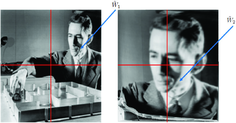
Figure 6: The Brenier optimal transport posterior matching scheme, zooming in on a point in a picture of Claude Shannon and his mouse. Left: Original picture of Shannon and his mouse from [48]. Right: optimally computed ‘zoomed’ in picture after application of $S_{y_{1}}$, where $y_{1}=1$ pertaining to the top right quadrant.

VII-C The Knothe-Rosenblatt Map for Higher Dimensional Problems

Assume ${\mathsf{W}}\subset\mathbb{R}^{d}$, and for any $w\in{\mathsf{W}}$, the $k$-th component of $w$ is denoted by $w[k]$, and likewise for $v$. We now consider the problem $\mathcal{L}(P_{W|Y=y},P_{W},c_{M})$ for $M\succ 0$ to find a map $S_{y}$ for which $S_{y}\#P_{W|Y=y}=P_{W}$ in Corollary IV.23. Assume that $M\equiv M_{\epsilon}$ is given by

$$M_{\epsilon}=\left[\begin{array}[]{c c c c}\alpha_{\epsilon}[1]&0&\ldots&0\\ 0&\alpha_{\epsilon}[2]&\ldots&0\\ \ldots&\ldots&\ldots&\ldots\\ 0&0&\ldots&\alpha_{\epsilon}[d]\end{array}\right]$$ (94)

Lemma VII.5

For ${\mathsf{W}}=[0,1]^{d}$, suppose

$$\lim_{\epsilon\to 0}\frac{\alpha_{\epsilon}[k+1]}{\alpha_{\epsilon}[k]}=0,\quad k=1,\ldots,d-1.$$ (95)

Then the optimal solution to $\mathcal{L}(P_{W|Y=y},P_{W},c_{M_{\epsilon}})$ converges as $\epsilon\to 0$ to a Knothe-Rosenblatt map. The limiting PM scheme becomes

$$w_{n+1}[1] =F_{W_{n}[1]|Y_{n}=y_{n}}(w_{n}[1])$$ (96a)

$$w_{n+1}[2] =F_{W_{n}[2]|Y_{n}=y_{n},W_{n+1}[1]=w_{n+1}[1]}(w_{n}[2])$$ (96b)

$$\ldots \ldots$$

Proof:

That the limit in (95) renders the Knothe-Rosenblatt map follows from [49]. That the Knothe-Rosenblatt map for the scenario where $P\equiv P_{W|Y=y}$ and $Q\equiv P_{W}$ is given by (96) is a direct application of [50]. ∎

In this case, $M_{\epsilon}$ has increasing weights $\alpha_{\epsilon}[k]$ in $k$. As such, preference is given more to certain axes of the message point as compared to the other. As such, the selection of the lopsided matrix $M_{\epsilon}$ in $\mathcal{L}(P_{W|Y=y},P_{W},M_{\epsilon})$ provides a rational design methodology to elicit PM schemes with unequal error protection [51, 52],

VII-D Multi-Antenna Communication as Multivariate Gaussian Channels

In this section we will take two routes to solve for the optimal mapping in an example case of a multi-antenna additive Gaussian noise with causal feedback. We consider the case where the covariance matrices of the noise and the capacity achieving inputs are not necessarily the identity matrix. We will find optimal couplings with respect to the symmetric Brenier cost and the Knothe-Rosenblatt cost, and show that in both cases, the schemes achieve capacity - although in very different ways. The former scheme will be shown to be the multi-dimensional analogue to the ‘innovations’ scheme by Schalkwijk and Kailath [3], while the latter can be interpreted from a ‘onion-peeling’ or ‘successive cancellation’ perspective [53].

Suppose we have a multi-antenna communication problem with feedback (Figure 7). As such, we model ${\mathsf{X}}={\mathsf{Y}}=\mathbb{R}^{d}$, where $d$ is the number of transmit antennas and also the number of receive antennas. Naturally, to develop a PM scheme where ${\mathsf{X}}={\mathsf{W}}$ satisfying Assumption III.1, it is desirable for $\Phi:{\mathsf{W}}\mapsto{\mathsf{X}}$ to be an invertible map for which $\dim({\mathsf{W}})=\dim({\mathsf{X}})$. As such, we model ${\mathsf{W}}=[0,1]^{d}$. We model the Gaussian noise as $Z_{i}\sim\mathscr{N}(0,\Sigma_{N})\in\mathbb{R}^{d}$ where $\Sigma_{N}$ is not necessarily diagonal. The received signal is given by $Y_{i}=X_{i}+Z_{i}$.

\begin{overpic}[width=303.53267pt]{fig7-MIMO-feedback-new2} \end{overpic}

Figure 7: Feedback communication over a Gaussian MIMO channel with feedback. $\dim({\mathsf{X}})>1$.

Under an average power constraint, the optimal input distribution is given by $P_{X}=\mathscr{N}(0,\Sigma_{X})$ for some $\Sigma_{X}$. Note that $P_{X_{1}|Y_{1}}=\mathscr{N}({\mathbb{E}}(X_{1}|Y_{1}),\Sigma_{X|Y})$. It can be directly shown [54, Prop 3.4.4] that ${\mathbb{E}}(X_{1}|Y_{1})=\Sigma_{X}\Sigma^{-1}_{Y}Y_{1}$ and $\Sigma_{X|Y}=\Sigma_{X}-\Sigma_{X}\Sigma^{-1}_{Y}\Sigma_{X}$. From Corollary IV.15, it follows that it is our desire to construct a PM-compatible map $\bar{S}_{y}\equiv\phi\circ S_{y}\phi^{-1}$ such that $\bar{S}_{y}\#P_{X_{1}|Y_{1}=y}=P_{X}^{*}$.

VII-D1 The Optimal Brenier Map for Higher Dimensional Problems

Here we consider finding a diffeomorphism $\bar{S}_{y}:\mathbb{R}^{d}\to\mathbb{R}^{d}$ that solves $\mathcal{L}(P_{X_{1}|Y_{1}=y},P_{X}^{*},I_{d\times d})$. [42, Theorem 3.4.1] provides the solution:

$$X_{n+1} = \bar{S}_{Y_{n}}(X_{n})=\alpha(X_{n}-\Sigma_{X}\Sigma^{-1}_{Y}Y_{n})$$ (97)

$$\alpha = \Sigma^{\frac{1}{2}}_{X}\left(\Sigma^{\frac{1}{2}}_{X}\Sigma_{X|Y}\Sigma^{\frac{1}{2}}_{X}\right)^{-\frac{1}{2}}\Sigma^{\frac{1}{2}}_{X}$$

Using MMSE estimation theory and Corollary IV.15, we can alternatively find the symmetric Brenier map by first positing that

$$X_{n+1}=\alpha(X_{n}-\beta Y_{n}).$$ (98)

with unknown $\alpha$ and $\beta$. $\beta=\Sigma_{X}\Sigma^{-1}_{Y}$ ensures that $X_{n+1}$ is independent of $Y_{n}$ (by joint Gaussianity and MMSE estimation), so we only need to find an invertible $\alpha$. Because all variables are jointly Gaussian, and since both sides of (98) have zero-means, we can simply operate on covariance matrices.

$$\Sigma_{X}=\alpha(\Sigma_{X|Y})\alpha^{T}=\alpha(\Sigma_{X}-\Sigma_{X}\Sigma^{-1}_{Y}\Sigma_{X})\alpha^{T}$$

It can be verified that this leads to the same linear algebra problem encountered in the OTT formulation solved by Olkin and Pukelsheim [55]:

$$\alpha=\Sigma^{\frac{1}{2}}_{X}\left(\Sigma^{\frac{1}{2}}_{X}\Sigma_{X|Y}\Sigma^{\frac{1}{2}}_{X}\right)^{-\frac{1}{2}}\Sigma^{\frac{1}{2}}_{X}.$$

As such, it follows that the optimal Brenier map is the $d$-dimensional Schalkwijk-Kailath scheme [3]. This $d$-dimensional scheme was also used to prove fundamental limits of control over noisy channels in [56].

Remark VII.6

It can be easily verified that the 1-dimensional case of [1, eqn. 22] that $X_{n+1}=\sqrt{1+\text{SNR}}(X_{n}-\frac{\text{SNR}}{1+\text{SNR}}Y_{n})$ is a natural derivation of the results (97) in higher dimension spaces.

VII-D2 The Optimal KR map and Successive Cancellation

Now consider the parameterized family $(M_{\epsilon})_{\epsilon>0}$ of positive definite matrices given by (94). Then these tend to the Knothe-Rosenblatt couplings, and analogous to Lemma VII.5, the optimal map in the two-dimensional Gaussian case is given by:

$$X_{n+1}[1] = \beta_{1}\left(X_{n}[1]-{\mathbb{E}}\left[X_{n}[1]|Y_{n}\right]\right)$$

$$X_{n+1}[2] = \beta_{2}\left(X_{n}[2]-{\mathbb{E}}\left[X_{n}[2]|Y_{n}\right]\right)+\beta_{3}X_{n+1}[1]$$

See [50] for the $\beta_{1},\beta_{2},\beta_{3}$ constants. This can be naturally extended for arbitrary $d>2$. Note that the essence of this scheme is successive cancellation [53] used to decode corner points in a multiple-access problem [34]: first decode the first dimension of $W$, followed by the second given knowledge of the first, etc. Here, we are using the chain rule to expand $I(W;Y)=I(W[1];Y)+I(W[2];Y|W[1])$. Thus, this has the potential to be applicable to unequal error protection scenarios where the first dimension of $W$ has more important information than the second.

VIII Discussion and Conclusion

In this paper, with the aid of optimal transport theory, we generalized the notion of posterior matching for message point feedback communication problems from the $(0,1)$ interval to $d$-dimensional Euclidean space. In addition, we developed notions of reliability and achievability from an almost-sure perspective and subsequently used classical probabilistic analysis methods to establish succinct necessary and sufficient conditions on when both reliability and achieving capacity occur: Birkhoff ergodicity of the $({\tilde{W}}_{n})_{n\geq 1}$ random process at the encoder. The applications included multi-antenna communications, and brain-computer interfaces.

Multiple theorems and lemmas established connections to modern applications including intrinsic methods for stability of the nonlinear filter in hidden Markov models and optimal transport theory. It may be fruitful to further cross-fertilize ideas between information theory and these areas. For instance, determining when the $({\tilde{W}}_{n})_{n\geq 1}$ random process is Birkhoff ergodic is a natural next question. In general, especially for continuous channels, this may be very challenging. Leveraging recent progress in optimal transport theory may enable the design of certain cost functions which guarantee the optimal $S_{y}^{*}$ results in ergodicity. Additionally, the surprising all-or-nothing nature between reliably communicating under PM schemes and the Birkhoff ergodicity of $({\tilde{W}}_{n})_{n\geq 1}$ could suggest new ways to transform questions about the ergodicity of a random process, into questions about appropriate channels under which they can be reliably communicated.

The use of optimal transport theory for posterior matching to construct a map to transform a sample from the posterior distribution on the message point $W$ to the prior distribution on $W$ is dual to optimal transport methods developed for Bayesian inference, where the objective is to construct a map that transforms a sample from the prior distribution on the latent variable into a sample from the posterior [57]. As such, this implies that for the same pair of posterior and prior, solving for a map for one problem simultaneously solves for the other (with taking an inverse). Recently developed convex optimization methods for Bayesian inference with optimal maps [58, 59, 60] thus may possibly leveraged for construction of maps within the context of posterior matching.

Future work could explore the Knothe-Rosenblatt optimal transport construction and its possible connection to “onion-peeling” successive cancellation decoding [53], as well as unequal error protection [52]. The fact that ergodicity is the if and only if condition for message point recovery and optimal convergence rates, suggests there might be further opportunities to use this type of mathematics to study optimization over stochastic dynamical systems problems in areas such as team decision theory (e.g. control over noisy channels [56, 61, 62]) and statistical physics [63].

Additionally, future work could focus on further developing the use of this framework for use in interacting systems of humans and machines beyond traditional brain-computer interfaces. For example, in the field of interactive reinforcement learning, some research has focus on systems in which a computer attempts to learn an optimal control policy from a human where sequential corrective action is being given by a human [64, 65, 66]. This generalization of the posterior matching scheme complements previous research [67, 12] into developing the necessary theory to maximize the efficiency of such systems.

References

• [1] O. Shayevitz and M. Feder, “Optimal feedback communication via posterior matching,” IEEE Transactions on Information Theory, vol. 57, no. 3, pp. 1186–1222, 2011.
• [2] M. Horstein, “Sequential transmission using noiseless feedback,” IEEE Transactions on Information Theory, vol. 9, no. 3, pp. 136–143, 1963.
• [3] J. Schalkwijk and T. Kailath, “A coding scheme for additive noise channels with feedback–I: No bandwidth constraint,” IEEE Transactions on Information Theory, vol. 12, no. 2, pp. 172–182, 1966.
• [4] S. Gorantla and T. P. Coleman, “Information-Theoretic Viewpoints on Optimal Causal Coding-Decoding Problems,” ArXiv e-prints, Feb. 2011.
• [5] O. Shayevitz, “Posterior matching variants and fixed-point elimination,” in Allerton Conference on Communication, Control, and Computing.   IEEE, 2009, pp. 935–939.
• [6] C. Omar, A. Akce, M. Johnson, T. Bretl, R. Ma, E. Maclin, M. McCormick, and T. P. Coleman, “A feedback information-theoretic approach to the design of brain–computer interfaces,” Intl. Journal of Human–Computer Interaction, vol. 27, no. 1, pp. 5–23, 2011.
• [7] J. Tantiongloc, D. A. Mesa, R. Ma, S. Kim, C. H. Alzate, J. J. Camacho, V. Manian, and T. P. Coleman, “An information and control framework for optimizing user-compliant human computer interfaces,” Proceedings of the IEEE, Feb 2017.
• [8] J. Schalkwijk, “A coding scheme for additive noise channels with feedback–II: Band-limited signals,” IEEE Transactions on Information Theory, vol. 12, no. 2, pp. 183–189, 1966.
• [9] T. M. Cover, “Enumerative source encoding,” IEEE Transactions on Information Theory, vol. 19, no. 1, pp. 73–77, 1973.
• [10] C. Omar, A. Akce, M. Johnson, T. Bretl, R. Ma, E. Maclin, M. McCormick, and T. P. Coleman, “A Feedback Information-Theoretic Approach to the Design of Brain-Computer Interfaces,” Int’l Journal on Human-Computer Interaction, January 2011, special issue on Current Trends in Brain-Computer Interface (BCI) Research.
• [11] A. Akce, M. Johnson, O. Dantsker, and T. Bretl, “A brain–machine interface to navigate a mobile robot in a planar workspace: enabling humans to fly simulated aircraft with eeg,” IEEE Transactions on Neural Systems and Rehabilitation Engineering, vol. 21, no. 2, pp. 306–318, 2013.
• [12] T. Tsiligkaridis, B. M. Sadler, and A. O. Hero, “Collaborative 20 questions for target localization,” IEEE Transactions on Information Theory, vol. 60, no. 4, pp. 2233–2252, 2014.
• [13] T. Tsiligkaridis, “Decentralized adaptive search using the noisy 20 questions framework in time-varying networks,” Signal Processing, 2017.
• [14] R. M. Castro and R. D. Nowak, “Minimax bounds for active learning,” IEEE Transactions on Information Theory, vol. 54, no. 5, pp. 2339–2353, 2008.
• [15] R. D. Nowak, “The geometry of generalized binary search,” IEEE Transactions on Information Theory, vol. 57, no. 12, pp. 7893–7906, 2011.
• [16] M. Naghshvar, T. Javidi, and M. Wigger, “Extrinsic jensen-shannon divergence: Applications to variable-length coding,” IEEE Transactions on Information Theory, vol. 61, no. 4, pp. 2148–2164, April 2015.
• [17] M. Naghshvar, T. Javidi et al., “Active sequential hypothesis testing,” The Annals of Statistics, vol. 41, no. 6, pp. 2703–2738, 2013.
• [18] Y. Kaspi, O. Shayevitz, and T. Javidi, “Searching with measurement dependent noise,” IEEE Transactions on Information Theory, vol. 64, no. 4, pp. 2690–2705, 2018.
• [19] S.-E. Chiu and T. Javidi, “Sequential measurement-dependent noisy search,” in Information Theory Workshop (ITW), 2016 IEEE.   IEEE, 2016, pp. 221–225.
• [20] A. Lalitha, N. Ronquillo, and T. Javidi, “Measurement dependent noisy search: The gaussian case,” in Information Theory (ISIT), 2017 IEEE International Symposium on.   IEEE, 2017, pp. 3090–3094.
• [21] J. H. Bae and A. Anastasopoulos, “A posterior matching scheme for finite-state channels with feedback,” in Information Theory Proceedings (ISIT), 2010 IEEE International Symposium on.   IEEE, 2010, pp. 2338–2342.
• [22] A. Anastasopoulos, “A sequential transmission scheme for unifilar finite-state channels with feedback based on posterior matching,” in Information Theory Proceedings (ISIT), 2012 IEEE International Symposium on.   IEEE, 2012, pp. 2914–2918.
• [23] J. Wu and A. Anastasopoulos, “Zero-rate achievability of posterior matching schemes for channels with memory,” in Information Theory (ISIT), 2016 IEEE International Symposium on.   IEEE, 2016, pp. 2384–2388.
• [24] A. Anastasopoulos and J. Wu, “Variable-length codes for channels with memory and feedback: error-exponent upper bounds,” arXiv preprint arXiv:1701.06678, 2017.
• [25] C. T. Li and A. El Gamal, “An efficient feedback coding scheme with low error probability for discrete memoryless channels,” IEEE Transactions on Information Theory, vol. 61, no. 6, pp. 2953–2963, June 2015.
• [26] O. Shayevitz and M. Feder, “A simple proof for the optimality of randomized posterior matching,” IEEE Transactions on Information Theory, vol. 62, no. 6, pp. 3410–3418, 2016.
• [27] R. Ma and T. P. Coleman, “Generalizing the posterior matching scheme to higher dimensions via optimal transportation,” in Allerton Conference on Communication, Control, and Computing.   IEEE, 2011, pp. 96–102.
• [28] R. Van Handel, “The stability of conditional Markov processes and Markov chains in random environments,” The Annals of Probability, vol. 37, no. 5, pp. 1876–1925, 2009.
• [29] P. Chigansky, R. Liptser, and R. Van Handel, “Intrinsic methods in filter stability,” Handbook of Nonlinear Filtering, 2009.
• [30] C. Villani, Optimal transport: old and new.   Springer Verlag, 2009.
• [31] D. Blackwell and D. Freedman, “The tail $\sigma$-field of a Markov chain and a theorem of Orey,” The Annals of Mathematical Statistics, 1964.
• [32] S. Verdú and T. S. Han, “A general formula for channel capacity,” IEEE Transactions on Information Theory, vol. 40, no. 4, pp. 1147–1157, 1994.
• [33] R. C. Bradley et al., “Basic properties of strong mixing conditions. a survey and some open questions,” Probability surveys, vol. 2, no. 2, pp. 107–144, 2005.
• [34] T. M. Cover and J. Thomas, Elements of Information Theory, 2nd ed.   Wiley-interscience, 2006.
• [35] W. Rudin, Real and complex analysis.   McGraw-Hill, 1987.
• [36] R. McEliece, The theory of information and coding.   Cambridge Univ Press, 2002.
• [37] Y. Kifer, Ergodic Theory of Random Transformations, 1986.
• [38] R. Van Handel, “When do nonlinear filters achieve maximal accuracy?” SIAM Journal on Control and Optimization, vol. 48, no. 5, pp. 3151–3168, 2009.
• [39] G. Monge, Mémoire sur la théorie des déblais et des remblais.   De l’Imprimerie Royale, 1781.
• [40] L. Kantorovich, “On mass transportation,” in Dokl. Akad. Nauk. SSSR, vol. 37, 1942, pp. 227–229.
• [41] C. Villani, Topics in optimal transportation.   American Mathematical Society, 2003.
• [42] S. Rachev and L. Rüschendorf, Mass transportation problems.   Springer Verlag, 1998, vol. 1.
• [43] T. Champion and L. De Pascale, “The Monge problem for strictly convex norms in $\mathbb{R}^{d}$,” Journal of the European Mathematical Society, vol. 12, no. 6, pp. 1355–1369, 2010.
• [44] R. V. Handel, Stochastic Calculus, Filtering, and Stochastic Control, 2007. [Online]. Available: http://www.princeton.edu/~rvan/acm217/ACM217.pdf
• [45] R. Gray, Entropy and information theory.   Springer-Verlag New York, Inc. New York, NY, USA, 1990.
• [46] L. Breiman, “Probability, classics in applied mathematics, vol. 7,” Society for Industrial and Applied Mathematics (SIAM), Pennsylvania, 1992.
• [47] A. Schlögl, F. Lee, H. Bischof, and G. Pfurtscheller, “Characterization of four-class motor imagery eeg data for the bci-competition 2005,” Journal of neural engineering, vol. 2, no. 4, p. L14, 2005.
• [48] Claude Shannon and experimental mouse maze constructed of relays demonstrated machine learning, 1952. [Online]. Available: http://www.computerhistory.org/collections/catalog/102630790
• [49] F. Santambrogio, A. Galichon, and G. Carlier, “From Knothe’s transport to Brenier’s map and a continuation method for optimal transport,” SIAM Journal on Mathematical Analysis, vol. 41, no. 6, p. 2554, 2010.
• [50] M. Rosenblatt, “Remarks on a multivariate transformation,” The Annals of Mathematical Statistics, vol. 23, no. 3, pp. 470–472, 1952.
• [51] S. Borade, B. Nakiboglu, and L. Zheng, “Unequal error protection: An information-theoretic perspective,” IEEE Transactions on Information Theory, vol. 55, no. 12, pp. 5511–5539, 2009.
• [52] B. Nakiboglu, S. K. Gorantla, L. Zheng, and T. P. Coleman, “Bit-wise unequal error protection for variable-length block codes with feedback,” IEEE Transactions on Information Theory, vol. 59, no. 3, pp. 1475–1504, 2013.
• [53] X. Zhang, J. Chen, S. B. Wicker, and T. Berger, “Successive coding in multiuser information theory,” IEEE Transactions on Information Theory, vol. 53, no. 6, pp. 2246–2254, 2007.
• [54] B. Hajek, An Exploration of Random Processes for Engineers, 2009. [Online]. Available: http://www.ifp.illinois.edu/~hajek/Papers/randomprocJan09.pdf
• [55] F. Olkin et al., “The distance between two random vectors with given dispersion matrices,” Linear Algebra and its Applications, vol. 48, pp. 257–263, 1982.
• [56] N. Elia, “When Bode meets Shannon: Control-oriented feedback communication schemes,” IEEE Transactions on Automatic Control, vol. 49, no. 5, pp. 1477–1488, 2004.
• [57] T. A. El Moselhy and Y. M. Marzouk, “Bayesian inference with optimal maps,” Journal of Computational Physics, vol. 231, no. 23, pp. 7815–7850, 2012.
• [58] S. Kim, C. J. Quinn, N. Kiyavash, and T. P. Coleman, “Dynamic and Succinct Statistical Analysis of Neuroscience Data,” Proceeding of IEEE, vol. 102, pp. 683–698, 2014.
• [59] D. A. Mesa, S. Kim, and T. P. Coleman, “A scalable framework to transform samples from one continuous distribution to another,” in ISIT, 2015.
• [60] D. A. Mesa, J. Tantiongloc, M. Mendoza, and T. P. Coleman, “A distributed framework for the construction of transport maps,” Neural Computation, forthcoming.
• [61] E. Ardestanizadeh and M. Franceschetti, “Control-theoretic approach to communication with feedback,” IEEE Transactions on Automatic Control, vol. 57, no. 10, pp. 2576–2587, 2012.
• [62] A. A. Kulkarni and T. P. Coleman, “An optimizer’s approach to stochastic control problems with nonclassical information structures,” IEEE Transactions on Automatic Control, vol. 60, no. 4, pp. 937–949, 2015.
• [63] S. K. Mitter and N. J. Newton, “Information and entropy flow in the Kalman–Bucy filter,” Journal of Statistical Physics, vol. 118, no. 1-2, pp. 145–176, 2005.
• [64] W. B. Knox and P. Stone, “Tamer: Training an agent manually via evaluative reinforcement,” in Development and Learning, 2008. ICDL 2008. 7th IEEE International Conference on.   IEEE, 2008, pp. 292–297.
• [65] N. A. Vien, W. Ertel, and T. C. Chung, “Learning via human feedback in continuous state and action spaces,” Applied intelligence, vol. 39, no. 2, pp. 267–278, 2013.
• [66] C. Meriçli, M. Veloso, and H. L. Akin, “Complementary humanoid behavior shaping using corrective demonstration,” in Humanoid Robots (Humanoids), 2010 10th IEEE-RAS International Conference on.   IEEE, 2010, pp. 334–339.
• [67] R. M. Castro, C. Kalish, R. Nowak, R. Qian, T. Rogers, and X. Zhu, “Human active learning,” in Advances in neural information processing systems, 2009, pp. 241–248.