On the Capabilities and Limitations of [DK: Multi-hop] Reasoning
for Natural Language Understanding

On the Possibilities and Limitations of Multi-hop Reasoning
Under Linguistic Imperfections

Abstract

Systems for language understanding have become remarkably strong at overcoming linguistic imperfections in tasks involving phrase matching or simple reasoning. Yet, their accuracy drops dramatically as the number of reasoning steps increases. We present the first formal framework to study such empirical observations. It allows one to quantify the amount and effect of ambiguity, redundancy, incompleteness, and inaccuracy that the use of language introduces when representing a hidden conceptual space. The idea is to consider two interrelated spaces: a conceptual meaning space that is unambiguous and complete but hidden, and a linguistic space that captures a noisy grounding of the meaning space in the words of a language—the level at which all systems, whether neural or symbolic, operate. Applying this framework to a special class of multi-hop reasoning, namely the connectivity problem in graphs of relationships between concepts, we derive rigorous intuitions and impossibility results even under this simplified setting. For instance, if a query requires a moderately large (logarithmic) number of hops in the meaning graph, no reasoning system operating over a noisy graph grounded in language is likely to correctly answer it. This highlights a fundamental barrier that extends to a broader class of reasoning problems and systems, and suggests an alternative path forward: focusing on aligning the two spaces via richer representations, before investing in reasoning with many hops.

1 Introduction

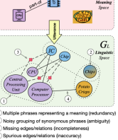
Figure 1: The interface between meanings and words capturing linguistic imperfections: each meaning (top) can be uttered in many ways as words (bottom), and the same word can have multiple meanings.

Reasoning can be viewed as the process of combining facts and beliefs, in order to infer new conclusions Johnson-Laird (1980). While there is a rich literature on reasoning, there is limited understanding of it in the context of natural language, particularly in the presence of linguistic noise. There remains a substantial gap between the strong empirical performance and little theoretical understanding of models for common language tasks, such as question answering, reading comprehension, and textual entailment. We focus on multi-hop or multi-step reasoning over text, where one must take multiple steps and combine multiple pieces of information to arrive at the correct conclusion. Remarkably, the accuracy of even the best multi-hop models is empirically known to drop drastically as the number of required hops increases Yang et al. (2018); Mihaylov et al. (2018). This is generally viewed as a consequence of linguistic imperfections, such as those illustrated in Figure 1.

We introduce a novel formalism that quantifies these imperfections and makes it possible to theoretically analyze a subclass of multi-hop reasoning algorithms. Our results provide formal support for existing empirical intuitions about the limitations of reasoning with inherently noisy language. Importantly, our formalism can be applied to both neural as well as symbolic systems, as long as they operate on natural language input.

The formalism consists of (A) an abstract model of linguistic knowledge, and (B) a reasoning model. The abstract model is built around the notion of two spaces (see Figure 1): a hidden meaning space of unambiguous concepts and an associated linguistic space capturing their imperfect grounding in words. The reasoning model captures the ability to infer a property of interest in the meaning space (e.g., the relationship between two concepts) while observing only its imperfect representation in the linguistic space.

The interaction between the meaning space and the linguistic space can be seen as simulating and quantifying the symbol-grounding problem Harnad (1990), a key difficulty in operating over language that arises when one tries to accurately map words into their underlying meaning representation. Practitioners often address this challenge by enriching their representations; for example by mapping textual information to Wikipedia entries Mihalcea and Csomai (2007); Ratinov et al. (2011), grounding text to executable rules via semantic parsing Reddy et al. (2017), or incorporating contexts into representations Peters et al. (2018); Devlin et al. (2019). Our results indicate that advances in higher fidelity representations are key to making progress in multi-hop reasoning.

There are many flavors of multi-hop reasoning, such as finding a particular path of labeled edges through the linguistic space (e.g., textual multi-hop reasoning) or performing discrete operations over a set of such paths (e.g., semantic parsing). In this first study, we explore a common primitive shared by various tasks, namely, the connectivity problem: Can we determine whether there is a path of length $k$ between a pair of nodes in the meaning graph, while observing only its noisy grounding as the linguistic graph? This simplification clarifies the exposition and analysis; we expect similar impossibility results, as the ones we derive, to hold for a broader class of tasks that rely on connectivity.

We note that even this simplified setting by itself captures interesting cases. Consider the task of inferring the Is-a relationship, by reasoning over a noisy taxonomic graph extracted from language. For instance, is it true that “a chip” Is-a “a nutrient”? When these elements cannot be directly looked up in a curated resource such as WordNet Miller (1995) (e.g., in low-resource languages, for scientific terms, etc.), recognizing the Is-a relationship between “a chip” and “a nutrient” would require finding a path in the linguistic space connecting “a chip” to “a nutrient”, while addressing the associated word-sense issues. Is-a edges would need to be extracted from text, resulting in potentially missing and/or extra edges. This corresponds precisely to the linguistic inaccuracies modeled and quantified in our framework.

Contributions.

This is the first mathematical study of the challenges and limitations of reasoning algorithms in the presence of the symbol-meaning mapping difficulty. Our main contributions are:

1. Formal Framework. We establish a novel, linguistically motivated formal framework for analyzing the problem of reasoning about the ground truth (the meaning space) while operating over its noisy linguistic representation. This allows one to derive rigorous intuitions about what various classes of reasoning algorithms can and cannot achieve. 2. Impossibility Results. We study in detail the connectivity reasoning problem, focusing on the interplay between linguistic noise (redundancy, ambiguity, incompleteness, and inaccuracy) and the distance (inference steps, or hops) between two concepts in the meaning space. We prove that under low noise, reliable connectivity reasoning is indeed possible up to a few hops (Theorem 1). In contrast, even a moderate increase in the noise level makes it provably impossible to assess the connectivity of concepts if they are a logarithmic distance apart in terms of the meaning graph nodes (Theorems 2 and 3). This helps us understand empirical observations of “semantic drift” in systems, causing a substantial performance drop beyond 2-3 hops Fried et al. (2015); Jansen (2016). We discuss practical lessons from our findings, such as focusing on richer representations and higher-quality abstractions to reduce the number of hops.

3. Empirical Illustration. While our main contribution is theoretical, we use the experiments to illustrate the implications of our results in a controlled setting. Specifically, we apply the framework to a subset of a real-world knowledge-base, FB15k237 Toutanova and Chen (2015), treated as the meaning graph, illustrating how key parameters of our analytical model influence the possibility (or impossibility) of accurately solving the connectivity problem.

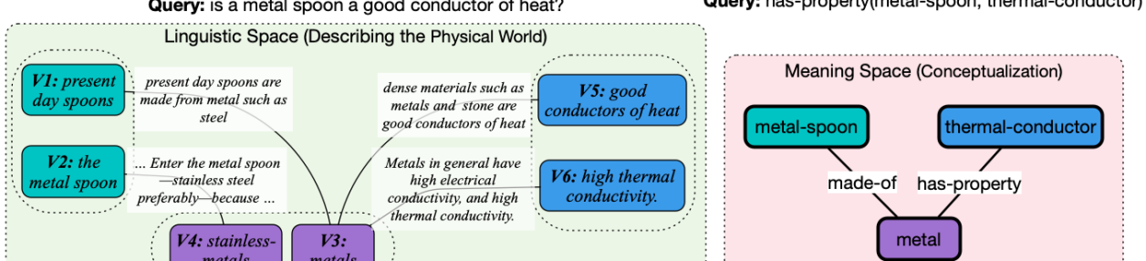
Figure 2: The meaning graph (right) captures a clean and unique (canonical) representation of concepts and facts, while the linguistic graph (left) contains a noisy, incomplete, and redundant representation of the same knowledge. Shown here are samples of meaning graph nodes and the corresponding linguistic graph nodes for answering the question: Is a metal spoon a good conductor of heat?. Relationships in the linguistic graph are here indirectly represented via sentences.

2 Overview of the Formalism

(A) Linguistically-inspired abstract model.

We propose an abstract model of linguistic knowledge built around the notion of two spaces (see Figures 1 and 2). The meaning space refers to the internal conceptualization in human mind, where we assume the information is free of noise and uncertainty. In contrast to human thinking that happens in this noise-free space, human expression of thought via the utterence of language introduces many imperfections, and happens in the linguistic space. This linguistic space is often redundant (e.g., multiple words such as “CPU” and “computer processor” express the same meaning), ambiguous (e.g., a word like “chips” could refer to multiple meanings ), incomplete (e.g., common-sense relations never expressed in text), and inaccurate (e.g., incorrect facts written down in text). Importantly, the noisy linguistic space—with its redundancy, ambiguity, incompleteness, and inaccuracy—is what a machine reasoning algorithm operates in.

(B) Reasoning model.

For the purposes of this work, we define reasoning as the ability to infer the existence or absence of a property of interest in the meaning space, by only observing its imperfect representation in the linguistic space. Specifically, we focus on properties that can be captured by graphs, namely the meaning graph which connects concepts via semantic relationships, and the (noisy) linguistic graph which connects words via language. Nodes in the linguistic graph may represent words in various ways, such as using symbols Miller (1995), fixed vectors Mikolov et al. (2013), or even words in context as captured by contextual vectors Peters et al. (2018); Devlin et al. (2019).

The target property in the meaning graph characterizes the reasoning task. E.g., relation extraction corresponds to determining the relationship between two meaning graph nodes, by observing their grounding in text as linguistic graph nodes. Word sense disambiguation (WSD) corresponds to identifying a meaning graph node given a word (a node in the linguistic graph) and its surrounding context. Question-answering may ask for a linguistic node that has a desired semantic relationship (when mapped to the meaning space) to another given node (e.g., what is the capital of X?).

2.1 Example

Figure 2 illustrates a reasoning setting that includes edge semantics. Most humans understand that V1:“present day spoons” and V2:“the metal spoons” are equivalent nodes (have the same meaning) for the purposes of the query, “is a metal spoon a good conductor of heat?”. However, a machine must infer this. In the linguistic space (left), the semantics of the connections between nodes are expressed through natural language sentences, which also provide a context for the nodes. For example, edges in the meaning graph (right) directly express the semantic relation has-property(metal, thermal-conductor), while a machine, operating on language, may struggle to infer this from reading Internet text expressed in various ways, e.g., “dense materials such as [V3:]metals and stones are [V5:]good conductors of heat”.

To ground this in existing efforts, consider multi-hop reasoning for QA systems Khashabi et al. (2016); Jansen et al. (2018). Here the reasoning task is to connect local information, via multiple local “hops”, in order to arrive at a conclusion. In the meaning graph, one can trace a path of locally connected nodes to verify the correctness of a query; for example, the query has-property(metal-spoon, thermal-conductor) can be verified by tracing a sequence of nodes in Fig. 2. Thus, answering some queries can be cast as inferring the existence of a path connecting two nodes. While doing so on the meaning graph is straightforward, reliably doing so on the noisy linguistic graph is not. Intuitively, each local “hop” introduces additional noise, allowing reliable inference to be performed only when it does not require too many steps in the underlying meaning graph. To study this issue, our approach quantifies the effect of noise accumulation for long-range reasoning.

3 Related Work

AI literature contains a variety of formalisms for automated reasoning, including reasoning with logical representations McCarthy (1963), semantic networks Quillan (1966), Bayesian networks Pearl (1988), etc. For our analysis, we use a graphical formalism since it provides a useful modeling tool and is a commonly used abstraction for representing items and relations between them.

One major challenge in reasoning with natural language tasks is grounding free-form text to a higher-level meaning. Example proposals to deal with this challenge include semantic parsing Steedman and Baldridge (2011), linking to a knowledge base Mihalcea and Csomai (2007), and mapping to semantic frames Punyakanok et al. (2004). These methods can be viewed as approximate solutions to the symbol-grounding problem Harnad (1990); Taddeo and Floridi (2005) — the challenge of mapping symbols to a representation that reflect their accurate meaning. Our formalism is an effort to better understand the fundamental difficulties that this problem poses.

Several efforts focus on reasoning with disambiguated inputs, such as using executable formulas Reddy et al. (2017); Angeli and Manning (2014) and chaining relations to infer new relations Socher et al. (2013). Our analysis covers any algorithm for inferring patterns that can be represented in a graphical form, e.g., chaining local information, often referred to as multi-hop reasoning Jansen et al. (2016); Lin et al. (2018). For example, Jansen et al. Jansen et al. (2017) propose a structured multi-hop reasoning approach by aggregating sentential information from multiple KBs. They demonstrate improvements with few hops and degradation when aggregating more than 2-3 sentences. Our theoretical findings align well with such observations and further quantify them.

4 The Meaning-Language Interface

We formalize our conceptual and linguistic notions of knowledge spaces as undirected graphs:

• The meaning space, $M$, is a conceptual hidden space where all the facts are accurate and complete, without ambiguity. We focus on the knowledge in this space that can be represented as an undirected graph, $G_{M}$($V_{M}$, $E_{M}$). This knowledge is hidden, and representative of the information that exists within human minds.

• The linguistic space, $L$, is the space of knowledge represented in natural language for machine consumption (written sentences, curated knowledge-bases, etc.). We assume access to a graph $G_{L}$($V_{L}$, $E_{L}$) in this space that is a noisy approximation of $G_{M}$.

The two spaces interact: when we read a sentence, we are reading from the linguistic space and interpreting it in the meaning space. When writing out our thoughts, we symbolize our thought process, by moving them from meaning space to the linguistic space. Fig.1 provides a high-level view of this interaction.

A reasoning system operates in the linguistic space and is unaware of the exact structure and information encoded in $G_{M}$. How well it performs depends on the local connectivity of $G_{M}$ and the level of noise in $G_{L}$, which is discussed next.

4.1 Meaning-to-Language mapping

Let $\text{$\mathcal{O}$}:V_{M}\rightarrow 2^{V_{L}}$ denote an oracle function that captures the set of nodes in $G_{L}$ that each (hidden) node in $G_{M}$ should ideally map to in a noise-free setting. This represents multiple ways in which a single meaning can be equivalently represented in language. When $w\in\text{$\mathcal{O}$}(m)$, i.e., $w$ is one of the words the oracle maps a meaning $m$ to, we write $\text{$\mathcal{O}$}^{-1}(w)=m$ to denote the reverse mapping. For example, if CHIP represents a node in the meaning graph for the common snack food, then $\mathcal{O}$(CHIP) = {“potato chips”, “crisps”, …}.

Ideally, if two nodes $m_{1}$ and $m_{2}$ in $V_{M}$ have an edge in $G_{M}$, we would want an edge between every pair of nodes in $\text{$\mathcal{O}$}(m_{1})\times\text{$\mathcal{O}$}(m_{2})$ in $G_{L}$. The actual graph $G_{L}$ (discussed next) will be a noisy approximation of this ideal case.

4.2 Generative Model of Linguistic Graphs

Linguistic graphs in our framework are constructed via a generative process. Starting with $G_{M}$, we sample $G_{L}\leftarrow\mathsf{ALG}(G_{M})$ using a stochastic process described in Alg.1. Informally, the algorithm simulates the process of transforming conceptual information into linguistic utterances (web-pages, conversations, knowledge bases, etc.). This construction captures a few key properties of linguistic representation of meaning via 3 control parameters: replication factor $\lambda$, edge retention probability $p_{+}$, and spurious edge creation probability $p_{-}$.

Input: Meaning graph $G_{M}$($V_{M}$, $E_{M}$), discrete distribution $r(\lambda)$, edge retention prob. $p_{+}$, edge creation prob. $p_{-}$

Output: Linguistic graph $G_{L}$($V_{L}$, $E_{L}$)

foreach $v\in\text{$V_{M}$}$ do

       sample $k\sim r(\lambda)$

       construct a collection of new nodes $U$ s.t. $|U|=k$

       $\text{$V_{L}$}\leftarrow\text{$V_{L}$}\cup U$,    $\mathcal{O}$$(v)\leftarrow U$

      

foreach $(m_{1},m_{2})\in(\text{$V_{M}$}\times\text{$V_{M}$}),m_{1}\neq m_{2}$ do

       $W_{1}\leftarrow\text{$\mathcal{O}$}(m_{1})$, $W_{2}\leftarrow\text{$\mathcal{O}$}(m_{2})$

       foreach $e\in W_{1}\times W_{2}$ do

             if $(m_{1},m_{2})\in\text{$E_{M}$}$ then

                   with probability $p_{+}$: $\text{$E_{L}$}\leftarrow\text{$E_{L}$}\cup\{e\}$

            else

                   with probability $p_{-}$: $\text{$E_{L}$}\leftarrow\text{$E_{L}$}\cup\{e\}$

            

      

Algorithm 1 Generative, stochastic construction of a linguistic graph $G_{L}$ given a meaning graph $G_{M}$.

Each node in $G_{M}$ is mapped to multiple linguistic nodes (the exact number drawn from a distribution $r(\lambda)$, parameterized by $\lambda$), which models redundancy in $G_{L}$. Incompleteness of knowledge is modeled by not having all edges of $G_{M}$ be retained in $G_{L}$ (controlled by $p_{+}$). Further, $G_{L}$ contains spurious edges that do not correspond to any edge in $G_{M}$, representing inaccuracy (controlled by $p_{-}$). The extreme case of noise-free construction of $G_{L}$ corresponds to having $r(\lambda)$ be concentrated at $1$, $p_{+}=1$, and $p_{-}=0$.

4.3 Noisy Similarity Metric

Additionally, we include linguistic similarity based edges to model ambiguity, i.e., a single word mapping to multiple meanings. Specifically, we view ambiguity as treating (or confusing) two distinct linguistic nodes for the same word as identical even when they correspond to different meaning nodes (e.g., confusing a “bat” node for animals with a “bat” node for sports).

Similarity metrics are typically used to judge the equivalence of words, with or without context. Let $\rho:V_{L}\times V_{L}\rightarrow\{0,1\}$ be such a metric, where $\rho(w,w^{\prime})=1$ for $w,w^{\prime}\in V_{L}$ denotes the equivalence of these two nodes in $G_{L}$. We define $\rho$ to be a noisy version of the true node similarity as determined by the oracle $\mathcal{O}$:

$$\rho(w,w^{\prime})\triangleq \begin{cases}1-\text{Bern}(\varepsilon_{+})&\text{if\ }\text{$\mathcal{O}$}^{-1}(w)=\text{$\mathcal{O}$}^{-1}(w^{\prime})\\ \text{Bern}(\varepsilon_{-})&\text{otherwise}\end{cases},\vspace{-0.1cm}$$

where $\varepsilon_{+},\varepsilon_{-}\in(0,1)$ are the noise parameters of $\rho$, both typically close to zero, and Bern$(p)$ denotes the Bernoulli distribution with parameter $p$.

Intuitively, $\rho$ is a perturbed version of true similarity (as defined by $\mathcal{O}$), with small random noise (parameterized with $\varepsilon_{+}$ and $\varepsilon_{-}$). With a high probability $1-\varepsilon_{+/-}$, $\rho$ returns the correct similarity decision as determined by the oracle (i.e., whether two words have the same meaning). The extreme case of $\varepsilon_{+}=\varepsilon_{-}=0$ models the perfect similarity metric. In practice, even the best similarity systems are noisy, captured here with $\varepsilon_{+/-}>0$.

We assume reasoning algorithms have access to $G_{L}$ and $\rho$, and that they use the following procedure to verify the existence of a direct connection between two nodes:

function NodePairConnectivity($w,w^{\prime}$)

     return $(w,w^{\prime})\in E_{L}$   or   $\rho(w,w^{\prime})=1$

Several corner cases result in uninteresting meaning or linguistic graphs. We focus on a regime of “non-trivial” cases where $G_{M}$ is neither overly-connected nor overly-sparse, there is non-zero noise ($p_{-},\varepsilon_{-},\varepsilon_{+}>0$) and incomplete information ($p_{+}<1$), and noisy content does not dominate actual information (e.g., $p_{-}\ll p_{+}$). Henceforth, we consider only such “non-trivial” instances.

Throughout, we will also assume that the replication factor (i.e., the number of linguistic nodes corresponding to each meaning node) is a constant, i.e., $r$ is such that $\mathbb{P}\left[|U|=\lambda\right]=1$.

5 Hypothesis Testing Setup: Reasoning About Meaning via Words

While a reasoning engine only sees the linguistic graph $G_{L}$, it must make inferences about the latent meaning graph $G_{M}$. Given a pair of nodes $\mathbf{v_{L}}:=\{w,w^{\prime}\}\subset V_{L}$, the reasoning algorithm must then predict properties about the corresponding nodes $\mathbf{v_{M}}=\{m,m^{\prime}\}=\{\text{$\mathcal{O}$}^{-1}(w),\text{$\mathcal{O}$}^{-1}(w^{\prime})\}$.

We use a hypothesis testing setup to assess the likelihood of two disjoint hypotheses defined over $G_{M}$, denoted $H^{\leavevmode\hbox to6.65pt{\vbox to6.65pt{\text{[drawing]}}}}_{M}(\mathbf{v_{M}})$ and $H^{\leavevmode\hbox to6.65pt{\vbox to6.65pt{\text{[drawing]}}}}_{M}(\mathbf{v_{M}})$ (e.g., whether $\mathbf{v_{M}}$ are connected in $G_{M}$ or not). Given observations $X_{L}(\mathbf{v_{L}})$ about linguistic nodes (e.g., whether $\mathbf{v_{L}}$ are connected in $G_{L}$), we define the goal of a reasoning algorithm as inferring which of the two hypotheses about $G_{M}$ is more likely to have resulted in these observations, under the sampling process (Alg.1). That is, we are interested in:

$$\underset{h\in\{H^{\leavevmode\hbox to6.65pt{\vbox to6.65pt{\text{[drawing]}}}}_{M}(\mathbf{v_{M}}),H^{\leavevmode\hbox to6.65pt{\vbox to6.65pt{\text{[drawing]}}}}_{M}(\mathbf{v_{M}})\}}{\text{argmax}}\mathbb{P}^{(h)}\left[X_{L}(\mathbf{v_{L}})\right]\vspace{-0.03cm}$$ (1)

where $\mathbb{P}^{(h)}\left[x\right]$ denotes the probability of an event $x$ in the sample space induced by Alg.1, when (hidden) $G_{M}$ satisfies hypothesis $h$. Defn. 6 in the Appendix formalizes this.

Since we start with two disjoint hypotheses on $G_{M}$, the resulting probability spaces are generally different, making it plausible to identify the correct hypothesis with high confidence. However, with sufficient noise in the sampling process, it can be difficult for an algorithm based on the linguistic graph to distinguish the two resulting probability spaces (corresponding to the two hypotheses), depending on observations $X_{L}(\mathbf{v_{L}})$ used by the algorithm and the parameters of the sampling process. For example, the distance between linguistic nodes can often be an insufficient indicator for distinguishing these two hypotheses. We will explore these two contrasting behaviors in the next section.

Not all observations are equally effective in distinguishing $h_{1}$ from $h_{2}$. We say $X_{L}(\mathbf{v_{L}})$ $\gamma$-separates them if:

$$\mathbb{P}^{(h_{1})}\left[X_{L}(\mathbf{v_{L}})\right]-\mathbb{P}^{(h_{2})}\left[X_{L}(\mathbf{v_{L}})\right]\,\geq\,\gamma.$$ (2)

(formal definition in Appendix, Defn. 7) We can view $\gamma$ as the gap between the likelihoods of $X_{L}(\mathbf{v_{L}})$ having originated from a meaning graph satisfying $h_{1}$ vs. one satisfying $h_{2}$. When $\gamma=1$, $X_{L}(\mathbf{v_{L}})$ is a perfect discriminator for $h_{1}$ and $h_{2}$. In general, any positive $\gamma$ bounded away from $1$ yields a valuable observation, and a reasoning algorithm:

function Separator$\_{X_{L}}$($\text{{$G_{L}$}},\mathbf{v_{L}}=\{w,w^{\prime}\}$)

     if $X_{L}(\mathbf{v_{L}})=1$ then return $h_{1}$ else return $h_{2}$

Importantly, this algorithm does not compute the probabilities in Eqs. (1) and  (2). Rather, it works with a particular instantiation $G_{L}$. We refer to such an algorithm $\mathcal{A}$ as $\gamma$-accurate for $h_{1}$ and $h_{2}$ if, under the sampling choices of Alg.1, it outputs the ‘correct’ hypothesis with probability at least $\gamma$; that is, for both $i\in\{1,2\}$: $\mathbb{P}^{(h_{i})}\left[\mathcal{A}\text{\ outputs\ }h_{i}\right]\geq\gamma$. This happens when $X_{L}$ $\gamma$-separates $h_{1}$ and $h_{2}$ (cf. Appendix, Prop. 8). The rest of the work will explore when one can obtain a $\gamma$-accurate algorithm, using $\gamma$-separation of the underlying observation as an analysis tool.

6 Main Results (Informal)

Having formalized a model of the meaning-language interface above, we now present our main findings. The results in this section are intentionally stated in a somewhat informal manner for ease of exposition and to help convey the main messages clearly. Formal mathematical statements and supporting proofs are deferred to the Appendix.

One simple but often effective approach for reasoning is to focus on connectivity (as described in Fig. 2). Specifically, we consider reasoning chains as valid if they correspond to a short path in the meaning space, and invalid if they correspond to disconnected nodes. Mathematically, this translates into the $d$-connectivity reasoning problem, defined as follows: Given access to a linguistic graph $G_{L}$ and two nodes $w,w^{\prime}$ in it, let $m=\text{$\mathcal{O}$}^{-1}(w)$ and $m^{\prime}=\text{$\mathcal{O}$}^{-1}(w^{\prime})$ denote the corresponding nodes in the (hidden) meaning graph $G_{M}$. While observing only $G_{L}$, can we distinguish between two hypotheses about $G_{M}$, namely, $m,m^{\prime}$ have a path of length $d$ in $G_{M}$, vs. $m,m^{\prime}$ are disconnected? Distinguishing between these two hypotheses, namely $h_{1}=m\overset{d}{\leftrightsquigarrow}m^{\prime}$ and $h_{2}=m\overset{}{\cancel{\leftrightsquigarrow}}m^{\prime}$, is the problem we are interested in solving.

The answer clearly depends on how faithfully $G_{L}$ reflects $G_{M}$. In the (unrealistic) noise-free case of $G_{L}$ = $G_{M}$, this problem is trivially solvable by computing the shortest path between $w$ and $w^{\prime}$ in $G_{L}$. More realistically, the higher the noise level is in Alg.1 and NodePairSimilarity, the harder it will be for any algorithm operating on $G_{L}$ to confidently infer a property of $G_{M}$.

In other words, the redundancy, ambiguity, incompleteness and inaccuracy of language discussed earlier directly impact the capability and limitations of algorithms that perform connectivity reasoning. Our goal is to quantify this intuition using the parameters $p_{+},p_{-},\lambda,\varepsilon_{+},\varepsilon_{-}$ of our generative model, and derive possibility and impossibility results.

A simple connectivity testing algorithm.

The first set of results assume the following algorithm: given $w,w^{\prime}$ with a desired distance $d$ in $G_{M}$, it checks whether $w,w^{\prime}$ have a path of length at most $\tilde{d}$, which is a function of $d$ and the replication factor $\lambda$. If yes, it declares the corresponding meaning nodes $m,m^{\prime}$ in $G_{M}$ have a path of length $d$; otherwise it declares them disconnected.

Let $a\oplus b$ denote $a+b-ab$, and $\text{$\mathcal{B}$}(d)$ denote the maximum number of nodes within distance $d$ of any node in $G_{M}$. The following result shows that even the simple algorithm above guarantees accurate reasoning (specifically, it correctly infers connectivity in $G_{M}$ while only observing $G_{L}$) for limited noise and small $d$ (i.e., few hops):

Theorem 1 (Possibility Result; Informal).

If $p_{-},\varepsilon_{-},d,$ and $\gamma$ are small enough such that $(p_{-}\oplus\varepsilon_{-})\cdot\text{$\mathcal{B}$}^{2}(d)<\frac{1}{2e\lambda^{2}n}$, then there exists a $\gamma\in[0,1]$ that increases with $p_{+},\lambda$ and decreases with $\varepsilon_{+}$, such that the simple connectivity testing algorithm with $\tilde{d}=\lambda\cdot d+\lambda-1$ correctly solves the $d$-connectivity problem with probability at least $\gamma$.

Here, the probability is over the sampling choices of Alg. 1 when constructing $G_{L}$, and the function NodePairConnectivity for determining node similarity in $G_{L}$.

On the other hand, when there is more noise and $d$ becomes even moderately large—specifically, logarithmic in the number of nodes in $G_{M}$—then this simple algorithm no longer works even for small values of desired accuracy $\gamma$:

Theorem 2 (Impossibility Result #1; Informal).

If $p_{-}$ and $\varepsilon_{-}$ are large enough such that $p_{-}\oplus\varepsilon_{-}\geq\frac{c}{\lambda n}$ and $d\in\Omega(\log n)$ where $n$ is the number of nodes in $G_{M}$, then the simple connectivity algorithm with $\tilde{d}=\lambda d$ cannot solve the $d$-connectivity problem correctly with probability $\gamma$ for any $\gamma>0$.

This result exposes an inherent limitation to multi-hop reasoning: even for small values of noise, the diameter of $G_{L}$ can quickly become very small, namely, logarithmic in $n$ (similar to the small-world phenomenon observed by Milgram Milgram (1967) in other contexts), at which point the above impossibility result kicks in. Our result affirms that if NLP reasoning algorithms are not designed carefully, such macro behaviors will necessarily become bottlenecks, even for relatively simple tasks such as detecting connectivity.

The above result is for the simple connectivity algorithm. One can imagine other ways to determine connectivity in $G_{M}$, such as by analyzing the degree distribution of $G_{L}$, looking at its clustering structure, etc. Our third finding extends the impossibility result to this general setting, showing that if the noise level is increased a little more (by a logarithmic factor), then no algorithm can infer connectivity in $G_{M}$ by observing only $G_{L}$:

Theorem 3 (Impossibility Result #2; Informal).

If $p_{-}$ and $\varepsilon_{-}$ are large enough such that $p_{-}\oplus\varepsilon_{-}>\frac{c\log n}{\lambda n}$ and $d>\log n$ where $n$ is the number of nodes in $G_{M}$, then any algorithm cannot correctly solve the $d$-connectivity problem correctly with probability $\gamma$ for any $\gamma>0$.

This reveals a fundamental limitation, that we may only be able to infer interesting properties of $G_{M}$ within small, logarithmic sized neighborhoods. We leave the formal counterparts of these results (Theorems 11, 12, and 13, resp.) to Appendix B, and focus next on a small scale empirical validation to complement our analytical findings.

7 Empirical Validation

Our formal analysis thus far offers worst-case bounds for two regions in a fairly large spectrum of noisy sampling parameters for the linguistic space, namely, when $p_{-}\oplus\varepsilon_{-}$ and $d$ are either both small (Theorem 1), or both large (Theorems 2 and 3).

This section complements our theoretical findings in two ways: (a) by grounding the formalism empirically into a real-world knowledge graph, (b) by quantifying the impact of sampling parameters on the connectivity algorithm. We use $\varepsilon_{-}=0$ for the experiments, but the effect turns out to be identical to using $\varepsilon_{-}>0$ for appropriate adjustments of $p_{-}$ and $p_{+}$ (see Remark 9 in the Appendix).

We consider FB15k237 Toutanova and Chen (2015), a set of $\langle$head, relation, target$\rangle$ triples from FreeBase Bollacker et al. (2008). For scalability, we use the movies domain subset (relations /film/*), with 2855 entity nodes and 4682 relation edges. We treat this as the meaning graph $G_{M}$ and sample a linguistic graph $G_{L}$ (via Alg.1) to simulate the observed graph derived from text.

We sample $G_{L}$ for various values of $p_{-}$ and plot the resulting distances in $G_{L}$ and $G_{M}$ in Fig. 3, as follows. For every value of $p_{-}$ ($y$-axis), we sample pairs of points in $G_{M}$ that are separated by distance $d$ ($x$-axis). For these pairs of points, we compute the average distance between the corresponding linguistic nodes (in sampled $G_{L}$), and plot that in the heat map using color shades.

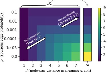
Figure 3: Colors in the figure depict the average distance between node-pairs in $G_{L}$, for each true distance $d$ (x-axis) in $G_{M}$, as the noise parameter $p_{-}$ (y-axis) is varied. The goal is to distinguish squares in the column for a particular $d$ with the corresponding squares in the right-most column, which corresponds to node-pairs being disconnected. This is easy in the bottom-left regime and becomes progressively harder as we move upward (more noise) or rightward (higher distance in $G_{M}$). ($\varepsilon_{+}=0.7,\lambda=3$)

We make two observations from this simulation. First, for lower values of $p_{-}$, disconnected nodes in $G_{M}$ (rightmost column) are clearly distinguishable from meaning nodes with short paths (small $d$) as predicted by Theorem 11, but harder to distinguish from nodes at large distances (large $d$). Second, and in contrast, for higher values of $p_{-}$, almost every pair of linguistic nodes is connected with a very short path (dark color), making it impossible for a distance-based reasoning algorithm to confidently assess $d$-connectivity in $G_{M}$. This simulation also confirms our finding in Theorem 12: any graph with $p_{-}\geq 1/\lambda n$ (which is $\sim 0.0001$ here) cannot distinguish disconnected meaning nodes from nodes with paths of short (logarithmic) length (top rows).

8 Implications and Practical Lessons

Our analysis is motivated by empirical observations of “semantic drift” of reasoning algorithms, as the number of hops is increased. For example, Fried et al. Fried et al. (2015) show modest benefits up to 2-3 hops, and then decreasing performance; Jansen et al. Jansen et al. (2018) make similar observations in graphs built out of larger structures such as sentences, where the performance drops off around 2 hops. This pattern has interestingly been observed under a variety of representations, including word-level input, graphs, and traversal methods. A natural question is whether the field might be hitting a fundamental limit on multi-hop information aggregation. Our “impossibility” results are reaffirmations of the empirical intuition in the field. This means that multi-hop inference (and any algorithm that can be cast in that form), as we’ve been approaching it, is exceptionally unlikely to breach the few-hop barrier predicted in our analysis.

There are at least two practical lessons: First, our results suggest that ongoing efforts on “very long” multi-hop reasoning, especially without a careful understanding of the limitations, are unlikely to succeed, unless some fundamental building blocks are altered. Second, this observation suggests that practitioners must focus on richer representations that allow reasoning with only a “few” hops. This, in part, requires higher-fidelity abstraction and grounding mechanisms. It also points to alternatives, such as offline KB completion/expansion mechanisms, which indirectly reduce the number of steps needed at inference time.

Our formal results quantify how different linguistic imperfection parameters affect multi-hop reasoning differently. This provides an informed design choice for which noise parameter to try to control when creating a new representation.

9 Conclusion

This work is the first attempt to develop a formal framework for understanding the behavior of complex natural language reasoning in the presence of linguistic noise. The importance of this work is two-fold. First, it proposes a novel graph-theoretic paradigm for studying reasoning, inspired by the symbol-meaning problem in the presence of redundancy, ambiguity, incompleteness, and inaccuracy of language. Second, it shows how to use this framework to analyze a class of reasoning algorithms. We expect our findings, as well as those from future extensions to other classes of reasoning algorithms, to have important implications on how we study problems in language comprehension.

To focus the main text on key findings and intuitions, we abstract away many technical details. Here instead we go into the formal proofs with the necessary mathematical rigor. We start with our requisite definitions (§A), followed by formal statements of our three results (§B), and their proofs (§C, §D, §E). We conclude the supplementary material with additional empirical results (§F).

Appendix A Definitions: Reasoning Problems, Hypothesis Testing Setup, and $\gamma$-Separation

Notation.

Throughout, we follow the standard notation for asymptotic comparison of functions: $O(.)$, $o(.)$, $\Theta(.)$, $\Omega(.),$ and $\omega(.)$ Cormen et al. (2009). $X\sim f(\theta)$ denotes a random variable $X$ distributed according to probability distribution $f(\theta)$, paramterized by $\theta$. $\text{Bern}(p)$ and $\text{Bin}(n,p)$ denote the Bernoulli and Binomial distributions, respectively. Given random variables $X\sim\text{Bern}(p)$ and $Y\sim\text{Bern}(q)$, their disjunction $X\vee Y$ is distributed as $\text{Bern}(p\oplus q)$, where $p\oplus q\triangleq 1-(1-p)(1-q)=p+q-pq$. We make extensive use of this notation.

Let $\mathrm{dist}(u,v)$ be the distance between nodes $u$ and $v$ in $G$. A simple path (henceforth referred to as just a path) is a sequence of adjacent nodes that does not have repeating nodes. Let $u\overset{d}{\leftrightsquigarrow}v$ denote the existence of a path of length $d$ between $u$ and $v$. Similarly, $u\overset{}{\cancel{\leftrightsquigarrow}}v$ denotes $u$ and $v$ are disconnected. The notion of $d$-neighborhood is useful when analyzing local properties of graphs:

Definition 4.

For a graph $G=(V,E)$, $w\in V$, and $d\in\mathbb{N}$, the $d$-neighborhood of $w$ is $\{v\mid\mathrm{dist}(w,v)\leq d\}$, i.e., the ‘ball’ of radius $d$ around $w$. $\text{$\mathcal{B}$}(w,d)$ denotes the number of nodes in this $d$-neighborhood, and $\text{$\mathcal{B}$}(d)=\max_{w\in V}\text{$\mathcal{B}$}(w,d)$.

For the rest of this section we formally the key concepts used in the main text, as well as those necessary for our formal proofs.

Definition 5 (Nontrivial Graph Instances).

A pair ($\text{{$G_{M}$}},\text{{$G_{L}$}}$) of a meaning graph and a linguistic graph created from it is non-trivial if its generation process satisfies the following: 1. non-zero noise, i.e., $p_{-},\varepsilon_{-},\varepsilon_{+}>0$; 2. incomplete information, i.e., $p_{+}<1$; 3. noise content does not dominate the actual information, i.e., $p_{-}\ll p_{+}$, $\varepsilon_{+}<0.5$, and $p_{+}>0.5$; 4. $G_{M}$ is not overly-connected, i.e., $\text{$\mathcal{B}$}(d)\in o(n)$, where $n$ is the number of nodes in $G_{M}$; 5. $G_{M}$ is not overly-sparse, i.e., $|E_{G_{M}}|\in\omega(1)$.

While the reasoning engine only sees the linguistic graph $G_{L}$, it must make inferences about the potential latent meaning graph. Given a pair of nodes $\mathbf{v_{L}}:=\{w,w^{\prime}\}\subset V_{L}$ in the linguistic graph, the reasoning algorithm must then predict properties about the corresponding nodes $\mathbf{v_{M}}=\{m,m^{\prime}\}=\{\text{$\mathcal{O}$}^{-1}(w),\text{$\mathcal{O}$}^{-1}(w^{\prime})\}$ in the meaning graph.

We use a hypothesis testing setup to assess the likelihood of two disjoint hypotheses defined over $G_{M}$: $H^{\leavevmode\hbox to6.65pt{\vbox to6.65pt{\text{[drawing]}}}}_{M}(\mathbf{v_{M}})$ and $H^{\leavevmode\hbox to6.65pt{\vbox to6.65pt{\text{[drawing]}}}}_{M}(\mathbf{v_{M}})$. Given observations $X_{L}(\mathbf{v_{L}})$ about linguistic nodes, the goal of a reasoning algorithm here is to identify which of the two hypotheses about $G_{M}$ is more likely to have resulted in these observations, under the sampling process of Algorithm 1. That is, we are interested in:

$$\underset{h\in\{H^{\leavevmode\hbox to6.65pt{\vbox to6.65pt{\text{[drawing]}}}}_{M}(\mathbf{v_{M}}),H^{\leavevmode\hbox to6.65pt{\vbox to6.65pt{\text{[drawing]}}}}_{M}(\mathbf{v_{M}})\}}{\text{argmax}}\mathbb{P}^{(h)}\left[X_{L}(\mathbf{v_{L}})\right]$$ (3)

where $\mathbb{P}^{(h)}\left[x\right]$ denotes the probability of an event $x$ in the sample space induced by Algorithm 1, when the (hidden) meaning graph $G_{M}$ satisfies hypothesis $h$. Formally:

Definition 6 (Reasoning Problem).

The input for an instance $\mathcal{P}$ of the reasoning problem is a collection of parameters that characterize how a linguistic graph $G_{L}$ is generated from a (latent) meaning graph $G_{M}$, two hypotheses $H^{\leavevmode\hbox to6.65pt{\vbox to6.65pt{\text{[drawing]}}}}_{M}(\mathbf{v_{M}}),H^{\leavevmode\hbox to6.65pt{\vbox to6.65pt{\text{[drawing]}}}}_{M}(\mathbf{v_{M}})$ about $G_{M}$, and available observations $X_{L}(\mathbf{v_{L}})$ in $G_{L}$. The reasoning problem, $\mathcal{P}(p_{+}$, $p_{-}$, $\varepsilon_{+}$, $\varepsilon_{-}$, $\text{$\mathcal{B}$}(d)$, n, $\lambda$, $H^{\leavevmode\hbox to6.65pt{\vbox to6.65pt{\text{[drawing]}}}}_{M}(\mathbf{v_{M}})$, $H^{\leavevmode\hbox to6.65pt{\vbox to6.65pt{\text{[drawing]}}}}_{M}(\mathbf{v_{M}})$, $X_{L}(\mathbf{v_{L}}))$, is to map the input to the hypothesis $h$ as per Eq. (1).

Since we start with two disjoint hypotheses on $G_{M}$, the resulting probability spaces are generally different, making it plausible to identify the correct hypothesis with high confidence. On the other hand, with sufficient noise in the sampling process, it can also become difficult for an algorithm to distinguish the two resulting probability spaces (corresponding to the two hypotheses), especially depending on the observations $X_{L}(\mathbf{v_{L}})$ used by the algorithm and the parameters of the sampling process. For example, the distance between linguistic nodes can often be an insufficient indicator for distinguishing these two hypotheses. We will explore these two contrasting reasoning behaviors in the next section.

We use “separation” to measure how effective is an observation $X_{L}$ in distinguishing between the two hypotheses:

Definition 7 ($\gamma$-Separation).

For $\gamma\in[0,1]$ and a reasoning problem instance $\mathcal{P}$ with two hypotheses $h_{1}=H^{\leavevmode\hbox to6.65pt{\vbox to6.65pt{\text{[drawing]}}}}_{M}(\mathbf{v_{M}})$ and $h_{2}=H^{\leavevmode\hbox to6.65pt{\vbox to6.65pt{\text{[drawing]}}}}_{M}(\mathbf{v_{M}})$, we say an observation $X_{L}(\mathbf{v_{L}})$ in the linguistic space $\gamma$-separates $h_{1}$ from $h_{2}$ if: $$\mathbb{P}^{(h_{1})}\left[X_{L}(\mathbf{v_{L}})\right]-\mathbb{P}^{(h_{2})}\left[X_{L}(\mathbf{v_{L}})\right]\,\geq\,\gamma.$$ We can view $\gamma$ as the gap between the likelihoods of the observation $X_{L}(\mathbf{v_{L}})$ having originated from a meaning graph satisfying hypothesis $h_{1}$ vs. one satisfying hypothesis $h_{2}$. When $\gamma=1$, $X_{L}(\mathbf{v_{L}})$ is a perfect discriminator for distinguishing $h_{1}$ and $h_{2}$. In general, any positive $\gamma$ bounded away from $1$ yields a valuable observation.

Given an observation $X_{L}$ that $\gamma$-separates $h_{1}$ and $h_{2}$, there is a simple algorithm that distinguishes $h_{1}$ from $h_{2}$:

function Separator${}_{X_{L}}$($\text{{$G_{L}$}},\mathbf{v_{L}}=\{w,w^{\prime}\}$)

     if $X_{L}(\mathbf{v_{L}})=1$ then return $h_{1}$ else return $h_{2}$

Importantly, this algorithm does not compute the probabilities in Definition 7. Rather, it works with a particular instantiation $G_{L}$ of the linguistic graph. We refer to such an algorithm $\mathcal{A}$ as $\gamma$-accurate for $h_{1}$ and $h_{2}$ if, under the sampling choices of Algorithm 1, it outputs the ‘correct’ hypothesis with probability at least $\gamma$; that is, for both $i\in\{1,2\}$: $\mathbb{P}^{(h_{i})}\left[\mathcal{A}\text{\ outputs\ }h_{i}\right]\geq\gamma.$

Proposition 8.

If observation $X_{L}$ $\gamma$-separates $h_{1}$ and $h_{2}$, then algorithm Separator${}_{X_{L}}$ is $\gamma$-accurate for $h_{1}$ and $h_{2}$.

Proof.

Let $\mathcal{A}$ denote Separator${}_{X_{L}}$ for brevity. Combining $\gamma$-separation of $X_{L}$ with how $\mathcal{A}$ operates, we obtain:

$$\mathbb{P}^{(h_{1})}\left[\mathcal{A}\text{\ outputs\ }h_{1}\right]-\mathbb{P}^{(h_{2})}\left[\mathcal{A}\text{\ outputs\ }h_{1}\right] \geq\gamma$$

$$\Rightarrow\mathbb{P}^{(h_{1})}\left[\mathcal{A}\text{\ outputs\ }h_{1}\right]+\mathbb{P}^{(h_{2})}\left[\mathcal{A}\text{\ outputs\ }h_{2}\right] \geq 1+\gamma$$

Since each term on the left is bounded above by $1$, each of them must also be at least $\gamma$, as desired. ∎

The rest of the work will explore when one can obtain a $\gamma$-accurate algorithm, using $\gamma$-separation of the underlying observation as an analysis tool.

The following observation allows a simplification of the proofs, without loss of any generality.

Remark 9.

Since our procedure doesn’t treat similarity edges and meaning-to-symbol noise edges differently, we can ‘fold’ $\varepsilon_{-}$ into $p_{-}$ and $p_{+}$ (by increasing edge probabilities). More generally, the results are identical whether one uses $p_{+},p_{-},\varepsilon_{-}$ or $p^{\prime}_{+},p^{\prime}_{-},\varepsilon^{\prime}_{-}$, as long as: $$\begin{cases}p_{+}\oplus\varepsilon_{-}=p^{\prime}_{+}\oplus\varepsilon^{\prime}_{-}\\ p_{-}\oplus\varepsilon_{-}=p^{\prime}_{-}\oplus\varepsilon^{\prime}_{-}\end{cases}$$ For any $p_{+}$ and $\varepsilon_{-}$, we can find a $p^{\prime}_{+}$ such that $\varepsilon^{\prime}_{-}$ = 0. Thus, w.l.o.g., in the following analysis we derive results only using $p_{+}$ and $p_{-}$ (i.e. assume $\varepsilon^{\prime}_{-}$ = 0). Note that we expand these terms to $p_{+}\oplus\varepsilon_{-}$ and $p_{-}\oplus\varepsilon_{-}$ respectively in the final results.

Appendix B Main Results (Formal)

This section presents a more formal version of our results. As discussed below, the formal theorems are best stated using the notions of hypothesis testing, observations on linguistic graphs $G_{L}$, and $\gamma$-separation of two hypotheses about $G_{M}$ using these observations on $G_{L}$.

B.1 Connectivity Reasoning Algorithm

For nodes $m,m^{\prime}$ in $G_{M}$, we refer to distinguishing the following two hypotheses as the $d$-connectivity reasoning problem and find that even these two extreme worlds can be difficult to separate:

$$h_{1}=m\overset{d}{\leftrightsquigarrow}m^{\prime}\text{,\ \ and\ \ }\;h_{2}=m\overset{}{\cancel{\leftrightsquigarrow}}m^{\prime}$$

For reasoning algorithms, a natural test is the connectivity of linguistic nodes in $G_{L}$ via the NodePairConnectivity function. Specifically, checking whether there is a path of length $\leq\tilde{d}$ between $w,w^{\prime}$:

$$X^{\tilde{d}}_{L}(w,w^{\prime})=\;w\overset{\leq\tilde{d}}{\leftrightsquigarrow}w^{\prime}$$

Existing multi-hop reasoning models Khot et al. (2017) use similar approaches to identify valid reasoning chains.

The corresponding connectivity algorithm is Separator$\_{X^{\tilde{d}}_{L}}$, which we would like to be $\gamma$-accurate for $h_{1}$ and $h_{2}$. Next, we derive bounds on $\gamma$ for these specific hypotheses and observations $X_{L}(\mathbf{v_{L}})$. While the space of possible hypotheses and observations is large, the above natural and simple choices still allow us to derive valuable intuitions.

B.1.1 Possibility of Accurate Connectivity Reasoning

We begin by defining the following accuracy threshold, $\gamma^{*}$, as a function of the parameters for sampling a linguistic graph:

Definition 10.

Given $n,d\in\mathbb{N}$ and linguistic graph sampling parameters $p_{+},\varepsilon_{+},\lambda$, define $\gamma^{*}(n,d,p_{+},\varepsilon_{+},\varepsilon_{-},\lambda)$ as $$\left(1-\left(1-(p_{+}\oplus\varepsilon_{-})\right)^{\lambda^{2}}\right)^{d}\cdot\left(1-2e^{3}\varepsilon_{+}^{\lambda/2}\right)^{d+1}-2en(\lambda\text{$\mathcal{B}$}(d))^{2}p_{-}.$$ This expression, although complex-looking, behaves in a natural way. E.g., the accuracy threshold $\gamma^{*}$ increases (higher accuracy) as $p_{+}$ increases (higher edge retention) or $\varepsilon_{+}$ decreases (fewer dropped connections between replicas). Similarly, as $\lambda$ increases (higher replication), the impact of the noise on edges between node clusters or $d$ decreases (shorter paths), again increasing the accuracy threshold.

Theorem 11 (formal statement of Theorem 1).

Let $p_{+},p_{-},\lambda$ be the parameters of Alg.1 on a meaning graph with $n$ nodes. Let $\varepsilon_{+},\varepsilon_{-}$ be the parameters of NodePairConnectivity. Let $d\in\mathbb{N}$ and $\tilde{d}=\lambda\cdot d+\lambda-1$. If $${\color[rgb]{0,0,0}{(p_{-}\oplus\varepsilon_{-})}}\cdot\text{$\mathcal{B}$}^{2}(d)<\frac{1}{{\color[rgb]{0,0,0}}\lambda^{2}n},$$ and $\gamma=\max\{0,\gamma^{*}(n,d,p_{+},\varepsilon_{+},\varepsilon_{-},\lambda)\}$, then algorithm Separator$\_{X^{\tilde{d}}_{L}}$ is $\gamma$-accurate for $d$-connectivity problem.

B.2 Limits of Connectivity-Based Algorithms

We show that as the distance $d$ between two meaning nodes increases, it becomes difficult to make any inference about their connectivity by assessing connectivity of the corresponding linguistic-graph nodes. Specifically, if $d$ is at least logarithmic in the number of meaning nodes, then, even with small noise, the algorithm will see all node-pairs as being within distance $d$, making informative inference unlikely.

Theorem 12 (formal statement of Theorem 2).

Let $c>1$ be a constant and $p_{-},\lambda$ be parameters of the sampling process in Alg.1 on a meaning graph $G_{M}$ with $n$ nodes. Let $\varepsilon_{-}$ be a parameter of NodePairConnectivity. Let $d\in\mathbb{N}$ and $\tilde{d}=\lambda d$. If $$\vspace{-0.01cm}{\color[rgb]{0,0,0}{p_{-}\oplus\varepsilon_{-}}}\geq\frac{c}{\lambda n}\ \ \ \text{and}\ \ \ d\in\Omega(\log n),\vspace{-0.01cm}$$ then the connectivity algorithm Separator$\_{X^{\tilde{d}}_{L}}$ almost-surely infers any node-pair in $G_{M}$ as connected, and is thus not $\gamma$-accurate for any $\gamma>0$ for the $d$-connectivity problem.

Note that preconditions of Theorems 11 and 12 are disjoint, that is, both results don’t apply simultaneously. Since $\text{$\mathcal{B}$}(.)\geq 1$ and $\lambda\geq 1$, Theorem 11 requires ${\color[rgb]{0,0,0}{p_{-}\oplus\varepsilon_{-}}}\leq{\color[rgb]{0,0,0}{\frac{1}{{\color[rgb]{0,0,0}}\lambda^{2}n}<\frac{1}{\lambda^{2}n}}}$, whereas Theorem 12 applies when ${\color[rgb]{0,0,0}{p_{-}\oplus\varepsilon_{-}}}\geq\frac{c}{\lambda n}>\frac{1}{\lambda^{2}n}$.

B.3 Limits of General Algorithms

We now extend the result to an algorithm agnostic setting, where no assumption is made on the choice of the Separator algorithm or $X_{L}(\mathbf{v_{L}})$. For instance, $X_{L}(\mathbf{v_{L}})$ could make use of the entire degree distribution of $G_{L}$, compute the number of disjoint paths between various linguistic nodes, cluster nodes, etc. The analysis uses spectral properties of graphs to quantify local information.

Theorem 13 (formal statement of Theorem 3).

Let $c>0$ be a constant and $p_{-},\lambda$ be parameters of the sampling process in Alg.1 on a meaning graph $G_{M}$ with $n$ nodes. Let $\varepsilon_{-}$ be a parameter of NodePairConnectivity. Let $d\in\mathbb{N}$. If $${\color[rgb]{0,0,0}{p_{-}\oplus\varepsilon_{-}}}>\frac{c\log n}{\lambda n}\ \ \ \text{and}\ \ \ d>\log n,$$ then there exists $n_{0}\in\mathbb{N}$ s.t. for all $n\geq n_{0}$, no algorithm can distinguish, with a high probability, between two nodes in $G_{M}$ having a $d$-path vs. being disconnected, and is thus not $\gamma$-accurate for any $\gamma>0$ for the $d$-connectivity problem.

This reveals a fundamental limitation: under noisy conditions, our ability to infer interesting phenomena in the meaning space is limited to a small, logarithmic neighborhood.

Appendix C Proofs: Possibility of Accurate Connectivity Reasoning

In this section we provide the proofs of the additional lemmas necessary for proving the intermediate results. First we introduce a few useful lemmas, and then move on to the proof of Theorem 11.

We introduce the following lemmas which will be used in connectivity analysis of the clusters of the nodes $\text{$\mathcal{O}$}(m)$.

Lemma 14 (Connectivity of a random graph Gilbert (1959)).

Let $P_{n}$ denote the probability of the event that a random undirected graph $\mathsf{G(n,p)}$ ($p>0.5$) is connected. This probability can be lower-bounded as following: $$P_{n}\geq 1-\left[q^{n-1}\left\{(1+q^{(n-2)/2})^{n-1}-q^{(n-2)(n-1)/2}\right\}+q^{n/2}\left\{(1+q^{(n-2)/2})^{n-1}-1\right\}\right],$$ where $q=1-p$.

See Gilbert Gilbert (1959) for a proof of this lemma. Since $q\in(0,1)$, this implies that $P_{n}\rightarrow 1$ as $n$ increases. The following lemma provides a simpler version of the above probability:

Corollary 15 (Connectivity of a random graph Gilbert (1959)).

The random-graph connectivity probability $P_{n}$ (Lemma 14) can be lower-bounded as following: $$P_{n}\geq 1-2e^{3}q^{n/2}$$

Proof.

We use the following inequality:

$$(1+\frac{3}{n})^{n}\leq e^{3}$$

Given that $q\leq 0.5,n\geq 1$, one can verify that $q^{(n-2)/2}\leq 3/n$. Combining this with the above inequality gives us, $(1+q^{{n-2}/2})^{n-1}\leq e^{3}$.

With this, we bound the two terms within the two terms of the target inequality:

$$\begin{cases}(1+q^{(n-2)/2})^{n-1}-q^{(n-2)(n-1)/2}\leq e^{3}\\ (1+q^{(n-2)/2})^{n-1}-1\leq e^{3}\end{cases}$$

$$\left[q^{n-1}\left\{(1+q^{(n-2)/2})^{n-1}-q^{(n-2)(n-1)/2}\right\}+q^{n/2}\left\{(1+q^{(n-2)/2})^{n-1}-1\right\}\right]\leq e^{3}q^{n-1}+e^{3}q^{n/2}\leq 2e^{3}q^{n/2}$$

which concludes the proof.

∎

We show a lower-bound on the probability of $w$ and $w^{\prime}$ being connected given the connectivity of their counterpart nodes in the meaning graph. Notice that the choice of $\tilde{d}=(d+1)(\lambda-1)+d=\lambda\cdot d+\lambda-1$ is calculated as follows: The type of paths from $w$ to $w^{\prime}$, we consider for the proof, has at most $\lambda-1$ edges within the nodes corresponding to one single meaning node, and $d$ edges in between. This lemma will be used in the proof of Theorem 11:

Lemma 16 (Lower bound).

$\mathbb{P}\left[w\overset{\tilde{d}}{\leftrightsquigarrow}w^{\prime}|m\overset{d}{\leftrightsquigarrow}m^{\prime}\right]\geq\left(1-2e^{3}\varepsilon_{+}^{\lambda/2}\right)^{d+1}\cdot\left(1-(1-p_{+})^{\lambda^{2}}\right)^{d}$.

Proof.

We know that $m$ and $m^{\prime}$ are connected through some intermediate nodes $m_{1},m_{2},\cdots,m_{\ell}$ ($\ell<d$). We show a lower-bound on having a path in the linguistic graph between $w$ and $w^{\prime}$, through clusters of nodes $\text{$\mathcal{O}$}(m_{1}),\text{$\mathcal{O}$}(m_{2}),\cdots,\text{$\mathcal{O}$}(m_{\ell})$. We decompose this into two events:

$$\begin{cases}e_{1}[v]&\text{For a given meaning node }v\text{ its cluster in the linguistic graph, }\text{$\mathcal{O}$}(v)\text{ is connected. }\\ e_{2}[v,u]&\text{For any two connected nodes }(u,v)\text{ in the meaning graph, there is at least an edge}\\ &\text{connecting their clusters }\text{$\mathcal{O}$}(u),\text{$\mathcal{O}$}(v)\text{ in the linguistic graph.}\end{cases}$$

The desired probability can then be refactored as:

$$\mathbb{P}\left[w\overset{\tilde{d}}{\leftrightsquigarrow}w^{\prime}|m\overset{d}{\leftrightsquigarrow}m^{\prime}\right] \geq\mathbb{P}\left[\left(\bigcap_{v\in\{w,m_{1},\dots,m_{\ell},w^{\prime}\}}e_{1}[v]\right)\cap\left(\bigcap_{(v,u)\in\{(w,m_{1}),\dots,(m_{\ell},w^{\prime})\}}e_{2}[v,u]\right)\right]$$

$$\geq\mathbb{P}\left[e_{1}\right]^{d+1}\cdot\mathbb{P}\left[e_{2}\right]^{d}.$$

We split the two probabilities and identify lower bounds for each. Based on Corollary 15, $\mathbb{P}\left[e_{1}\right]\geq 1-2e^{3}\varepsilon_{+}^{\lambda/2}$, and as a result $\mathbb{P}\left[e_{1}\right]^{d+1}\geq\left(1-2e^{3}\varepsilon_{+}^{\lambda/2}\right)^{d+1}$. The probability of connectivity between pair of clusters is $\mathbb{P}\left[e_{2}\right]=1-(1-p_{+})^{\lambda^{2}}$. Thus, similarly, $\mathbb{P}\left[e_{2}\right]^{d}\geq\left(1-(1-p_{+})^{\lambda^{2}}\right)^{d}$. Combining these two, we obtain:

$$\mathbb{P}\left[w\overset{\tilde{d}}{\leftrightsquigarrow}w^{\prime}|m\overset{d}{\leftrightsquigarrow}m^{\prime}\right]\geq\left(1-2e^{3}\varepsilon_{+}^{\lambda/2}\right)^{d+1}\cdot\left(1-(1-p_{+})^{\lambda^{2}}\right)^{d}$$ (4)

∎

The connectivity analysis of $G_{L}$ can be challenging since the graph is a non-homogeneous combination of positive and negative edges. For the sake of simplifying the probabilistic arguments, given linguistic graph $G_{L}$, we introduce a non-unique simple graph $\tilde{G}_{L}$ as follows.

Definition 17.

Consider a special partitioning of $V_{G}$ such that the $d$-neighbourhoods of $w$ and $w^{\prime}$ form two of the partitions and the rest of the nodes are arbitrarily partitioned in a way that the diameter of each component does not exceed $\tilde{d}$. • The set of nodes $V_{\tilde{G}_{L}}$ of $\tilde{G}_{L}$ corresponds to the aforementioned partitions. • There is an edge $(u,v)\in E_{\tilde{G}_{L}}$ if and only if at least one node-pair from the partitions of $V_{G}$ corresponding to $u$ and $v$, respectively, is connected in $E_{G_{L}}$.

In the following lemma we give an upper-bound on the connectivity of neighboring nodes in $\tilde{G}_{L}$:

Lemma 18.

When $G_{L}$ is drawn at random, the probability that an edge connects two arbitrary nodes in $\tilde{G}_{L}$ is at most $(\lambda\text{$\mathcal{B}$}(d))^{2}p_{-}$.

Proof.

Recall that a pair of nodes from $\tilde{G}_{L}$, say $(u,v)$, are connected when at least one pair of nodes from corresponding partitions in $G_{L}$ are connected. Each $d$-neighbourhood in the meaning graph has at most $\text{$\mathcal{B}$}(d)$ nodes. It implies that each partition in $\tilde{G}_{L}$ has at most $\lambda\text{$\mathcal{B}$}(d)$ nodes. Therefore, between each pair of partitions, there are at most $(\lambda\text{$\mathcal{B}$}(d))^{2}$ possible edges. By union bound, the probability of at least one edge being present between two partitions is at most $(\lambda\text{$\mathcal{B}$}(d))^{2}p_{-}$. ∎

Let $v_{w},v_{w^{\prime}}\in V_{\tilde{G}_{L}}$ be the nodes corresponding to the components containing $w$ and $w^{\prime}$ respectively. The following lemma establishes a relation between connectivity of $w,w^{\prime}\in V_{G_{L}}$ and the connectivity of $v_{s},v_{w^{\prime}}\in V_{\tilde{G}_{L}}$:

Lemma 19.

$\mathbb{P}\left[w\overset{\tilde{d}}{\leftrightsquigarrow}w^{\prime}|m\overset{}{\cancel{\leftrightsquigarrow}}m^{\prime}\right]\leq\mathbb{P}\left[\text{There is a path from $v_{s}$ to $v_{w^{\prime}}$ in $\tilde{G}_{L}$ with length }\tilde{d}\right]$.

Proof.

Let $L$ and $R$ be the events in the left hand side and right hand side respectively. Also for a permutation of nodes in $G_{L}$, say $p$, let $F_{p}$ denote the event that all the edges of $p$ are present, i.e., $L=\cup F_{p}$. Similarly, for a permutation of nodes in $\tilde{G}_{L}$, say $q$, let $H_{q}$ denote the event that all the edges of $q$ are present. Notice that $F_{p}\subseteq H_{q}$ for $q\subseteq p$, because if all the edges of $p$ are present the edges of $q$ will be present. Thus,

$$L=\bigcup_{p}F_{p}\subseteq\bigcup_{p}H_{p\cap E_{\tilde{G}_{L}}}=\bigcup_{q}H_{q}=R.$$

This implies that $\mathbb{P}\left[L\right]\leq\mathbb{P}\left[R\right]$. ∎

Lemma 20 (Upper bound).

If $(\lambda\text{$\mathcal{B}$}(d))^{2}p_{-}\leq\frac{1}{2en}$, then $\mathbb{P}\left[w\overset{\leq\tilde{d}}{\leftrightsquigarrow}w^{\prime}\mid m\overset{}{\cancel{\leftrightsquigarrow}}m^{\prime}\right]\leq 2en(\lambda\text{$\mathcal{B}$}(d))^{2}p_{-}.$

Proof.

To identify the upper bound on $\mathbb{P}\left[w\overset{\leq\tilde{d}}{\leftrightsquigarrow}w^{\prime}|m\overset{}{\cancel{\leftrightsquigarrow}}m^{\prime}\right]$, recall the definition of $\tilde{G}_{L}$, given an instance of $G_{L}$ (as outlined in Lemma 18 and Lemma 19, for $\tilde{p}=(\lambda\text{$\mathcal{B}$}(d))^{2}p_{-}$). Lemma 19 relates the connectivity of $w$ and $w^{\prime}$ to a connectivity event in $\tilde{G}_{L}$, i.e., $\mathbb{P}\left[w\overset{\leq\tilde{d}}{\leftrightsquigarrow}w^{\prime}\mid m\overset{}{\cancel{\leftrightsquigarrow}}m^{\prime}\right]\leq\mathbb{P}\left[\text{there is a path from $v_{s}$ to $v_{w^{\prime}}$ in $\tilde{G}_{L}$ with length }\tilde{d}\right]$, where $v_{s},v_{w^{\prime}}\in V_{\tilde{G}_{L}}$ are the nodes corresponding to the components containing $w$ and $w^{\prime}$ respectively. Equivalently, in the following, we prove that the event $\text{dist}(v_{s},v_{w^{\prime}})\leq\tilde{d}$ happens with a small probability:

$$\mathbb{P}\left[w\overset{\leq\tilde{d}}{\leftrightsquigarrow}w^{\prime}\right]=\mathbb{P}\left[\bigvee_{\ell=1,\cdots,\tilde{d}}w\overset{\ell}{\leftrightsquigarrow}w^{\prime}\right]\leq\sum_{\ell\leq\tilde{d}}{n\choose\ell}\tilde{p}^{\ell}\leq\sum_{\ell\leq\tilde{d}}(\frac{en}{\ell})^{\ell}\tilde{p}^{\ell}$$

$$\leq\sum_{\ell\leq\tilde{d}}({en})^{\ell}\tilde{p}^{\ell}\leq{en\tilde{p}}\frac{({en\tilde{p}})^{\tilde{d}}-1}{{en\tilde{p}}-1}\leq\frac{en\tilde{p}}{1-en\tilde{p}}\leq 2en\tilde{p}.$$

where the final inequality uses the assumption that $\tilde{p}\leq\frac{1}{2en}$. ∎

Armed with the bounds in Lemma 16 and Lemma 20, we are ready to provide the main proof:

Proof of Theorem 11.

Recall that the algorithm checks for connectivity between two given nodes $w$ and $w^{\prime}$, i.e., $w\overset{\leq\tilde{d}}{\leftrightsquigarrow}w^{\prime}$. With this observation, we aim to infer whether the two nodes in the meaning graph are connected ($m\overset{\leq d}{\leftrightsquigarrow}m^{\prime}$) or not ($m\overset{}{\cancel{\leftrightsquigarrow}}m^{\prime}$). We prove the theorem by using lower and upper bound for these two probabilities, respectively:

$$\gamma =\mathbb{P}\left[w\overset{\leq\tilde{d}}{\leftrightsquigarrow}w^{\prime}|m\overset{d}{\leftrightsquigarrow}m^{\prime}\right]-\mathbb{P}\left[w\overset{\leq\tilde{d}}{\leftrightsquigarrow}w^{\prime}|m\overset{}{\cancel{\leftrightsquigarrow}}m^{\prime}\right]$$

$$\geq LB\left(\mathbb{P}\left[w\overset{\leq\tilde{d}}{\leftrightsquigarrow}w^{\prime}|m\overset{d}{\leftrightsquigarrow}m^{\prime}\right]\right)-UB\left(\mathbb{P}\left[w\overset{\leq\tilde{d}}{\leftrightsquigarrow}w^{\prime}|m\overset{}{\cancel{\leftrightsquigarrow}}m^{\prime}\right]\right)$$

$$\geq\left(1-2e^{3}\varepsilon_{+}^{\lambda/2}\right)^{d+1}\cdot\left(1-(1-p_{+})^{\lambda^{2}}\right)^{d}-2en(\lambda\text{$\mathcal{B}$}(d))^{2}p_{-}.$$

where the last two terms of the above inequality are based on the results of Lemma 16 and Lemma 20, with the assumption for the latter that $(\lambda\text{$\mathcal{B}$}(d))^{2}p_{-}\leq\frac{1}{2en}$. To write this result in its general form we have to replace $p_{+}$ and $p_{-}$, with $p_{+}\oplus\varepsilon_{-}$ and $p_{-}\oplus\varepsilon_{-}$, respectively (see Remark 9). ∎

Appendix D Proofs: Limitations of Connectivity Reasoning

We provide the necessary lemmas and intuitions before proving the main theorem.

A random graph is an instance sampled from a distribution over graphs. In the $\mathsf{G(n,p)}$ Erdős-Renyi model, a graph is constructed in the following way: Each edge is included in the graph with probability $p$, independent of other edges. In such graphs, on average, the length of the path connecting any node-pair is short (logarithmic in the number of nodes).

Lemma 21 (Diameter of a random graph, Corollary 1 of Chung and Lu (2002)).

If $n\cdot p=c>1$ for some constant $c$, then almost-surely the diameter of $\mathsf{G(n,p)}$ is $\Theta(\log n)$.

We use the above lemma to prove Theorem 12. Note that the overall noise probably (i.e., $p$ in Lemma 21) in our framework is $p_{-}\oplus\varepsilon_{-}$.

Proof of Theorem 12.

Note that the $|V_{G_{L}}|=\lambda\cdot n$. By Lemma 21, the linguistic graph has diameter $\Theta(\log\lambda n)$. This means that for any pair of nodes $w,w^{\prime}\in V_{G_{L}}$, we have $w\overset{\Theta(\log\lambda n)}{\leftrightsquigarrow}w^{\prime}$. Since $\tilde{d}\geq\lambda d\in\Omega(\log\lambda n)$, the multi-hop reasoning algorithm finds a path between $w$ and $w^{\prime}$ in linguistic graph and returns $\mathsf{connected}$ regardless of the connectivity of $m$ and $m^{\prime}$. ∎

Appendix E Proofs: Limitations of General Reasoning

The proof of the general limitations theorem follows after introducing necessary notation and lemmas. This section is structured to first cover key definitions and two main lemmas that lead to the theorem, after which proofs of auxiliary lemmas and results are included to complete the formal argument.

E.1 Main Argument

Consider a meaning graph $G_{M}$ in which two nodes $m$ and $m^{\prime}$ are connected. We drop edges in a min-cut $C$ to make the two nodes disconnected and obtain $G_{M}^{\prime}$ (Figure 4).

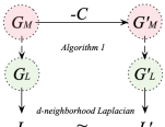
Figure 4: The construction considered in Definition 22. The node-pair $m$-$m^{\prime}$ is connected with distance $d$ in $G_{M}$, and disconnected in $G_{M}^{\prime}$, after dropping the edges of a cut $C$. For each linguistic graph, we consider it “local” Laplacian.

Definition 22.

Define a pair of meaning graphs $G$ and $G^{\prime}$, both with $n$ nodes and satisfying ball assumption $\text{$\mathcal{B}$}(d)$, with three properties: (1) $m\overset{d}{\leftrightsquigarrow}m^{\prime}$ in $G$, (2) $m\overset{}{\cancel{\leftrightsquigarrow}}m^{\prime}$ in $G^{\prime}$, (3) $E_{G^{\prime}}\subset E_{G}$, (4) $C=E_{G}\setminus E_{G^{\prime}}$ is an $(m,m^{\prime})$ min-cut of $G$.

Definition 23.

Define a distribution $\mathcal{G}$ over pairs of possible meaning graphs $G,G^{\prime}$ and pairs of nodes $m,m^{\prime}$ which satisfies the requirements of Definition 22. Formally, $\mathcal{G}$ is a uniform distribution over the following set: $$\{(G,G^{\prime},m,m^{\prime})\mid G,G^{\prime},m,m^{\prime}\text{satisfy Definition \ref{cut:construction}}\}.$$

As two linguistic graphs, we sample $G_{L}$ and $G^{\prime}_{L}$, as denoted in Figure 4. In the sampling of $G_{L}$ and $G^{\prime}_{L}$, all the edges share the randomization, except for the ones that correspond to $C$ (i.e., the difference between the $G_{M}$ and $G^{\prime}_{M}$). Let $\mathcal{U}$ be the union of the nodes involved in $\tilde{d}$-neighborhood of $w,w^{\prime}$, in $G_{L}$ and $G^{\prime}_{L}$. Define $L,L^{\prime}$ to be the Laplacian matrices corresponding to the nodes of $\mathcal{U}$. As $n$ grows, the two Laplacians become less distinguishable whenever $p_{-}\oplus\varepsilon_{-}$ and $d$ are large enough:

Lemma 24.

Let $c>0$ be a constant and $p_{-},\lambda$ be parameters of the sampling process in Algorithm 1 on a pair of meaning graphs $G$ and $G^{\prime}$ on $n$ nodes constructed according to Definition 22. Let $d\in\mathbb{N},\tilde{d}\geq\lambda d,$ and $L,L^{\prime}$ be the Laplacian matrices for the $\tilde{d}$-neighborhoods of the corresponding nodes in the sampled linguistic graphs $G_{L}$ and $\text{{$G_{L}$}}^{\prime}$. If ${\color[rgb]{0,0,0}{p_{-}\oplus\varepsilon_{-}}}\geq\frac{c\log n}{n}$ and $d>\log n,$ then, with a high probability, the two Laplacians are close: $$\vspace{-0.05cm}\|\tilde{L}-\tilde{L^{\prime}}\|\leq\frac{\sqrt{2\lambda}\,\text{$\mathcal{B}$}(1)}{\sqrt{n\log(n\lambda)}}\vspace{-0.05cm}$$

Proof of Lemma 24.

We start by proving an upper bound on $\tilde{L}-\tilde{L^{\prime}}$ in matrix inequality notation. Similar upper-bound holds for $\tilde{L^{\prime}}-\tilde{L}$ which concludes the theorem.

$$\tilde{L}-\tilde{L^{\prime}} =\frac{L}{\|{L}\|}-\frac{L^{\prime}}{\|L^{\prime}\|}$$

$$\preceq\frac{L}{\|L\|}-\frac{L^{\prime}}{\|L-L^{\prime}\|+\|L\|}$$

$$=\frac{L\cdot\|L-L^{\prime}\|}{\|L\|^{2}}+\frac{L-L^{\prime}}{\|L\|}$$

$$\preceq\frac{\sqrt{\lambda}\text{$\mathcal{B}$}(1)}{\sqrt{2n\log(n\lambda)}}I+\frac{\sqrt{\lambda}\text{$\mathcal{B}$}(1)}{\sqrt{2n\log(n\lambda)}}I.$$

The last inequality is due to Lemma 29. By symmetry the same upper-bound holds for $\tilde{L}^{\prime}-\tilde{L}\preceq 2\frac{\sqrt{\lambda}\text{$\mathcal{B}$}(1)}{\sqrt{2n\log(n\lambda)}}I$. This means that $\|\tilde{L}-\tilde{L}^{\prime}\|\leq\frac{2\sqrt{\lambda}\text{$\mathcal{B}$}(1)}{\sqrt{2n\log(n\lambda)}}$. ∎

This can be used to show that, for such large enough $p_{-}$ and $d$, the two linguistic graphs, $G_{L}$ and $G^{\prime}_{L}$ sampled as above, are indistinguishable by any function operating over a $\lambda d$-neighborhood of $w,w^{\prime}$ in $G_{L}$, with a high probability.

A reasoning function can be thought of a mapping defined on normalized Laplacians, since they encode all the information in a graph. For a reasoning function $f$ with limited precision, the input space can be partitioned into regions where the function is constant; and for large enough values of $n$ both $\tilde{L},\tilde{L}^{\prime}$ (with a high probability) fall into regions where $f$ is constant.

Note that a reasoning algorithm is oblivious to the the details of $C$, i.e. it does not know where $C$ is, or where it has to look for the changes. Therefore a realistic algorithm ought to use the neighborhood information collectively.

In the next lemma, we define a function $f$ to characterize the reasoning function, which uses Laplacian information and maps it to binary decisions. We then prove that for any such functions, there are regimes that the function won’t be able to distinguish $\tilde{L}$ and $\tilde{L}^{\prime}$:

Lemma 25.

Let meaning and linguistic graphs be constructed under the conditions of Lemma 24. Let $\beta>0$ and $f:\mathbb{R}^{|\mathcal{U}|\times|\mathcal{U}|}\rightarrow\{0,1\}$ be the indicator function of an open set. Then there exists $n_{0}\in\mathbb{N}$ such that for all $n\geq n_{0}$: $$\mathbb{P}_{\begin{subarray}{c}(G,G^{\prime},m,m^{\prime})\sim\mathcal{G}\\ G_{L}\leftarrow\mathsf{ALG}(G),\\ G^{\prime}_{L}\leftarrow\mathsf{ALG}(G^{\prime})\end{subarray}}\left[f(\tilde{L})=f(\tilde{L}^{\prime})\right]\geq 1-\beta.$$

Proof of Lemma 25.

Note that $f$ maps a high dimensional continuous space to a discrete space. To simplify the argument about $f$, we decompose it to two functions: a continuous function $g$ mapping matrices to $(0,1)$ and a threshold function $H$ (e.g. $0.5+0.5\text{sgn}(.)$) which maps to one if $g$ is higher than a threshold and to zero otherwise. Without loss of generality we also normalize $g$ such that the gradient is less than one. Formally,

$$f=H\circ g,\text{ where }g:\mathbb{R}^{|\mathcal{U}|\times|\mathcal{U}|}\rightarrow(0,1),\|\nabla g\Bigr{|}_{\tilde{L}}\|\leq 1.$$

Lemma 30 gives a proof of existence for such decompositon, which depends on having open or closed pre-images.

One can find a differentiable and Lipschitz function $g$ such that it intersects with the threshold specified by $H$, in the borders where $f$ changes values.

With $g$ being Lipschitz, one can upper-bound the variations on the continuous function:

$$\|g(\tilde{L})-g(\tilde{L^{\prime}})\|\leq M\|\tilde{L}-\tilde{L}^{\prime}\|.$$

According to Lemma 24, $\|\tilde{L}-\tilde{L}^{\prime}\|$ is upper-bounded by a decreasing function in $n$.

For uniform choices $(G,G^{\prime},m,m^{\prime})\sim\mathcal{G}$ (Definition 23) the Laplacian pairs $(\tilde{L},\tilde{L}^{\prime})$ are randomly distributed in a high-dimensional space, and for big enough $n$, there are enough portion of the $(\tilde{L},\tilde{L}^{\prime})$ (to satisfy $1-\beta$ probability) that appear in the same side of the hyper-plane corresponding to the threshold function (i.e. $f(\tilde{L})=f(\tilde{L}^{\prime})$). ∎

Proof of Theorem 13.

By substituting $\gamma=\beta$, and $X_{L}=f$, the theorem reduces to the statement of Lemma 25.

∎

E.2 Auxiliary Lemmas and Proofs

In the following lemma, we show that the spectral differences between the two linguistic graphs in the locality of the target nodes are small. For ease of exposition, we define an intermediate notation, for a normalized version of the Laplacians: $\tilde{L}=L/\|L\|_{2}$ and $\tilde{L}^{\prime}=L^{\prime}/\|L^{\prime}\|_{2}$.

Lemma 26.

The norm-2 of the Laplacian matrix corresponding to the nodes participating in a cut, can be upper-bounded by the number of the edges participating in the cut (with a constant factor).

Proof of Lemma 26.

Using the definition of the Laplacian:

$$\|L_{C}\|_{2}\leq\|A-D\|_{2}\leq\|A\|_{2}+\|D\|_{2}$$

where $A$ is the adjacency matrix and $D$ is a diagonal matrix with degrees on the diagonal. We bound the norms of the matrices based on size of the cut (i.e., number of the edges in the cut). For the adjacency matrix we use the Frobenius norm:

$$\|A\|_{2}\leq\|A\|_{F}=\sqrt{\sum_{ij}a_{ij}}=2\cdot|C|$$

where $|C|$ denotes the number of edges in $C$. To bound the matrix of degrees, we use the fact that norm-2 is equivalent to the biggest eigenvalue, which is the biggest diagonal element in a diagonal matrix:

$$\|D\|_{2}=\sigma_{\max}(D)=\max_{i}deg(i)\leq|C|$$

With this we have shown that: $\|L_{C}\|_{2}\leq 3|C|$. ∎

For sufficiently large values of $p$, $\mathsf{G(n,p)}$ is a connected graph, with a high probability. More formally:

Lemma 27 (Connectivity of random graphs).

In a random graph $\mathsf{G(n,p)}$, for any $p$ bigger than ${{\tfrac{(1+\varepsilon)\ln n}{n}}}$, the graph will almost surely be connected. The proof can be found in Erdos and Rényi (1960).

Lemma 28 (Norm of the adjacency matrix in a random graph).

For a random graph $\mathsf{G(n,p)}$, let $L$ be the adjacency matrix of the graph. For any $\varepsilon>0$: $$\lim_{n\rightarrow+\infty}\mathbb{P}\left(\left|\|L\|_{2}-\sqrt{2n\log n}\right|>\varepsilon\right)\rightarrow 0$$

Proof of Lemma 28.

From Theorem 1 of Ding et al. (2010) we know that:

$$\frac{\sigma_{\max}{(L)}}{\sqrt{n\log n}}\overset{P}{\rightarrow}\sqrt{2}$$

where $\overset{P}{\rightarrow}$ denote convergence in probability. And also notice that norm-2 of a matrix is basically the size of its biggest eigenvalue, which concludes our proof. ∎

Lemma 29.

For any pair of meaning-graphs $G$ and $G^{\prime}$ constructed according to Definition 22, and, • $d>\log n$, • $p_{-}\oplus\varepsilon_{-}\geq c\log n\big{/}n$ for some constant $c$, • $\tilde{d}\geq\lambda d$, with $L$ and $L^{\prime}$ being the Laplacian matrices corresponding to the $\tilde{d}$-neighborhoods of the corresponding nodes in the surface-graph; we have: $$\frac{\|L-L^{\prime}\|_{2}}{\|L\|_{2}}\leq\frac{\sqrt{\lambda}\text{$\mathcal{B}$}(1)}{\sqrt{2n\log(n\lambda)}},$$ with a high-probability.

Proof of Lemma 29.

In order to simplify the exposition, w.l.o.g. assume that $\varepsilon_{-}=0$ (see Remark 9). Our goal is to find an upper-bound to the fraction $\frac{\|L-L^{\prime}\|_{2}}{\|L\|_{2}}$. Note that the Laplacians contain only the local information, i.e., $\tilde{d}-$neighborhood. First we prove an upper bound on the nominator. By eliminating an edge in a meaning-graph, the probability of edge appearance in the linguistic graph changes from $p_{+}$ to $p_{-}$. The effective result of removing edges in $C$ would appear as i.i.d. $\text{Bern}(p_{+}-p_{-})$. Since by definition, $\text{$\mathcal{B}$}(1)$ is an upper bound on the degree of meaning nodes, the size of minimum cut should also be upper bounded by $\mathcal{B}$(1). Therefore, the maximum size of the min-cut $C$ separating two nodes $m\overset{d}{\leftrightsquigarrow}m^{\prime}$ is at most $\text{$\mathcal{B}$}(1)$. To account for vertex replication in linguistic graph, the effect of cut would appear on at most $\lambda\text{$\mathcal{B}$}(1)$ edges in the linguistic graph. Therefore, we have$\|L-L^{\prime}\|_{2}\leq\lambda\text{$\mathcal{B}$}(1)$ using Lemma 26.

As for the denominator, the size of the matrix $L$ is the same as the size of $\tilde{d}$-neighborhood in the linguistic graph. We show that if $\tilde{d}>\log(\lambda n)$ the neighborhood almost-surely covers the whole graph. While the growth in the size of the $\tilde{d}$-neighborhood is a function of both $p_{+}$ and $p_{-}$, to keep the analysis simple, we underestimate the neighborhood size by replacing $p_{+}$ with $p_{-}$, i.e., the size of the $\tilde{d}$-neighborhood is lower-bounded by the size of a $\tilde{d}$-neighborhood in $\mathsf{G}(\lambda\cdot n,p_{-})$.

By Lemma 27 the diameters of the linguistic graphs $G_{L}$ and $G_{L}^{\prime}$ are both $\Theta(\log(\lambda n))$. Since $\tilde{d}\in\Omega(\log(\lambda n))$, $\tilde{d}$-neighborhood covers the whole graph for both $G_{L}$ and $G_{L}^{\prime}$.

Next, we use Lemma 28 to state that $\|L\|_{2}$ converges to $\sqrt{2\lambda n\log(\lambda n)}$, in probability.

Combining numerator and denominator, we conclude that the fraction, for sufficiently large $n$, is upper-bounded by: $\frac{\lambda\text{$\mathcal{B}$}(1)}{\sqrt{2\lambda n\log(\lambda n)}},$ which can get arbitrarily small, for a big-enough choice of $n$. ∎

Lemma 30.

Suppose $f$ is an indicator function on an open set, it is always possible to write it as composition of two functions: • A continuous and Lipschitz function: $g:\mathbb{R}^{d}\rightarrow(0,1),$ • A thresholding function: $H(x)=\mathbf{1}\{x>0.5\}.$ such that: $\forall x\in\mathbb{R}^{d}:\;\;\;f(x)=h(g(x))$.

Proof of Lemma 30.

Without loss of generality, we assume that the threshold function is defined as $H(x)=\mathbf{1}\{x>0.5\}$. One can verify that a similar proof follows for $H(x)=\mathbf{1}\{x\geq 0.5\}$. We use notation $f^{-1}(A)$ the set of pre-images of a function $f$, for the set of outputs $A$.

First let’s study the collection of inputs that result in output of $1$ in $f$ function. Since $f=h\circ g$, then $f^{-1}(\{1\})=g^{-1}(h^{-1}(\{1\}))=g^{-1}((0.5,1))$ and $f^{-1}(\{0\})=g^{-1}(h^{-1}(\{0\}))=g^{-1}((0,0.5))$. Define $C_{0}$ and $C_{1}$, such that $C_{i}\triangleq f^{-1}(\{i\})$; note that since $g$ is continuous and $(0.5,1)$ is open $C_{1}$ is an open set (hence $C_{1}$ is closed). Let $d:\mathbb{R}^{n}\to\mathbb{R}$ be defined by,

$$d(x)\triangleq\text{dist}(x,C_{0})=\inf_{c\in C_{0}}\|x-c\|.$$

Since $C_{0}$ is closed, it follows $d(x)=0$ if and only if $x\in C_{0}$. Therefore, letting

$$g(x)=\frac{1}{2}+\frac{1}{2}\cdot\frac{d(x)}{1+d(x)},$$

then $g(x)=\frac{1}{2}$ when $x\in C_{0}$, while $g(x)>\frac{1}{2}$ when $x\not\in C_{0}$. This means that letting $h(x)=1$ when $x>\frac{1}{2}$ and $h(x)=0$ when $x\leq\frac{1}{2}$, then $f=h\circ g$. One can also verify that this construction is $1/2$-Lipschitz; this follows because $d(x)$ is $1$-Lipschitz, which can be proved using the triangle inequality

Hence the necessary condition to have such decomposition is $f^{-1}(\{1\})$ and $f^{-1}(\{0\})$ be open or closed. ∎

Appendix F Empirical investigation: further details

To evaluate the impact of the other noise parameters in the sampling process, we compare the average distances between nodes in the linguistic graph for a given distance between the meaning graph nodes. In the Figure 5, we plot these graphs for decreasing values of $p_{-}$ (from top left to bottom right). With high $p_{-}$ (top left subplot), nodes in the linguistic graph at distances lower than two, regardless of the distance of their corresponding node-pair in the meaning graph. As a result, any reasoning algorithm that relies on connectivity can not distinguish linguistic nodes that are connected in the meaning space from those that are not. As the $p_{-}$ is set to lower values (i.e. noise reduces), the distribution of distances get wider, and correlation of distance between the two graphs increases. In the bottom middle subplot, when $p_{-}$ has a very low value, we observe a significant correlation that can be reliably utilized by a reasoning algorithm.

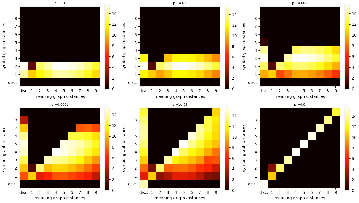
Figure 5: With varied values for $p_{-}$ a heat map representation of the distribution of the average distances of node-pairs in linguistic graph based on the distances of their corresponding meaning nodes is presented.

References

• Angeli and Manning (2014) Gabor Angeli and Christopher D. Manning. 2014. Naturalli: Natural logic inference for common sense reasoning. In EMNLP.
• Bollacker et al. (2008) Kurt Bollacker, Colin Evans, Praveen Paritosh, Tim Sturge, and Jamie Taylor. 2008. Freebase: A collaboratively created graph database for structuring human knowledge. In ICMD, pages 1247–1250. ACM.
• Chung and Lu (2002) Fan Chung and Linyuan Lu. 2002. The average distances in random graphs with given expected degrees. Proceedings of the National Academy of Sciences, 99(25):15879–15882.
• Cormen et al. (2009) Thomas H Cormen, Charles E Leiserson, Ronald L Rivest, and Clifford Stein. 2009. Introduction to algorithms. MIT press.
• Devlin et al. (2019) Jacob Devlin, Ming-Wei Chang, Kenton Lee, and Kristina Toutanova. 2019. BERT: Pre-training of deep bidirectional transformers for language understanding. In NAACL-HLT.
• Ding et al. (2010) Xue Ding, Tiefeng Jiang, et al. 2010. Spectral distributions of adjacency and laplacian matrices of random graphs. The annals of applied probability, 20(6):2086–2117.
• Erdos and Rényi (1960) Paul Erdos and Alfréd Rényi. 1960. On the evolution of random graphs. Publ. Math. Inst. Hung. Acad. Sci, 5(1):17–60.
• Fried et al. (2015) Daniel Fried, Peter Jansen, Gustave Hahn-Powell, Mihai Surdeanu, and Peter Clark. 2015. Higher-order lexical semantic models for non-factoid answer reranking. TACL, 3.
• Gilbert (1959) Edgar N Gilbert. 1959. Random graphs. The Annals of Mathematical Statistics, 30(4):1141–1144.
• Harnad (1990) Stevan Harnad. 1990. The symbol grounding problem. Physica D: Nonlinear Phenomena, 42(1-3):335–346.
• Jansen et al. (2016) Peter Jansen, Niranjan Balasubramanian, Mihai Surdeanu, and Peter Clark. 2016. What’s in an explanation? characterizing knowledge and inference requirements for elementary science exams. In COLING, pages 2956–2965.
• Jansen et al. (2017) Peter Jansen, Rebecca Sharp, Mihai Surdeanu, and Peter Clark. 2017. Framing qa as building and ranking intersentence answer justifications. Computational Linguistics.
• Jansen (2016) Peter A Jansen. 2016. A study of automatically acquiring explanatory inference patterns from corpora of explanations: Lessons from elementary science exams. In AKBC.
• Jansen et al. (2018) Peter A. Jansen, Elizabeth Wainwright, Steven Marmorstein, and Clayton T. Morrison. 2018. WorldTree: A corpus of explanation graphs for elementary science questions supporting multi-hop inference. In LREC.
• Johnson-Laird (1980) Philip Nicholas Johnson-Laird. 1980. Mental models in cognitive science. Cognitive science, 4(1):71–115.
• Khashabi et al. (2016) Daniel Khashabi, Tushar Khot, Ashish Sabharwal, Peter Clark, Oren Etzioni, and Dan Roth. 2016. Question answering via integer programming over semi-structured knowledge. In IJCAI.
• Khot et al. (2017) Tushar Khot, Ashish Sabharwal, and Peter Clark. 2017. Answering complex questions using open information extraction. ACL.
• Lin et al. (2018) Xi Victoria Lin, Richard Socher, and Caiming Xiong. 2018. Multi-hop knowledge graph reasoning with reward shaping. In EMNLP.
• McCarthy (1963) John McCarthy. 1963. Programs with common sense. Defense Technical Information Center.
• Mihalcea and Csomai (2007) Rada Mihalcea and Andras Csomai. 2007. Wikify!: linking documents to encyclopedic knowledge. In CIKM, pages 233–242.
• Mihaylov et al. (2018) Todor Mihaylov, Peter Clark, Tushar Khot, and Ashish Sabharwal. 2018. Can a suit of armor conduct electricity? a new dataset for open book question answering. In EMNLP.
• Mikolov et al. (2013) Tomas Mikolov, Kai Chen, Greg Corrado, and Jeffrey Dean. 2013. Efficient estimation of word representations in vector space. In ICLR.
• Milgram (1967) Stanley Milgram. 1967. Six degrees of separation. Psychology Today, 2:60–64.
• Miller (1995) George Miller. 1995. Wordnet: a lexical database for english. Communications of the ACM, 38(11):39–41.
• Pearl (1988) J Pearl. 1988. Probabilistic Reasoning in Intelligent Systems: Networks of Plausible Inference. Morgan Kaufmann Publishers Inc., San Francisco, CA, USA.
• Peters et al. (2018) Matthew E. Peters, Mark Neumann, Mohit Iyyer, Matt Gardner, Christopher Clark, Kenton Lee, and Luke S. Zettlemoyer. 2018. Deep contextualized word representations. In NAACL.
• Punyakanok et al. (2004) Vasin Punyakanok, Dan Roth, and Scott Yih. 2004. Mapping dependencies trees: An application to question answering. AIM.
• Quillan (1966) M Ross Quillan. 1966. Semantic memory. Technical report, Bolt Beranek and Newman Inc, Cambridge, MA.
• Ratinov et al. (2011) Lev Ratinov, Dan Roth, Doug Downey, and Mike Anderson. 2011. Local and global algorithms for disambiguation to Wikipedia. In ACL.
• Reddy et al. (2017) Siva Reddy, Oscar Täckström, Slav Petrov, Mark Steedman, and Mirella Lapata. 2017. Universal semantic parsing. In EMNLP, pages 89–101.
• Socher et al. (2013) Richard Socher, Danqi Chen, Christopher D. Manning, and Andrew Y. Ng. 2013. Reasoning with neural tensor networks for knowledge base completion. In NIPS.
• Steedman and Baldridge (2011) Mark Steedman and Jason Baldridge. 2011. Combinatory categorial grammar. Non-Transformational Syntax: Formal and explicit models of grammar, pages 181–224.
• Taddeo and Floridi (2005) Mariarosaria Taddeo and Luciano Floridi. 2005. Solving the symbol grounding problem: a critical review of fifteen years of research. Journal of Experimental & Theoretical Artificial Intelligence, 17(4):419–445.
• Toutanova and Chen (2015) Kristina Toutanova and Danqi Chen. 2015. Observed versus latent features for knowledge base and text inference. In Workshop on Continuous Vector Space Models and their Compositionality (CVSC).
• Yang et al. (2018) Zhilin Yang, Peng Qi, Saizheng Zhang, Yoshua Bengio, William W. Cohen, Ruslan Salakhutdinov, and Christopher D. Manning. 2018. HotpotQA: A dataset for diverse, explainable multi-hop question answering. In EMNLP.
Supplemental Material