Efficient Minimum Distance Estimation of Pareto Exponent from Top Income Shares

Abstract

We propose an efficient estimation method for the income Pareto exponent when only certain top income shares are observable. Our estimator is based on the asymptotic theory of weighted sums of order statistics and the efficient minimum distance estimator. Simulations show that our estimator has excellent finite sample properties. We apply our estimation method to U.S. top income share data and find that the Pareto exponent has been stable at around 1.5 since 1985, suggesting that the rise in inequality during the last three decades is mainly driven by redistribution between the rich and poor, not among the rich.

Keywords: minimum distance estimator, order statistics, power law.

JEL codes: C46.

1 Introduction

It is well-known that the income distribution as well as many other size distributions of economic interest exhibit Pareto (power law) tails, meaning that the tail probability $P(X>x)$ decays like a power function $x^{-\alpha}$ for large $x$, where $\alpha>0$ is called the Pareto exponent. Oftentimes, knowing the Pareto exponent $\alpha$ is of considerable practical interest because it determines the shape of the income distribution for the rich and hence income inequality. As a motivating example, consider the theory of optimal taxation. If the government’s objective is to maximize the total tax revenue, then Saez (2001) shows that the optimal income tax rate is $\tau=\frac{1}{1+\alpha e}$, where $\alpha$ is the income Pareto exponent and $e$ is the elasticity of income in the top bracket with respect to the tax rate. If we set $e=0.3$ as estimated by Piketty et al. (2014) and $\alpha=1.5$–$3$ as is often reported, then the optimal tax rate ranges from 70% when $\alpha=1.5$ and 53% when $\alpha=3$. Clearly, the knowledge of the Pareto exponent is important for policy design.

When individual data on income is available, it is relatively straightforward to estimate and conduct inference on the Pareto exponent, either by maximum likelihood (Hill, 1975), log rank regressions (Gabaix and Ibragimov, 2011), fixed-$k$ asymptotics (Müller and Wang, 2017), or other methods. Even if individual data is not available, if we have binned data we can still estimate the Pareto exponent by eyeballing (Pareto, 1897) or maximum likelihood (Virkar and Clauset, 2014). However, in practice it is often the case (especially for administrative data) that only some top income shares are reported and individual data are not available. A typical example is Table 1 below, which summarizes the U.S. household income distribution. Such income data in the form of tabulations are quite common, including the World Inequality Database.

Table 1: U.S. top income shares (%).

Year	Top income percentiles
	0.01	0.1	0.5	1	5	10
1917	3.37	8.40	14.34	17.74	30.64	40.51
⋮	⋮	⋮	⋮	⋮	⋮	⋮
2017	4.95	10.43	17.16	21.47	38.14	50.14

Existing studies of such income share data typically rely on some parametric assumption of the whole distribution. Given a parametric density, the income shares can be expressed as functions of the unknown parameters and then be estimated by moment-based estimators. Statistical inference is constructed by either using the asymptotic normality or bootstrapping. For example, McDonald (1984) and Kleiber and Kotz (2003) propose to use the generalized beta type-II distribution (GB2) to approximate the whole income distribution. Under this assumption, Chotikapanich et al. (2007), Chotikapanich et al. (2012), and Hajargasht et al. (2012) develop moment-based estimators and inference methods for grouped mean and share data, and Chen (2018) further constructs a unified framework that allows for general form of grouped data. These methods all focus on the mid-sample moments, which can be expressed as known functions of the parameters of the GB2 distribution.

However, the parametric assumption on the whole distribution may lead to a substantial misspecification error when the object of interest is in the tail. This is because tail properties such as very large quantiles are typically in a large scale, and hence a small misspecification in mid-sample can be amplified by a large factor in the tail. For example, the standard normal distribution and the Student-$t$ distribution with degree of freedom 20 share almost the same shape in mid-sample but exhibit substantially different top quantiles. Such misspecification is documented by Brzezinski (2013) in an extensive simulation study.

In addition to the potential misspecification in mid-sample, there is another source of bias when studying tail related objects, which is the dependence among large order statistics. Suppose we are interested in the right tail of the underlying distribution. Then essentially only the largest order statistics are informative. Even if the observations are independent, the largest order statistics are not. Such dependence may incur a large misspecification error again if it is ignored, especially when the very top income share such as 0.01% is considered. For example, think of the population size as $10^{5}$. The top 0.01% share involves only the ten largest order statistics, whose distribution has to be jointly modeled to capture the dependence.

In this paper, we focus only on the top income shares and propose an efficient estimation method for the Pareto exponent. Compared with existing methods, the new estimator takes into consideration of the dependence among large order statistics and is robust to misspecification in mid-sample. In particular, our method is based on the following observations. By definition, top income shares are the ratios between the sum of order statistics for some top percentile and total income. Assuming that the upper tail of the income distribution is Pareto, we derive the joint asymptotic distribution of normalized top income shares using the results on the weighted sums of order statistics due to Stigler (1974). From this result, we define the classical minimum distance (CMD) estimator (Chiang, 1956; Ferguson, 1958) and derive its asymptotic properties.

More specifically, we typically cannot identify the shape of the underlying distribution without observing individual data. However, if we assume the sample size is large enough (but not necessarily known) and the underlying distribution has a Pareto upper tail, we can show that the top shares are jointly asymptotically Gaussian with the mean vector and the variance-covariance matrix being characterized by the Pareto exponent and the scale parameter. Since the scale parameter is not identified given only the shares, we eliminate it by imposing scale invariance and considering a self-normalized statistic, whose distribution is still jointly normal but now fully characterized by the Pareto exponent only. Thus, the problem is asymptotically equivalent to estimating a single parameter in a joint normal distribution using a single random draw from it. The efficient solution is then to consider the continuously updated minimum distance estimator (CUMDE). As we show in simulations, this estimator has excellent finite sample properties when the model is correctly specified.

We note that the Pareto assumption is required for the tail only instead of the whole income distribution, which is why our method is robust to misspecification in mid-sample. In particular, when the data generating process is not exactly Pareto, our estimator still performs well when we only use small enough top percentiles such as the top 1% and the sample size is large enough, which is typically the case for income share data based on tax returns (where the number of households is in the order of a million).

We apply our new method to estimate the income Pareto exponent in U.S. and France. In U.S., we estimate that the income Pareto exponent has decreased from about 2.2 in 1975 to about 1.6 in 1985, which has remained relatively stable since then at around 1.5 with a conservative 95% confidence interval of length no more than 0.1. This finding is in stark contrast to other inequality measures such as the top 1% income share, which has increased from about 10% in 1985 to 20% at present, and suggests that the rise in inequality during the last three decades is mainly driven by redistribution between the rich and poor, not among the rich. In France, we find that the Pareto exponent is stable at around 2 postwar.

2 Weighted sums of order statistics

In this section we derive the asymptotic distribution of the weighted sums of order statistics of a Pareto distribution, which we subsequently use to construct the estimator of the Pareto exponent.

Let $\left\{{Y_{i}}\right\}_{i=1}^{n}$ be independent and identically distributed (i.i.d.) copies of a positive random variable $Y$ with cumulative distribution function (CDF) $F(y)$ and density $f(y)=F^{\prime}(y)$. Let

$$Y_{(1)}\geq\dots\geq Y_{(n)}$$

denote the order statistics. Following Stigler (1974), consider the weighted sum

$$L_{n}=\frac{1}{n}\sum_{i=1}^{n}J\left(\frac{i}{n+1}\right)Y_{(n-i+1)},$$

where $J:[0,1]\to\mathbb{R}$ is a function that is bounded and continuous almost everywhere with respect to the Lebesgue measure. When

$$J(x)=1[1-q<x\leq 1-p]$$ (2.1)

for some $0<p<q\leq 1$, $L_{n}$ can be interpreted as the sum of $Y_{(i)}$’s between the top $100p$ and $100q$ percentiles, divided by the sample size $n$.

The following lemma shows that $L_{n}$ is asymptotically normal.

Lemma 2.1.

Let $J$ be as in (2.1). Then

$$\sqrt{n}(L_{n}-\mu(J,F))\xrightarrow{\mathrm{d}}N(0,\sigma^{2}(J,F)),$$

where

$$\mu(J,F) =\int_{0}^{1}J(x)F^{-1}(x)\mathop{}\!\mathrm{d}x,$$ (2.2a)

$$\sigma^{2}(J,F) =\int_{0}^{1}\int_{0}^{1}\frac{J(x_{1})J(x_{2})}{f(F^{-1}(x_{1}))f(F^{-1}(x_{2}))}(\min\left\{{x_{1},x_{2}}\right\}-x_{1}x_{2})\mathop{}\!\mathrm{d}x_{1}\mathop{}\!\mathrm{d}x_{2}.$$ (2.2b)

Proof.

The statement follows from Stigler (1974, Theorem 5) and the change of variable $x=F(y)$. Note that $J(x)=1[1-q<x\leq 1-p]$ implies $J(x)=0$ for $x>1-p$. ∎

In the remainder of the paper, we assume that $Y$ is Pareto distributed with Pareto exponent $\alpha>1$ and minimum size $c>0$, so $F(y)=1-(y/c)^{-\alpha}$ for $y\geq c$. The Pareto exponent $\alpha$ captures the shape and the minimum size $c$ characterizes the scale. By simple algebra, we obtain

$$f(y) =F^{\prime}(y)=\alpha c^{\alpha}y^{-\alpha-1},$$ (2.3a)

$$F^{-1}(x) =c(1-x)^{-1/\alpha},$$ (2.3b)

$$f(F^{-1}(x)) =\frac{\alpha}{c}(1-x)^{1+1/\alpha}.$$ (2.3c)

When $Y$ is Pareto distributed, we can explicitly compute the moments in Lemma 2.1 as follows.

Lemma 2.2.

Let $J$ be as in (2.1) and $F$ be the Pareto CDF with exponent $\alpha>1$ and minimum size $c$. Letting $\xi=1/\alpha<1$, we have

$$\mu(J,F)=\mu(p,q)\coloneqq c\frac{q^{1-\xi}-p^{1-\xi}}{1-\xi},$$ (2.4a)

$$\sigma^{2}(J,F)=\sigma^{2}(p,q)$$

$$\coloneqq\frac{2c^{2}\xi^{2}}{1-\xi}\left(\frac{q^{1-2\xi}-p^{1-2\xi}}{1-2\xi}+p^{1-\xi}\frac{q^{-\xi}-p^{-\xi}}{\xi}+\frac{2p^{1-\xi}q^{1-\xi}-p^{2-2\xi}-q^{2-2\xi}}{2-2\xi}\right),$$ (2.4b)

where $\frac{q^{1-2\xi}-p^{1-2\xi}}{1-2\xi}$ is interpreted as $\log\frac{q}{p}$ if $\xi=1/2$.

Next, we consider the joint distribution of the sums of $Y_{(i)}$’s over some top percentile groups. Suppose that there are $K$ groups indexed by $k=1\dots,K$, and the $k$-th group corresponds to the top $p_{k}$ to $p_{k+1}$ percentile, where $0<p_{1}<\dots<p_{K}<p_{K+1}\leq 1$. Define

$$\bar{Y}_{k}=\frac{1}{n}\sum_{i=\left\lfloor np_{k}\right\rfloor+1}^{\left\lfloor np_{k+1}\right\rfloor}Y_{(i)},$$ (2.5)

where $\left\lfloor x\right\rfloor$ denotes the largest integer not exceeding $x$. By Lemmas 2.1 and 2.2, we have

$$\sqrt{n}(\bar{Y}_{k}-\mu_{k})\xrightarrow{\mathrm{d}}N(0,\sigma_{k}^{2}),$$

where $\mu_{k}=\mu(p_{k},p_{k+1})$ and $\sigma_{k}^{2}=\sigma^{2}(p_{k},p_{k+1})$ are given by (2.4a) and (2.4b), respectively. Let $\bar{Y}=(\bar{Y}_{1},\dots,\bar{Y}_{K})^{\top}$ and $\mu=(\mu_{1},\dots,\mu_{K})^{\top}$. Then by the Cramér-Wold device, it follows that

$$\sqrt{n}(\bar{Y}-\mu)\xrightarrow{\mathrm{d}}N(0,\Sigma),$$ (2.6)

where $\Sigma$ is some variance matrix with $\Sigma_{kk}=\sigma_{k}^{2}$. The following lemma gives an explicit formula for $\Sigma$.

Lemma 2.3.

The variance matrix $\Sigma$ in (2.6) is symmetric and

$$\Sigma_{jk}=\begin{cases}\sigma_{k}^{2}=\sigma^{2}(p_{k},p_{k+1}),&(j=k)\\ -c^{2}\xi^{2}\frac{p_{j+1}^{1-\xi}-p_{j}^{1-\xi}}{1-\xi}\left(\frac{p_{k+1}^{-\xi}-p_{k}^{-\xi}}{\xi}+\frac{p_{k+1}^{1-\xi}-p_{k}^{1-\xi}}{1-\xi}\right).&(j<k)\end{cases}$$ (2.7)

Furthermore, $\Sigma$ is positive definite.

3 Minimum distance estimator

In practice, the income distribution is often presented as a tabulation of top income shares as in Table 1 and micro data is not available. In this case the researcher is forced to conduct inference on the Pareto exponent $\alpha$ based on the top income shares of the given top percentiles, for example

$$p=(p_{1},p_{2},p_{3},p_{4},p_{5},p_{6})=\frac{1}{100}(0.01,0.1,0.5,1,5,10)$$ (3.1)

as in Table 1. If $Y$ is distributed as Pareto with exponent $\alpha>1$ and minimum size $c>0$, using $F(y)=1-(y/c)^{-\alpha}$, the population top $p$ percentile is

$$1-(y/c)^{-\alpha}=1-p\iff y=cp^{-1/\alpha}.$$

Using (2.3a), the total income held by the population top $p$ percentile is

$$Y(p)\coloneqq\int_{cp^{-1/\alpha}}^{\infty}y\alpha c^{\alpha}y^{-\alpha-1}\mathop{}\!\mathrm{d}y=c\frac{\alpha}{\alpha-1}p^{1-1/\alpha}.$$

Therefore the population top $p$ income share is

$$S(p)\coloneqq Y(p)/Y(1)=p^{1-1/\alpha},$$

which depends only on $p$ and $\alpha$. If $Y$ is Pareto only for the upper tail, a similar calculation yields

$$S(p)/S(q)=(p/q)^{1-1/\alpha}\iff\alpha=\frac{1}{1-\frac{\log(S(q)/S(p))}{\log(q/p)}}$$ (3.2)

for $0<p<q\ll 1$. Atkinson and Piketty (2010, Table 13A.23) and Aoki and Nirei (2017, Figure 3) estimate the income Pareto exponents from (3.2) using $p=0.1\%$ and $q=1\%$. A natural question is whether such a method can be statistically justified for the tabulation data as in Table 1. In this section, we derive such an estimator and discuss its asymptotic properties.

3.1 Asymptotic theory

Let $\left\{{Y_{i}}\right\}_{i=1}^{n}$ be the (unobserved) income data and $Y_{(1)}\geq\dots\geq Y_{(n)}$ the order statistics. Let $K\geq 2$ and suppose that some top percentiles $0<p_{1}<\dots<p_{K}<p_{K+1}\leq 1$ and the corresponding sample top income shares

$$S_{k}=\frac{\sum_{i=1}^{\left\lfloor np_{k}\right\rfloor}Y_{(i)}}{\sum_{i=1}^{n}Y_{(i)}},\quad k=1,\dots,K+1,$$

are given. Suppose that $p_{K+1}$ is small enough such that for $i\leq\left\lfloor np_{K+1}\right\rfloor$, we may assume that $Y_{(i)}$ are realizations from a Pareto distribution with exponent $\alpha$ and minimum size $c$. To construct an estimator of $\alpha$ based only on $\left\{{S_{k}}\right\}$, we consider the vector of self-normalized non-overlapping top income shares defined by

$$\bar{s}=(\bar{s}_{1},\dots,\bar{s}_{K-1})^{\top}\coloneqq\left(\frac{S_{2}-S_{1}}{S_{K+1}-S_{K}},\dots,\frac{S_{K}-S_{K-1}}{S_{K+1}-S_{K}}\right)^{\top}.$$ (3.3)

The following proposition shows that $\bar{s}$ is asymptotically normal.

Proposition 3.1.

Let $r_{k}=\mu_{k}/\mu_{K}$, where $\mu_{k}=\mu(p_{k},p_{k+1})$ is given by (2.4a). Define the $(K-1)$-vector $r=(r_{1},\dots,r_{K-1})^{\top}$ and $(K-1)\times K$ matrix $H=\begin{bmatrix}I_{K-1}&-r\end{bmatrix}/\mu_{K}$. Then

$$\sqrt{n}(\bar{s}-r)\xrightarrow{\mathrm{d}}N(0,H\Sigma H^{\top}).$$

The variance matrix $\Omega(\alpha)\coloneqq H\Sigma H^{\top}$ depends only on $\alpha$ and is positive definite.

Based on Proposition 3.1, it is natural to consider the classical minimum distance (CMD) estimator (Chiang, 1956; Ferguson, 1958)

$$\widehat{\alpha}=\operatornamewithlimits{arg\,min}_{\alpha\in A}(r(\alpha)-\bar{s})^{\top}\widehat{W}(r(\alpha)-\bar{s}),$$ (3.4)

where $\widehat{W}$ is some symmetric and positive definite weighting matrix and $A$ is some compact parameter space.

Let $G_{n}(\alpha)$ be the objective function in (3.4). Suppose that $\widehat{W}\xrightarrow{\mathrm{p}}W$ as $n\to\infty$, where $W$ is also positive definite. Letting $\alpha_{0}\in A$ be the true Pareto exponent, we have

$$G_{n}(\alpha)\xrightarrow{\mathrm{p}}G(\alpha)\coloneqq(r(\alpha)-r(\alpha_{0}))^{\top}W(r(\alpha)-r(\alpha_{0})).$$

Since $W$ is positive definite, we have $G(\alpha)\geq 0=G(\alpha_{0})$, with equality if and only if $r(\alpha)=r(\alpha_{0})$. The following proposition shows that the parameter $\alpha$ is point-identified by this condition.

Proposition 3.2 (Identification).

$\alpha\neq\alpha_{0}$ implies $r(\alpha)\neq r(\alpha_{0})$.

Using standard arguments, consistency and asymptotic normality follows from the above identification result.

Theorem 3.3 (Consistency).

Let $A\subset(1,\infty)$ be compact, $\alpha_{0}\in A$, and suppose $\widehat{W}\xrightarrow{\mathrm{p}}W$ as $n\to\infty$, where $W$ is positive definite. Let $\widehat{\alpha}$ be the minimum distance estimator in (3.4). Then $\widehat{\alpha}\xrightarrow{\mathrm{p}}\alpha_{0}$.

Proof.

Clearly $G(\alpha)$ is continuous in $\alpha>1$. The statement follows from Proposition 3.2, the uniform law of large numbers, and Newey and McFadden (1994, Theorem 2.1). ∎

Theorem 3.4 (Asymptotic normality).

Let $r(\alpha),\Omega(\alpha)$ be defined as in Proposition 3.1. Suppose that the assumptions of Theorem 3.3 hold and $\alpha_{0}$ is an interior point of $A$. Then

$$\sqrt{n}(\widehat{\alpha}-\alpha_{0})\xrightarrow{\mathrm{d}}N(0,V)$$

as $n\to\infty$, where

$$V=(R^{\top}WR)^{-1}R^{\top}W\Omega WR(R^{\top}WR)^{-1}$$

for $\Omega=\Omega(\alpha_{0})$ and $R=\nabla r(\alpha_{0})$.

Proof.

Immediate from Theorem 3.3 and Newey and McFadden (1994, Theorem 3.2). ∎

By standard results in classical minimum distance estimation (Chiang, 1956; Ferguson, 1958), we achieve efficiency by choosing the weighting matrix such that $\widehat{W}\xrightarrow{\mathrm{p}}W=\Omega^{-1}$. Therefore the most natural estimator is the following continuously updated minimum distance estimator (CUMDE).

Corollary 3.5 (Efficient CMD).

Let everything be as in Theorem 3.4 and define the continuously updated minimum distance estimator (CUMDE) by

$$\widehat{\alpha}=\operatornamewithlimits{arg\,min}_{\alpha\in A}(r(\alpha)-\bar{s})^{\top}\Omega(\alpha)^{-1}(r(\alpha)-\bar{s}),$$ (3.5)

where $\Omega(\alpha)$ is given as in Proposition 3.1. Then

$$\sqrt{n}(\widehat{\alpha}-\alpha_{0})\xrightarrow{\mathrm{d}}N(0,(R^{\top}\Omega^{-1}R)^{-1}),$$ (3.6)

where $\Omega=\Omega(\alpha_{0})$ and $R=\nabla r(\alpha_{0})$. The estimator $\widehat{\alpha}_{\mathrm{CUMDE}}$ has the minimum asymptotic variance among all CMD estimators.

We can use (3.6) to construct confidence intervals of $\alpha$.

We now consider testing the null hypothesis $H_{0}$: $\alpha=\alpha_{0}$ against the alternative $H_{1}$: $\alpha\neq\alpha_{0}$. The following propositions show that we can implement likelihood ratio and specification tests, which avoid computing the derivative of $r(\alpha)$. We omit the proofs since they are analogous to standard GMM results (Newey and McFadden, 1994, Section 9). The likelihood ratio test can also be inverted to construct the confidence interval.

Proposition 3.6 (Likelihood ratio test).

Under the null $H_{0}$: $\alpha=\alpha_{0}$, we have

$$n(G_{n}(\alpha)-G_{n}(\widehat{\alpha}))\xrightarrow{\mathrm{d}}\chi^{2}(1).$$

Under the alternative $H_{1}$: $\alpha\neq\alpha_{0}$, we have

$$n(G_{n}(\alpha)-G_{n}(\widehat{\alpha}))\xrightarrow{\mathrm{p}}\infty.$$

Proposition 3.7 (Specification test).

Suppose that $K\geq 3$. If $F$ is the Pareto CDF with some exponent $\alpha\in A$, then

$$nG_{n}(\widehat{\alpha})\xrightarrow{\mathrm{d}}\chi^{2}(K-2).$$

3.2 Discussion and implementation

In this section we discuss the choice of the top income shares and implementation of our estimation method. As in Section 2, let $Y$ be a positive random variable with cumulative distribution function $F$. Note that our Pareto assumption serves as a tail approximation of the underlying distribution $F$, which can actually be substantially different from the exact Pareto distribution. Such approximation has been formally justified in the statistic literature under very mild primitive assumptions. To be specific, consider some tail cutoff $u$ and define

$$F_{u}(y)=\frac{F(u+y)-F(u)}{1-F(u)}$$

as the conditional CDF given $Y\geq u$. Also define the generalized Pareto distribution (GPD, de Haan and Ferreira, 2006, Chapter 3), which is given by

$$G(y;\xi,\sigma)=\begin{cases}1-\left(1+\xi\frac{y}{\sigma}\right)^{-1/\xi},&(\xi\neq 0)\\ 1-\exp(-y/\sigma),&(\xi=0)\end{cases}$$ (3.7)

with $y\geq 0$ if $\xi\geq 0$ and $y\in(0,-\sigma/\xi)$ otherwise. Let $y_{0}$ be the right end-point of the support of $Y$, which is $\infty$ if $\xi\geq 0$. Then the Pickands-Balkema-de Haan Theorem (Balkema and de Haan, 1974; Pickands, 1975) states that the GPD is a good approximation of $F_{u}$ in the sense that

$$\lim_{u\to y_{0}}\sup_{y\in(0,y_{0}-u)}\left\lvert F_{u}(y)-G(y;\xi,\sigma)\right\rvert=0,$$ (3.8)

where the scale parameter $\sigma>0$ implicitly depends on $u$. The parameter $\alpha=1/\xi$ is our object of interest. It is uniquely determined by the underlying distribution and characterizes its tail heaviness.

The necessary and sufficient condition for the approximation (3.8) to hold is that $F$ lies in the domain of attraction of one of the three limit laws, which is a mild condition and holds for almost all commonly used distributions. The positive $\alpha$ case covers distributions with a Pareto-type tail such as Pareto, Student-$t$, and $F$ distributions. In particular, if $F$ is the standard Pareto distribution such that $1-F(y)=y^{-\alpha}$, then $F_{u}(y)=G(y;\xi,\sigma)$ holds with $\xi=1/\alpha$ and $\sigma=u/\alpha$. If $F$ is Student-$t$ distribution with $\nu$ degrees of freedom, then (3.8) holds asymptotically as $u$ diverges with $\xi$ being equal to $1/\nu$. See de Haan and Ferreira (2006, Chapter 1) for an overview.

For the estimation of $\alpha$, the practical determination of $u$ (and our top income percentiles $p_{1},\dots,p_{K+1}$) is widely accepted as a difficult question even when $\left\{{Y_{i}}\right\}_{i=1}^{n}$ is observed. It becomes more challenging (if possible at all) in our setting with tabulations. To see this, consider the example that $F$ is a mixture of some Pareto distribution with probability 0.1 and the standard normal distribution with probability 0.9. This structure implies that only the very few top shares are informative about the true tail. In this case, choosing too many top shares, say up to 10%, would implicitly include too many observations from the mid-sample, which incurs a large bias. However, choosing fewer top shares leads to fewer observations and hence compromises the asymptotic Gaussianity of the central limit theorem. In principle, there cannot exist a procedure that consistently determines the optimal choice of $u$ since $F$ is unknown. This is close in spirit to the bias-variance trade-off in the choice of bandwidth in standard kernel regressions. Müller and Wang (2017, Theorem 5.1) formalize this result in the case with full observations. Given this difficulty, we resort to simulation studies in Appendix B for the selection of top shares in the application in Section 4.

By Corollary 3.5, we can compute $\widehat{\alpha}$ by numerically solving the minimization problem (3.5). However, it is clear from Lemmas 2.2 and 2.3 that $\xi=1/\alpha$ shows up everywhere in $r(\alpha)$ and $\Omega(\alpha)$, and hence it is more convenient to optimize over $\xi=1/\alpha\in(0,1)$ instead of $\alpha>1$. Therefore let $\tilde{r}(\xi)=r(1/\xi)$ and $\tilde{\Omega}(\xi)=\Omega(1/\xi)$ . We can thus estimate $\xi$ (and $\alpha$) using the following algorithm.

1. Given the top income share data $S_{1},\dots,S_{K+1}$ for the top $p_{1},\dots p_{K+1}$ percentiles, define the normalized shares $\bar{s}$ by (3.3).

2. For $\xi\in(0,1)$, define $\tilde{r}_{k}(\xi)=\frac{p_{k+1}^{1-\xi}-p_{k}^{1-\xi}}{p_{K+1}^{1-\xi}-p_{K}^{1-\xi}}$ and $\tilde{r}(\xi)=(\tilde{r}_{1}(\xi),\dots,\tilde{r}_{K-1}(\xi))^{\top}$.

3. Define $\tilde{\Omega}(\xi)=\Omega(1/\xi)$ using (2.4a), (2.4b), (2.7), and Proposition 3.1, where we can set $c=1$ without loss of generality.

4. Define the objective function

   $$\tilde{G}(\xi)=(\tilde{r}(\xi)-\bar{s})^{\top}\tilde{\Omega}(\xi)^{-1}(\tilde{r}(\xi)-\bar{s})$$

   and compute the minimizer $\widehat{\xi}$ of $\tilde{G}$ over $\xi\in(0,1)$. The point estimate of the Pareto exponent $\alpha$ is $\widehat{\alpha}=1/\widehat{\xi}$.

5. If the sample size $n$ is known, use Corollary 3.5 or Proposition 3.6 to construct the confidence interval. For this purpose, one can use

   $$\frac{\tilde{r}_{k}^{\prime}(\xi)}{\tilde{r}_{k}(\xi)} =\frac{p_{K+1}^{1-\xi}\log p_{K+1}-p_{K}^{1-\xi}\log p_{K}}{p_{K+1}^{1-\xi}-p_{K}^{1-\xi}}-\frac{p_{k+1}^{1-\xi}\log p_{k+1}-p_{k}^{1-\xi}\log p_{k}}{p_{k+1}^{1-\xi}-p_{k}^{1-\xi}},$$

   $$r_{k}^{\prime}(\alpha) =\frac{\mathop{}\!\mathrm{d}}{\mathop{}\!\mathrm{d}\alpha}\tilde{r}_{k}(1/\alpha)=-\tilde{r}_{k}^{\prime}(\xi)\xi^{2}.$$

In Appendix B, we conduct simulation studies and find that our estimator has excellent finite sample properties.

4 Pareto exponents in U.S. and France

As an empirical application, we estimate the Pareto exponent of the income distribution in U.S. for the period 1917–2017 and France for 1900–2014. For U.S., we use the updated top income share data (including capital gains) from Piketty and Saez (2003) (see Footnote 4 for details). For France, we obtain the top income shares from the World Inequality Database (Footnote 5). These datasets are based on tax returns (administrative data) and underreporting may not be as big an issue as in survey data. We focus on these two countries because long time series of detailed top income shares (top 0.01%–10%) are available.

Figure 1(a) plots the top 1% and 10% income shares (including capital gains) for U.S. As is well-known, the series are roughly parallel and exhibit a U-shaped pattern over the century. Figure 1(b) plots the Pareto exponent estimated as in Section 3.2. “Top 1%” uses the top 0.01%, 0.1%, 0.5%, and 1% groups ($K=3$), whereas “Top 10%” also includes the top 5% and 10% groups ($K=5$). For comparison, we also calculate the “simple” estimator in (3.2) using the top 0.1% and 1% shares as is common in the literature.

We can make a few observations from Figure 1(b). First, the Pareto exponent estimates are significantly different when using the top 1% and 10% groups. Based on the discussion in Section 3.2 and the simulation results in Appendix B, this suggests that the income distribution is not exactly Pareto and that the 10% result is biased. Therefore we should focus on the top 1% result. The Pareto exponent ranges from 1.34 to 2.29. Second, our minimum distance estimator using the top 1% and the “simple” estimator in (3.2) based on the top 0.1% and 1% shares behave similarly. However, according to the simulation results, the minimum distance estimator has better finite sample properties. Finally, Figures 1(a) and 1(b) tell different stories about income inequality. While the top 1% income share in Figure 1(a) has been rising roughly linearly since about 1975, the Pareto exponent in Figure 1(b) sharply declines (implying increased inequality) between about 1975 and 1985 but remains flat since then. This observation suggests that the rise in inequality since 1985 as seen in Figure 1(a) is mainly driven by the redistribution between the rich (top 1%) and the poor (bottom 99%), and there is no evidence of increased inequality among the rich.

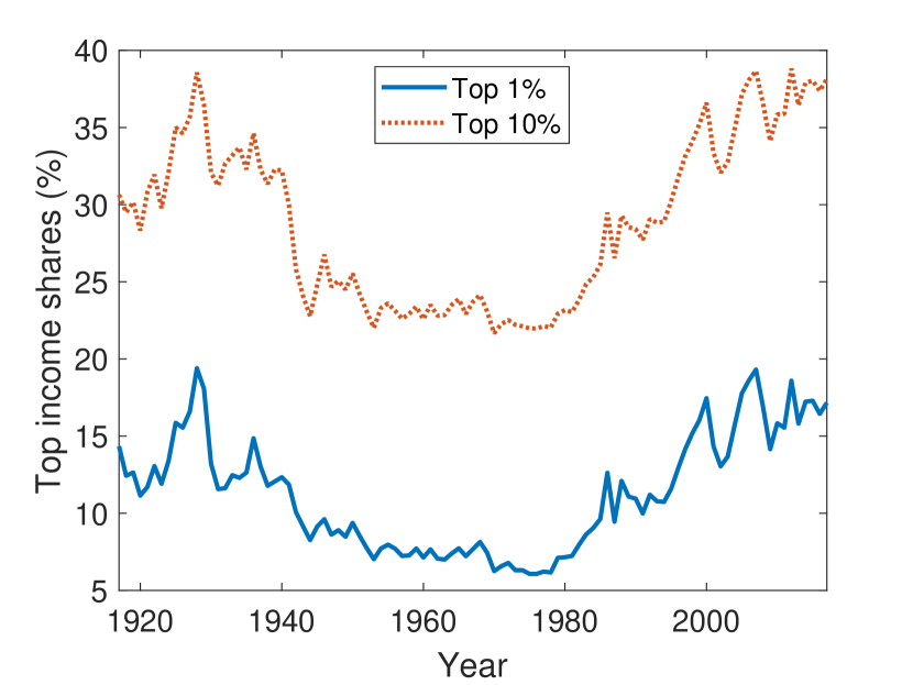
(a) Top income shares.

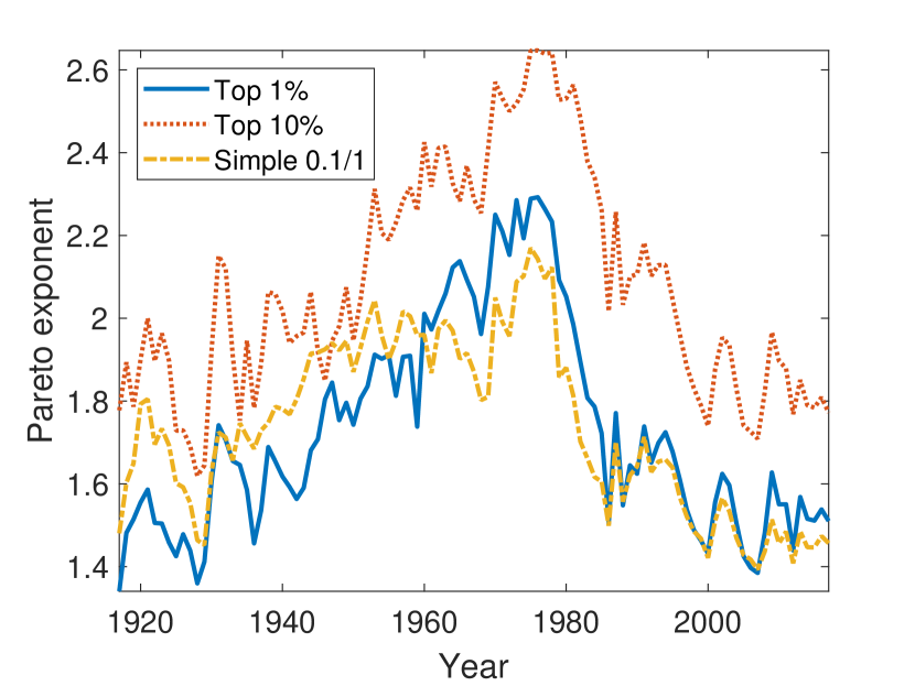
(b) Pareto exponent.

Figure 1: Income distribution in U.S.

Figure 2 repeats the analysis for France. Again, the point estimates of the Pareto exponent when using the top 1% and 10% groups differ significantly, and therefore we should focus on the 1% result. Unlike in U.S., where 1960–1980 appears to be an unusual period of low inequality (high Pareto exponent), in France the Pareto exponent is relatively stable at around 1.5 prewar and 2 postwar. Therefore there seems to be a regime change at around World War II, corroborating to Piketty (2003)’s analysis.

(a) Top income shares.

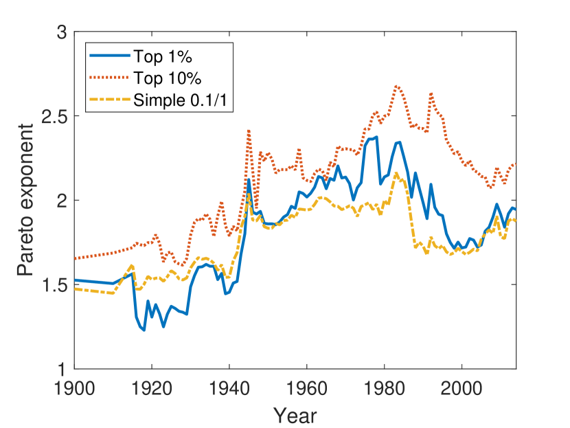
(b) Pareto exponent.

Figure 2: Income distribution in France.

Conducting statistical inference on $\alpha$ typically requires the sample size $n$ if the dataset is cross-sectional. In our dataset, which consists only of the top income shares, the sample size is unknown. However, there are potentially two approaches to conduct statistical inference. One is to assume a conservative number for the sample size, and the other is to exploit the panel data structure to construct the confidence interval without the knowledge of $n$ by using the method proposed by Ibragimov and Müller (2010, 2016) and Ibragimov et al. (2015, Section 3.3).

With the first approach, it is reasonable to assume that the number of households is at least one million ($n=10^{6}$) for both U.S. and France. We can use this number to construct conservative confidence intervals as discussed in Section 3.2. Figure 3 shows the length of these conservative 95% confidence intervals, which are constructed using the asymptotic normality of $\widehat{\alpha}$ as in Corollary 3.5. For both U.S. and France, the case when using only the income shares within the top 1% (which is more relevant due to possible model misspecification), the length is at most around 0.1, which is similar to the number in Table 3 with sample size $n=10^{6}$. Therefore the confidence intervals are within $\pm 0.05$ of the estimated Pareto exponents. For example, from Figures 1(b), 2(b), and 3, we can conclude that the income Pareto exponent has significantly declined from late 1970s to early 2000s both in U.S. and France, although in U.S. the Pareto exponent has been stable at around 1.5 since 1985. Returning to the optimal taxation problem discussed in the introduction, this estimate together with income elasticity 0.3 suggests that the revenue-maximizing income tax rate is $1/(1+1.5\times 0.3)=69\%$.

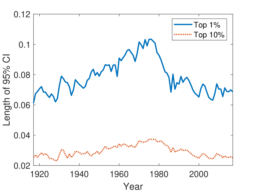
(a) U.S.

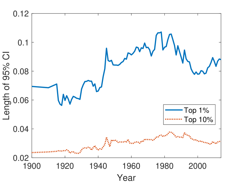
(b) France.

Figure 3: Length of conservative 95% confidence intervals of Pareto exponents.

With the second approach, consider $\left\{{\widehat{\alpha}_{1},\dots,\widehat{\alpha}_{L}}\right\}$ as $L$ estimators of $\alpha$ using $L$ independent samples, where the sample sizes can be heterogeneous. Suppose the estimators satisfy asymptotic normality such that for all $l=1,\dots,L$, we have

$$\sqrt{n_{l}}(\widehat{\alpha}_{l}-\alpha)\xrightarrow{\mathrm{d}}N(0,\sigma_{l}^{2})$$

as $n_{l}\to\infty$, where $n_{l}$ denotes the sample size of the $l$-th sample. The usual $t$-statistic for the hypothesis testing problem that

$$H_{0}:\alpha=\alpha_{0}\quad\text{against}\quad H_{1}:\alpha\neq\alpha_{0}$$

is given by $t=\sqrt{L}(\bar{\alpha}-\alpha_{0})/s_{\alpha}$, where

$$\bar{\alpha}=\frac{1}{L}\sum_{l=1}^{L}\widehat{\alpha}_{l}\quad\text{and}\quad s_{\alpha}^{2}=\frac{1}{L-1}\sum_{l=1}^{L}(\widehat{\alpha}_{l}-\bar{\alpha})^{2}.$$

We reject the null hypothesis if $\left\lvert t\right\rvert$ is larger than some critical value.

If $\sigma_{l}=\sigma$ for all $l$, the critical value is approximated by the quantile of the Student-$t$ distribution with $L-1$ degrees of freedom. If $\sigma_{l}$ is not homogeneous, Theorem 1 in Ibragimov and Müller (2010) (which is due to Bakirov and Székely (2006)) establishes that the above $t$-test with the same critical values based on the Student-$t$ distribution is still valid but conservative. More precisely, as long as the significant level $v$ is less than $0.08$ and $L\geq 2$, we have

$$\lim_{n\to\infty}P(\left\lvert t\right\rvert>F^{-1}_{t,L-1}(v/2)\mid H_{0})\leq v,$$

where $F^{-1}_{t,L-1}(v/2)$ denotes the $1-v/2$ quantile of the Student-$t$ distribution with $L-1$ degrees of freedom. Thus, an asymptotically conservative confidence interval is obtained as

$$\bar{\alpha}\pm\frac{s_{\alpha}}{\sqrt{L}}F^{-1}_{t,L-1}(v/2).$$ (4.1)

This confidence interval covers the true $\alpha$ with at least $1-v$ probability asymptotically.

Based on the previous result, we can construct the confidence intervals for $\alpha$ using the estimates from different years, which are approximately independent if the dataset for each of them are sufficiently far apart. In particular, we use the CMD estimators and the simple estimators based on (3.2) from every ten years using postwar top income share data. For example, we construct the confidence interval (4.1) for years that have identical last digit. Table 2 presents the (conservative) 95% confidence intervals of the Pareto exponent using (4.1). Because the length of confidence intervals in Table 2 is around 0.5, using a conservative estimate of sample size as in Figure 3 gives shorter confidence intervals. Besides, our short confidence intervals substantially refine the existing results about the Pareto exponent of income.

Table 2: Conservative 95% confidence intervals of Pareto exponents.

	U.S.		France
Year	CMD 1%	Simple 0.1/1	CMD 1%	Simple 0.1/1
XXX0	$(1.53,2.09)$	$(1.64,1.88)$	$(1.83,2.11)$	$(1.74,1.96)$
XXX1	$(1.61,2.05)$	$(1.61,1.88)$	$(1.80,2.09)$	$(1.71,1.96)$
XXX2	$(1.57,2.03)$	$(1.62,1.92)$	$(1.85,2.15)$	$(1.77,2.00)$
XXX3	$(1.61,2.09)$	$(1.60,1.92)$	$(1.84,2.19)$	$(1.75,2.04)$
XXX4	$(1.57,2.07)$	$(1.56,1.90)$	$(1.82,2.19)$	$(1.75,2.03)$
XXX5	$(1.52,2.11)$	$(1.54,1.89)$	$(1.80,2.27)$	$(1.76,2.07)$
XXX6	$(1.50,2.01)$	$(1.54,1.87)$	$(1.83,2.21)$	$(1.79,2.01)$
XXX7	$(1.53,2.03)$	$(1.54,1.89)$	$(1.81,2.18)$	$(1.78,1.95)$
XXX8	$(1.51,2.03)$	$(1.57,1.84)$	$(1.84,2.25)$	$(1.75,1.97)$
XXX9	$(1.56,1.99)$	$(1.60,1.90)$	$(1.86,2.12)$	$(1.77,1.94)$

Note: “Year XXX$d$” denotes the years with last digit $d$, e.g., $\left\{{1946,1956,\dots,2016}\right\}$ if $d=6$. Other entries are the $95\%$ confidence intervals of the Pareto exponent using (4.1). The left columns are based on the CMD estimator with top 1% shares, and the right columns are based on the simple estimator (3.2). See the main text for details of the two estimators.

How should a researcher choose between the two inference approaches? We generally recommend the CMD approach based on (3.6) if the sample size $n$ is observed or at least known to be larger than some threshold, say $10^{6}$. Since this approach uses cross-sectional data, we can conduct inference for $\alpha$ in each year. If $n$ is completely unknown, the method by Ibragimov and Müller (2010, 2016) is the only viable alternative. Note that this method essentially requires a panel data, where we use the cross-sectional data to construct $\widehat{\alpha}_{l}$ in the $l$-th year and then implement the $t$-test using these estimates. In our situation, these two approaches are based on different data and hence their results are not directly comparable. In particular, the approach of Ibragimov and Müller (2010, 2016) serves as a robustness check, which leads to substantially longer confidence intervals since it relies on the estimates in only 10 years. Furthermore, this method requires the constancy of the Pareto exponent $\alpha$, which is questionable as seen in Figures 1(b) and 2(b).

5 Conclusion

This paper develops an efficient minimum distance estimator of the Pareto exponent when only top income shares data are available. This is especially relevant in studying income inequality since individual level data for the top rich people are usually unavailable due to confidentiality concerns. Our estimator is consistent and asymptotically normal, and performs excellently in finite samples as shown by Monte Carlo simulations. In particular, we recommend using only top 1 instead of 10 percentile shares to study the tail of the income distribution. We estimate the Pareto exponent to be around 1.5 and stable since 1985 in U.S., and is around 1.5 and 2 before and after WWII in France.

Appendix A Proofs

Proof of Lemma 2.2.

Using (2.2a), (2.3b), and the change of variable $v=1-x$, we obtain

$$\mu(J,F) =\int_{0}^{1}J(x)F^{-1}(x)\mathop{}\!\mathrm{d}x=\int_{1-q}^{1-p}c(1-x)^{-1/\alpha}\mathop{}\!\mathrm{d}x$$

$$=\int_{p}^{q}cv^{-\xi}\mathop{}\!\mathrm{d}v=c\frac{q^{1-\xi}-p^{1-\xi}}{1-\xi},$$

which is (2.4a). To prove (2.4b), using symmetry, (2.2b), (2.3c), and the change of variable $v_{i}=1-x_{i}$, we obtain

$$\sigma^{2}(J,F)$$

$$=2\int_{0\leq x_{1}\leq x_{2}\leq 1}\frac{J(x_{1})J(x_{2})}{f(F^{-1}(x_{1}))f(F^{-1}(x_{2}))}(\min\left\{{x_{1},x_{2}}\right\}-x_{1}x_{2})\mathop{}\!\mathrm{d}x_{1}\mathop{}\!\mathrm{d}x_{2}$$

$$=2\int_{0\leq x_{1}\leq x_{2}\leq 1}\frac{J(x_{1})J(x_{2})}{f(F^{-1}(x_{1}))f(F^{-1}(x_{2}))}x_{1}(1-x_{2})\mathop{}\!\mathrm{d}x_{1}\mathop{}\!\mathrm{d}x_{2}$$

$$=\frac{2c^{2}}{\alpha^{2}}\int_{p\leq v_{2}\leq v_{1}\leq q}\frac{1}{v_{1}^{1+1/\alpha}v_{2}^{1+1/\alpha}}(1-v_{1})v_{2}\mathop{}\!\mathrm{d}v_{1}\mathop{}\!\mathrm{d}v_{2}$$

$$=2c^{2}\xi^{2}\int_{p}^{q}\int_{p}^{v_{1}}\frac{1-v_{1}}{v_{1}^{1+\xi}}v_{2}^{-\xi}\mathop{}\!\mathrm{d}v_{2}\mathop{}\!\mathrm{d}v_{1}$$

$$=\frac{2c^{2}\xi^{2}}{1-\xi}\int_{p}^{q}\frac{1-v_{1}}{v_{1}^{1+\xi}}(v_{1}^{1-\xi}-p^{1-\xi})\mathop{}\!\mathrm{d}v_{1}$$

$$=\frac{2c^{2}\xi^{2}}{1-\xi}\int_{p}^{q}(v^{-2\xi}-v^{1-2\xi}-p^{1-\xi}v^{-1-\xi}+p^{1-\xi}v^{-\xi})\mathop{}\!\mathrm{d}v$$

$$=\frac{2c^{2}\xi^{2}}{1-\xi}\left(\frac{q^{1-2\xi}-p^{1-2\xi}}{1-2\xi}-\frac{q^{2-2\xi}-p^{2-2\xi}}{2-2\xi}+p^{1-\xi}\frac{q^{-\xi}-p^{-\xi}}{\xi}+p^{1-\xi}\frac{q^{1-\xi}-p^{1-\xi}}{1-\xi}\right)$$

$$=\frac{2c^{2}\xi^{2}}{1-\xi}\left(\frac{q^{1-2\xi}-p^{1-2\xi}}{1-2\xi}+p^{1-\xi}\frac{q^{-\xi}-p^{-\xi}}{\xi}+\frac{2p^{1-\xi}q^{1-\xi}-p^{2-2\xi}-q^{2-2\xi}}{2-2\xi}\right),$$

where $\frac{q^{1-2\xi}-p^{1-2\xi}}{1-2\xi}=\log\frac{q}{p}$ if $\xi=1/2$. ∎

Proof of Lemma 2.3.

The formula for $\Sigma_{kk}$ follows from Lemma 2.2. Suppose $j<k$ and let $v$ be the asymptotic variance of $\bar{Y}_{j}+\bar{Y}_{k}$. On the one hand, we have

$$v=\sigma_{j}^{2}+\sigma_{k}^{2}+2\Sigma_{jk}.$$

On the other hand, noting that $\bar{Y}_{j}+\bar{Y}_{k}$ is asymptotically equivalent as $L_{n}$ in Lemma 2.1 with

$$J(x)=1[1-p_{j+1}<x\leq 1-p_{j}]+1[1-p_{k+1}<x\leq 1-p_{k}],$$

it follows from the proof of Lemma 2.2 that

$$v=I_{jj}+I_{jk}+I_{kj}+I_{kk},$$

where

$$I_{jk}=c^{2}\xi^{2}\int_{p_{j}}^{p_{j+1}}\int_{p_{k}}^{p_{k+1}}\frac{1}{v_{1}^{1+\xi}v_{2}^{1+\xi}}(\min\left\{{1-v_{1},1-v_{2}}\right\}-(1-v_{1})(1-v_{2}))\mathop{}\!\mathrm{d}v_{1}\mathop{}\!\mathrm{d}v_{2}.$$ (A.1)

Clearly we have $I_{jj}=\sigma_{j}^{2}$ and $I_{kk}=\sigma_{k}^{2}$. By Fubini’s theorem, $I_{jk}=I_{kj}$. Therefore $\Sigma_{jk}=I_{jk}$. Since $j<k$ and hence $p_{j}<p_{k}$, we obtain

$$\Sigma_{jk} =c^{2}\xi^{2}\int_{p_{j}}^{p_{j+1}}\int_{p_{k}}^{p_{k+1}}\frac{1}{v_{1}^{1+\xi}v_{2}^{1+\xi}}(1-v_{1})v_{2}\mathop{}\!\mathrm{d}v_{1}\mathop{}\!\mathrm{d}v_{2}$$

$$=c^{2}\xi^{2}\left(\int_{p_{j}}^{p_{j+1}}v_{2}^{-\xi}\mathop{}\!\mathrm{d}v_{2}\right)\left(\int_{p_{k}}^{p_{k+1}}(v_{1}^{-1-\xi}-v_{1}^{-\xi})\mathop{}\!\mathrm{d}v_{1}\right)$$

$$=c^{2}\xi^{2}\frac{p_{j+1}^{1-\xi}-p_{j}^{1-\xi}}{1-\xi}\left(-\frac{p_{k+1}^{-\xi}-p_{k}^{-\xi}}{\xi}-\frac{p_{k+1}^{1-\xi}-p_{k}^{1-\xi}}{1-\xi}\right)$$

$$=-c^{2}\xi^{2}\frac{p_{j+1}^{1-\xi}-p_{j}^{1-\xi}}{1-\xi}\left(\frac{p_{k+1}^{-\xi}-p_{k}^{-\xi}}{\xi}+\frac{p_{k+1}^{1-\xi}-p_{k}^{1-\xi}}{1-\xi}\right),$$

which is (2.4b).

To show that $\Sigma$ is positive definite, noting that $\Sigma_{jk}=I_{jk}=I_{kj}$ and (A.1) holds, we have

$$\Sigma_{jk}=\int_{[p_{1},1]^{2}}\phi_{j}(v_{1})\phi_{k}(v_{2})\frac{\min\left\{{1-v_{1},1-v_{2}}\right\}-(1-v_{1})(1-v_{2})}{v_{1}v_{2}}\mathop{}\!\mathrm{d}v_{1}\mathop{}\!\mathrm{d}v_{2},$$

where $\phi_{j}(v)=c\xi v^{-\xi}1[p_{j}\leq v<p_{j+1}]$. Take any vector $z=(z_{1},\dots,z_{K})^{\top}\in\mathbb{R}^{K}$. Then as in the proof of Lemma 2.2, we obtain

$$z^{\top}\Sigma z =2\sum_{j,k}z_{j}z_{k}\int_{p_{1}\leq v_{2}\leq v_{1}\leq 1}\phi_{j}(v_{1})\phi_{k}(v_{2})\frac{1-v_{1}}{v_{1}}\mathop{}\!\mathrm{d}v_{1}\mathop{}\!\mathrm{d}v_{2}$$

$$=2\sum_{j,k}z_{j}z_{k}\int_{p_{1}}^{1}\int_{p_{1}}^{v_{1}}\phi_{j}(v_{1})\phi_{k}(v_{2})\frac{1-v_{1}}{v_{1}}\mathop{}\!\mathrm{d}v_{2}\mathop{}\!\mathrm{d}v_{1}$$

$$=2\int_{p_{1}}^{1}\int_{p_{1}}^{v_{1}}\phi(v_{1})\phi(v_{2})\frac{1-v_{1}}{v_{1}}\mathop{}\!\mathrm{d}v_{2}\mathop{}\!\mathrm{d}v_{1},$$

where $\phi(v)=\sum_{k=1}^{K}z_{k}\phi_{k}(v)$. Since $\phi$ is piece-wise continuous, we can take an absolutely continuous primitive function $\Phi=\int\phi$ such that $\Phi(p_{1})=0$. By the fundamental theorem of calculus, we obtain

$$z^{\top}\Sigma z=2\int_{p_{1}}^{1}\phi(v)\Phi(v)\frac{1-v}{v}\mathop{}\!\mathrm{d}v.$$

Let $I$ be the integral ignoring the factor 2. Using integration by parts, we obtain

$$I =\int_{p_{1}}^{1}\phi(v)\Phi(v)\frac{1-v}{v}\mathop{}\!\mathrm{d}v=\int_{p_{1}}^{1}\Phi^{\prime}(v)\Phi(v)\frac{1-v}{v}\mathop{}\!\mathrm{d}v$$

$$=\left[\Phi(v)^{2}\frac{1-v}{v}\right]_{p_{1}}^{1}-\int_{p_{1}}^{1}\Phi(v)\left(\Phi^{\prime}(v)\frac{1-v}{v}-\frac{\Phi(v)}{v^{2}}\right)\mathop{}\!\mathrm{d}v$$

$$=-I+\int_{p_{1}}^{1}\frac{\Phi(v)^{2}}{v^{2}}\mathop{}\!\mathrm{d}v$$

$$\iff z^{\top}\Sigma z=2I=\int_{p_{1}}^{1}\frac{\Phi(v)^{2}}{v^{2}}\mathop{}\!\mathrm{d}v\geq 0,$$

so $\Sigma$ is positive semidefinite. Since $\Phi$ is continuous, equality holds if and only if $\Phi\equiv 0\iff z=0$. Therefore $\Sigma$ is positive definite. ∎

Proof of Proposition 3.1.

Let $Z=(Z_{1},\dots,Z_{K})^{\top}\sim N(0,\Sigma)$. Since $\bar{Y}_{k}\xrightarrow{\mathrm{p}}\mu_{k}$ and $\sqrt{n}(\bar{Y}_{k}-\mu_{k})\xrightarrow{\mathrm{d}}Z_{k}$ by (2.6), using the definition of $S_{k}$, $R_{k}$, and $\bar{Y}_{k}$, we obtain

$$\sqrt{n}(\bar{s}_{k}-r_{k}) =\sqrt{n}\left(\frac{S_{k+1}-S_{k}}{S_{K+1}-S_{K}}-\frac{\mu_{k}}{\mu_{K}}\right)=\sqrt{n}\left(\frac{n\bar{Y}_{k}/\sum Y_{i}}{n\bar{Y}_{K}/\sum Y_{i}}-\frac{\mu_{k}}{\mu_{K}}\right)$$

$$=\sqrt{n}\left(\frac{\bar{Y}_{k}}{\bar{Y}_{K}}-\frac{\mu_{k}}{\mu_{K}}\right)=\frac{1}{\bar{Y}_{K}}\sqrt{n}(\bar{Y}_{k}-\mu_{k})-\frac{\mu_{k}}{\mu_{K}\bar{Y}_{K}}\sqrt{n}(\bar{Y}_{K}-\mu_{K})$$

$$\xrightarrow{\mathrm{d}}\frac{1}{\mu_{K}}Z_{k}-\frac{\mu_{k}}{\mu_{K}^{2}}Z_{K}.$$

Expressing this in matrix form, we obtain

$$\sqrt{n}(\bar{s}-r)\xrightarrow{\mathrm{d}}HZ\sim N(0,H\Sigma H^{\top}).$$

Since by Lemma 2.2 each $\mu_{k}$ is proportional to $c$ and each element of $\Sigma$ is proportional to $c^{2}$, the vector $r$ and matrix $\Omega=H\Sigma H^{\top}$ depend only on $\alpha$. Since $\Sigma$ is positive definite by Lemma 2.3 and $H$ has full row rank, $\Omega$ is also positive definite. ∎

Proof of Proposition 3.2.

We prove the contrapositive. Let $\xi=1/\alpha$ and $\xi_{0}=1/\alpha_{0}$. If $r(\alpha)=r(\alpha_{0})$, using $r_{k}=\mu_{k}/\mu_{K}$ and (2.4a), in particular

$$r_{K-1}(\alpha)=r_{K-1}(\alpha_{0}) \iff\frac{p_{K}^{1-\xi}-p_{K-1}^{1-\xi}}{p_{K+1}^{1-\xi}-p_{K}^{1-\xi}}=\frac{p_{K}^{1-\xi_{0}}-p_{K-1}^{1-\xi_{0}}}{p_{K+1}^{1-\xi_{0}}-p_{K}^{1-\xi_{0}}}$$

$$\iff\frac{1-a^{1-\xi}}{b^{1-\xi}-1}=\frac{1-a^{1-\xi_{0}}}{b^{1-\xi_{0}}-1},$$

where $a=p_{K-1}/p_{K}<1$ and $b=p_{K+1}/p_{K}>1$. By Lemma A.1 below, the left-hand side is monotone in $\xi\in(0,1)$. Therefore $\xi=\xi_{0}$ and hence $\alpha=\alpha_{0}$. ∎

Lemma A.1.

Let $a,b>0$, $a,b\neq 1$, and $a\neq b$. Then $f(x)=\frac{a^{x}-1}{b^{x}-1}$ is either strictly increasing or decreasing in $x>0$.

Proof.

By simple algebra, we obtain

$$f^{\prime}(x)=\frac{a^{x}\log a(b^{x}-1)-b^{x}\log b(a^{x}-1)}{(b^{x}-1)^{2}}=\frac{b^{x}\log b}{b^{x}-1}\left(\frac{a^{x}\log a}{b^{x}\log b}-\frac{a^{x}-1}{b^{x}-1}\right).$$

Applying Cauchy’s mean value theorem to $g_{1}(x)=a^{x}$ and $g_{2}(x)=b^{x}$, there exists $0<y<x$ such that

$$\frac{a^{x}-1}{b^{x}-1}=\frac{g_{1}(x)-g_{1}(0)}{g_{2}(x)-g_{2}(0)}=\frac{g_{1}^{\prime}(y)}{g_{2}^{\prime}(y)}=\frac{a^{y}\log a}{b^{y}\log b}.$$

Therefore

$$f^{\prime}(x)=\frac{b^{x}\log b}{b^{x}-1}\left(\frac{a^{x}\log a}{b^{x}\log b}-\frac{a^{y}\log a}{b^{y}\log b}\right)=\frac{b^{x}\log a}{b^{x}-1}\left(\left(\frac{a}{b}\right)^{x}-\left(\frac{a}{b}\right)^{y}\right).$$

Since $a,b>0$, $a,b\neq 1$, $a\neq b$, and $0<y<x$, the sign of $\log a$ depends on $a\gtrless 1$, the sign of $b^{x}-1$ depends on $b\gtrless 1$, and the sign of $(a/b)^{x}-(a/b)^{y}$ depends on $a\gtrless b$. Therefore $f^{\prime}(x)$ has a constant sign. ∎

Appendix B Simulation

In this appendix we evaluate the finite sample properties of the continuously updated minimum distance estimator (3.5) through simulations.

B.1 Simulation design

We consider three data generating processes (DGPs), (i) Pareto distribution, (ii) absolute value of the Student-$t$ distribution, and (iii) double Pareto-lognormal distribution (dPlN). For the Pareto distribution, we set the Pareto exponent to $\alpha=2$ and (without loss of generality) the minimum size to $c=1$. For the Student-$t$ distribution, we set the degree of freedom to $\nu=2$ so that the Pareto exponent is 2. The double Pareto-lognormal distribution is the product of independent double Pareto (Reed, 2001) and lognormal variables. dPlN has been documented to fit well to size distributions of economic variables including income (Reed, 2003), city size (Giesen et al., 2010), and consumption (Toda, 2017). Reed and Jorgensen (2004) show that a dPlN variable $Y$ can be generated as

$$Y=\exp(\mu+\sigma X_{1}+X_{2}/\alpha-X_{3}/\beta),$$

where $X_{1},X_{2},X_{3}$ are independent and $X_{1}\sim N(0,1)$ and $X_{2},X_{3}\sim\mathrm{Exp}(1)$. For parameter values, we set $\mu=0$, $\sigma=0.5$, $\alpha=2$, and $\beta=1$, which are typical values for income data as documented in Toda (2012).

The simulation design is as follows. For each DGP, we generate i.i.d. samples with size $n=10^{4},10^{5},10^{6}$. We set the top percentiles as in (3.1), which are the numbers reported in Piketty and Saez (2003). Because the distribution is not exactly Pareto for DGP 2 (Student-$t$) and 3 (dPlN), we expect that the estimation suffers from model misspecification when we use large top income percentile such as 10% ($p_{6}=0.1$). Therefore to evaluate the robustness against model misspecification, we also consider using only the top 5% group ($p_{1}$–$p_{5}$) and the top 1% group ($p_{1}$–$p_{4}$). Thus, in total there are $3^{3}=27$ specifications (three DGPs, three sample sizes, and three choices of top income percentiles). For each specification, we estimate $\widehat{\alpha}$, construct the confidence interval based on inverting the likelihood ratio test in Proposition 3.6, and implement the specification test in Proposition 3.7 using the algorithm in Section 3.2. The numbers are based on $M=\text{1,000}$ simulations. Table 3 shows the simulation results.

Table 3: Finite sample properties of continuously updated minimum distance estimator.

DGP	Pareto			$\left\lvert t\right\rvert$			dPlN
Top%	10%	5%	1%	10%	5%	1%	10%	5%	1%
$n$	Bias
$10^{4}$	-0.02	-0.03	-0.04	-0.13	-0.07	-0.06	-0.05	-0.03	-0.04
$10^{5}$	0.00	0.00	0.00	-0.12	-0.04	-0.02	-0.04	-0.01	-0.01
$10^{6}$	0.00	0.00	0.00	-0.11	-0.04	-0.01	-0.04	0.00	0.00
$n$	RMSE
$10^{4}$	0.08	0.13	0.24	0.15	0.15	0.25	0.09	0.13	0.24
$10^{5}$	0.02	0.04	0.07	0.12	0.06	0.07	0.04	0.04	0.07
$10^{6}$	0.01	0.01	0.02	0.11	0.04	0.03	0.04	0.01	0.02
$n$	Coverage
$10^{4}$	0.92	0.92	0.92	0.50	0.86	0.90	0.85	0.91	0.90
$10^{5}$	0.96	0.94	0.95	0.00	0.76	0.94	0.59	0.93	0.95
$10^{6}$	0.92	0.95	0.95	0.00	0.04	0.91	0.00	0.92	0.96
$n$	Length
$10^{4}$	0.28	0.48	0.96	0.27	0.47	0.95	0.28	0.48	0.96
$10^{5}$	0.09	0.15	0.29	0.09	0.15	0.29	0.09	0.15	0.29
$10^{6}$	0.03	0.05	0.09	0.03	0.05	0.09	0.03	0.05	0.09
$n$	Rejection probability
$10^{4}$	0.04	0.02	0.01	0.02	0.02	0.01	0.03	0.03	0.01
$10^{5}$	0.02	0.01	0.01	0.29	0.02	0.01	0.04	0.01	0.01
$10^{6}$	0.02	0.02	0.02	1.00	0.13	0.02	0.66	0.01	0.01

Note: Each data genrating process (DGP) has Pareto exponent $\alpha=2$. $\left\lvert t\right\rvert$: absolute value of the Student-$t$ distribution. dPlN: double Pareto-lognormal distribution. $n$: sample size. Bias: $\frac{1}{M}\sum_{m=1}^{M}(\widehat{\alpha}_{m}-\alpha)$, where $m$ indexes simulations and $M=\text{1,000}$. RMSE: root mean squared error defined by $\sqrt{\frac{1}{M}\sum_{m=1}^{M}(\widehat{\alpha}_{m}-\alpha)^{2}}$. “Coverage” is the fraction of simulations for which the true value $\alpha=2$ falls into the 95% confidence interval. “Length” is the average length of confidence intervals across simulations. “Rejection probability” is the fraction of simulations for which the specification test in Proposition 3.7 rejects.

We can make a few observations from Table 3. First, when the model is correctly specified (Pareto), the finite sample properties are excellent. In particular, the coverage rate is close to the nominal value 0.95. In this case, using more top percentiles (including the top 10%) is more efficient (has smaller bias and RMSE) because it exploits more information. Second, when the model is misspecified (Student-$t$ or dPlN distributions), including large top percentiles (10%) leads to large bias and incorrect coverage. Thus, it is preferable to use only percentiles within the top 1% or 5% for robustness against potential model misspecification. This is seen from the rejection probability of the specification test. Third, when the sample size is large ($n=10^{6}$, which is typical for administrative data) and we use the top 1% group, the finite sample properties are good for all distributions considered here.

Because our estimation method is based on asymptotic normality, one may be concerned whether it is a good approximation in finite samples. To address this issue, Figure 4 plots the kernel densities of $\widehat{\alpha}$ (normalized by subtracting the true value $\alpha=2$ and dividing by the sample standard deviation) based on $M=\text{1,000}$ simulations. Each figure shows the results for three sample sizes ($n=10^{4},10^{5},10^{6}$) as well as the standard normal density. Under the Pareto DGP, the distribution of $\widehat{\alpha}$ is very well approximated by the standard normal. Under the other two DGPs, however, when we use the top 10% shares the distribution of $\widehat{\alpha}$ is centered far away from the true value due to model misspecification. This bias disappears as we include only small top percentiles (e.g., only top 0–1%), as we can see from the right panels in Figure 4.

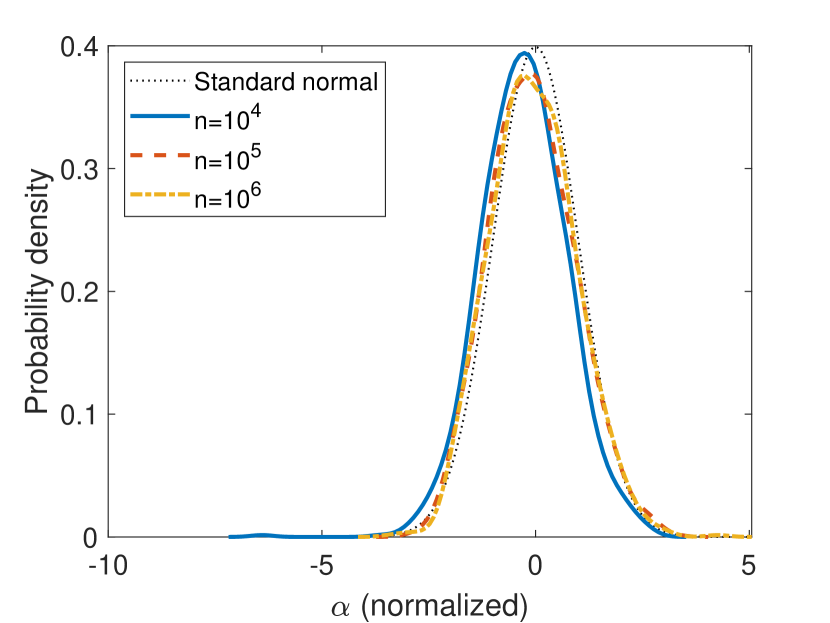
(a) Pareto, top 10%

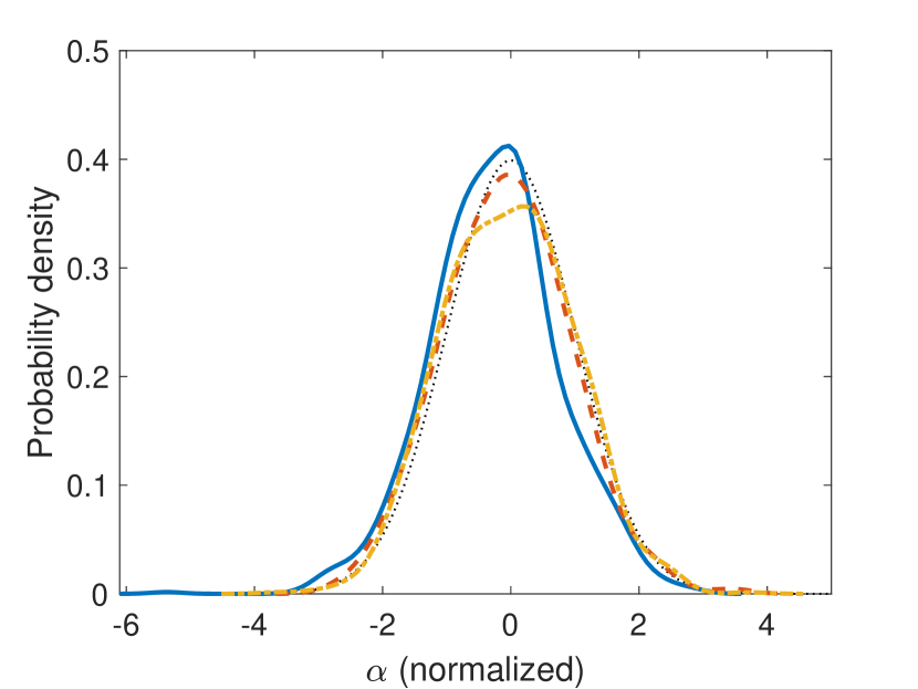
(b) Pareto, top 5%

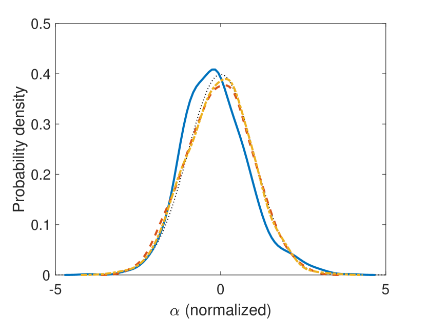
(c) Pareto, top 1%

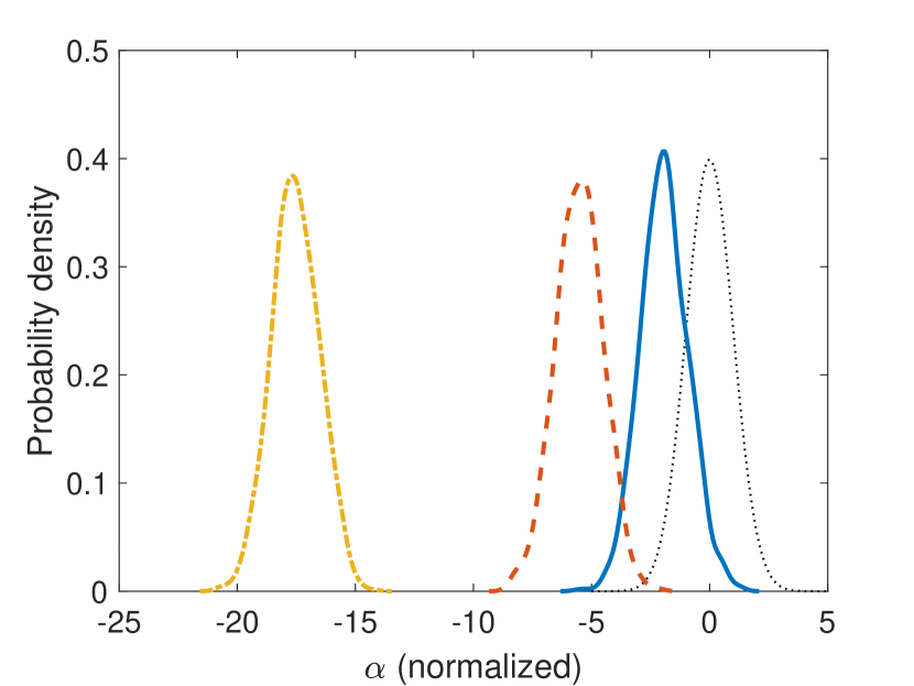
(d) $\left\lvert t\right\rvert$, top 10%

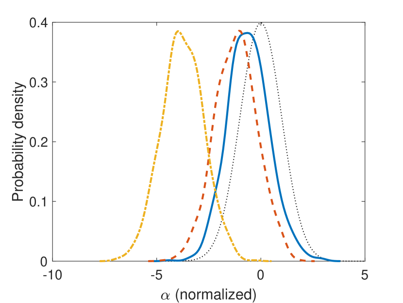
(e) $\left\lvert t\right\rvert$, top 5%

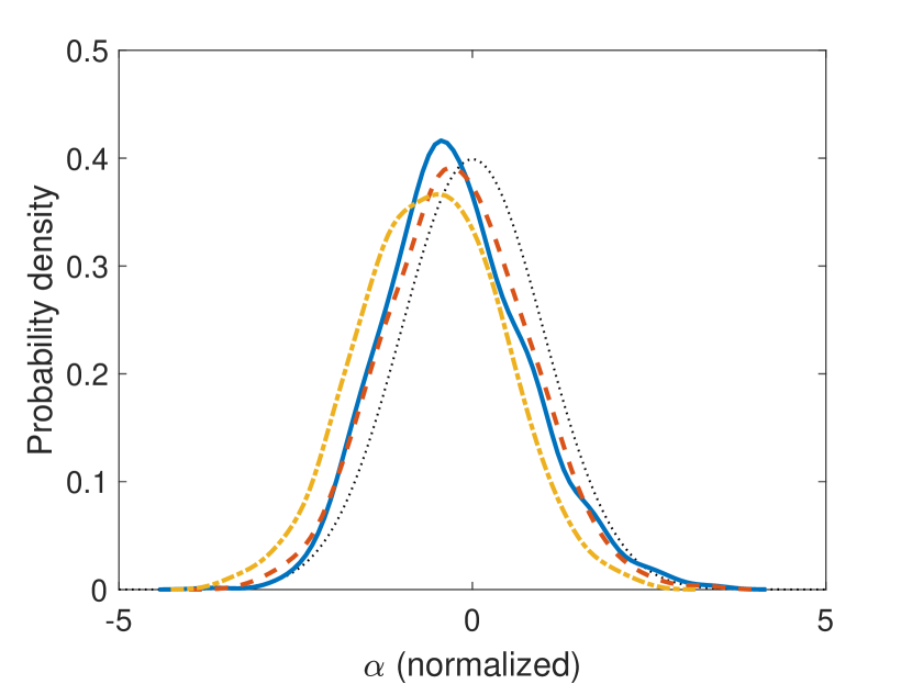
(f) $\left\lvert t\right\rvert$, top 1%

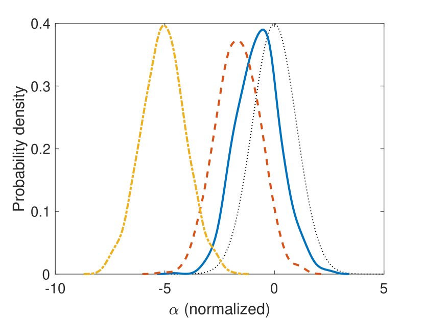
(g) dPlN, top 10%

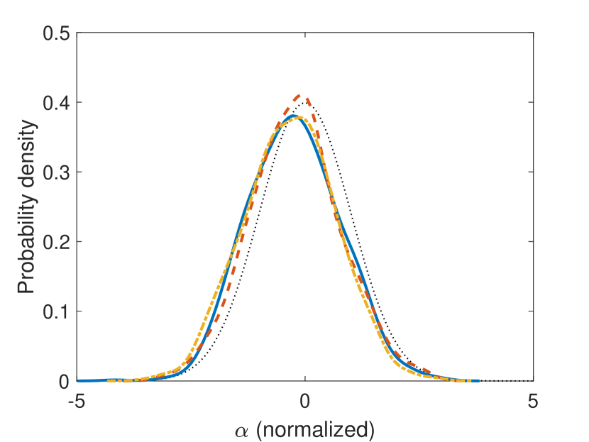
(h) dPlN, top 5%

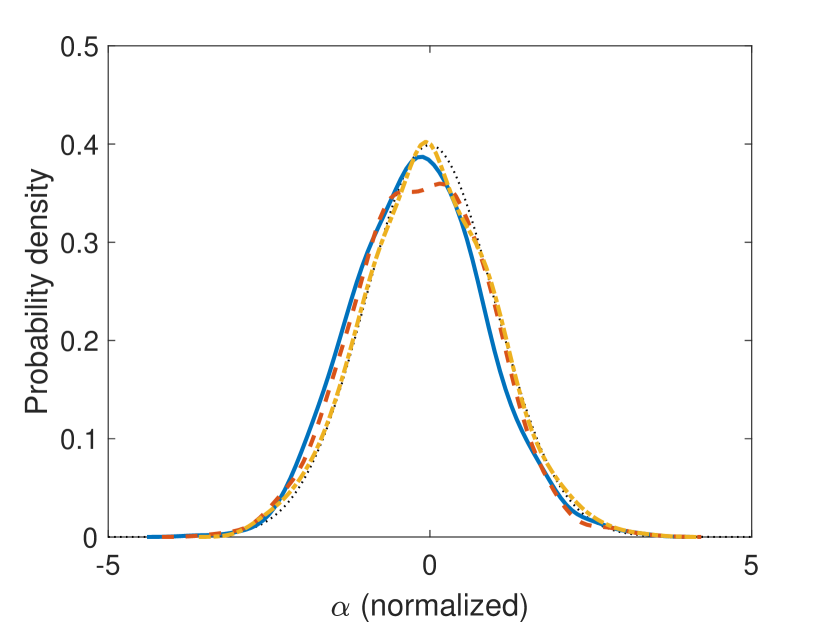
(i) dPlN, top 1%

Figure 4: Kernel density of estimated Pareto exponent $\widehat{\alpha}$.

Note: Each panel shows the kernel density of normalized $\widehat{\alpha}$ (subtracting the true value $\alpha=2$ and dividing by the sample standard deviation). See caption of Table 3 for the simulation design.

B.2 Excluding small top percentiles

Because our estimation method is based on the asymptotic distribution, one concern is that including a very small top percentile (such as $p_{1}=0.01\%$) may worsen the finite sample properties. To address this issue, we redo the simulation in Appendix B.1 but by excluding small top percentiles. Specifically, we consider using only $p_{2}$–$p_{6}$, $p_{3}$–$p_{6}$, and $p_{4}$–$p_{6}$, where the top percentiles are given by (3.1). Table 4 shows the results. Compared with Table 3 using all percentiles ($p_{1}$–$p_{6}$, columns labeled “10%”), excluding the smallest top percentiles yields similar finite sample properties in terms of bias, RMSE, coverage, and length. However, the rejection probability approaches 0 as we exclude more top percentiles, so the test loses power.

Table 4: Finite sample properties of continuously updated minimum distance estimator excluding small top shares.

DGP	Pareto			$\left\lvert t\right\rvert$			dPIN
Top%	$p_{2}$–$p_{6}$	$p_{3}$–$p_{6}$	$p_{4}$–$p_{6}$	$p_{2}$–$p_{6}$	$p_{3}$–$p_{6}$	$p_{4}$–$p_{6}$	$p_{2}$–$p_{6}$	$p_{3}$–$p_{6}$	$p_{4}$–$p_{6}$
$n$	Bias
$10^{4}$	-0.01	-0.00	0.00	-0.12	-0.12	-0.12	-0.04	-0.04	-0.04
$10^{5}$	0.00	0.00	0.00	-0.12	-0.12	-0.13	-0.04	-0.04	-0.04
$10^{6}$	0.00	0.00	0.00	-0.11	-0.12	-0.13	-0.04	-0.04	-0.04
$n$	RMSE
$10^{4}$	0.07	0.07	0.08	0.14	0.14	0.14	0.08	0.08	0.08
$10^{5}$	0.02	0.02	0.02	0.12	0.12	0.13	0.04	0.04	0.05
$10^{6}$	0.01	0.01	0.01	0.12	0.12	0.13	0.04	0.04	0.04
$n$	Coverage
$10^{4}$	0.94	0.95	0.96	0.55	0.58	0.57	0.90	0.92	0.91
$10^{5}$	0.95	0.95	0.95	0.00	0.00	0.00	0.61	0.63	0.58
$10^{6}$	0.92	0.92	0.92	0.00	0.00	0.00	0.00	0.00	0.00
$n$	Length
$10^{4}$	0.29	0.30	0.31	0.28	0.28	0.29	0.28	0.29	0.30
$10^{5}$	0.09	0.09	0.10	0.09	0.09	0.09	0.09	0.09	0.09
$10^{6}$	0.03	0.03	0.03	0.03	0.03	0.03	0.03	0.03	0.03
$n$	Rejection probability
$10^{4}$	0.01	0.01	0.00	0.02	0.02	0.00	0.01	0.01	0.00
$10^{5}$	0.02	0.02	0.00	0.34	0.33	0.00	0.06	0.06	0.00
$10^{6}$	0.02	0.02	0.00	1.00	1.00	0.00	0.67	0.67	0.00

Note: See caption of Table 3 for the simulation design.

B.3 Comparison with the simple estimator

In this appendix we compare the finite sample performance of our classical minimum distance estimator (CMD) of the Pareto exponent to the simple estimator in (3.2). For the simple estimator, we set $(p,q)=(0.1,1)/100$ as is common in the literature, and we also consider $(p,q)=(0.1,0.5)/100,(0.5,1)/100$. For the CMD estimator, to make the results comparable, we use $(p_{1},p_{2},p_{3},p_{4})=(0.01,0.1,0.5,1)/100$. Table 5 shows the results. According to the table, the CMD estimator uniformly outperforms the simple estimator in (3.2) in terms of bias and RMSE.

Table 5: Finite sample properties of continuously updated minimum distance estimator and the simple estimator in (3.2).

	Bias				RMSE
$100(p,q)$	CMD	(.1,1)	(.1,.5)	(.5,1)	CMD	(.1,1)	(.1,.5)	(.5,1)
$n$	Pareto
$10^{4}$	-0.04	0.19	0.24	0.09	0.24	0.44	0.53	0.29
$10^{5}$	0.00	0.03	0.04	0.02	0.07	0.15	0.18	0.11
$10^{6}$	0.00	0.00	0.00	0.00	0.02	0.06	0.07	0.04
$n$	$\left\lvert t\right\rvert$
$10^{4}$	-0.06	0.17	0.23	0.07	0.25	0.42	0.52	0.28
$10^{5}$	-0.02	0.03	0.04	0.01	0.07	0.16	0.18	0.11
$10^{6}$	-0.01	0.00	0.00	-0.01	0.03	0.05	0.06	0.04
$n$	dPlN
$10^{4}$	-0.04	0.19	0.25	0.10	0.24	0.43	0.53	0.27
$10^{5}$	-0.01	0.03	0.03	0.01	0.07	0.14	0.17	0.10
$10^{6}$	0.00	0.00	0.01	0.00	0.02	0.06	0.07	0.05

Note: See caption of Table 3 for the simulation design. “CMD” refers to the continuously updated minimum distance estimator with top 0.01, 0.1, 0.5, 1 percentiles. $100(p,q)$ denotes the top percentiles used in the simple estimator (3.2).

References

- Aoki and Nirei (2017) Shuhei Aoki and Makoto Nirei. Zipf’s law, Pareto’s law, and the evolution of top incomes in the United States. American Economic Journal: Macroeconomics, 9(3):36–71, July 2017. doi:10.1257/mac.20150051.
- Atkinson and Piketty (2010) Anthony B. Atkinson and Thomas Piketty, editors. Top Incomes: A Global Perspective. Oxford University Press, New York, NY, 2010.
- Auerbach (1913) Felix Auerbach. Das Gesetz der Bevölkerungskonzentration. Petermanns Geographische Mitteilungen, 59:74–76, 1913. URL http://www.mpi.nl/publications/escidoc-2271118.
- Axtell (2001) Robert L. Axtell. Zipf distribution of U.S. firm sizes. Science, 293(5536):1818–1820, September 2001. doi:10.1126/science.1062081.
- Bakirov and Székely (2006) Nail K. Bakirov and Gábor J. Székely. Student’s -test for Gaussian scale mixtures. Journal of Mathematical Sciences, 139(3):6497–6505, 2006. doi:10.1007/s10958-006-0366-5.
- Balkema and de Haan (1974) August A. Balkema and Laurens de Haan. Residual life time at great age. Annals of Probability, 2(5):792–804, 1974. doi:10.1214/aop/1176996548.
- Beach and Davidson (1983) Charles M. Beach and Russell Davidson. Distribution-free statistical inference with Lorenz curves and income shares. Review of Economic Studies, 50(4):723–735, October 1983. doi:10.2307/2297772.
- Beach and Richmond (1985) Charles M. Beach and James Richmond. Joint confidence intervals for income shares and Lorenz curves. International Economic Review, 26(2):439–450, June 1985. doi:10.2307/2526594.
- Bingham et al. (1987) Nicholas H. Bingham, Charles M. Goldie, and Jozef L. Teugels. Regular Variation, volume 27 of Encyclopedia of Mathematics and Its Applications. Cambridge University Press, 1987.
- Brzezinski (2013) Michal Brzezinski. Asymptotic and bootstrap inference for top income shares. Economics Letters, 120(1):10–13, July 2013. doi:10.1016/j.econlet.2013.03.045.
- Chen (2018) Yi-Ting Chen. A unified approach to estimating and testing income distributions with grouped data. Journal of Business and Economic Statistics, 36(3):438–455, July 2018. doi:10.1080/07350015.2016.1194762.
- Chiang (1956) Chin Long Chiang. On regular best asymptotically normal estimates. Annals of Mathematical Statistics, 27(2):336–351, June 1956. doi:10.1214/aoms/1177728262.
- Chotikapanich et al. (2007) Duangkamon Chotikapanich, William E. Griffiths, and D. S. Prasada Rao. Estimating and combining national income distributions using limited data. Journal of Business and Economic Statistics, 25(1):97–109, January 2007. doi:10.1198/073500106000000224.
- Chotikapanich et al. (2012) Duangkamon Chotikapanich, William E. Griffiths, D. S. Prasada Rao, and Vicar Valencia. Global income distributions and inequality, 1993 and 2000: Incorporating country-level inequality modeled with beta distributions. Review of Economics and Statistics, 94(1):52–73, February 2012. doi:10.1162/REST_a_00145.
- de Haan and Ferreira (2006) Laurens de Haan and Ana Ferreira. Extreme Value Theory: An Introduction. Springer Series in Operations Research and Financial Engineering. Springer, NY, 2006.
- Feenberg and Poterba (1993) Daniel R. Feenberg and James M. Poterba. Income inequality and the incomes of very high-income taxpayers: Evidence from tax returns. Tax Policy and the Economy, 7:145–177, 1993. doi:10.1086/tpe.7.20060632.
- Ferguson (1958) Thomas S. Ferguson. A method of generating best asymptotically normal estimates with application to the estimation of bacterial densities. Annals of Mathematical Statistics, 29(4):1046–1062, December 1958. doi:10.1214/aoms/1177706440.
- Gabaix (1999) Xavier Gabaix. Zipf’s law for cities: An explanation. Quarterly Journal of Economics, 114(3):739–767, August 1999. doi:10.1162/003355399556133.
- Gabaix (2009) Xavier Gabaix. Power laws in economics and finance. Annual Review of Economics, 1:255–293, 2009. doi:10.1146/annurev.economics.050708.142940.
- Gabaix and Ibragimov (2011) Xavier Gabaix and Rustam Ibragimov. Rank: A simple way to improve the OLS estimation of tail exponents. Journal of Business and Economic Statistics, 29(1):24–39, January 2011. doi:10.1198/jbes.2009.06157.
- Giesen et al. (2010) Kristian Giesen, Arndt Zimmermann, and Jens Suedekum. The size distribution across all cities—double Pareto lognormal strikes. Journal of Urban Economics, 68(2):129–137, September 2010. doi:10.1016/j.jue.2010.03.007.
- Hajargasht et al. (2012) Gholamreza Hajargasht, William E. Griffiths, Joseph Brice, D. S. Prasada Rao, and Duangkamon Chotikapanich. Inference for income distributions using grouped data. Journal of Business and Economic Statistics, 30(4):563–575, October 2012. doi:10.1080/07350015.2012.707590.
- Hill (1975) Bruce M. Hill. A simple general approach to inference about the tail of a distribution. Annals of Statistics, 3(5):1163–1174, September 1975. doi:10.1214/aos/1176343247.
- Ibragimov and Ibragimov (2018) Marat Ibragimov and Rustam Ibragimov. Heavy tails and upper-tail inequality: The case of Russia. Empirical Economics, 54(2):823–837, 2018. doi:10.1007/s00181-017-1239-0.
- Ibragimov et al. (2015) Marat Ibragimov, Rustam Ibragimov, and Johan Walden. Heavy-Tailed Distributions and Robustness in Economics and Finance. Number 214 in Lecture Notes in Statistics. Springer, 2015.
- Ibragimov and Müller (2010) Rustam Ibragimov and Ulrich K. Müller. -Statistic based correlation and heterogeneity robust inference. Journal of Business and Economic Statistics, 28(4):453–468, 2010. doi:10.1198/jbes.2009.08046.
- Ibragimov and Müller (2016) Rustam Ibragimov and Ulrich K. Müller. Inference with few heterogeneous clusters. Review of Economics and Statistics, 98(1):83–96, March 2016. doi:10.1162/REST_a_00545.
- Klass et al. (2006) Oren S. Klass, Ofer Biham, Moshe Levy, Ofer Malcai, and Sorin Solomon. The Forbes 400 and the Pareto wealth distribution. Economics Letters, 90(2):290–295, February 2006. doi:10.1016/j.econlet.2005.08.020.
- Kleiber and Kotz (2003) Christian Kleiber and Samuel Kotz. Statistical Size Distributions in Economics and Actuarial Sciences. Wiley Series in Probability and Statistics. John Wiley & Sons, Hoboken, NJ, 2003.
- Kuznets (1953) Simon Kuznets. Shares of Upper Income Groups in Income and Savings. NBER, 1953. URL https://www.nber.org/books/kuzn53-1.
- McDonald (1984) James B. McDonald. Some generalized functions for the size distribution of income. Econometrica, 52(3):647–663, May 1984. doi:10.2307/1913469.
- Müller and Wang (2017) Ulrich K. Müller and Yulong Wang. Fixed- asymptotic inference about tail properties. Journal of the American Statistical Association, 112(519):1334–1343, 2017. doi:10.1080/01621459.2016.1215990.
- Newey and McFadden (1994) Whitney K. Newey and Daniel McFadden. Large sample estimation and hypothesis testing. In Robert F. Engle and Daniel L. McFadden, editors, Handbook of Econometrics, volume 4, chapter 36, pages 2111–2245. North-Holland, Amsterdam, 1994. doi:10.1016/s1573-4412(05)80005-4.
- Pareto (1896) Vilfredo Pareto. La Courbe de la Répartition de la Richesse. Imprimerie Ch. Viret-Genton, Lausanne, 1896.
- Pareto (1897) Vilfredo Pareto. Cours d’Économie Politique, volume 2. F. Rouge, Lausanne, 1897.
- Pickands (1975) James Pickands, III. Statistical inference using extreme order statistics. Annals of Statistics, 3(1):119–131, 1975. doi:10.1214/aos/1176343003.
- Piketty (2003) Thomas Piketty. Income inequality in France, 1901–1998. Journal of Political Economy, 111(5):1004–1042, October 2003. doi:10.1086/376955.
- Piketty and Saez (2003) Thomas Piketty and Emmanuel Saez. Income inequality in the United States, 1913–1998. Quarterly Journal of Economics, 118(1):1–41, February 2003. doi:10.1162/00335530360535135.
- Piketty et al. (2014) Thomas Piketty, Emmanuel Saez, and Stefanie Stantcheva. Optimal taxation of top labor incomes: A tale of three elasticities. American Economic Journal: Economic Policy, 6(1):230–271, February 2014. doi:10.1257/pol.6.1.230.
- Reed (2001) William J. Reed. The Pareto, Zipf and other power laws. Economics Letters, 74(1):15–19, December 2001. doi:10.1016/S0165-1765(01)00524-9.
- Reed (2003) William J. Reed. The Pareto law of incomes—an explanation and an extension. Physica A, 319(1):469–486, March 2003. doi:10.1016/S0378-4371(02)01507-8.
- Reed and Jorgensen (2004) William J. Reed and Murray Jorgensen. The double Pareto-lognormal distribution—a new parametric model for size distribution. Communications in Statistics—Theory and Methods, 33(8):1733–1753, 2004. doi:10.1081/STA-120037438.
- Rozenfeld et al. (2011) Hernán D. Rozenfeld, Diego Rybski, Xavier Gabaix, and Hernán A. Makse. The area and population of cities: New insights from a different perspective on cities. American Economic Review, 101(5):2205–2225, August 2011. doi:10.1257/aer.101.5.2205.
- Saez (2001) Emmanuel Saez. Using elasticities to derive optimal income tax rates. Review of Economic Studies, 68(1):205–229, January 2001. doi:10.1111/1467-937X.00166.
- Stigler (1974) Stephen M. Stigler. Linear functions of order statistics with smooth weight functions. Annals of Statistics, 2(4):676–693, July 1974. doi:10.1214/aos/1176342756.
- Toda (2012) Alexis Akira Toda. The double power law in income distribution: Explanations and evidence. Journal of Economic Behavior and Organization, 84(1):364–381, September 2012. doi:10.1016/j.jebo.2012.04.012.
- Toda (2017) Alexis Akira Toda. A note on the size distribution of consumption: More double Pareto than lognormal. Macroeconomic Dynamics, 21(6):1508–1518, September 2017. doi:10.1017/S1365100515000942.
- Toda and Walsh (2015) Alexis Akira Toda and Kieran Walsh. The double power law in consumption and implications for testing Euler equations. Journal of Political Economy, 123(5):1177–1200, October 2015. doi:10.1086/682729.
- Toda and Wang (2019) Alexis Akira Toda and Yulong Wang. Efficient minimum distance estimation of Pareto exponent from top income shares. 2019. URL https://arxiv.org/abs/1901.02471.
- Vermeulen (2018) Philip Vermeulen. How fat is the top tail of the wealth distribution? Review of Income and Wealth, 64(2):357–387, June 2018. doi:10.1111/roiw.12279.
- Virkar and Clauset (2014) Yogesh Virkar and Aaron Clauset. Power-law distributions in binned empirical data. Annals of Applied Statistics, 8(1):89–119, 2014. doi:10.1214/13-AOAS710.
- Zipf (1949) George K. Zipf. Human Behavior and the Principle of Least Effort. Addison Wesley, Cambridge, MA, 1949.