Abstract

We introduce the bilinear bandit problem with low-rank structure in which an action takes the form of a pair of arms from two different entity types, and the reward is a bilinear function of the known feature vectors of the arms. The unknown in the problem is a $d_{1}$ by $d_{2}$ matrix $\mathbf{\Theta}^{*}$ that defines the reward, and has low rank $r\ll\min\{d_{1},d_{2}\}$. Determination of $\mathbf{\Theta}^{*}$ with this low-rank structure poses a significant challenge in finding the right exploration-exploitation tradeoff. In this work, we propose a new two-stage algorithm called “Explore-Subspace-Then-Refine” (ESTR). The first stage is an explicit subspace exploration, while the second stage is a linear bandit algorithm called “almost-low-dimensional OFUL” (LowOFUL) that exploits and further refines the estimated subspace via a regularization technique. We show that the regret of ESTR is $\widetilde{\mathcal{O}}((d_{1}+d_{2})^{3/2}\sqrt{rT})$ where $\widetilde{\mathcal{O}}$ hides logarithmic factors and $T$ is the time horizon, which improves upon the regret of $\widetilde{\mathcal{O}}(d_{1}d_{2}\sqrt{T})$ attained for a naïve linear bandit reduction. We conjecture that the regret bound of ESTR is unimprovable up to polylogarithmic factors, and our preliminary experiment shows that ESTR outperforms a naïve linear bandit reduction.

1 Introduction

Consider a drug discovery application where scientists would like to choose a (drug, protein) pair and measure whether the pair exhibits the desired interaction Luo et al. (2017). Over many repetitions of this step, one would like to maximize the number of discovered pairs with the desired interaction. Similarly, an online dating service may want to choose a (female, male) pair from the user pool, match them, and receive feedback about whether they like each other or not. For clothing websites, the recommendation system may want to choose a pair of items (top, bottom) for a customer, whose appeal depends in part on whether they match. In these applications, the two types of entities are recommended and evaluated as a unit. Having feature vectors of the entities available, the system must explore and learn what features of the two entities jointly predict positive feedback in order to make effective recommendations.

The recommendation system aims to obtain large rewards (the amount of positive feedback) but does not know ahead of time the relationship between the features and the feedback. The system thus faces two conflicting goals: choosing pairs that $(i)$ maximally help estimate the relationship (“exploration”) but which may give small rewards and $(ii)$ return relatively large, but possibly suboptimal, rewards (“exploitation”), given the limited information obtained from the feedback collected so far. Such an exploration-exploitation dilemma can be formulated as a multi-armed bandit problem Lai & Robbins (1985); Auer et al. (2002). When the feature vectors are available for each arm, one can postulate simple reward structures such as (generalized) linear models to allow a large or even infinite number of arms Auer (2002); Dani et al. (2008); Abbasi-Yadkori et al. (2011); Filippi et al. (2010), a paradigm that has received much attention during the past decade, with such applications as online news recommendations Li et al. (2010). Less is known for the situation we consider here, in which the recommendation (action) involves two different entity types and forms a bilinear structure. The closest work we are aware of is Kveton et al. (2017) whose action structure is the same as ours but without arm feature vectors. Factored bandits Zimmert & Seldin (2018) provide a more general view with $L$ entity types rather than two, but they do not utilize arm features nor the low-rank structure. Our problem is different from dueling bandits Yue et al. (2012a) or bandits with unknown user segment Bhargava et al. (2017), which choose two arms from the same entity set rather than from two different entity types. Section 7 below contains detailed comparisons to related work.

This paper introduces the bilinear bandit problem with low-rank structure. In each round $t$, an algorithm chooses a left arm $\mathbf{x}_{t}$ from $\mathcal{X}\subseteq\mathbb{R}^{d_{1}}$ and a right arm ${{\mathbf{z}}}_{t}$ from $\mathcal{Z}\subseteq\mathbb{R}^{d_{2}}$, and observes a noisy reward of a bilinear form:

$$y_{t}=\mathbf{x}_{t}^{\top}{{\bm{\Theta}}}^{*}{{\mathbf{z}}}_{t}+\eta_{t}\;,$$ (1)

where ${{\bm{\Theta}}}^{*}\in\mathbb{R}^{d_{1}\times d_{2}}$ is an unknown parameter and $\eta_{t}$ is a $\sigma$-sub-Gaussian random variable conditioning on $\mathbf{x}_{t}$, ${{\mathbf{z}}}_{t}$, and all the observations before (and excluding) time $t$. Denoting by $r$ the rank of ${{\bm{\Theta}}}^{*}$, we assume that $r$ is small ($r\ll\min\{d_{1},d_{2}\}$), which means that the reward is governed by a few factors. Such low-rank appears in many recommendation applications Ma et al. (2008). Our choice of reward model is popular and arguably natural; for example, the same model was used in Luo et al. (2017) for drug discovery.

The goal is to maximize the cumulative reward up to time $T$. Equivalently, we aim to minimize the cumulative regret:

$$\text{Regret}_{T}=\sum_{t=1}^{T}\left\{\max_{\mathbf{x}\in\mathcal{X},{{\mathbf{z}}}\in\mathcal{Z}}\mathbf{x}^{\top}{{\bm{\Theta}}}^{*}{{\mathbf{z}}}-\mathbf{x}_{t}^{\top}{{\bm{\Theta}}}^{*}{{\mathbf{z}}}_{t}\right\}~{}.$$ (2)

A naive approach to this problem is to reduce the bilinear problem to a linear problem, as follows:

$$\mathbf{x}^{\top}{{\bm{\Theta}}}^{*}{{\mathbf{z}}}={\langle}\text{vec}(\mathbf{x}{{\mathbf{z}}}^{\top}),\text{vec}({{\bm{\Theta}}}^{*}){\rangle}\;.$$ (3)

Throughout the paper, we focus on the regime in which the numbers of possible actions $N_{1}:=|\mathcal{X}|\in\mathbb{N}_{+}\cup\{\infty\}$ and $N_{2}:=|\mathcal{Z}|\in\mathbb{N}_{+}\cup\{\infty\}$ are much larger than dimensions $d_{1}$ and $d_{2}$, respectively. The reduction above allows us to use the standard linear bandit algorithms (see, for example, Abbasi-Yadkori et al. (2011)) in the $d_{1}d_{2}$-dimensional space and achieve regret of ${\widetilde{\mathcal{O}}}(d_{1}d_{2}\sqrt{T})$, where ${\widetilde{\mathcal{O}}}$ hides logarithmic factors. However, $d_{1}d_{2}$ can be large, making this regret bound take an undesirably large value. Moreover, the regret does not decrease as $r$ gets smaller, since the reduction hinders us from exploiting the low-rank structure.

We address the following challenge: Can we design an algorithm for the bilinear bandit problem that exploits the low-rank structure and enjoys regret strictly smaller than ${\widetilde{\mathcal{O}}}(d_{1}d_{2}\sqrt{T})$? We answer the question in the affirmative by proposing Explore Subspace Then Refine (ESTR), an approach that achieves a regret bound of ${\widetilde{\mathcal{O}}}((d_{1}+d_{2})^{3/2}\sqrt{rT})$. ESTR consists of two stages. In the first stage, we estimate the row and column subspace by randomly sampling from a subset of arms, chosen carefully. In the second stage, we leverage the estimated subspace by invoking an approach called almost-low-dimensional OFUL (LowOFUL), a variant of OFUL Abbasi-Yadkori et al. (2011) that uses regularization to penalize the subspaces that are apparently not spanned by the rows and columns (respectively) of ${{\bm{\Theta}}}^{*}$. We conjecture that our regret upper bound is minimax optimal up to polylogarithmic factors based on the fact that the bilinear model has a much lower expected signal strength than the linear model. We provide a detailed argument on the lower bound in Section 5.

While the idea of having an explicit exploration stage, so-called Explore-Then-Commit (ETC), is not new, the way we exploit the subspace with LowOFUL is novel for two reasons. First, the standard ETC commits to the estimated parameter without refining and is thus known to have $\mathcal{O}(\sqrt{T})$ regret only for “smooth” arm sets such as the unit ball Rusmevichientong & Tsitsiklis (2010); Abbasi-Yadkori et al. (2009). This means that the estimate refining is necessary for generic arm sets. Second, after the first stage that outputs a subspace estimate, it is tempting to project all the arms onto the identified subspaces ($r$ dimensions for each row and column space), and naively invoke OFUL in the $r^{2}$-dimensional space. However, the subspace mismatch invalidates the upper confidence bound used in OFUL; i.e., the confidence bound does not actually bound the mean reward.

Attempts to correct the confidence bound so that it is faithful are not trivial, and we are unaware of a solution that leads to improved regret bounds. Departing from completely committing to the identified subspaces, LowOFUL works with the full $d_{1}d_{2}$-dimensional space, but penalizes the subspace that is complementary to the estimated subspace, thus continuing to refine the subspace. We calibrate the amount of regularization to be a function of the subspace estimation error; this is the key to achieving our final regret bound.

We remark that our bandit problem can be modified slightly for the setting in which the arm ${{\mathbf{z}}}_{t}$ is considered as a context, obtained from the environment. This situation arises, for example, in recommendation systems where $\mathcal{Z}$ is the set of users represented by indicator vectors (i.e., $d_{2}=N_{2}$) and $\mathcal{X}$ is the set of items. Such a setting is similar to Cesa-Bianchi et al. (2013), but we assume that ${{\bm{\Theta}}}^{*}$ is low-rank rather than knowing the graph information. Furthermore, when the user information is available, one can take $\mathcal{Z}$ as the set of user feature vectors.

The paper is structured as follows. In Section 2, we define the problem formally and provide a sketch of the main contribution. Sections 3 and 4 describe the details of stages 1 and 2 of ESTR, respectively. We elaborate our conjecture on the regret lower bound in Section 5. After presenting our preliminary experimental results in Section 6, we discuss related work in Section 7 and propose future research directions in Section 8.

Input: time horizon $T$, the exploration length $T_{1}$, the rank $r$ of ${{\bm{\Theta}}}^{*}$, and the spectral bounds $S_{F}$, $S_{2}$, and $S_{r}$ of ${{\bm{\Theta}}}^{*}$. Stage 1 (Section 3) • Solve (approximately) $\displaystyle\arg\max_{\text{distinct }\mathbf{x}^{(1)},\ldots,\mathbf{x}^{(d_{1})}\in\mathcal{X}}\quad\left(\text{the smallest eigenvalue of }\left[\mathbf{x}^{(1)},\ldots,\mathbf{x}^{(d_{1})}\right]\right)$ (4) and define $\mathbf{X}=\{\mathbf{x}^{(1)},\cdots,\mathbf{x}^{(d_{1})}\}$. Define $\mathbf{Z}$ similarly. • For $T_{1}$ rounds, choose a pair of arms from $\mathbf{X}\times\mathbf{Z}$, pulling each pair the same number of times to the extent possible. That is, choose each pair $\lfloor{\frac{T_{1}}{d_{1}d_{2}}}\rfloor$ times, then choose $T_{1}-d_{1}d_{2}\lfloor{\frac{T_{1}}{d_{1}d_{2}}}\rfloor$ pairs uniformly at random without replacement. • Let ${\widetilde{\mathbf{K}}}$ be a matrix such that ${\widetilde{K}}_{ij}$ is the average reward of pulling the arm $(\mathbf{x}^{(i)},{{\mathbf{z}}}^{(j)})$. Invoke a noisy matrix recovery algorithm (e.g., OptSpace Keshavan et al. (2010)) with ${\widetilde{\mathbf{K}}}$ and the rank $r$ to obtain an estimate ${\widehat{\mathbf{K}}}$. • Let ${\widehat{{{\bm{\Theta}}}}}=\mathbf{X}^{-1}{\widehat{\mathbf{K}}}(\mathbf{Z}^{\top})^{-1}$ where $\mathbf{X}=[(\mathbf{x}^{(1)})^{\top};\ \cdots\ ;(\mathbf{x}^{(d_{1})})^{\top}]\in\mathbb{R}^{d_{1}\times d_{1}}$ (abusing notation) and $\mathbf{Z}$ is defined similarly. • Let ${\widehat{{{\bm{\Theta}}}}}={\widehat{\mathbf{U}}}{\widehat{\mathbf{S}}}{\widehat{\mathbf{V}}}^{\top}$ be the SVD of ${\widehat{{{\bm{\Theta}}}}}$. Let ${\widehat{\mathbf{U}}}_{\perp}$ and ${\widehat{\mathbf{V}}}_{\perp}$ be orthonormal bases of the complementary subspaces of ${\widehat{\mathbf{U}}}$ and ${\widehat{\mathbf{V}}}$, respectively. • Let ${\gamma}(T_{1})$ be the subspace angle error bound such that, with high probability, $\displaystyle\|{\widehat{\mathbf{U}}}_{\perp}^{\top}\mathbf{U}^{*}\|_{F}\|{\widehat{\mathbf{V}}}_{\perp}^{\top}\mathbf{V}^{*}\|_{F}\leq{\gamma}(T_{1})$ (5) where ${{\bm{\Theta}}}^{*}=\mathbf{U}^{*}\mathbf{S}^{*}\mathbf{V}^{*\top}$ is the SVD of ${{\bm{\Theta}}}^{*}$. Stage 2 (Section 4) • Rotate the arm sets: $\mathcal{X}^{\prime}=\left\{[{\widehat{\mathbf{U}}}{\widehat{\mathbf{U}}}_{\perp}]^{\top}\mathbf{x}:\mathbf{x}\in\mathcal{X}\right\}$ and $\mathcal{Z}^{\prime}=\left\{[{\widehat{\mathbf{V}}}{\widehat{\mathbf{V}}}_{\perp}]^{\top}{{\mathbf{z}}}:{{\mathbf{z}}}\in\mathcal{Z}\right\}$. • Define a vectorized arm set so that the last $(d_{1}-r)\cdot(d_{2}-r)$ components are from the complementary subspaces: $$\mathcal{A}=\left\{[\text{vec}(\mathbf{x}_{1:r}{{\mathbf{z}}}_{1:r}^{\top});\text{vec}(\mathbf{x}_{r+1:d_{1}}{{\mathbf{z}}}_{1:r}^{\top});\text{vec}(\mathbf{x}_{1:r}{{\mathbf{z}}}_{r+1:d_{2}}^{\top});\text{vec}(\mathbf{x}_{r+1:d_{1}}{{\mathbf{z}}}_{r+1:d_{2}}^{\top})]\in\mathbb{R}^{d_{1}d_{2}}:\mathbf{x}\in\mathcal{X}^{\prime},\,{{\mathbf{z}}}\in\mathcal{Z}^{\prime}\right\}\ .$$ • For $T_{2}=T-T_{1}$ rounds, invoke LowOFUL with the arm set $\mathcal{A}$, the low dimension $k=(d_{1}+d_{2})r-r^{2}$, and ${\gamma}(T_{1})$.

Figure 1: A sketch of Explore Subspace Then Refine (ESTR)

2 Preliminaries

We define the problem formally as follows. Let $\mathcal{X}\subseteq\mathbb{R}^{d_{1}}$ and $\mathcal{Z}\subseteq\mathbb{R}^{d_{2}}$ be the left and right arm space, respectively. Define $N_{1}=|\mathcal{X}|$ and $N_{2}=|\mathcal{Z}|$. (Either or both can be infinite.) We assume that both the left and right arms have Euclidean norm at most 1: $\|\mathbf{x}\|_{2}\leq 1$ and $\|{{\mathbf{z}}}\|_{2}\leq 1$ for all $\mathbf{x}\in\mathcal{X}$ and ${{\mathbf{z}}}\in\mathcal{Z}$. Without loss of generality, we assume $\mathcal{X}$ ($\mathcal{Z}$) spans the whole $d_{1}$ ($d_{2}$) dimensional space (respectively) since, if not, one can project the arm set to a lower-dimensional space that is now fully spanned. We assume $d_{2}=\Theta(d_{1})$ and define $d=\max\{d_{1},d_{2}\}$. If $A$ is a positive integer, we use notation $[A]=\{1,2,\ldots,A\}$. We denote by $\mathbf{v}_{i:j}$ the $(j-i+1)$-dimensional vector taking values from the coordinates from $i$ to $j$ from $\mathbf{v}$. Similarly, we define $\mathbf{M}_{i:j,k:\ell}\in\mathbb{R}^{(j-i+1)\times(\ell-k+1)}$ to be a submatrix taking values from $\mathbf{M}$ with the row indices from $i$ to $j$ and the column indices from $k$ to $\ell$. We denote by $v_{i}$ the $i$-th component of the vector $\mathbf{v}$ and by $M_{ij}$ the entry of a matrix $\mathbf{M}$ located at the $i$-th row and $j$-th column. Denote by $\Sigma_{k}(\mathbf{M})$ the $k$-th largest singular value, and define $\Sigma_{\max}(\mathbf{M})=\Sigma_{1}(\mathbf{M})$. Let $\Sigma_{\min}(\mathbf{M})$ be the smallest nonzero singular value of $\mathbf{M}$. $|\mathbf{M}|$ denotes the determinant of a matrix $\mathbf{M}$.

The protocol of the bilinear bandit problem is as follows. At time $t$, the algorithm chooses a pair of arms $(\mathbf{x}_{t},{{\mathbf{z}}}_{t})\in\mathcal{X}\times\mathcal{Z}$ and receives a noisy reward $y_{t}$ according to (1). We make the standard assumptions in linear bandits: the Frobenius and operator norms of ${{\bm{\Theta}}}^{*}$ are bounded by known constants, $\|{{\bm{\Theta}}}^{*}\|_{F}\leq S_{F}$ and $\|{{\bm{\Theta}}}^{*}\|_{2}\leq S_{2}$, and the sub-Gaussian scale $\sigma$ of $\eta_{t}$ is known to the algorithm. We denote by $s^{*}_{i}$ the $i$-th largest singular value of ${{\bm{\Theta}}}^{*}$. We assume that the rank $r$ of the matrix is known and that $s^{*}_{r}\geq S_{r}$ for some known $S_{r}>0$. 

The main contribution of this paper is the first nontrivial upper bound on the achievable regret for the bilinear bandit problem. In this section, we provide a sketch of the overall result and the key insight. For simplicity, we omit constants and variables other than $d$, $r$, and $T$. Our proposed ESTR algorithm enjoys the following regret bound, which strictly improves the naive linear bandit reduction when $r\ll d$.

Theorem 1 (An informal version of Corollary 2).

Under mild assumptions, the regret of ESTR is ${\widetilde{\mathcal{O}}}(d^{3/2}\sqrt{rT})$ with high probability.

We conjecture that the regret bound above is minimax optimal up to polylogarithmic factors since the expected signal strength in the bilinear model is much weaker than the linear model. We elaborate on this argument in Section 5.

We describe ESTR in Figure 1. The algorithm proceeds in two stages. In the first stage, we estimate the column and row subspace of ${{\bm{\Theta}}}^{*}$ from noisy rank-one measurements using a matrix recovery algorithm. Specifically, we first identify $d_{1}$ and $d_{2}$ arms from the set $\mathcal{X}$ and $\mathcal{Z}$ in such a way that the smallest singular values of the matrices formed from these arms are maximized approximately (see (4)), which is a form of submatrix selection problem (details in Section 3). We emphasize that finding the exact solution is not necessary here since Theorem 1 has a mild dependency on the smallest eigenvalue found when approximating (4). We then use the popular matrix recovery algorithm, OptSpace Keshavan et al. (2010) to estimate ${{\bm{\Theta}}}^{*}$. The $\sin\Theta$ theorem of Wedin Stewart & Sun (1990) is used to convert the matrix recovery error bound from OptSpace to the desired subspace angle guarantee (5) with ${\gamma}(T_{1})=\mathcal{O}\left({\frac{d^{3}r}{T_{1}}}\right)$. The regret incurred in stage 1 is bounded trivially by $T_{1}\|{{\bm{\Theta}}}^{*}\|_{2}$.

In the second stage, we transform the problem into a $d_{1}d_{2}$-dimensional linear bandit problem and invoke LowOFUL that we introduce in Section 4. This technique projects the arms onto both the estimated subspace and its complementary subspace and uses ${\gamma}(T_{1})$ to penalize weights in the complementary subspaces ${\widehat{\mathbf{U}}}_{\perp}$ and ${\widehat{\mathbf{V}}}_{\perp}$. LowOFUL enjoys regret bound ${\widetilde{\mathcal{O}}}((dr+\sqrt{T}{\gamma}(T_{1}))\sqrt{T-T_{1}})$ during $T-T_{1}$ rounds. By combining with the regret for the first stage, we obtain an overall regret of

$$T_{1}+\left(dr+\sqrt{T}{\frac{d^{3}r}{T_{1}}}\right)\sqrt{T}.$$

Choosing $T_{1}$ to minimize this expression, we obtain a regret bound of ${\widetilde{\mathcal{O}}}(d^{3/2}\sqrt{rT})$.

3 Stage 1: Subspace estimation

The goal of stage 1 is to estimate the row and column subspaces for the true parameter ${{\bm{\Theta}}}^{*}$. How should we choose which arm pairs to pull, and what guarantee can we obtain on the subspace estimation error? One could choose to apply a noisy matrix recovery algorithm with affine rank minimization Recht et al. (2010); Mohan & Fazel (2010) to the measurements attained from the arm pulls. However, these methods require the measurements to be Gaussian or Rademacher, so their guarantees depend on satisfaction of a RIP property Recht et al. (2010), or, for rank-one projection measurements, an RUB property Cai et al. (2015). Such assumptions are not suitable for our setting since measurements are restricted to the arbitrarily given arm sets $\mathcal{X}$ and $\mathcal{Z}$. Uniform sampling from the arm set cannot guarantee RIP, as the arm set itself can be heavily biased in certain directions.

We design a simple reduction procedure though matrix recovery with noisy entry observations, leaving a more sophisticated treatment as future work. The $d_{1}$ arms in $\mathcal{X}$ are chosen according to the criterion (4), which is a combinatorial problem that is hard to solve exactly. Our analysis does not require its exact solution, however; it is enough that the objective value is nonzero (that is, the matrix $\mathbf{X}$ constructed from these $d_{1}$ arms is nonsingular). (Similar comments hold for the matrix $\mathbf{Z}$.) We remark that the problem (4) is shown to be NP-hard by Çivril & Magdon-Ismail (2009) and is related to finding submatrices with favorable spectral properties Çivril & Magdon-Ismail (2007); Tropp (2009), but a thorough review on algorithms and their limits is beyond the scope of the paper. For our experiments, simple methods such as random selection were sufficient; we describe our implementation in the supplementary material.

If $\mathbf{K}^{*}$ is the matrix defined by $K^{*}_{ij}=\mathbf{x}^{(i)\top}{{\bm{\Theta}}}^{*}{{\mathbf{z}}}^{(j)}$, each time step of stage 1 obtains a noisy estimate of one element of $\mathbf{K}^{*}$. Since multiple measurements of each entry are made, in general, we compute average measurements for each entry. A matrix recovery algorithm applied to this matrix of average measurements yields the estimate ${\widehat{\mathbf{K}}}$ of the rank-$r$ matrix $\mathbf{K}^{*}$. Since $\mathbf{K}^{*}=\mathbf{X}{{\bm{\Theta}}}^{*}\mathbf{Z}^{\top}$, we estimate ${{\bm{\Theta}}}^{*}$ by ${\widehat{{{\bm{\Theta}}}}}=\mathbf{X}^{-1}{\widehat{\mathbf{K}}}(\mathbf{Z}^{\top})^{-1}$ and then compute the subspace estimate ${\widehat{\mathbf{U}}}\in\mathbb{R}^{d_{1}\times r}$ and ${\widehat{\mathbf{V}}}\in\mathbb{R}^{d_{2}\times r}$ by applying SVD to ${\widehat{{{\bm{\Theta}}}}}$.

We choose the recovery algorithm OptSpace by Keshavan et al. (2010) because of its strong (near-optimal) guarantee. Denoting the SVD of $\mathbf{K}^{*}$ by $\mathbf{U}\mathbf{R}\mathbf{V}^{\top}$, we use the matrix incoherence definition from Keshavan et al. (2010) and let $(\mu_{0},\mu_{1})$ be the smallest values such that for all $i\in[d_{1}],j\in[d_{2}]$,

$$\sum_{k=1}^{r}U_{ik}^{2}\leq\mu_{0}r/d_{1},\quad\sum_{k=1}^{r}V_{jk}^{2}\leq\mu_{0}r/d_{2},\quad\text{ and }$$

$$\left|\sum_{k=1}^{r}U_{ik}(\Sigma_{k}(\mathbf{K}^{*})/\Sigma_{\max}(\mathbf{K}^{*}))V_{jk}\right|\leq\mu_{1}\sqrt{{\frac{r}{d_{1}d_{2}}}}\ .$$

Define the condition number $\kappa=\Sigma_{\max}(\mathbf{K}^{*})/\Sigma_{\min}(\mathbf{K}^{*})$. We present the guarantee of OptSpace Keshavan et al. (2010) in a paraphrased form. (The proof of this result, and all subsequent proofs, are deferred to the supplementary material.)

Theorem 2.

There exists a constant $C_{0}$ such that for $T_{1}\geq C_{0}\sigma^{2}(\mu_{0}^{2}+\mu_{1}^{2}){\frac{\kappa^{6}}{\Sigma_{\min}(\mathbf{K}^{*})^{2}}}dr(r+\log d)$, we have that, with probability at least $1-2/d_{2}^{3}$,

$$\|{\widehat{\mathbf{K}}}-\mathbf{K}^{*}\|_{F}\leq C_{1}\kappa^{2}\sigma{\frac{d^{3/2}\sqrt{r}}{\sqrt{T_{1}}}}$$ (6)

where $C_{1}$ is an absolute constant.

The original theorem from Keshavan et al. (2010) assumes $T_{1}\leq d_{1}d_{2}$ and does not allow repeated sampling. However, we show in the proof that the same guarantee holds for $T_{1}>d_{1}d_{2}$ since repeated sampling of entries has the effect of reducing the noise parameter $\sigma$.

Our recovery of an estimate ${\widehat{\mathbf{K}}}$ of $\mathbf{K}^{*}$ implies the bound $\|{\widehat{{{\bm{\Theta}}}}}-{{\bm{\Theta}}}^{*}\|_{F}\leq\|\mathbf{X}^{-1}\|_{2}\|\mathbf{Z}^{-1}\|_{2}\tau$ where $\tau$ is the RHS of (6). However, our goal in stage 1 is to obtain bounds on the subspace estimation errors. That is, given the SVDs ${\widehat{{{\bm{\Theta}}}}}={\widehat{\mathbf{U}}}{\widehat{\mathbf{S}}}{\widehat{\mathbf{V}}}^{\top}$ and ${{\bm{\Theta}}}^{*}=\mathbf{U}^{*}\mathbf{S}^{*}\mathbf{V}^{*\top}$, we wish to identify how close ${\widehat{\mathbf{U}}}$ (${\widehat{\mathbf{V}}}$) is to $\mathbf{U}^{*}$ ($\mathbf{V}^{*}$ respectively). Such guarantees on the subspace error can be obtained via the $\sin\Theta$ theorem by Stewart & Sun (1990), which we restate in our supplementary material. Roughly, this theorem bounds the canonical angles between two subspaces by the Frobenius norm of the difference between the two matrices. Recall that $s^{*}_{r}$ is the $r$-th largest singular value of ${{\bm{\Theta}}}^{*}$.

Theorem 3.

Suppose we invoke OptSpace to compute ${\widehat{\mathbf{K}}}$ as an estimate of the matrix $\mathbf{K}^{*}$. After stage 1 of ESTR with $T_{1}$ satisfying the condition of Theorem 2, we have, with probability at least $1-2/d_{2}^{3}$,

$$\|{\widehat{\mathbf{U}}}_{\perp}^{\top}\mathbf{U}^{*}\|_{F}\|{\widehat{\mathbf{V}}}_{\perp}^{\top}\mathbf{V}^{*}\|_{F}\leq{\frac{\|\mathbf{X}^{-1}\|_{2}^{2}\|\mathbf{Z}^{-1}\|_{2}^{2}}{(s^{*}_{r})^{2}}}\tau^{2}$$ (7)

where $\tau=C_{1}\kappa^{2}\sigma{d^{3/2}\sqrt{r}}/{\sqrt{T_{1}}}$.

4 Stage 2: Almost-low-dimensional linear bandits

The goal of stage 2 is to exploit the subspaces ${\widehat{\mathbf{U}}}$ and ${\widehat{\mathbf{V}}}$ estimated in stage 1 to perform efficient bandit learning. At first, it is tempting to project all the left and right arms to $r$-dimensional subspaces using ${\widehat{\mathbf{U}}}$ and ${\widehat{\mathbf{V}}}$, respectively, which seems to be a bilinear bandit problem with an $r$ by $r$ unknown matrix. One can then reduce it to an $r^{2}$-dimensional linear bandit problem and solve it by standard algorithms such as OFUL Abbasi-Yadkori et al. (2011). Indeed, if ${\widehat{\mathbf{U}}}$ and ${\widehat{\mathbf{V}}}$ exactly span the row and column spaces of ${{\bm{\Theta}}}^{*}$, this strategy yields a regret bound of ${\widetilde{\mathcal{O}}}(r^{2}\sqrt{T})$. In reality, these matrices (subspaces) are not exact, so there is model mismatch, making it difficult to apply standard regret analysis. The upper confidence bound (UCB) used in popular algorithms becomes invalid, and there is no known correction that leads to a regret bound lower than ${\widetilde{\mathcal{O}}}(d_{1}d_{2}\sqrt{T})$, to the best of our knowledge.

In this section, we show how stage 2 of our approach avoids the mismatch issue by returning to the full $d_{1}d_{2}$-dimensional space, allowing the subspace estimates to be inexact, but penalizing those components that are complementary to ${\widehat{\mathbf{U}}}$ and ${\widehat{\mathbf{V}}}$. This effectively constrains the hypothesis space to be much smaller than the full $d_{1}d_{2}$-dimensional space. We show how the bilinear bandit problem with good subspace estimates can be turned into the almost low-dimensional linear bandit problem, and how much penalization / regularization is needed to achieve a low overall regret bound. Finally, we state our main theorem showing the overall regret bound of ESTR.

Reduction to linear bandits.

Recall that ${{\bm{\Theta}}}^{*}=\mathbf{U}^{*}\mathbf{S}^{*}{\mathbf{V}^{*}}^{\top}$ is the SVD of ${{\bm{\Theta}}}^{*}$ (where $\mathbf{S}^{*}$ is $r\times r$ diagonal) and that ${\widehat{\mathbf{U}}}_{\perp}$ and ${\widehat{\mathbf{V}}}_{\perp}$ are the complementary subspace of ${\widehat{\mathbf{U}}}$ and ${\widehat{\mathbf{V}}}$ respectively. Let ${\mathbf{M}}=[{\widehat{\mathbf{U}}}\;{\widehat{\mathbf{U}}}_{\perp}]^{\top}{{\bm{\Theta}}}^{*}[{\widehat{\mathbf{V}}}\;{\widehat{\mathbf{V}}}_{\perp}]$ be a rotated version of ${{\bm{\Theta}}}^{*}$. Then we have

$${{\bm{\Theta}}}^{*} =[{\widehat{\mathbf{U}}}\;{\widehat{\mathbf{U}}}_{\perp}]\mathbf{M}[{\widehat{\mathbf{V}}}\;{\widehat{\mathbf{V}}}_{\perp}]^{\top}\quad\text{ and }$$

$$\mathbf{x}^{\top}{{\bm{\Theta}}}^{*}{{\mathbf{z}}} =([{\widehat{\mathbf{U}}}\;{\widehat{\mathbf{U}}}_{\perp}]^{\top}\mathbf{x})^{\top}\mathbf{M}([{\widehat{\mathbf{V}}}\;{\widehat{\mathbf{V}}}_{\perp}]^{\top}{{\mathbf{z}}})\;.$$

Thus, the bilinear bandit problem with the unknown ${{\bm{\Theta}}}^{*}$ with arm sets $\mathcal{X}$ and $\mathcal{Z}$ is equivalent to the one with the unknown $\mathbf{M}$ with arm sets $\mathcal{X}^{\prime}=\{\mathbf{x}^{\prime}=[{\widehat{\mathbf{U}}}\;{\widehat{\mathbf{U}}}_{\perp}]^{\top}\mathbf{x}\mid\mathbf{x}\in\mathcal{X}\}$ and $\mathcal{Z}^{\prime}$ (defined similarly). As mentioned earlier, this problem can be cast as a $d_{1}d_{2}$-dimensional linear bandit problem by considering the unknown vector ${\bm{\theta}}^{*}=\text{vec}(\mathbf{M})$. The difference is, however, that we have learnt something about the subspace in stage 1. We define ${\bm{\theta}}^{*}$ to be a rearranged version of $\text{vec}(\mathbf{M})$ so that the last $(d_{1}-r)\cdot(d_{2}-r)$ dimensions of ${\bm{\theta}}^{*}$ are $M_{ij}$ for $i\in\{r+1,\ldots,d_{1}\}$ and $j\in\{r+1,\ldots,d_{2}\}$; that is, letting $k:=d_{1}d_{2}-(d_{1}-r)\cdot(d_{2}-r)$,

$${\bm{\theta}}^{*}_{1:k}=[\text{vec}(\mathbf{M}_{1:r,1:r});\ \text{vec}(\mathbf{M}_{r+1:d_{1},1:r});\ \text{vec}(\mathbf{M}_{1:r,r+1:d_{2}})],$$

$${\bm{\theta}}^{*}_{k+1:p}=\text{vec}(\mathbf{M}_{r+1:d_{1},r+1:d_{2}})~{}.$$

Then we have

$$\begin{split}\|{\bm{\theta}}^{*}_{k+1:p}\|_{2}^{2}&=\sum_{i>r\wedge j>r}M^{2}_{ij}=\|{\widehat{\mathbf{U}}}_{\perp}^{\top}(\mathbf{U}^{*}\mathbf{S}^{*}\mathbf{V}^{*\top}){\widehat{\mathbf{V}}}_{\perp}\|^{2}_{F}\\ &\leq\|{\widehat{\mathbf{U}}}_{\perp}^{\top}\mathbf{U}^{*}\|^{2}_{F}\|\mathbf{S}^{*}\|^{2}_{2}\|{\widehat{\mathbf{V}}}_{\perp}^{\top}\mathbf{V}^{*}\|^{2}_{F}\ ,\end{split}$$ (9)

which implies $\|{\bm{\theta}}^{*}_{k+1:p}\|_{2}=\mathcal{O}(d^{3}r/T_{1})$ by Theorem 3. Our knowledge on the subspace results in the knowledge of the norm of certain coordinates! Can we exploit this knowledge to enjoy a better regret bound than ${\widetilde{\mathcal{O}}}(d_{1}d_{2}\sqrt{T})$? We answer this question in the affirmative below.

Almost-low-dimensional OFUL (LowOFUL).

We now focus on an abstraction of the conversion described in the previous paragraph, which we call the almost-low-dimensional linear bandit problem. In the standard linear bandit problem in $p$ dimensions, the player chooses an arm $\mathbf{a}_{t}$ at time $t$ from an arm set $\mathcal{A}\subseteq\mathbb{R}^{p}$ and observes a noisy reward $y_{t}={\langle}\mathbf{a}_{t},{\bm{\theta}}^{*}{\rangle}+\eta_{t}$, where the noise $\eta_{t}$ has the same properties as in (1). We assume that $\|\mathbf{a}\|_{2}\leq 1$ for all $\mathbf{a}\in\mathcal{A}$, and $\|{\bm{\theta}}^{*}\|_{2}\leq B$ for some known constant $B>0$. In almost-low-dimensional linear bandits, we have additional knowledge that $\|{\bm{\theta}}_{k+1:p}^{*}\|_{2}\leq B_{\perp}$ for some index $k$ and some constant $B_{\perp}$ (ideally $\ll B$). This means that all-but-$k$ dimensions of ${\bm{\theta}}^{*}$ are close to zero.

To exploit the extra knowledge on the unknown, we propose almost-low-dimensional OFUL (LowOFUL) that extends the standard linear bandit algorithm OFUL Abbasi-Yadkori et al. (2011). To describe OFUL, define the design matrix $\mathbf{A}\in\mathbb{R}^{t\times p}$ with rows $\mathbf{a}_{s}^{\top}$, $s=1,2,\dotsc,t$ and the vector of rewards ${{\mathbf{y}}}=[y_{1},\ldots,y_{t}]^{\top}$. The key estimator is based on regression with the standard squared $\ell_{2}$-norm regularizer, as follows:

$${{\widehat{\bm{\theta}}}}_{t}=\arg\min_{{\bm{\theta}}}\,{\frac{1}{2}}\|\mathbf{A}{\bm{\theta}}-{{\mathbf{y}}}\|_{2}^{2}+{\frac{{\lambda}}{2}}\|{\bm{\theta}}\|_{2}^{2}=(\lambda\mathbf{I}+\mathbf{A}^{\top}\mathbf{A})^{-1}\mathbf{A}^{\top}{{\mathbf{y}}}\;.$$ (10)

OFUL then defines a confidence ellipsoid around ${{\widehat{\bm{\theta}}}}_{t}$ based on which one can compute an upper confidence bound on the mean reward of any arm. In our variant, we allow a different regularization for each coordinate, replacing the regularizer ${\frac{\lambda}{2}}\|{\bm{\theta}}\|_{2}^{2}$ by ${\frac{1}{2}}\|{\bm{\theta}}\|^{2}_{{{\bm{{\Lambda}}}}}={\frac{1}{2}}{\bm{\theta}}^{\top}{{\bm{{\Lambda}}}}{\bm{\theta}}$ for some positive diagonal matrix ${{\bm{{\Lambda}}}}$. Specifically, we define ${{\bm{{\Lambda}}}}=\mbox{diag}({\lambda},\ldots,{\lambda},\lambda_{\perp},\ldots,\lambda_{\perp})$, where ${\lambda}$ occupies the first $k$ diagonal entries and $\lambda_{\perp}$ the last $p-k$ positions. With this modification, the estimator becomes

$${{\widehat{\bm{\theta}}}}_{t}=\arg\min_{{\bm{\theta}}}{\frac{1}{2}}\|\mathbf{A}{\bm{\theta}}-{{\mathbf{y}}}\|_{2}^{2}+{\frac{1}{2}}\|{\bm{\theta}}\|_{{{\bm{{\Lambda}}}}}^{2}=({{\bm{{\Lambda}}}}+\mathbf{A}^{\top}\mathbf{A})^{-1}\mathbf{A}^{\top}{{\mathbf{y}}}\;.$$ (11)

Define $\mathbf{V}_{t}={{\bm{{\Lambda}}}}+\sum_{s=1}^{t}\mathbf{a}_{t}\mathbf{a}_{t}^{\top}={{\bm{{\Lambda}}}}+\mathbf{A}^{\top}\mathbf{A}$ and let $\delta$ be the failure rate we are willing to endure. The confidence ellipsoid for ${\bm{\theta}}^{*}$ is

$$\begin{split}c_{t}&=\left\{{\bm{\theta}}:\|{\bm{\theta}}-{{\widehat{\bm{\theta}}}}_{t}\|_{\mathbf{V}_{t}}\leq\sqrt{\beta_{t}}\right\}\ \ \ \text{where}\\ \sqrt{\beta_{t}}&=\sigma\sqrt{\log{\frac{|\mathbf{V}_{t}|}{|{{\bm{{\Lambda}}}}|\delta^{2}}}}+\sqrt{{\lambda}}B+\sqrt{\lambda_{\perp}}B_{\perp}.\end{split}$$ (12)

This ellipsoid enjoys the following guarantee, which is a direct consequence of Valko et al. (2014, Lemma 3) that is based on the self-normalized martingale inequality of Abbasi-Yadkori et al. (2011, Theorem 1).

Lemma 1.

With probability at least $1-{\delta}$, we have ${\bm{\theta}}^{*}\in c_{t}$ for all $t\geq 1$.

We summarize LowOFUL in Algorithm 1, where $\max_{{\bm{\theta}}\in c_{t-1}}{\langle}{\bm{\theta}},\mathbf{a}{\rangle}$ can be simplified to ${\langle}{{\widehat{\bm{\theta}}}}_{t-1},\mathbf{a}{\rangle}+\sqrt{\beta_{t-1}}\|\mathbf{a}\|_{\mathbf{V}_{t-1}^{-1}}$.

1:  Input: $T$, $k$, the arm set $\mathcal{A}\subseteq\mathbb{R}^{p}$, failure rate ${\delta}$, and positive constants $B$, $B_{\perp}$, $\lambda$, $\lambda_{\perp}$.

2:  Set ${{\bm{{\Lambda}}}}=\mbox{diag}({\lambda},\ldots,{\lambda},\lambda_{\perp},\ldots,\lambda_{\perp})$   where ${\lambda}$ occupies the first $k$ diagonal entries.

3:  for $t=1,2,\ldots,T$ do

4:     Compute $\mathbf{a}_{t}=\arg\max_{\mathbf{a}\in\mathcal{A}}\max_{{\bm{\theta}}\in c_{t-1}}{\langle}{\bm{\theta}},\mathbf{a}{\rangle}$.

5:     Pull arm $\mathbf{a}_{t}$.

6:     Receive reward $y_{t}$.

7:     Set $c_{t}$ as (12).

8:  end for

Algorithm 1 LowOFUL

We now state the regret bound of LowOFUL in Theorem 4, which is based on the standard linear bandit regret analysis dating back to Auer (2002).

Theorem 4.

The regret of LowOFUL is, with probability at least $1-{\delta}$,

$$\mathcal{O}\left(\sqrt{\log{\frac{|\mathbf{V}_{T}|}{|{{\bm{{\Lambda}}}}|}}}\left(\sigma\sqrt{\log{\frac{|\mathbf{V}_{T}|}{|{{\bm{{\Lambda}}}}|{\delta}^{2}}}}+\sqrt{{\lambda}}B+\sqrt{\lambda_{\perp}}B_{\perp}\right)\cdot\sqrt{T}\right)\;.$$ (13)

In the standard linear bandit setting where $\lambda_{\perp}={\lambda}$ and $B_{\perp}=B$, we recover the regret bound ${\widetilde{\mathcal{O}}}(p\sqrt{T})$ of OFUL, since $\log{\frac{|\mathbf{V}_{T}|}{|{{\bm{{\Lambda}}}}|}}=\mathcal{O}(p\sqrt{T})$ (Abbasi-Yadkori et al., 2011, Lemma 10).

To alleviate the dependence on $p$ in the regret bound, we propose a carefully chosen value of $\lambda_{\perp}$ in the following corollary.

Corollary 1.

Then, the regret of LowOFUL with $\lambda_{\perp}={\frac{T}{k\log(1+{\frac{T}{{\lambda}}})}}$ is, with probability at least $1-{\delta}$,

$${\widetilde{\mathcal{O}}}\left((\sigma k+\sqrt{k\lambda}B+\sqrt{T}B_{\perp})\sqrt{T}\right)\ .$$

The bound improves the dependence on dimensionality from $p$ to $k$, but introduces an extra factor of $\sqrt{T}$ to $B_{\perp}$, resulting in linear regret. While this choice is not interesting in general, we show that it is useful for our case: Since $\|{\bm{\theta}}^{*}_{k+1:p}\|_{2}=\mathcal{O}(1/T_{1})$, we can set $B_{\perp}=\mathcal{O}(1/T_{1})$ to be a valid upper bound of $\|{\bm{\theta}}^{*}_{k+1:p}\|_{2}$. By setting $T_{1}=\Theta(\sqrt{T})$, the regret bound in Corollary 1 scales with $\sqrt{T}$ rather than $T$.

Concretely, using (9), we set

$$\begin{split}B&=S_{F}\quad\text{ and }\quad B_{\perp}=S_{2}\cdot{\gamma}(T_{1})\quad\text{ where }\\ {\gamma}(T_{1})&={\frac{\|\mathbf{X}^{-1}\|_{2}^{2}\|\mathbf{Z}^{-1}\|_{2}^{2}}{(S_{r})^{2}}}\cdot C_{1}^{2}\left({\frac{S_{2}}{S_{r}}}\right)^{4}\sigma^{2}.{\frac{d^{3}r}{T_{1}}}~{}.\end{split}$$ (14)

$B$ and $B_{\perp}$ are valid upper bounds of $\|{\bm{\theta}}^{*}\|_{2}$ and $\|{\bm{\theta}}^{*}_{k+1:p}\|_{2}$, respectively, with high probability. Note we must use $S_{2}$, $S_{r}$, and $S_{2}/S_{r}$ instead of $s^{*}_{1}$, $s^{*}_{r}$, and $\kappa$, respectively, since the latter variables are unknown to the learner.

Overall regret.

Theorem 5 shows the overall regret bound of ESTR.

Theorem 5.

Suppose we run ESTR (Algorithm 1) with $T_{1}\geq C_{0}\sigma^{2}(\mu_{0}^{2}+\mu_{1}^{2}){\frac{\kappa^{6}}{\Sigma_{\min}(\mathbf{K}^{*})^{2}}}dr(r+\log d)$. We invoke LowOFUL in stage 2 with $p=d_{1}d_{2}$, $k=r\cdot(d_{1}+d_{2}-r)$, ${\bm{\theta}}^{*}$ defined as (8), the rotated arm sets $\mathcal{X}^{\prime}$ and $\mathcal{Z}^{\prime}$, $\lambda_{\perp}={\frac{T_{2}}{k\log(1+T_{2}/\lambda)}}$, and $B$ and $B_{\perp}$ as in (14). The regret of ESTR is, with probability at least $1-\delta-2/d_{2}^{3}$,

$${\widetilde{\mathcal{O}}}\left(s^{*}_{1}T_{1}+T\cdot{\frac{\|\mathbf{X}^{-1}\|_{2}^{2}\|\mathbf{Z}^{-1}\|_{2}^{2}(S_{2}^{5}/S_{r}^{6})\sigma^{2}d^{3}r}{T_{1}}}\right).$$

One can see that there exists an optimal choice of $T_{1}$, which we state in the following corollary.

Corollary 2.

Suppose the assumptions in Theorem 5 hold. If $T_{1}=\Theta\left(\|\mathbf{X}^{-1}\|_{2}\|\mathbf{Z}^{-1}\|_{2}{\frac{S_{2}^{2}}{S_{r}^{3}}}\sigma d^{3/2}\sqrt{rT}\right)$, then the regret of ESTR is, with probability at least $1-\delta-2/d_{2}^{3}$,

$${\widetilde{\mathcal{O}}}\left({\frac{S_{2}^{3}}{S_{r}^{3}}}\|\mathbf{X}^{-1}\|_{2}\|\mathbf{Z}^{-1}\|_{2}\sigma d^{3/2}\sqrt{rT}\right)\ .$$

Note that, for our problem, the incoherence constants $\mu_{0}$ and $\mu_{1}$ do not play an important role with large enough $T$.

Remark

One might notice that we can also regularize the submatrices $\mathbf{M}_{r+1:d_{1},1:r}$ and $\mathbf{M}_{1:r,r+1:d_{2}}$ since they are coming partly from the complementary subspace of ${\widehat{\mathbf{U}}}$ and partly from the complement of ${\widehat{\mathbf{V}}}$ (but not both). In practice, such a regularization can be done to reduce the regret slightly, but it does not affect the order of the regret. We do not have sufficient decrease in the magnitude to provide interesting bounds. One can show that, while $\|\mathbf{M}_{r+1:d_{1},r+1:d_{2}}\|_{F}^{2}=\mathcal{O}(1/T_{1})$, the quantities $\|\mathbf{M}_{1:r,r+1:d_{2}}\|_{F}^{2}$ and $\|\mathbf{M}_{r+1:d_{1},1:r}\|_{F}^{2}$ are $\mathcal{O}(1/\sqrt{T_{1}})$.

5 Lower bound

A simple lower bound is $\Omega(d\sqrt{T})$, since when the arm set $\mathbf{Z}$ is a singleton the problem reduces to a $d_{1}$-dimensional linear bandit problem. We have attempted to extend existing lower-bound proof techniques in Rusmevichientong & Tsitsiklis (2010), Dani et al. (2008), and Lattimore & Szepesvári (2018), but the bilinear nature of the problem introduces cross terms between the left and right arm, which are difficult to deal with in general. However, we conjecture that the lower bound is $\Omega(d^{3/2}\sqrt{rT})$. We provide an informal argument below that the dependence on $d$ must be $d^{3/2}$ based on the observation that the rank-one bilinear reward model’s signal-to-noise ratio (SNR) is significantly worse than that of the linear reward model.

Consider a rank-one ${{\bm{\Theta}}}^{*}$ that can be decomposed as $\mathbf{u}\mathbf{v}^{\top}$ for some $\mathbf{u},\mathbf{v}\in\{\pm 1/\sqrt{d}\}^{d}$. Suppose the left and right arm sets are $\mathcal{X}=\mathcal{Z}=\{\pm 1/\sqrt{d}\}^{d}$. Let us choose $\mathbf{x}_{t}$ and ${{\mathbf{z}}}_{t}$ uniformly at random (which is the sort of pure exploration that must be performed initially). Then a simple calculation shows that the expected squared signal strength with such a random choice is $\operatorname{\mathbb{E}}|\mathbf{x}_{t}^{\top}{{\bm{\Theta}}}^{*}{{\mathbf{z}}}_{t}|^{2}={\frac{1}{d^{2}}}$. In contrast, the expected squared signal strength for a linear reward model is $\operatorname{\mathbb{E}}|\mathbf{x}_{t}^{\top}\mathbf{u}|^{2}={\frac{1}{{d}}}$. The effect of this is analogous to increasing the sub-Gaussian scale parameter of the noise $\eta_{t}$ by a factor of $\sqrt{d}$. We thus conjecture that the $\sqrt{d}$ difference in the SNR introduces the dependence $d^{3/2}$ in the regret rather than $d$.

6 Experiments

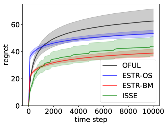
Figure 2: Simulation results for $d=8$ and $r=1$. Our method ESTR-OS, its variant ESTR-BM, and an implicit exploration variant of ESTR called ISSE all outperform the baseline linear bandit method OFUL.

We present a preliminary experimental result and discuss practical concerns.

Bandits in practice requires tuning the exploration rate to perform well, which is usually done by adjusting the confidence bound width Chapelle & Li (2011); Li et al. (2010); Zhang et al. (2016), which amounts to replacing $\beta_{t}$ with $c\beta_{t}$ for some $c>0$ for OFUL or its variants (including LowOFUL). An efficient parameter tuning in bandits is an open problem and is beyond our scope. For the sake of comparison, we tune $c$ by grid search and report the result with the smallest average regret. For ESTR, the value of $T_{1}$ used in the proof involves some unknown constants; to account for this, we tune $T_{1}$ by grid search. We consider the following methods:

• OFUL: The OFUL reduction described in (3), which ignores the low-rank structure.

• ESTR-OS: Our proposed method; we simplify $B_{\perp}$ in (14) to $S_{2}\sigma^{2}d^{3}r/T_{1}$.

• ESTR-BM: We replace OptSpace with the Burer-Monteiro formulation and perform the alternating minimization Burer & Monteiro (2003).

• ISSE (Implicit SubSpace Exploration): LowOFUL with a heuristic subspace estimation that avoids an explicit exploration stage. We split the time intervals with knots at $t\in\{10^{0.5},10^{1},10^{1.5},...\}$. At the beginning time $t^{\prime}$ of each interval, we perform the matrix recovery with the Burer-Monteiro formulation using all the past data, estimate the subspaces, and use them to initialize LowOFUL with $B_{\perp}=S_{2}\sigma^{2}d^{3}r/t^{\prime}$ and all the past data.

Note that OFUL and ISSE only require tuning $c$ whereas ESTR methods require tuning both $c$ and $T_{1}$.

We run our simulation with $d_{1}=d_{2}=8$, $r=1$, $\sigma=0.01$. We set $\lambda=1$ for both OFUL and LowOFUL. We draw 16 arms from the unit sphere for each arm set $\mathcal{X}$ and $\mathcal{Z}$ and simulate the bandit game for $T=10^{4}$ iterations, which we repeat 60 times for each method. Figure 2 plots the average regret of the methods and the .95 confidence intervals. All the methods outperform OFUL, and the regret differences from OFUL are statistically significant. We observe that ESTR-BM performs better than ESTR-OS. We believe this is due to our limit on the number of iterations of OptSpace set to 1000, which we imposed due to its slow convergence in our experiments. The Burer-Monteiro formulation, however, converged within 200 iterations. Finally, ISSE performs close to ESTR-BM, but with a larger variance. Although ISSE does not have a theoretical guarantee, it does not require tuning $T_{1}$ and performs better than OFUL.

7 Related work

There exist a few studies on pulling a pair of arms as a unit action, as we do. Kveton et al. (2017) consider the $K$-armed bandit with $N_{1}$ left arms and $N_{2}$ right arms. The expected rewards can be represented as a matrix $\bar{}\mathbf{R}\in\mathbb{R}^{N_{1}\times N_{2}}$ where the authors assume $\bar{}\mathbf{R}$ has rank $r\ll\min\{N_{1},N_{2}\}$. The main difference from our setting is that they do not assume that the arm features are available, so our work is related to Kveton et al. (2017) in the same way as the linear bandits are related to $K$-armed bandits. The problem considered in Katariya et al. (2017b) is essentially a rank-one version of Kveton et al. (2017), which is motivated by a click-feedback model called position-based model with $N_{1}$ items and $N_{2}$ positions. This work is further extended to have a tighter KL-based bound by Katariya et al. (2017a). All these studies successfully exploit the low-rank structure to enjoy regret bounds that scale with $r(N_{1}+N_{2})$ rather than $N_{1}N_{2}$. Zimmert & Seldin (2018) propose a more generic problem called factored bandits whose action set is a product of atomic $L$ action sets rather than two. While they achieve generality by not require to know the explicit reward model, factored bandits do not leverage the known arm features nor the low-rank structure, resulting in large regret in our problem.

There are other works that exploit the low-rank structure of the reward matrix, although the action is just a single arm pull. Sen et al. (2017) consider the contextual bandit setting where there are $N_{1}$ discrete contexts and $N_{2}$ arms, but do not take into account the observed features of contexts or arms. Under the so-called separability assumption, the authors make use of Hottopix algorithm to exploit the low-rank structure. Gopalan et al. (2016) consider a similar setting, but employ the robust tensor power method for recovery. Kawale et al. (2015) study essentially the same problem, but make assumptions on the prior that generates the unknown matrix and perform online matrix factorization with particle filtering to leverage the low-rank structure. These studies also exploit the low-rank structure successfully and enjoy regret bounds that scale much better than $N_{1}N_{2}$.

There has been a plethora of contextual bandit studies that exploit structures other than the low-rank-ness, where the context is usually the user identity or features. For example, Gentile et al. (2014) and its followup studies Li et al. (2016); Gentile et al. (2017) leverage the clustering structure of the contexts. In Cesa-Bianchi et al. (2013) and Vaswani et al. (2017), a graph structure of the users is leveraged to enjoy regret bound that is lower than running bandits on each context (i.e., user) independently. Deshmukh et al. (2017) introduce a multitask learning view and exploit arm similarity information via kernels, but their regret guarantee is valid only when the similarity is known ahead of time. In this vein, if we think of the right arm set $\mathcal{Z}$ as tasks, we effectively assume different parameters for each task but with a low-rank structure. That is, the parameters can be written as a linear combination of a few hidden factors, which are estimated on the fly rather than being known in advance. Johnson et al. (2016) consider low-rank structured bandits but in a different setup. Their reward model has expected reward of the form ${{\text{tr}}}(\mathbf{X}_{t}^{\top}{{\bm{\Theta}}}^{*})$ with the arm $\mathbf{X}_{t}\in\mathbb{R}^{d\times p}$ and the unknown ${{\bm{\Theta}}}^{*}\in\mathbb{R}^{d\times p}$. While $\mathbf{X}_{t}$ corresponds to $\mathbf{x}_{t}{{\mathbf{z}}}_{t}^{\top}$ in our setting, they consider a continuous arm set only, so their algorithm cannot be applied to our problem.

Our subroutine LowOFUL is quite similar to SpectralUCB of Valko et al. (2014), which is designed specifically for graph-structured arms in which expected rewards of the two arms are close to each other (i.e., “smooth”) when there is an edge between them. Although technical ingredients for Corollary 1 stem from Valko et al. (2014), LowOFUL is for an inherently different setup in which we design the regularization matrix ${{\bm{{\Lambda}}}}$ to maximally exploit the subspace knowledge and minimize the regret, rather than receiving ${{\bm{{\Lambda}}}}$ from the environment as a part of the problem definition. Gilton & Willett (2017) study a similar regularizer in the context of sparse linear bandits under the assumption that a superset of the sparse locations is known ahead of time. Yue et al. (2012b) consider a setup similar to LowOFUL. They assume an estimate of the subspace is available, but their regret bound still depends on the total dimension $p$.

8 Conclusion

In this paper, we introduced the bilinear low-rank bandit problem and proposed the first algorithm with a nontrivial regret guarantee. Our study opens up several future research directions. First, there is currently no nontrivial lower bound, and showing whether the regret of ${\widetilde{\mathcal{O}}}(d^{3/2}\sqrt{rT})$ is tight or not remains open. Second, while our algorithm improves the regret bound over the trivial linear bandit reduction, the algorithm requires to tune an extra parameter $T_{1}$. It would be more natural to continuously update the subspace estimate and the amount of regularization, just like ISSE. However, proving a theoretical guarantee would be challenging since most matrix recovery algorithms require some sort of uniform sampling with a “nice” set of measurements. We speculate that one can employ randomized arm selection and use importance-weighted data to perform effective and provable matrix recoveries on-the-fly.

Appendix A Proof of Theorem 2

Theorem 2 (Restated) There exists a constant $C_{0}$ such that for $T_{1}\geq C_{0}\sigma^{2}(\mu_{0}^{2}+\mu_{1}^{2}){\frac{\kappa^{6}}{\Sigma_{\min}(\mathbf{K}^{*})^{2}}}dr(r+\log d)$, we have that, with probability at least $1-2/d_{2}^{3}$,

$$\|{\widehat{\mathbf{K}}}-\mathbf{K}^{*}\|_{F}\leq C_{1}\kappa^{2}\sigma{\frac{d^{3/2}\sqrt{r}}{\sqrt{T_{1}}}}$$ (15)

where $C_{1}$ is an absolute constant.

Proof.

There are a number of assumptions required for the guarantee of OptSpace to hold. Given a noise matrix $\mathbf{Z}$, let $\widetilde{\mathbf{K}}=\mathbf{K}^{*}+\mathbf{Z}$ be the noisy observation of matrix $\mathbf{K}^{*}$. Among various noise models in Keshavan et al. (2010, Theorem 1.3), the independent $\rho$-sub-Gaussian model fits our problem setting well. Let $E\in[m]\times[n]$ be the indicator of observed entries and let $\mathbf{Z}^{E}$ be a censored version of $\mathbf{Z}$ in which the unobserved entries are zeroed out. Recall that we assume $d_{2}=\Theta(d_{1})$, that $d=\max\{d_{1},d_{2}\}$, and that $\kappa$ is the condition number of $\mathbf{K}^{*}$.

We first state the guarantee and then describe the required technical assumptions. Keshavan et al. (2010, Theorem 1.2) states that the following is true for some constant $C^{\prime}>0$:

$$\|{\widehat{\mathbf{K}}}-\mathbf{K}^{*}\|_{F}\leq C^{\prime}\kappa^{2}{\frac{d^{2}\sqrt{r}}{|E|}}\|\mathbf{Z}^{E}\|_{2}\;.$$

Here, by Keshavan et al. (2010, Theorem 1.3), $\|\mathbf{Z}^{E}\|_{2}$ is no larger than $C^{\prime\prime}\rho\sqrt{|E|/d}$, for some constant $C^{\prime\prime}>0$, under Assumption (A3) below, where $\rho$ is the sub-Gaussian scale parameter for the noise $\mathbf{Z}$. ($\rho$ can be different from $\sigma$, as we explain below). The original version of the statement has a preprocessed version $\|\tilde{}\mathbf{Z}^{E}\|_{2}$ rather than $\|\mathbf{Z}^{E}\|_{2}$, but they are the same under our noise model, according to Keshavan et al. (2010, Section 1.5). Together, in our notation, we have

$$\|{\widehat{\mathbf{K}}}-\mathbf{K}^{*}\|_{F}\leq C^{\prime}C^{\prime\prime}\kappa^{2}\rho{\frac{d^{3/2}\sqrt{r}}{\sqrt{|E|}}}.$$

In the case of $T_{1}<d_{1}d_{2}$, the guarantee above holds true with $\rho=\sigma$ and $|E|=T_{1}$. If $T_{1}\geq d_{1}d_{2}$, the guarantee holds true with $\rho=\sigma\cdot\left(\left\lfloor{\frac{T_{1}}{d_{1}d_{2}}}\right\rfloor\right)^{-1/2}$ and $|E|=d_{1}d_{2}$. In both cases, we arrive at (6).

We now state the conditions. Let $\alpha=d_{1}/d_{2}$. Define ${\Sigma_{\min}}$ to be the smallest nonzero singular values of $\mathbf{M}$.

• (A1): $\mathbf{M}$ is $({\mu_{0}},{\mu_{1}})$-incoherent. Note $\mu_{0}\in[1,\max\{d_{1},d_{2}\}/r]$.

• (A2): (Sufficient observation) For some $C^{\prime}>0$, we have

  $$|E|\geq C^{\prime}d_{2}\sqrt{\alpha}\kappa^{2}\max\left\{\mu_{0}r\sqrt{\alpha}\log d_{2},\;\mu_{0}^{2}r^{2}\alpha\kappa^{4},\;\mu_{1}^{2}r^{2}\alpha\kappa^{4}\right\}\;,$$

  which we loosen and simplify to (using $\mu_{0}\geq 1$)

  $$|E|\geq C^{\prime}\kappa^{6}(\mu_{0}^{2}+\mu_{1}^{2})dr(r+\log d).$$

• (A3): $|E|\geq n\log n$.

• (A4): We combine the bound on $\|\mathbf{Z}^{E}\|_{2}$ and the condition in Keshavan et al. (2010, Theorem 1.2) that says “provided that the RHS is smaller than $\sigma_{\min}$”, which results in requiring

  $${\frac{|E|}{\rho^{2}}}\geq C^{\prime\prime}{\frac{\kappa^{4}}{\Sigma_{\min}^{2}}}dr,$$

  for some $C^{\prime\prime}>0$, Using the same logic as before, either $T_{1}<d_{1}d_{2}$ or $T_{1}\geq d_{1}d_{2}$, we can rewrite the same statement in terms of $T_{1}$, as follows:

  $$T_{1}\geq C^{\prime\prime}\sigma^{2}{\frac{\kappa^{4}}{\Sigma_{\min}^{2}}}dr\;.$$

All these conditions can be merged to

$$T_{1}\geq C_{0}\sigma^{2}(\mu_{0}^{2}+\mu_{1}^{2}){\frac{\kappa^{6}}{\Sigma_{\min}^{2}}}dr(r+\log d)$$

for some constant $C_{0}>0$. ∎

Appendix B Proof of Theorem 3

We first restate the $\sin\Theta$ theorem due to Wedin Stewart & Sun (1990) in a slightly simplified form. Let the SVDs of matrices $\mathbf{A}$ and $\tilde{}\mathbf{A}$ be defined as follows:

$$(\mathbf{U}_{1}\;\mathbf{U}_{2}\;\mathbf{U}_{3})^{\top}\mathbf{A}(\mathbf{V}_{1}\;\mathbf{V}_{2})=\begin{pmatrix}\mathbf{\Sigma}_{1}&\mathbf{0}\\ \mathbf{0}&\mathbf{\Sigma}_{2}\\ \mathbf{0}&\mathbf{0}\end{pmatrix},$$

$$(\tilde{}\mathbf{U}_{1}\;\tilde{}\mathbf{U}_{2}\;\tilde{}\mathbf{U}_{3})^{\top}\tilde{}\mathbf{A}(\tilde{}\mathbf{V}_{1}\;\tilde{}\mathbf{V}_{2})=\begin{pmatrix}\tilde{}\mathbf{\Sigma}_{1}&\mathbf{0}\\ \mathbf{0}&\tilde{}\mathbf{\Sigma}_{2}\\ \mathbf{0}&\mathbf{0}\end{pmatrix}.$$

Let $\mathbf{R}=\mathbf{A}\tilde{}\mathbf{V}_{1}-\tilde{}\mathbf{U}_{1}\tilde{}\mathbf{\Sigma}_{1}$ and $\mathbf{S}=\mathbf{A}^{\top}\tilde{}\mathbf{U}_{1}-\tilde{}\mathbf{V}_{1}\tilde{}\mathbf{\Sigma}_{1}$, and define $\mathbf{U}_{1\perp}=[\mathbf{U}_{2}\;\mathbf{U}_{3}]$ and $\mathbf{V}_{1\perp}=[\mathbf{V}_{2}\;\mathbf{V}_{3}]$. Wedin’s $\sin\Theta$ theorem, roughly speaking, bounds the sin canonical angles between two matrices by the Frobenius norm of their difference.

Theorem 6 (Wedin).

Suppose that there is a number $\delta>0$ such that

$$\min_{i,j}\left|\sigma_{i}\left(\tilde{}\mathbf{\Sigma}_{1}\right)-\sigma_{j}\left(\mathbf{\Sigma}_{2}\right)\right|\geq\delta\quad\text{ and }\quad\min_{i}\sigma_{i}\left(\tilde{}\mathbf{\Sigma}_{1}\right)\geq\delta\;.$$

Then,

$$\sqrt{\|\mathbf{U}_{1\perp}^{\top}\tilde{}\mathbf{U}_{1}\|_{F}^{2}+\|\mathbf{V}_{1\perp}^{\top}\tilde{}\mathbf{V}_{1}\|_{F}^{2}}\leq{\frac{\sqrt{\|\mathbf{R}\|_{F}^{2}+\|\mathbf{S}\|_{F}^{2}}}{\delta}}$$

We now prove Theorem 3.

Theorem 3 (Restated) Suppose we invoke OptSpace to compute ${\widehat{\mathbf{K}}}$ as an estimate of the matrix $\mathbf{K}^{*}$. After stage 1 of ESTR with $T_{1}$ satisfying the condition of Theorem 2, we have, with probability at least $1-2/d_{2}^{3}$,

$$\|{\widehat{\mathbf{U}}}_{\perp}^{\top}\mathbf{U}^{*}\|_{F}\|{\widehat{\mathbf{V}}}_{\perp}^{\top}\mathbf{V}^{*}\|_{F}\leq{\frac{\|\mathbf{X}^{-1}\|_{2}^{2}\|\mathbf{Z}^{-1}\|_{2}^{2}}{(s^{*}_{r})^{2}}}\tau^{2}$$ (16)

where $\tau=C_{1}\kappa^{2}\sigma{d^{3/2}\sqrt{r}}/{\sqrt{T_{1}}}$.

Proof.

In our case, the variables defined for Wedin’s theorem are as follows:

$$\mathbf{A} ={\widehat{{{\bm{\Theta}}}}} \tilde{}\mathbf{A} ={{\bm{\Theta}}}^{*}$$

$$\mathbf{U}_{1} ={\widehat{\mathbf{U}}} \tilde{}\mathbf{U}_{1} =\mathbf{U}^{*}$$

$$\mathbf{\Sigma}_{1} ={\widehat{\mathbf{S}}} \tilde{}\mathbf{\Sigma}_{1} =\mathbf{S}^{*}$$

$$\mathbf{V}_{1} ={\widehat{\mathbf{V}}} \tilde{}\mathbf{V}_{1} =\mathbf{V}^{*}\;.$$

Let ${\mathbf{E}}={\widehat{{{\bm{\Theta}}}}}-{{\bm{\Theta}}}^{*}$. Note that

$$\mathbf{R} ={\widehat{{{\bm{\Theta}}}}}\mathbf{V}^{*}-\mathbf{U}^{*}\mathbf{S}^{*}=({{\bm{\Theta}}}^{*}+\mathbf{E})\mathbf{V}^{*}-\mathbf{U}^{*}\mathbf{S}^{*}=\mathbf{E}{\widehat{\mathbf{V}}}$$

$$\mathbf{S} =-\mathbf{E}^{\top}\mathbf{U}^{*}\quad(\text{similarly})\;.$$

Then, $\|\mathbf{R}\|_{F}=\|\mathbf{E}{\widehat{\mathbf{V}}}\|_{F}\leq\|\mathbf{E}\|_{F}$, using the fact that

$$\|\mathbf{E}\|_{F}=\|\mathbf{E}[{\widehat{\mathbf{V}}}\;{\widehat{\mathbf{V}}}_{\perp}]\|_{F}=\sqrt{\|\mathbf{E}{\widehat{\mathbf{V}}}\|_{F}^{2}+\|\mathbf{E}{\widehat{\mathbf{V}}}_{\perp}\|_{F}^{2}}.$$

Similarly, $\|\mathbf{S}\|_{F}\leq\|\mathbf{E}\|_{F}$. We now apply the $\sin\Theta$ theorem to obtain

$$\sqrt{2\|{\widehat{\mathbf{U}}}_{\perp}^{\top}\mathbf{U}^{*}\|_{F}\|{\widehat{\mathbf{V}}}_{\perp}^{\top}\mathbf{V}^{*}\|_{F}}\leq\sqrt{\|{\widehat{\mathbf{U}}}_{\perp}^{\top}\mathbf{U}^{*}\|_{F}^{2}+\|{\widehat{\mathbf{V}}}_{\perp}^{\top}\mathbf{V}^{*}\|_{F}^{2}}\leq{\frac{\sqrt{\|\mathbf{R}\|_{F}^{2}+\|\mathbf{S}\|_{F}^{2}}}{{\delta}}}\leq{\frac{\sqrt{2\|\mathbf{E}\|_{F}^{2}}}{s^{*}_{r}}}$$

where the first inequality follows from the Young’s inequality. To summarize, we have

$$\|{\widehat{\mathbf{U}}}_{\perp}^{\top}\mathbf{U}^{*}\|_{F}\|{\widehat{\mathbf{V}}}_{\perp}^{\top}\mathbf{V}^{*}\|_{F}\leq{\frac{\|{{\bm{\Theta}}}^{*}-{\widehat{{{\bm{\Theta}}}}}\|_{F}^{2}}{s_{r}^{*2}}}\;.$$ (17)

Theorem 2 and the inequality $\|{\widehat{{{\bm{\Theta}}}}}-{{\bm{\Theta}}}^{*}\|_{F}\leq\|\mathbf{X}^{-1}\|_{2}\|\mathbf{Z}^{-1}\|_{2}\|{\widehat{\mathbf{K}}}-\mathbf{K}^{*}\|_{F}$ conclude the proof. ∎

Appendix C Proof of Lemma 1

This lemma is a direct consequence of Valko et al. (2014, Lemma 3). We just need to characterize the constant $C$ therein that upper bounds $\|{\bm{\theta}}^{*}\|_{{\bm{{\Lambda}}}}$. The observation that

$$\|{\bm{\theta}}^{*}\|_{{\bm{{\Lambda}}}}\leq\sqrt{\lambda\|{\bm{\theta}}_{1:k}\|_{2}^{2}+\lambda_{\perp}\|{\bm{\theta}}_{k+1:p}\|_{2}^{2}}\leq\sqrt{\lambda}S+\sqrt{\lambda_{\perp}}S_{\perp}$$

completes the proof.

Appendix D Proof of Theorem 4

Let $r_{t}$ be the instantaneous pseudo-regret at time $t$: $r_{t}={\langle}{\bm{\theta}}^{*},\mathbf{a}^{*}{\rangle}-{\langle}{\bm{\theta}}^{*},\mathbf{a}_{t}{\rangle}$. The assumptions $\|\mathbf{a}_{t}\|_{2}\leq 1$ and $||{\bm{\theta}}^{*}||_{2}\leq B$ imply that $r_{t}\leq 2B$. Using the fact that the OFUL ellipsoidal confidence set contains ${\bm{\theta}}^{*}$ w.p. $\geq 1-{\delta}$, one can show that $r_{t}\leq 2\sqrt{\beta_{t}}\|\mathbf{x}_{t}\|_{\mathbf{V}_{t-1}^{-1}}$ as shown in Abbasi-Yadkori et al. (2011, Theorem 3). Then, using the monotonicity of $\beta_{t}$,

$$r_{t} \leq\min\{2B,2\sqrt{\beta_{{t}}}\|\mathbf{x}_{t}\|_{\mathbf{V}_{t-1}^{-1}}\}\leq\min\{2B,2\sqrt{\beta_{{T}}}\|\mathbf{x}_{t}\|_{\mathbf{V}_{t-1}^{-1}}\}$$

$$=2\sqrt{\beta_{T}}\min\{B/\sqrt{\beta_{T}},\|\mathbf{x}_{t}\|_{\mathbf{V}_{t-1}^{-1}}\}$$

$$\implies\sum_{t=1}^{T}r_{t} \stackrel{{\scriptstyle(a)}}{{\leq}}2\sqrt{\beta_{T}}\sqrt{T\sum_{t=1}^{T}\min\{B^{2}/\beta_{T},\|\mathbf{x}_{t}\|^{2}_{\mathbf{V}_{t-1}^{-1}}\}}$$

$$\stackrel{{\scriptstyle(b)}}{{\leq}}2\sqrt{\beta_{T}}\sqrt{T\max\{2,B^{2}/\beta_{T}\}\sum_{t=1}^{T}\log\left(1+\|\mathbf{x}_{t}\|^{2}_{\mathbf{V}_{t-1}^{-1}}\right)}$$

$$\stackrel{{\scriptstyle(c)}}{{\leq}}2\sqrt{\max\{2,1/{\lambda}\}}\sqrt{\beta_{T}}\sqrt{\log{\frac{|\mathbf{V}_{T}|}{|{{\bm{{\Lambda}}}}|}}}\sqrt{T}$$

where $(a)$ is due to Cauchy-Schwarz, $(b)$ is due to $\min\{a,x\}\leq\max\{2,a\}\log(1+x),\forall a,x>0$ (see Jun et al. (2017, Lemma 3)), and $(c)$ is by $\sum_{t=1}^{T}\log(1+\|\mathbf{x}_{t}\|^{2}_{\mathbf{V}_{t-1}^{-1}})=\log{\frac{|\mathbf{V}_{T}|}{|{{\bm{{\Lambda}}}}|}}$ (see Abbasi-Yadkori et al. (2011, Lemma 11)) and $\beta_{T}\geq(\sqrt{{\lambda}}B+\sqrt{\lambda_{\perp}}B_{\perp})^{2}\geq{\lambda}B^{2}$.

Appendix E Proof of Corollary 1

The lemma from Valko et al. (2014) characterizes how large $\log{\frac{|\mathbf{V}_{T}|}{|{{\bm{{\Lambda}}}}|}}$ can be.

Lemma 2.

(Valko et al., 2014, Lemma 5) For any $T$, let ${{\bm{{\Lambda}}}}=\mbox{diag}([{\lambda}_{1},\ldots,{\lambda}_{p}])$.

$$\log{\frac{|\mathbf{V}_{T}|}{|{{\bm{{\Lambda}}}}|}}\leq\max\sum_{i=1}^{p}\log\left(1+{\frac{t_{i}}{{\lambda}_{i}}}\right)$$

where the maximum is taken over all possible positive real numbers $t_{1},\ldots,t_{p}$ such that $\sum_{i=1}^{p}t_{i}=T$.

We specify a desirable value of $\lambda_{\perp}$ in the following lemma.

Lemma 3.

If $\lambda_{\perp}={\frac{T}{k\log\left(1+{\frac{T}{{\lambda}}}\right)}}$, then

$$\log{\frac{|\mathbf{V}_{T}|}{|{{\bm{{\Lambda}}}}|}}\leq 2k\log\left(1+{\frac{T}{{\lambda}}}\right)$$

Proof.

Inheriting the setup of Lemma 2,

$$\log{\frac{|\mathbf{V}_{T}|}{|{{\bm{{\Lambda}}}}|}} \leq\max\sum_{i=1}^{p}\log(1+{\frac{t_{i}}{{\lambda}_{i}}})$$

$$\leq k\log(1+{\frac{T}{{\lambda}}})+\sum_{i=k+1}^{p}\log(1+{\frac{t_{i}}{\lambda_{\perp}}})$$

Then,

$$\sum_{i=k+1}^{p}\log(1+{\frac{t_{i}}{\lambda_{\perp}}})\leq\sum_{i=k+1}^{p}{\frac{t_{i}}{\lambda_{\perp}}}\leq{\frac{T}{\lambda_{\perp}}}=k\log(1+T/{\lambda})\;.$$

∎

By Lemma 3, the regret bound is, ignoring constants,

$$\left(\sigma k\log(1+T/{\lambda})+\sqrt{k\log(1+T/{\lambda})}\cdot(\sqrt{{\lambda}}S+\sqrt{\lambda_{\perp}}S_{\perp})\right)\cdot\sqrt{T} ={\widetilde{\mathcal{O}}}\left(\left(\sigma k+\sqrt{k}\cdot(\sqrt{\lambda}S+\sqrt{\lambda_{\perp}}S_{\perp})\right)\sqrt{T}\right)$$

$$={\widetilde{\mathcal{O}}}((\sigma k+\sqrt{k\lambda}S+\sqrt{k}\cdot\sqrt{{\frac{T}{k}}}S_{\perp})\sqrt{T})$$

$$={\widetilde{\mathcal{O}}}((\sigma k+\sqrt{k\lambda}S+\sqrt{T}S_{\perp})\sqrt{T})$$

Appendix F Proof of Theorem 5 and Corollary 2

Let us define $r_{t}=\max_{\mathbf{x}\in\mathcal{X},{{\mathbf{z}}}\in\mathcal{Z}}\mathbf{x}^{\top}{{\bm{\Theta}}}^{*}{{\mathbf{z}}}-\mathbf{x}_{t}^{\top}{{\bm{\Theta}}}^{*}{{\mathbf{z}}}_{t}$, the instantaneous regret at time $t$. Using $\max_{\|x\|_{2},\|z\|_{2}\leq 1}$ $|\mathbf{x}^{\top}{{\bm{\Theta}}}^{*}{{\mathbf{z}}}|\leq\|{{\bm{\Theta}}}^{*}\|_{2}$, we bound the cumulative regret incurred up to the stage 1 as $\sum_{t=1}^{T_{1}}r_{t}\leq 2S_{2}T_{1}$. In the second stage, by the choices of $S$ and $S_{F}$ of (14),

$$\sum_{t=T_{1}+1}^{T_{2}}r_{t} ={\widetilde{\mathcal{O}}}((\sigma k+\sqrt{k{\lambda}}S+\sqrt{T_{2}}S_{\perp})\sqrt{T_{2}})$$

$$={\widetilde{\mathcal{O}}}\left(\left(\sigma k+\sqrt{k{\lambda}}S_{F}+\sqrt{T_{2}}\cdot\|\mathbf{X}^{-1}\|_{2}^{2}\|\mathbf{Z}^{-1}\|_{2}^{2}C_{1}^{2}{\frac{S_{2}^{5}}{S_{r}^{6}}}\sigma^{2}d^{3}r\cdot{\frac{1}{T_{1}}}\right)\sqrt{T_{2}}\right)$$

Then, the overall regret is, using $T_{2}\leq T$

$$\sum_{t=1}^{T}r_{t}={\widetilde{\mathcal{O}}}\left(s^{*}_{1}T_{1}+T\cdot\|\mathbf{X}^{-1}\|_{2}^{2}\|\mathbf{Z}^{-1}\|_{2}^{2}{\frac{S_{2}^{5}}{S_{r}^{6}}}\sigma^{2}d^{3}r\cdot{\frac{1}{T_{1}}}\right)$$

With the choice of $T_{1}=\Theta\left(\sqrt{T\|\mathbf{X}^{-1}\|_{2}^{2}\|\mathbf{Z}^{-1}\|_{2}^{2}{\frac{S_{2}^{4}}{S_{r}^{6}}}\sigma^{2}d^{3}r}\right)$, the regret is

$${\widetilde{\mathcal{O}}}\left({\frac{S_{2}^{3}}{S_{r}^{3}}}\|\mathbf{X}^{-1}\|_{2}\|\mathbf{Z}^{-1}\|_{2}\sigma d^{3/2}\sqrt{rT}\right)$$

Appendix G Heuristics for selecting arms in stage 1

We describe heuristics for solving (4) when the arm set is finite.

Let $\mathbf{X}\in\mathbb{R}^{N_{1}\times d_{1}}$ be a matrix that takes each arm $\mathbf{x}\in\mathcal{X}$ as its row. One way to develop algorithms for solving (4) is to relax the cardinality constraint to a continuous one:

$$\begin{array}[]{rrclcl}\displaystyle\min_{{{\bm{{\lambda}}}}}&\lx@intercol-t\hfil\lx@intercol\\ \mbox{s.t.}&\mathbf{X}^{\top}\mbox{diag}({{\bm{{\lambda}}}})\mathbf{X}&\succeq&t\mathbf{I}\\ &{\lambda}_{i}&\geq&0\quad\forall i\in[N_{1}]\\ &\sum_{i=1}^{N_{1}}{\lambda}_{i}&=&1\\ \end{array}$$

We then choose the top $d_{1}$ arms with the largest ${\lambda}_{i}$.

We found that choosing the best among the solution above and 20 candidate subsets drawn uniformly at random (total 21 candidate subsets) returns reasonable solutions for our purpose.

References

- Abbasi-Yadkori et al. (2009) Abbasi-Yadkori, Y., Antos, A., and Szepesvári, C. Forced-exploration based algorithms for playing in stochastic linear bandits. In COLT Workshop on On-line Learning with Limited Feedback. Citeseer, 2009.
- Abbasi-Yadkori et al. (2011) Abbasi-Yadkori, Y., Pal, D., and Szepesvari, C. Improved Algorithms for Linear Stochastic Bandits. Advances in Neural Information Processing Systems (NeurIPS), pp. 1–19, 2011.
- Auer (2002) Auer, P. Using Confidence Bounds for Exploitation-Exploration Trade-offs. Journal of Machine Learning Research, 3:2002, 2002.
- Auer et al. (2002) Auer, P., Cesa-Bianchi, N., and Fischer, P. Finite-time Analysis of the Multiarmed Bandit Problem. Machine Learning, 47(2–3):235–256, 2002.
- Bhargava et al. (2017) Bhargava, A., Ganti, R., and Nowak, R. Active Positive Semidefinite Matrix Completion: Algorithms, Theory and Applications. In Proceedings of the International Conference on Artificial Intelligence and Statistics (AISTATS), volume 54, pp. 1349–1357, 2017.
- Bubeck & Cesa-Bianchi (2012) Bubeck, S. and Cesa-Bianchi, N. Regret Analysis of Stochastic and Nonstochastic Multi-armed Bandit Problems. Foundations and Trends in Machine Learning, 5:1–122, 2012.
- Burer & Monteiro (2003) Burer, S. and Monteiro, R. D. C. A nonlinear programming algorithm for solving semidefinite programs via low-rank factorization. Mathematical Programming, Series B, 2003.
- Cai et al. (2015) Cai, T. T., Zhang, A., and Others. ROP: Matrix recovery via rank-one projections. The Annals of Statistics, 43(1):102–138, 2015.
- Çivril & Magdon-Ismail (2007) Çivril, A. and Magdon-Ismail, M. Finding maximum Volume sub-matrices of a matrix. RPI Comp Sci Dept TR, pp. 7–8, 2007.
- Çivril & Magdon-Ismail (2009) Çivril, A. and Magdon-Ismail, M. On selecting a maximum volume sub-matrix of a matrix and related problems. Theoretical Computer Science, 410(47):4801, 2009.
- Cesa-Bianchi et al. (2013) Cesa-Bianchi, N., Gentile, C., and Zappella, G. A Gang of Bandits. In Burges, C. J. C., Bottou, L., Welling, M., Ghahramani, Z., and Weinberger, K. Q. (eds.), Advances in Neural Information Processing Systems (NeurIPS), pp. 737–745. 2013.
- Chapelle & Li (2011) Chapelle, O. and Li, L. An Empirical Evaluation of Thompson Sampling. In Advances in Neural Information Processing Systems (NeurIPS), pp. 2249–2257, 2011.
- Dani et al. (2008) Dani, V., Hayes, T. P., and Kakade, S. M. Stochastic Linear Optimization under Bandit Feedback. In Proceedings of the Conference on Learning Theory (COLT), pp. 355–366, 2008.
- Deshmukh et al. (2017) Deshmukh, A. A., Dogan, U., and Scott, C. Multi-Task Learning for Contextual Bandits. In Advances in Neural Information Processing Systems (NeurIPS), pp. 4848–4856. 2017.
- Filippi et al. (2010) Filippi, S., Cappe, O., Garivier, A., and Szepesvári, C. Parametric Bandits: The Generalized Linear Case. In Advances in Neural Information Processing Systems (NeurIPS), pp. 586–594. 2010.
- Gentile et al. (2014) Gentile, C., Li, S., and Zappella, G. Online Clustering of Bandits. In Proceedings of the International Conference on Machine Learning (ICML), volume 32, pp. 757–765, 2014.
- Gentile et al. (2017) Gentile, C., Li, S., Kar, P., Karatzoglou, A., Zappella, G., and Etrue, E. On Context-Dependent Clustering of Bandits. In Proceedings of the International Conference on Machine Learning (ICML), volume 70, pp. 1253–1262, 2017.
- Gilton & Willett (2017) Gilton, D. and Willett, R. Sparse linear contextual bandits via relevance vector machines. In International Conference on Sampling Theory and Applications (SampTA), pp. 518–522, 2017.
- Gopalan et al. (2016) Gopalan, A., Maillard, O.-A., and Zaki, M. Low-rank Bandits with Latent Mixtures. arXiv:1609.01508 [cs.LG], 2016.
- Johnson et al. (2016) Johnson, N., Sivakumar, V., and Banerjee, A. Structured Stochastic Linear Bandits. arXiv:1606.05693 [stat.ML], 2016.
- Jun et al. (2017) Jun, K.-S., Bhargava, A., Nowak, R., and Willett, R. Scalable Generalized Linear Bandits: Online Computation and Hashing. In Advances in Neural Information Processing Systems (NeurIPS), pp. 99–109. 2017.
- Katariya et al. (2017a) Katariya, S., Kveton, B., Szepesvári, C., Vernade, C., and Wen, Z. Bernoulli Rank-1 Bandits for Click Feedback. In Proceedings of the International Joint Conference on Artificial Intelligence (IJCAI), pp. 2001–2007, 2017a.
- Katariya et al. (2017b) Katariya, S., Kveton, B., Szepesvári, C., Vernade, C., and Wen, Z. Stochastic Rank-1 Bandits. In Proceedings of the International Conference on Artificial Intelligence and Statistics (AISTATS), pp. 392–401, 2017b.
- Kawale et al. (2015) Kawale, J., Bui, H. H., Kveton, B., Tran-Thanh, L., and Chawla, S. Efficient Thompson Sampling for Online Matrix-Factorization Recommendation. In Advances in Neural Information Processing Systems (NeurIPS), pp. 1297–1305. 2015.
- Keshavan et al. (2010) Keshavan, R. H., Montanari, A., and Oh, S. Matrix Completion from Noisy Entries. J. Mach. Learn. Res., 11:2057–2078, 2010. ISSN 1532-4435.
- Kveton et al. (2017) Kveton, B., Szepesvári, C., Rao, A., Wen, Z., Abbasi-Yadkori, Y., and Muthukrishnan, S. Stochastic Low-Rank Bandits. arXiv:1712.04644 [cs.LG], 2017.
- Lai & Robbins (1985) Lai, T. L. and Robbins, H. Asymptotically Efficient Adaptive Allocation Rules. Advances in Applied Mathematics, 6(1):4–22, 1985.
- Lattimore & Szepesvári (2018) Lattimore, T. and Szepesvári, C. Bandit Algorithms. 2018. URL http://downloads.tor-lattimore.com/book.pdf.
- Li et al. (2010) Li, L., Chu, W., Langford, J., and Schapire, R. E. A Contextual-Bandit Approach to Personalized News Article Recommendation. Proceedings of the International Conference on World Wide Web (WWW), pp. 661–670, 2010.
- Li et al. (2016) Li, S., Karatzoglou, A., and Gentile, C. Collaborative Filtering Bandits. In Proceedings of the International ACM SIGIR Conference on Research and Development in Information Retrieval (SIGIR), pp. 539–548, 2016.
- Luo et al. (2017) Luo, Y., Zhao, X., Zhou, J., Yang, J., Zhang, Y., Kuang, W., Peng, J., Chen, L., and Zeng, J. A network integration approach for drug-target interaction prediction and computational drug repositioning from heterogeneous information. Nature communications, 8(1):573, 2017.
- Ma et al. (2008) Ma, H., Yang, H., Lyu, M. R., and King, I. SoRec: Social Recommendation Using Probabilistic Matrix Factorization. Proceeding of the ACM Conference on Information and Knowledge Mining (CIKM), 2008.
- Mohan & Fazel (2010) Mohan, K. and Fazel, M. New restricted isometry results for noisy low-rank recovery. In IEEE International Symposium on Information Theory - Proceedings, 2010.
- Recht et al. (2010) Recht, B., Fazel, M., and Parrilo, P. A. Guaranteed Minimum-Rank Solutions of Linear Matrix Equations via Nuclear Norm Minimization. SIAM Rev., 52(3):471–501, 2010.
- Rusmevichientong & Tsitsiklis (2010) Rusmevichientong, P. and Tsitsiklis, J. N. Linearly Parameterized Bandits. Math. Oper. Res., 35(2):395–411, 2010.
- Sen et al. (2017) Sen, R., Shanmugam, K., Kocaoglu, M., Dimakis, A., and Shakkottai, S. Contextual Bandits with Latent Confounders: An NMF Approach. In Proceedings of the International Conference on Artificial Intelligence and Statistics (AISTATS), volume 54, pp. 518–527, 2017.
- Stewart & Sun (1990) Stewart, G. W. and Sun, J.-g. Matrix Perturbation Theory. Academic Press, 1990.
- Tropp (2009) Tropp, J. A. Column subset selection, matrix factorization, and eigenvalue optimization. In Proceedings of the Twentieth Annual ACM-SIAM Symposium on Discrete Algorithms, pp. 978–986. Society for Industrial and Applied Mathematics, 2009.
- Valko et al. (2014) Valko, M., Munos, R., Kveton, B., and Kocak, T. Spectral Bandits for Smooth Graph Functions. In Proceedings of the International Conference on Machine Learning (ICML), pp. 46–54, 2014.
- Vaswani et al. (2017) Vaswani, S., Schmidt, M., and Lakshmanan, L. V. S. Horde of Bandits using Gaussian Markov Random Fields. In Proceedings of the International Conference on Artificial Intelligence and Statistics (AISTATS), pp. 690–699, 2017.
- Yue et al. (2012a) Yue, Y., Broder, J., Kleinberg, R., and Joachims, T. The K-armed dueling bandits problem. In Journal of Computer and System Sciences, 2012a.
- Yue et al. (2012b) Yue, Y., Hong, S. A. S., and Guestrin, C. Hierarchical exploration for accelerating contextual bandits. Proceedings of the International Conference on Machine Learning (ICML), pp. 1895–1902, 2012b.
- Zhang et al. (2016) Zhang, L., Yang, T., Jin, R., Xiao, Y., and Zhou, Z.-h. Online Stochastic Linear Optimization under One-bit Feedback. In Proceedings of the International Conference on Machine Learning (ICML), volume 48, pp. 392–401, 2016.
- Zimmert & Seldin (2018) Zimmert, J. and Seldin, Y. Factored Bandits. In Advances in Neural Information Processing Systems (NeurIPS), pp. 2840–2849, 2018.
Supplementary Material