A focusing and defocusing semi-discrete complex short pulse equation and its varioius soliton solutions

Abstract

In this paper, we are concerned with a a semi-discrete complex short pulse (CSP) equation of both focusing and defocusing types, which can be viewed as an analogue to the Ablowitz-Ladik (AL) lattice in the ultra-short pulse regime. By using a generalized Darboux transformation method, various solutions to this newly integrable semi-discrete equation are studied with both zero and nonzero boundary conditions. To be specific, for the focusing CSP equation, the multi-bright solution (zero boundary condition), multi-breather and high-order rogue wave solutions (nonzero boudanry conditions) are derived, while for the defocusing CSP equation with nonzero boundary condition, the multi-dark soliton solution is constructed. We further show that, in the continuous limit, all the solutions obtained converge to the ones for its original CSP equation (see Physica D, 327 13-29 and Phys. Rev. E 93 052227)
Key words: generalized Darboux transformation, semi-discrete complex short pulse equation, bright and dark soliton, breather, rogue wave
Mathematics Subject Classification: 39A10, 35Q58

I Introduction

The most recent advances in nonlinear optics include the generation and applications of ultrashort optical pulses, whose time duration is typically of the order of femtoseconds, which lead to the Nobel prize in physics 2018 2018Nobelprize . It has been an important topics for the mathematical models of optical pulse propagation in medium Agrawalbook ; HasegawaKodama ; AgrawalKivsharbook . When the range of short pulse width is from 10 $ns$ to 10 $fs$, both dispersive and nonlinear effects influence their shape and spectrum. The following full wave equation

$$\nabla^{2}\mathbf{E}-\frac{1}{c^{2}}\mathbf{E}_{tt}=\mu_{0}\mathbf{P}_{tt}\,,$$ (1)

originates directly from Maxwell’s equation. If we assume the local medium response and only the third-order nonlinear effects (Kerr effect) the induced polarization consists of linear and nonlinear parts, $\mathbf{P}(\mathbf{r},t)=\mathbf{P}_{L}(\mathbf{r},t)+\mathbf{P}_{NL}(\mathbf{r},t)$.

Under the assumption of quasi-monochromatic, i.e., the pulse spectrum, centered as $\omega_{0}$, is assumed to have a spectral width $\Delta\omega$ such that $\Delta\omega/\omega_{0}<<1$. Under this assumption, one can expand the frequency-dependent dielectric constant $\epsilon(\omega)$ in terms of Taylor series up to the second order. As a result, the so-called nonlinear Schrödinger equation

$$\mathrm{i}q_{z}+\alpha_{1}q_{\tau\tau}+\alpha_{2}|q|^{2}q=0\,,$$ (2)

can be derived to govern the slowly varying envelop of optical waves in weakly nonlinear dispersive media HasegawaTappert1 ; HasegawaTappert2 . Here $\alpha_{1}$ represents the effect of group velocity dispersion (GVD) ($\alpha_{1}>0$ corresponds to anomalous dispersion, also focusing case, and $\alpha_{1}<0$–normal dispersion, also defocusing case), $\alpha_{2}$ represents the self-phase modulation (SPM) due to Kerr effect.

Upon switching the spatial and temporal variables and normalization, the nonlinear Schrödinger (NLS) equation can be put into a standard form

$${\mathrm{i}}q_{t}=q_{xx}+2\sigma|q|^{2}q\,$$ (3)

which has become a generic model equation describing the evolution of small amplitude and slowly varying wave packets in weakly nonlinear media Agrawalbook ; HasegawaKodama ; AgrawalKivsharbook ; Ablowitzbook ; APT . It arises in a variety of physical contexts such as nonlinear optics metioned above, Bose-Einstein condesates BECReview , water waves Benney1967 and plasma physics ZakharovPlasma . The integrability, as well as the bright-soliton solution in the focusing case ($\sigma=1$), was found by Zakharov and Shabat ZakharovShabat ; ZakharovShabat2 . The dark soliton was found in the defocusing NLS equation ($\sigma=-1$) HasegawaTappert2 , and was observed experimentally in 1988 Krokeldark1 ; Weinerdark1 . Recently, the rogue (freak) waves were discovered and the Peregrine soliton was found in focusing NLS equation Opticalroguewave ; Peregrinesoliton .

The integrable discretization of nonlinear Schrödinger equation

$$\mathrm{i}q_{n,t}=\left(1+\sigma|q_{n}|^{2}\right)\left(q_{n+1}+q_{n-1}\right)\,$$ (4)

was originally derived by Ablowitz and Ladik AblowitzLadik ; AL2 , so it is also called the Ablowitz-Ladik (AL) lattice equation. Similar to the continuous case, it is known that the AL lattice equation, by Hirota’s bilinear method, admits the bright soliton solution for the focusing case ($\sigma=1$) TsujimotoBookchapter ; Narita1990 , also the dark soliton solution for the defocusing case ($\sigma=-1)$ OhtaMaruno . The inverse scattering transform (IST) has been developed by several authors in the literature Konotop92 ; ABB07 ; Mee15 ; BPrinari ; BPrinari2 . The rogue wave solutions to the AL lattice and coupled AL lattice equations were constructed by Darbourx transformation method Akhmediev1 ; Akhmediev2 and by Hirota’s bilinear method OhtaYangAL . The geometric construction of the AL lattice equation was given by Doliwa and Santini DoliwaAL .

When the width of optical pulses is less than 1 $ps$, higher order nonlinear effects has to be taken into account, and the NLS equation should be modified. As a result, a generalized NLS (gNLS) equation HasegawaKodama

$$\mathrm{i}q_{z}+\alpha_{1}q_{\tau\tau}+\alpha_{2}|q|^{2}q+\mathrm{i}(\beta_{1}q_{\tau\tau\tau}+\beta_{2}|q|^{2}q_{\tau}+\beta_{3}q(|q|^{2})_{\tau})=0\,,$$ (5)

can be derived, where $\beta_{1}$, $\beta_{2}$ and $\beta_{3}$ are the parameters related to the third order dispersion (TOD), self-steepening (SS) and stimulated Raman scattering (SRS). Due to the complexity of the gNLS equation, the study is mainly numerical. However, in some special case, the gNLS equation becomes integrable and is available for rigorous analysis. For example, when $\beta_{1}=\beta_{3}=0,$the gNLS equation is called modified NLS equation, which is integrable.

$$\mathrm{i}q_{z}+\alpha_{1}q_{\tau\tau}+\alpha_{2}|q|^{2}q+\mathrm{i}\beta_{2}|q|^{2}q_{\tau}=0\,.$$ (6)

In addition, there are two known integrable cases when $\beta_{1}\neq 0,\beta_{3}\neq 0,$ and the condition $3\beta_{1}\alpha_{2}=\beta_{2}\alpha_{1}$ is satisfied. Under this condition, a gauge transformation brings the generalized NLS equation into the form

$$q_{z}+\beta_{1}^{{}^{\prime}}q_{\tau\tau\tau}+\beta_{2}^{{}^{\prime}}|q|^{2}q_{\tau}+\beta_{3}^{{}^{\prime}}q(|q|^{2})_{\tau}=0\,.$$ (7)

When $\beta_{1}^{{\prime}}:\beta_{2}^{{\prime}}:\beta_{3}^{{\prime}}=1:6:0$, we obtain Hirota’s equation hirotaeq . When $\beta_{1}^{{\prime}}:\beta_{2}^{{\prime}}:\beta_{3}^{{\prime}}=1:6:3$, we find the Sasa-Satsuma equation sasasatsuma .

However, when the width of optical pulse is of the order of sub-femtosecond ($<10^{-15}$ s), then the width of its spectrum is of the order greater than $10^{15}$ $s^{-1}$, being comparable with the spectral width of the optical pulses, the quasi-monochromatic assumption is not valid anymore. Instead, by using the Kramers-Kronig relation of the response function one obtains a normalized model equation

$$E_{zz}-E_{tt}=E+\left(|E|^{2}E\right)_{tt}\,,$$ (8)

and further a non-integrable equation

$$2E_{z\tau}=E+\left(|E|^{2}E\right)_{\tau\tau}\,,$$ (9)

where $\tau=t-z$. The solitary wave solutions and their interactions for above models were studied in details in Rothenberg ; Skobelev ; Kim ; Amir ; Amir2 .

Following the same spirit, Schäfer and Wayne proposed a so-called short-pulse (SP) equation SPE_Org to describe the propagation of ultrashort optical pulses in silicon fiber.

$$u_{xt}=u+\frac{1}{6}\left(u^{3}\right)_{xx}\,.$$ (10)

Here, $u=u(x,t)$ is a real-valued function, representing the magnitude of the optical field. It is completely integrable Sakovich , admits periodic and soliton solutions Matsuno_SPEreview . Wave breaking phenomenon was studied in SPWB . The integrable discretization of the SP equation and its geometric formulation was studied in d-short ; SPE_discrete2 .

However, similar to the NLS equation, the complex representation has advantages for the description of the optical waves since a single complex-valued function can contains the information of amplitude and phase in a wave packet simultaneously. Consequently, a complex short pulse (CSP) equation

$$q_{xt}+q+\frac{1}{2}\sigma\left(|q|^{2}q_{x}\right)_{x}=0\,$$ (11)

was proposed by the authors Feng_ComplexSPE ; FenglingzhuPRE . Here $q=q(x,t)$ is a complex-valued function, representing the optical wave packets in ultrashort pulse regime, $\sigma=\pm 1$ where $+1$ represents the focusing case, and $-1$ stands for the defocusing case. It can be viewed as an analogue of the nonlinear Schrödinger equation in ultra-short pulse regime.

For the focusing CSP equation, its multi-bright solition solution has been found in pfaffian form in Feng_ComplexSPE and in determinant form in FengShen_ComplexSPE by combing Hirota’s bilinear method and the Kadomtsev–Petviashvili (KP) hierarchy reduction method. In addition to above multi-bright soliton solution, the multi-breather and the higher order rogue wave solutions are constructed via Darboux tranformation method LFZPhysD . For the defocusing CSP equation, its multi-dark soliton solution is constructed by the KP hierarchy reduction method FMO_ComplexSPE and generalized Darboux transformation method FenglingzhuPRE , respectively. Periodic and soliton solutions for both the focusing and defocusing CSP equation are studied in Optik . The long time asymptotics were analyzed for both the real and complex short pulse equation in Jxu1 ; Jxu2 . In FengShen_ComplexSPE ; FMO_ComplexSPE , the geometric formulation of the CCD equation and a geometric interpretation for the hodograph transformation was given for the focusing and defocusing CSP equation, respectively. It is noted that if we exchange the coordinates $x$ and $t$, the CCD system becomes the complex sine-Gordon equation NolsG or the AB system AB , which is the first negative flow of the AKNS system.

Recently, much attention has been paid to the study of discrete integrable systems (Disbook, ) though it can traced back to the middle of 1970s when Hirota discretized various famous soliton equations such as the KdV, mKdV, and the sine-Gordon equations through the bilinear method hirota . In the past two decades, the field of discrete system has grown to prominence as an area in which numerous breakthroughs have taken place, inspriring new developments in other areas of mathematics. As mentioned previously, Ablowitz and Ladik proposed a method of integrable discretizations soliton equations which involve the nonlinear Schrödinger equations and mKdV equation, by the Lax pair method Ablowitz . Another successful way to discretize soliton equations was proposed by Date et al via the transformation group theory, which gives a large number of integrable disretizations date . One of the most interesting examples is the discrete KP equation, or the so-called Hirota-Miwa equation, which embodies the whole KP hierarchy Hirota:dKP ; Miwa . Suris also developed a general Hamiltonian approach for integrable discretizations of integrable systems suris . Following the original works on the integrable discretizations, the study on discrete integrable systems has been extended to other mathematics fields such as discrete differential geometry bobenko .

In the present paper, we are concerned with various soliton solutions to a semi-discrete complex short pulse equation

$$\frac{d}{dt}\frac{q_{n+1}-q_{n}}{\Delta x_{n}}+\frac{1}{2}(q_{n+1}+q_{n})+\frac{\sigma}{2}\frac{1}{\Delta x_{n}}\left(|q_{n+1}|^{2}\frac{q_{n+2}-q_{n+1}}{\Delta x_{n+1}}-|q_{n}|^{2}\frac{q_{n+1}-q_{n}}{\Delta x_{n}}\right)=0.$$ (12)

where $q_{n}=q(nx_{n},t),\Delta x_{n}=x_{n+1}-x_{n}$. This lattice equation is a semi-discrete analogue of the complex short pulse (CSP) equation, where the spatial variable is discretized and the time variable remains continuous. The semi-discrete CSP equation can also be written in a coupled two-component system FMO-PJMI ; FMOmultiSP

$$\begin{split}&\frac{d}{dt}(q_{n+1}-q_{n})=\frac{1}{2}(x_{n+1}-x_{n})(q_{n+1}+q_{n}),\\ &\frac{d}{dt}(x_{n+1}-x_{n})+\frac{1}{2}\sigma(|q_{n+1}|^{2}-|q_{n}|^{2})=0\,.\end{split}$$ (13)

As mentioned in FMO-PJMI , the semi-discrete CSP equation can be constructed in a very direct way. It is shown in FenglingzhuPRE ; FMO_ComplexSPE that the CSP equation is related to the so-called complex coupled dispersionless (CCD) equation

$$q_{ys}=q\rho,\quad\rho_{s}+\frac{1}{2}\sigma(|q|^{2})_{y}=0,$$ (14)

by a reciprocal (hodograph) transformation defined by $\mathrm{d}x=\rho\mathrm{d}y-\frac{1}{2}\sigma|q|^{2}\mathrm{d}s$, $\mathrm{d}t=-\mathrm{d}s$. The CCD equation LFZPhysD ; FenglingzhuPRE admits a Lax pair of the form

$$\Psi_{y}=U(\rho,q;\lambda)\Psi,\quad\Psi_{s}=V(q;\lambda)\Psi,$$ (15)

where

$$U(q,\rho;\lambda)=\lambda^{-1}\begin{bmatrix}-\mathrm{i}\rho&-\sigma{q^{\ast}}_{y}\\[8.0pt] q_{y}&\mathrm{i}\rho\end{bmatrix},\quad\,V(q;\lambda)=\frac{\mathrm{i}}{4}\lambda\sigma_{3}+\frac{\mathrm{i}}{2}Q,$$ (16)

with ^∗ representing the complex conjugate, $\sigma_{3}$, the third Pauli matrix, and $Q$ being

$$\sigma_{3}=\begin{bmatrix}1&0\\[8.0pt] 0&-1\end{bmatrix},\quad\,Q=\begin{bmatrix}0&-\sigma{q^{\ast}}\\[8.0pt] q&0\end{bmatrix}\,,$$

respectively. Replacing the forward-difference to the first-order derivative in the spatial part of the Lax pair, i.e.,

$$\frac{\Psi_{n+1}-\Psi_{n}}{a}={\lambda}^{-1}\begin{bmatrix}-\mathrm{i}\rho_{n}&-\sigma\frac{q_{n+1}^{\ast}-q_{n}^{\ast}}{a}\\[8.0pt] \frac{q_{n+1}-q_{n}}{a}&\mathrm{i}\rho_{n}\end{bmatrix}\Psi_{n}\,,$$

one yields the Lax pair for the semi-discrete CCD equation

$$\begin{split}\Psi_{n+1}=&U_{n}\Psi_{n},\\ \Psi_{n,s}=&V_{n}\Psi_{n},\end{split}$$ (17)

where

$$U_{n}=\begin{bmatrix}1-\frac{\mathrm{i}a\rho_{n}}{\lambda}&-\sigma\frac{q_{n+1}^{\ast}-q_{n}^{\ast}}{\lambda}\\[8.0pt] \frac{q_{n+1}-q_{n}}{\lambda}&1+\frac{\mathrm{i}a\rho_{n}}{\lambda}\end{bmatrix},\,\,V_{n}=\frac{\mathrm{i}}{4}\lambda\sigma_{3}+\frac{\mathrm{i}}{2}Q_{n},\,\,Q_{n}=\begin{bmatrix}0&\sigma q_{n}^{\ast}\\[8.0pt] q_{n}&0\end{bmatrix}\,.$$ (18)

The compatibility condition gives exactly the semi-discrete CCD equation. Replacing $a\rho_{n}$ by $x_{n+1}-x_{n}$, one obtains the semi-discrete CSP equation. As an analogue to the AL lattice equation in the ultra-short pulse regime, it is imperative to study this new integrable semi-discrete CSP equation due to its potential applications in physics. However, compared with the results for AL lattice equation, the obtained results for the semi-discrete CSP equation is much less. This motivates the present work, which intends to construct various soliton solutions with vanishing and non-vanishing boundary conditions via generalized Darboux transformation method.

Darboux transformation, originating from the work of Darboux in 1882 on the Sturm-Liouville equation, is a powerful method for constructing solutions for integrable systems Matveev . However, the classical Darboux transformation cannot be iterated at the same spectral parameter to obtain the multi-dark, breather and higher order rogue wave solutions. To overcome this difficulty, one of the authors generalized the classical Darboux transformation by using a limit techniqueGuo1 ; Guo2 , which can be used to yield these solutions. It is noted that recently various soliton solutions have been found for the nonlocal NLS equation Taoxu1 ; Taoxu2 . In this paper, we aim at finding soliton solutions for the semi-discrete CSP equation (12) by generalized Darboux transformation (DT). It should be pointed out that the DT and soliton solutions for the semi-discrete coupled dispersionless equation has been constructed by Riaz and Hassen hassan very recently. By the study for this system, we find the discretization equation keeps Darboux transformation and solitonic solutions with the original equation. Meanwhile, these results would be useful to study the self-adaptive moving mesh schemes for the complex pulse type equations.

The outline of the present paper is organized as follows. In section II, a generalized Darboux transformation of semi-discrete CSP equation was derived through loop group method loop-group . Based on the generalized Darboux transformation, we can obtain the general solitonic formula for semi-discrete CSP equation. Moreover, together with the reciprocal transformation, we can construct the general solitonic formula for semi-discrete CSP equation in terms of the determinant representation. The $N$-bright soliton solution for the focusing case with zero boundary condition and $N$-dark soliton solution for the defocusing case with nonzero boundary condition are constructed in section III and IV, respectively. In V, the multi-breather solution with nonzero boundary condition is constructed for the focusing semi-discrete CSP and is approved to converge to the one for the original CSP equation in the continuous limit. Based on the multi-breather solution, we further derive general rogue wave solution in VI. Section VII is devoted to conclusions and discussions.

II Generalized Darboux transformation for the semi-discrete CSP equation

Based on the Lax pair of the semi-discrete CSP equation (17), we give the Darboux transformation by the following proposition.

Proposition 1

The Darboux matrix

$$T_{n}=I+\frac{\lambda_{1}^{*}-\lambda_{1}}{\lambda-\lambda_{1}^{*}}P_{n},\,\,P_{n}=\frac{|y_{1,n}\rangle\langle y_{1,n}|J}{\langle y_{1,n}|J|y_{1,n}\rangle},\,\,J=\mathrm{diag}(1,\sigma),$$ (19)

can convert system (17) into a new system

$$\begin{split}\Psi_{n+1}^{[1]}=&U_{n}(\rho_{n}^{[1]},q_{n}^{[1]};\lambda)\Psi_{n}^{[1]},\\ \Psi_{n,s}^{[1]}=&V_{n}(\rho_{n}^{[1]},q_{n}^{[1]};\lambda)\Psi_{n}^{[1]},\end{split}$$

where $|y_{1,n}\rangle=(\psi_{1,n},\phi_{1,n})^{T}$ is a special solution for system (17) with $\lambda=\lambda_{1}$, $|y_{1,n}\rangle^{{\dagger}}=\langle y_{1,n}|$. The Bäcklund transformations between $(\rho_{n}^{[1]},q_{n}^{[1]})$ and $(\rho_{n},q_{n})$ are given through

$$\begin{split}\rho_{n}^{[1]}=&\rho_{n}-\frac{2}{a}\ln_{s}\left(\frac{E(\langle y_{1,n}|J|y_{1,n}\rangle)}{\langle y_{1,n}|J|y_{1,n}\rangle}\right),\\ q_{n}^{[1]}=&q_{n}+\frac{(\lambda_{1}^{*}-\lambda_{1})\psi_{1,n}^{*}\phi_{1,n}}{\langle y_{1,n}|J|y_{1,n}\rangle},\\ |q_{n}^{[1]}|^{2}=&|q_{n}|^{2}+4\sigma\ln_{ss}\left(\frac{\langle y_{1,n}|J|y_{1,n}\rangle}{\lambda_{1}^{*}-\lambda_{1}}\right),\end{split}$$ (20)

and the symbol $E$ denotes the shift operator $n\rightarrow n+1.$

Proof: Firstly, we see that the evolution part of system (17) is a standard one for the AKNS system with $SU(2)$ symmetry. Then the Darboux transformation for the AKNS system also satisfies the system (17). The rest of the proposition is to prove the formulas (20). To derive these formulas, we borrow some idea from the classical monograph alg-geo .

Suppose there is a holomorphic solution for Lax pair equation (17) in some punctured neighborhood of infinity on the Riemann surface, soothing depending on $n$ and $s$, with the following asymptotical expansion at infinity:

$$\begin{bmatrix}\psi_{1}\\ \phi_{1}\\ \end{bmatrix}=\left(\begin{bmatrix}1\\ 0\\ \end{bmatrix}+\sum_{i=1}^{\infty}\Psi_{i}\lambda^{-i}\right)\exp{\left(\frac{\mathrm{i}}{4}\lambda s\right)},\,\,\lambda\rightarrow\infty^{+}.$$ (21)

On the one hand, from the Lax pair equation (17), we have

$$\begin{split}\psi_{1,s}=&\frac{\mathrm{i}}{4}\lambda\psi_{1}+\frac{\mathrm{i}}{2}\sigma q_{n}^{*}\phi_{1},\\ \phi_{1,s}=&\frac{\mathrm{i}}{2}q_{n}\psi_{1}-\frac{\mathrm{i}}{4}\lambda\phi_{1}.\end{split}$$ (22)

With the aid of above equations (22), we can obtain the following relation

$$H_{s}=\frac{\mathrm{i}}{2}|q_{n}|^{2}-\frac{\mathrm{i}}{2}\lambda H-\frac{\mathrm{i}}{2}\sigma H^{2}+\ln_{t}(q_{n}^{*})H,\,\,H\equiv q_{n}^{*}\frac{\phi_{1}}{\psi_{1}}=\sum_{i=1}^{\infty}H_{i}\lambda^{-i}.$$ (23)

Then the coefficient $H_{i}$ can be determined as following:

$$\begin{split}H_{1}=&|q_{n}|^{2},\,\,H_{2}=2\mathrm{i}q_{n,s}q_{n}^{*},\\ H_{i+1}=&2\mathrm{i}q_{n}^{*}\left(\frac{H_{i}}{q_{n}^{*}}\right)_{s}-\sigma\sum_{j=1}^{i-1}H_{j}H_{i-j},\,\,i\geq 2.\end{split}$$

It follows that the first equation of (22) can be rewritten as

$$\psi_{1,s}=\left(\frac{\mathrm{i}}{4}\lambda+\frac{\mathrm{i}}{2}\sum_{i=1}^{\infty}H_{i}\lambda^{-i}\right)\psi_{1}.$$ (24)

On the other hand, substituting the asymptotic expansion (21):

$$\psi_{1}=\left(1+\sum_{i=1}^{\infty}\Psi_{i}^{[1]}\lambda^{-i}\right)\exp{\left(\frac{\mathrm{i}}{4}\lambda s\right)},$$ (25)

then we have

$$\Psi_{1,s}^{[1]}=\frac{\mathrm{i}}{2}\sigma|q_{n}|^{2}.$$ (26)

By Darboux transformation, it follows that

$$\begin{bmatrix}\psi_{1}^{[1]}\\ \phi_{1}^{[1]}\\ \end{bmatrix}=\left(I+\sum_{i=1}^{\infty}T^{[i]}\lambda^{-i}\right)\left[\begin{bmatrix}1\\ 0\\ \end{bmatrix}+\sum_{i=1}^{\infty}\Psi_{i}\lambda^{-i}\right]\exp{\left(\frac{\mathrm{i}}{4}\lambda s\right)}.$$ (27)

Moreover, we can obtain that

$$\left(T^{[1]}_{1,1}\right)_{s}+\Psi_{1,s}^{[1]}=\frac{\mathrm{i}}{2}\sigma|q_{n}^{[1]}|^{2},$$ (28)

where the element $T_{n}^{[1]}[i,j]$ denotes the $(i,j)$ element of matrix $T_{n}^{[1]}.$ Together with (26), we can obtain that

$$|q_{n}^{[1]}|^{2}=|q_{n}|^{2}-2\mathrm{i}\sigma\left(T_{n}^{[1]}[1,1]\right)_{s}.$$ (29)

Since $T_{n}$ is the Darboux matrix, it satisfies the following relation

$$T_{n+1}U_{n}=U_{n}^{[1]}T_{n}.$$

It follows that

$$\begin{split}q_{n}^{[1]}&=q_{n}+T_{n}^{[1]}[2,1],\\ a\rho_{n}^{[1]}&=a\rho_{n}+\mathrm{i}(E-1)T_{n}^{[1]}[1,1].\end{split}$$ (30)

On the other hand, since

$$|y_{1}\rangle_{s}=\left(\frac{\mathrm{i}}{4}\lambda_{1}\sigma_{3}+\frac{\mathrm{i}}{2}Q\right)|y_{1}\rangle,\,\,-\langle y_{1}|_{t}J=\langle y_{1}|J\left(\frac{\mathrm{i}}{4}\lambda_{1}^{*}\sigma_{3}+\frac{\mathrm{i}}{2}Q\right)$$

it follows that

$$\left(\frac{\langle y_{1}|J|y_{1}\rangle}{\lambda_{1}^{*}-\lambda_{1}}\right)_{s}=\frac{\mathrm{i}}{4}(-\sigma|\psi_{1}|^{2}+|\phi_{1}|^{2})$$ (31)

we can obtain that

$$\begin{split}(E-1)T_{n}^{[1]}[1,1]&=(E-1)\left(\frac{(\lambda_{1}^{*}-\lambda_{1})|\psi_{1,n}|^{2}}{\langle y_{1,n}|J|y_{1,n}\rangle}\right)\\ &=(E-1)\left(\frac{-\sigma(\lambda_{1}^{*}-\lambda_{1})|\phi_{1,n}|^{2}}{\langle y_{1,n}|J|y_{1,n}\rangle}\right)\\ &=(E-1)\left(\frac{(\lambda_{1}^{*}-\lambda_{1})(|\psi_{1,n}|^{2}-\sigma|\phi_{1,n}|^{2})}{2\langle y_{1,n}|J|y_{1,n}\rangle}\right)\\ &=2\mathrm{i}\ln_{s}\left(\frac{E(\langle y_{1,n}|J|y_{1,n}\rangle)}{\langle y_{1,n}|J|y_{1,n}\rangle}\right).\end{split}$$ (32)

Similarly, we have

$$(T_{n}^{[1]}[1,1])_{s}=2\mathrm{i}\ln_{ss}\left(\frac{\langle y_{1,n}|J|y_{1,n}\rangle}{\lambda_{1}^{*}-\lambda_{1}}\right).$$ (33)

Finally, combining the equations (29) and (39), we obtain the formulas (20). This completes the proof. $\square$

Assume that we have $N$ different solutions $|y_{i,n}\rangle=(\psi_{i,n},\phi_{i,n})^{T}$ at $\lambda=\lambda_{i}$ $(i=1,2,\cdots,N)$, then we can construct the $N$-fold DT. For simplicity, we ignore the subscript _n in $|y_{i,n}\rangle$ and $\langle y_{i,n}|$. Furthermore, we have the following generalized Darboux matrix

Proposition 2

The general Darboux matrix can be represented as

$$T_{n,N}=I+YM_{n}^{-1}D^{-1}Y^{{\dagger}}J,$$ (34)

where the first subscript in $T_{n,N}$ represents that the matrix is dependent with the variable $n$, the second one represents the $N$-fold DT,

$$\begin{split}Y=&\left[|y_{1}^{[0]}\rangle,|y_{1}^{[1]}\rangle,\cdots,|y_{1}^{[n_{1}-1]}\rangle,\cdots,|y_{r}^{[0]}\rangle,|y_{r}^{[1]}\rangle,\cdots,|y_{r}^{[n_{r}-1]}\rangle\right],\\ M_{n}=&\begin{bmatrix}M_{11}&M_{12}&\cdots&M_{1r}\\ M_{21}&M_{22}&\cdots&M_{2r}\\ \vdots&\vdots&\ddots&\vdots\\ M_{21}&M_{22}&\cdots&M_{2r}\end{bmatrix},\,\,M_{ij}=\begin{bmatrix}M_{ij}^{[1,1]}&M_{ij}^{[1,2]}&\cdots&M_{ij}^{[1,n_{j}]}\\ M_{ij}^{[2,1]}&M_{ij}^{[2,2]}&\cdots&M_{ij}^{[2,n_{j}]}\\ \vdots&\vdots&\ddots&\vdots\\ M_{ij}^{[n_{i},1]}&M_{ij}^{[n_{i},2]}&\cdots&M_{ij}^{[n_{i},n_{j}]}\end{bmatrix},\\ D=&\mathrm{diag}\left(D_{1},D_{2}\cdots,D_{r}\right),\,\,D_{i}=\begin{bmatrix}D_{i}^{[0]}&\cdots&D_{i}^{[n_{i}-1]}\\ 0&\ddots&\vdots\\ 0&0&D_{i}^{[0]}\end{bmatrix},\end{split}$$

and

$$\begin{split}|y_{i}(\lambda_{i}+\alpha_{i}\epsilon_{i})\rangle=&\sum_{k=0}^{n_{i}-1}|y_{i}^{[k]}\rangle\epsilon_{i}^{k}+O(\epsilon_{i}^{n_{i}}),\,\,\frac{1}{\lambda-\lambda_{i}^{*}-\alpha_{i}\epsilon_{i}^{*}}=\sum_{k=0}^{n_{i}-1}D_{i}^{[k]}\epsilon_{i}^{*k}+O(\epsilon_{i}^{*n_{i}})\\ \frac{\langle y_{i}(\lambda_{i}+\alpha_{i}\epsilon_{i})|J|y_{j}(\lambda_{j}+\alpha_{j}\epsilon_{j})\rangle}{\lambda_{i}^{*}-\lambda_{j}+\alpha_{i}^{*}\epsilon_{i}^{*}-\alpha_{j}\epsilon_{j}}=&\sum_{k=1}^{n_{i}}\sum_{l=1}^{n_{j}}M_{ij}^{[k,l]}\epsilon_{i}^{*k}\epsilon_{j}^{l}+O(\epsilon_{i}^{*n_{i}},\epsilon_{j}^{n_{j}}).\end{split}$$

The general Bäcklund transformations are

$$\begin{split}\rho_{n}^{[N]}=&\rho_{n}-\frac{2}{a}\ln_{s}\left(\frac{E(\det(M_{n}))}{\det(M_{n})}\right),\\ q_{n}^{[N]}=&q_{n}+\frac{\det(G_{n})}{\det(M_{n})},\\ |q_{n}^{[N]}|^{2}=&|q_{n}|^{2}+4\sigma\ln_{ss}(\det(M_{n}))\end{split}$$ (35)

where $G_{n}=\begin{bmatrix}M&Y_{1}^{{\dagger}}\\ -Y_{2}&0\end{bmatrix}$, $Y_{k}$ represents the $k$-th row of matrix $Y$.

Proof: Through the standard iterated step for DT, we can obtain the $N$-fold DT

$$T_{n,N}=I+YM_{n}^{-1}D^{-1}Y^{{\dagger}}J,$$ (36)

where $Y=\left[|y_{1}\rangle,|y_{2}\rangle,\cdots,|y_{N}\rangle\right],$ and

$$M_{n}=\left(\frac{\langle y_{i}|J|y_{j}\rangle}{\lambda_{i}^{*}-\lambda_{j}}\right)_{1\leq i,j\leq N},\,\,D=\mathrm{diag}\left(\lambda-\lambda_{1}^{*},\lambda-\lambda_{2}^{*},\cdots,\lambda-\lambda_{N}^{*}\right).$$

Since $T_{n}$ is the Darboux matrix, it satisfies the following relation

$$T_{n+1,N}U_{n}=U_{n}^{[N]}T_{n,N}.$$ (37)

By using the following identities

$$\begin{split}&\phi M^{-1}\psi^{{\dagger}}=\begin{vmatrix}M&\psi^{{\dagger}}\\ -\phi&0\end{vmatrix}/|M|,\\ &1+\phi M^{-1}\psi^{{\dagger}}=\begin{vmatrix}M&\psi^{{\dagger}}\\ -\phi&1\end{vmatrix}/|M|=\frac{\det(M+\psi^{{\dagger}}\phi)}{\det(M)}.\end{split}$$ (38)

where $M$ is a $N\times N$ matrix, $\phi$, $\psi$ are a $1\times N$ vectors, we could derive

$$\begin{split}q_{n}^{[N]}&=q_{n}+T_{n,N}^{[1]}[2,1]=q_{n}+\frac{\det(G_{n})}{\det(M_{n})},\\ a\rho_{n}^{[N]}&=a\rho_{n}+\mathrm{i}(E-1)T_{n,N}^{[1]}[1,1],\\ |q_{n}^{[N]}|^{2}&=|q_{n}|^{2}-2\mathrm{i}\sigma\left(T_{n,N}^{[1]}[1,1]\right)_{s}.\end{split}$$ (39)

Together with the following equalities

$$\begin{split}(E-1)(T_{n,N}^{[1]}[1,1])&=(E-1)\left(Y_{1}M^{-1}Y_{1}^{{\dagger}}\right)=(E-1)\left(-\sigma Y_{2}M^{-1}Y_{2}^{{\dagger}}\right)\\ &=(E-1)\left(\frac{Y_{1}M^{-1}Y_{1}^{{\dagger}}-\sigma Y_{2}M^{-1}Y_{2}^{{\dagger}}}{2}\right)\\ &=2\mathrm{i}\ln_{s}\left(\frac{E\det(M_{n})}{\det(M_{n})}\right),\\ (T_{n,N}^{[1]}[1,1])_{s}&=2\mathrm{i}\ln_{ss}\left(\det(M_{n})\right),\end{split}$$ (40)

we can readily obtain the formula (35) from the above $N$-fold DT (36). To complete the generalized DT, we set

$$\begin{split}\lambda_{r+1}&=\lambda_{1}+\alpha_{1}\varepsilon_{1,1},\,|y_{r+1}\rangle=|y_{1}(\lambda_{r+1})\rangle;\,\,\cdots,\lambda_{r+n_{1}-1}=\lambda_{1}+\alpha_{1}\varepsilon_{1,n_{1}-1},\,|y_{r+n_{1}-1}\rangle=|y_{1}(\lambda_{r+n_{1}-1})\rangle;\\ \lambda_{r+n_{1}}&=\lambda_{2}+\alpha_{2}\varepsilon_{2,1},\,|y_{r+n_{1}}\rangle=|y_{2}(\lambda_{r+n_{1}})\rangle;\,\,\cdots,\lambda_{r+n_{1}-1}=\lambda_{2}+\alpha_{2}\varepsilon_{2,n_{2}-1},\,|y_{r+n_{1}+n_{2}-2}\rangle=|y_{2}(\lambda_{r+n_{1}-1})\rangle;\\ &\vdots\\ \lambda_{N-n_{r}+1}&=\lambda_{r}+\alpha_{r}\varepsilon_{r,1},\,|y_{N-n_{r}+1}\rangle=|y_{r}(\lambda_{N-n_{r}+1})\rangle;\,\,\cdots,\lambda_{N}=\lambda_{r}+\alpha_{r}\varepsilon_{r,n_{r}-1},\,|y_{N}\rangle=|y_{r}(\lambda_{N})\rangle.\\ \end{split}$$

Taking limit $\varepsilon_{i,j}\rightarrow 0$, we can obtain the generalized DT (34) and formulas (35). $\square$

With the aid of the generalized DT, one can construct more general exact solutions from the trivial solution of the original equation. Departing from the zero seed solution, one-, multi-bright soliton solutions can be constructed for the focusing CSP equation. Starting from the plane wave seed solution, the multi-breather and high-order rogue wave solutions can be derived for the focusing CSP equation; while one-, two- and multi-dark soliton solutions can be obtained for the defocusing CSP equation. The detailed results and the explicit expressions, as well as dynamics for these solutions, are presented in the subsequent two sections.

On account of (20), the coordinates transforation between $x_{n}^{[N]}$ and $x_{n}$ can be represented as

$$x_{n}^{[N]}=x_{n}-\frac{2}{a}\ln_{s}(\det(M_{n})),$$ (41)

where $x_{n}$ represents the original coordinates. The second equation in (20) and coordinates expressions (41) constitutes the solutions for semi-discrete CSP equation (12).

III Single and multi-bright solutions

In this section, we construct the exact solution through formula (35) as the application of DT. The general bright will be constructed for the focusing CSP equation ($\sigma=1$). To this end, we start with a seed solution

$$\rho_{n}^{[0]}=\frac{\gamma}{2},\,\,q_{n}^{[0]}=0,\,\,\gamma>0.$$

The coordinates for semi-discrete CSP (12) can be obtained

$$x_{n}(s)=\frac{\gamma}{2}na,\,\,t=-s.$$

Solving the Lax pair equation (17) with $(\rho_{n},q_{n};\lambda)=(\rho_{n}^{[0]},q_{n}^{[0]};\lambda_{i}=\alpha_{i}+\mathrm{i}\beta_{i})$, $\beta_{i}>0$, one obtains a special solution

$$|y_{i,n}\rangle=\begin{bmatrix}\mathrm{e}^{\theta_{i,n}}\\ 1\\ \end{bmatrix},\,\,\theta_{i,n}=\frac{\mathrm{i}}{2}\lambda_{i}s+n\ln\left(\frac{\lambda_{i}-\frac{\mathrm{i}a\gamma}{2}}{\lambda_{i}+\frac{\mathrm{i}a\gamma}{2}}\right)+a_{i},$$ (42)

where $a_{i}$s are complex parameters. Then we can obtain that the single soliton solution through the formula (35):

$$\begin{split}\rho_{n}^{[1]}=&\frac{\gamma}{2}+\frac{\beta_{1}}{a}[\tanh(\theta_{1,n+1}^{R})-\tanh(\theta_{1,n}^{R})]>0,\\ q_{n}^{[1]}=&\beta_{1}\mathrm{sech}(\theta_{1,n}^{R})\mathrm{e}^{-\mathrm{i}\theta_{1,n}^{I}-\frac{\pi\mathrm{i}}{2}},\\ x_{n}^{[1]}=&\frac{\gamma}{2}na+\frac{\beta_{1}}{a}\tanh(\theta_{1,n}^{R}),\,\,t=-s,\end{split}$$

where the superscripts ^R, ^I represent the real part and imaginary part, respectively,

$$\theta_{1,n}^{R}=-\frac{\beta_{{1}}}{2}s+\frac{n}{2}g_{1}+a_{1}^{R},\,\,\theta_{1,n}^{I}=\frac{1}{2}\alpha_{1}s+n\mathrm{arg}\left(\frac{\lambda_{1}-\frac{\mathrm{i}a\gamma}{2}}{\lambda_{1}+\frac{\mathrm{i}a\gamma}{2}}\right)+a_{1}^{I},\,\,g_{1}=\ln\left({\frac{4{\alpha_{1}}^{2}+\left(2\beta_{{1}}-a{\gamma}\right)^{2}}{4{\alpha_{{1}}}^{2}+\left(2\beta_{{1}}+a{\gamma}\right)^{2}}}\right),$$

where $4{\alpha_{1}}^{2}+\left(2\beta_{{1}}-a{\gamma}\right)^{2}\neq 0.$ The soliton $|q_{n}^{[1]}|^{2}$ propagates along the line $\theta_{1,n}^{R}=0.$ The peak values $|q_{n}^{[1]}|_{max}^{2}=\beta_{1}^{2}$ locate at $(x,t)=(n,\frac{1}{\beta_{1}}(ng_{1}+2a_{1}^{R})).$ To obtain the smooth bright soliton for semi-discrete CSP equation, we require that $\rho_{n}^{[1]}>0$ for all $n\in\mathbf{Z}$ and $t\in\mathbf{R}$. Otherwise, the bright soliton will be either cusp or soliton solution.

Inserting the equation (42) into formula (35),, we can deduce the multi-bright soliton solution as follows:

$$\begin{split}\rho_{n}^{[N]}&=\frac{\gamma}{2}-\frac{2}{a}\ln_{s}\left(\frac{\det(M_{n+1})}{\det(M_{n})}\right)\\ q_{n}^{[N]}&=\frac{\det(G_{n})}{\det(M_{n})},\\ x_{n}^{[N]}&=\frac{\gamma}{2}na-\frac{2}{a}\ln_{s}\det(M_{n}),\,\,t=-s,\end{split}$$ (43)

where

$$\begin{split}M_{n}&=\left(\frac{\mathrm{e}^{\theta_{i,n}^{*}+\theta_{j,n}}+1}{\lambda_{i}^{*}-\lambda_{j}}\right)_{1\leq i,j\leq N},\,\,G_{n}=\begin{bmatrix}M_{n}&Y_{1,n}^{{\dagger}}\\ -Y_{2,n}&0\end{bmatrix},\\ Y_{1,n}&=\begin{bmatrix}\mathrm{e}^{\theta_{1,n}},&\mathrm{e}^{\theta_{2,n}},&\cdots,&\mathrm{e}^{\theta_{N,n}}\end{bmatrix},\,\,Y_{2,n}=\begin{bmatrix}1,&1,&\cdots,&1\end{bmatrix},\end{split}$$

the expression for $\theta_{i,n}$ is given in (42). Here we require $\rho_{n}^{[N]}>0$ such that the solutions are well-posed.

In what follows, we will prove that the multi-bright soliton solution of semi-discrete CSP equation converges to the multi-bright soliton solution obtained in LFZPhysD ; FengShen_ComplexSPE . Referring to the Taylor expansion

$$\ln(1\pm x)=\pm x+o(x^{2})\,,$$ (44)

we have

$$\begin{split}n\ln\left(\frac{\lambda_{i}-\frac{\mathrm{i}a\gamma}{2}}{\lambda_{i}+\frac{\mathrm{i}a\gamma}{2}}\right)&\approx-n\frac{\mathrm{i}a\gamma}{\lambda_{i}}\\ &=-\frac{\mathrm{i}\gamma}{\lambda_{i}}y\end{split}$$ (45)

by letting $na=y$ in the continuous limit $a\ to0$. Therefore $\theta_{i,n}$ agrees with (32) in LFZPhysD by noticing the correspondence $\theta_{i,n}\to 2\theta_{i,n}$ and $\gamma\to-\gamma$.

In particular, we give two soliton solution explicitly through the above general formula (43):

$$\begin{split}\rho_{n}^{[2]}&=\frac{\gamma}{2}-\frac{2}{a}\ln_{s}\left(\frac{\det(M_{n+1}^{[2]})}{\det(M_{n}^{[2]})}\right)\\ q_{n}^{[2]}&=\frac{\det(G_{n}^{[2]})}{\det(M_{n}^{[2]})},\\ x_{n}^{[2]}&=\frac{\gamma}{2}na-\frac{2}{a}\ln_{s}\det(M_{n}^{[2]}),\,\,t=-s,\end{split}$$ (46)

where

$$\begin{split}M_{n}^{[2]}&={\frac{\left({{\rm e}^{\theta_{1,n}+\theta_{1,n}^{*}}}+1\right)\left({{\rm e}^{\theta_{2,n}+\theta_{2,n}^{*}}}+1\right)}{4\beta_{1}\,\beta_{2}}}-{\frac{\left({{\rm e}^{\theta_{2,n}+\theta_{1,n}^{*}}}+1\right)\left({{\rm e}^{{\theta_{1,n}}+\theta_{2,n}^{*}}}+1\right)}{\left(-\alpha_{1}+\alpha_{2}\right)^{2}+\left(\beta_{1}+\beta_{2}\right)^{2}}},\\ G_{n}^{[2]}&=\left({\frac{{{\rm e}^{\theta_{2,n}+\theta_{1,n}^{*}}}+1}{(\beta_{1}+\beta_{2})+(\alpha_{1}-\alpha_{2}){\rm i}}}-{\frac{{{\rm e}^{\theta_{1,n}+\theta_{1,n}^{*}}}+1}{2\beta_{1}}}\right){{\rm e}^{\theta_{2,n}^{*}}}+\left({\frac{{{\rm e}^{\theta_{1,n}+\theta_{2,n}}}+1}{(\beta_{1}+\beta_{2})+{\rm i}(\alpha_{2}-\alpha_{1})}}-{\frac{{{\rm e}^{\theta_{2,n}+\theta_{2,n}^{*}}}+1}{2\beta_{2}}}\right){{\rm e}^{\theta_{1,n}^{*}}}.\end{split}$$

The single bright soliton is illustrated in Fig. 1(a) with the parameters $\gamma=1$, $a=2$, $\alpha_{1}=2$, $\beta_{1}=1$, $a_{1}=0,$. To exhibit the dynamics for the two-soliton solution as shown in Fig. 1 (b)), we choose the parameters $\gamma=2$, $a=2$, $\alpha_{1}=2$, $\beta_{1}=1$, $a_{1}=0,$ $\alpha_{2}=1$, $\beta_{2}=1$, $a_{2}=0$. It is seen that the two solitons interact with each other elastically.

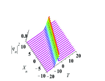
(a) Single bright soliton

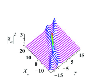
(b) Two bright soliton

Figure 1: (color online): Bright solitons

IV Single and multi-dark soliton solution

In this section, we construct the one- and multi-dark soliton solution for the defocusing CSP equation ($\sigma=-1$) in detail. Generally, the DT cannot apply to derive the dark solitons directly, since the spectral points of dark solitons locate in the real axis and the Darboux matrix is trivial if $\lambda_{1}=\lambda_{1}^{*}$. The authors in Ling develop a method to yield the dark soliton and multi-dark solitons through the Darboux transformation together with the limit technique. In what followings, we follow the steps in reference Ling to give the dark and multi-dark solitons for the semi-discrete CSP equation.

The dark solution and multi-dark solution can be constructed from the seed solution–plane wave solution through formula (35). We depart from the seed solution

$$\rho_{n}^{[0]}=\frac{\gamma}{2},\,\,q_{n}^{[0]}=\frac{\beta}{2}{\rm e}^{{\rm i}\theta_{n}},\,\,\theta_{n}=bn+\frac{c}{2}s,\,\,c=\frac{a\gamma}{2}\frac{\sin(b)}{\cos(b)-1},\,\,\gamma>0,\,\,\beta\geq 0,\,\,\,b\neq k\pi,\,\,k\in\mathbb{Z}.$$ (47)

Then we have the solution vector for Lax pair equation (17) with $(q_{n},\rho_{n};\lambda)=(q_{n}^{[0]},\rho_{n}^{[0]};\lambda_{i})$,

$$|y_{i,n}\rangle=KL_{i}E_{i}=K\begin{bmatrix}\widehat{\phi_{i,n}}\\ \beta\widehat{\psi_{i,n}}\\ \end{bmatrix},\,\,K=\mathrm{diag}\left({\rm e}^{-\frac{{\rm i}}{2}\theta_{n}},{\rm e}^{\frac{{\rm i}}{2}\theta_{n}}\right),\,\,\lambda_{i}\neq-c+{\rm i}\beta,$$ (48)

where $|y_{i,n}\rangle$ discards a function,

$$L_{i}=\begin{bmatrix}1&1\\[10.0pt] {\displaystyle\frac{\beta}{c+\chi_{i}^{+}}}&{\displaystyle\frac{\beta}{c+\chi_{i}^{-}}}\\ \end{bmatrix},\,\,E_{i}=\begin{bmatrix}{\rm e}^{\omega_{i,n}}\\ \alpha_{i}(\bar{\lambda_{i}}-\lambda_{i}){\rm e}^{-\omega_{i,n}}\\ \end{bmatrix}$$

and

$$\begin{split}\omega_{i,n}=&\frac{{\rm i}}{4}\xi_{i}s+\frac{n}{2}\ln\left({\frac{\sin(\frac{b}{2})\left(\frac{1}{2}{\rm i}a\gamma-\xi_{i}\right)+{\rm i}\cos(\frac{b}{2})\lambda_{i}}{\sin(\frac{b}{2})\left(\frac{1}{2}{\rm i}a{\gamma}+\xi_{i}\right)+{\rm i}\cos(\frac{b}{2})\lambda_{i}}}\right)+a_{i},\\ \chi_{i}^{\pm}=&\lambda_{i}\pm\xi_{i},\,\,\xi_{i}=\sqrt{(\lambda_{i}+c)^{2}-\beta^{2}}.\end{split}$$ (49)

$\alpha_{i}$s are appropriate complex parameters and $a_{i}$s are real parameters. In order to derive the single dark soliton solution, we consider only $\lambda_{1}$ and replace the parameter condition (49) with

$$\chi_{1}^{\pm}=\beta[\cos(\varphi_{1})\pm{\rm i}\sin(\varphi_{1})]\,\,,\xi_{1}={\rm i}\beta\sin(\varphi_{1}).$$ (50)

and $0<\varphi_{i}<\pi,$ $a_{i}\in\mathbf{R}$. By taking a limit process $\lambda_{1}\rightarrow\bar{\lambda}_{1}$ similar to the one in Ling , the single dark soliton solution can be obtained as follows

$$\begin{split}\rho_{n}^{[1]}=&\frac{\gamma}{2}+\frac{\beta}{2a}\sin(\varphi_{1})(\tanh(Z_{1,n+1})-\tanh(Z_{1,n})),\\ q_{n}^{[1]}=&\frac{\beta}{2}\left[1-{\rm i}\sin(\varphi_{1}){\rm e}^{-{\rm i}\varphi_{1}}-{\rm i}\sin(\varphi_{1}){\rm e}^{-{\rm i}\varphi_{1}}\tanh(Z_{1,n})\right]{\rm e}^{{\rm i}\theta_{n}},\\ x_{n}^{[1]}=&\frac{\gamma}{2}an+\frac{\beta^{2}}{8}s+\frac{\beta}{2a}\sin(\varphi_{1})\tanh(Z_{1,n}),\,\,t=-s,\end{split}$$ (51)

where

$$Z_{1,n}(\varphi_{1},a_{1})=\frac{n}{2}\ln\left(\frac{a\gamma+2\beta\sin(\frac{1}{2}b)\cos(\frac{1}{2}b+\varphi_{1})}{a\gamma+2\beta\sin(\frac{1}{2}b)\cos(\frac{1}{2}b-\varphi_{1})}\right)-\frac{\beta}{4}\sin(\varphi_{1})s+a_{1}.$$ (52)

and $a_{1}$ is a real parameter.

Next, we proceed to finding $N$-dark soliton solution. Based on the $N$-soliton solution (35) to the defocusing semi-discrete CSP equation, it then follows

$$\begin{split}q_{n}[N]=&\frac{\beta}{2}\left[1+\widehat{Y_{2,n}}M_{n}^{-1}\widehat{Y_{1,n}}^{{\dagger}}\right]\mathrm{e}^{\mathrm{i}\theta_{n}}=\frac{\beta}{2}\left[\frac{\det(H_{n})}{\det(M_{n})}\right]\mathrm{e}^{\mathrm{i}\theta_{n}},\\ x_{n}=&\frac{\gamma}{2}an+\frac{\beta^{2}}{8}s-\frac{2}{a}\ln_{s}(\det(M_{n})),\quad\,t=-s,\end{split}$$ (53)

where

$$\begin{split}M_{n}&=\left(\frac{\langle y_{i,n}|\sigma_{3}|y_{j,n}\rangle}{2(\bar{\lambda}_{i}-\lambda_{j})}\right)_{1\leq i,j\leq N},\quad\,H_{n}=M_{n}+Y_{1,n}^{{\dagger}}Y_{2,n},\\ \widehat{Y_{1,n}}&=\left[\widehat{\phi_{1,n}},\widehat{\phi_{2,n}},\cdots,\widehat{\phi_{N,n}}\right],\quad\,\widehat{Y_{2,n}}=\left[\widehat{\psi_{1,n}},\widehat{\psi_{2,n}},\cdots,\widehat{\psi_{N,n}}\right].\end{split}$$

In general, the above $N$-soliton solution (43) is singular. In order to derive the $N$-dark soliton solution through the DT method, we need to take a limit process $\lambda_{i}\rightarrow\bar{\lambda}_{i},(i=1,2,\cdots,N)$. By a tedious procedure which is omitted here, we finally have the $N$-dark soliton solution to the defocusing semi-discrete CSP equation (12) as follows

Proposition 3

$$\begin{split}\rho_{n}^{[N]}=&\frac{\gamma}{2}-\frac{2}{a}\ln_{s}\frac{\det(G_{n+1})}{\det(G_{n})},\\ q_{n}^{[N]}=&\frac{\beta}{2}\left[\frac{\det(H_{n})}{\det(G_{n})}\right]\mathrm{e}^{\mathrm{i}\theta_{n}},\\ x_{n}^{[N]}=&\frac{\gamma}{2}an+\frac{\beta^{2}}{8}s-\frac{2}{a}\ln_{s}\det(G_{n}),\,\,t=-s,\end{split}$$ (54)

where $G_{n}=(g_{i,j})_{1\leq i,j\leq N}$, $H_{n}=(h_{i,j})_{1\leq i,j\leq N}$,

$$\begin{split}g_{i,j}&=\frac{\delta_{ij}+\mathrm{e}^{Z_{i,n}+Z_{j,n}}}{\exp(-\mathrm{i}\varphi_{i})-\exp(\mathrm{i}\varphi_{j})},\\ h_{i,j}&=\frac{\delta_{ij}+\mathrm{e}^{(Z_{i,n}-\mathrm{i}\varphi_{i})+(Z_{j,n}-\mathrm{i}\varphi_{j})}}{\exp(-\mathrm{i}\varphi_{i})-\exp(\mathrm{i}\varphi_{j})},\end{split}$$ (55)

$Z_{i,n}=Z_{1,n}(\varphi_{i},a_{i})$ and $\delta_{i,j}$ is the standard Kronecker delta.

By taking $N=2$ in (54) and (55), the determinants corresponding to two-dark soliton solution can be calculated as

$$|G_{n}|=1+e^{2Z_{i,n}}+e^{2Z_{2,n}}+a_{12}e^{2(Z_{1,n}+Z_{2,n})}\,,$$ (56)

$$|H_{n}|=1+e^{2(Z_{i,n}-\mathrm{i}\varphi_{1})}+e^{2(Z_{2,n}-\mathrm{i}\varphi_{2})}+a_{12}e^{2(Z_{1,n}+Z_{2,n}-\mathrm{i}\varphi_{1}-\mathrm{i}\varphi_{2})}\,,$$ (57)

where

$$a_{12}=\frac{\sin^{2}\left(\frac{\varphi_{2}-\varphi_{1}}{2}\right)}{\sin^{2}\left(\frac{\varphi_{2}+\varphi_{1}}{2}\right)}\,.$$ (58)

Asymptotic analysis can be easily performed for two-soliton interaction, which shows that the collision is always elastic. We shows an example of such two-soliton collision. If we choose the parameter $a=1$, $\varphi_{1}=\arcsin(4/5)$ and $a_{1}=0$, then the single dark soliton are shown in Figure 2 (a). To shown their interaction for two dark solitons, choosing the parameters $a=1$, $\varphi_{1}=\arcsin(4/5)$, $\varphi_{2}=\pi/2$, $a_{1}=a_{2}=0$, we arrive at the dynamics of two dark solitons (Fig. 2(b)), which show that the interaction between them is elastic.

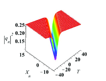
(a) Single dark soliton

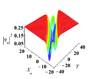
(b) Two dark soliton

Figure 2: (color online): Dark soliton.

Prior to the closing of this section, let us prove that the multi-dark solution converges to the its counterpart of the continuous CSP equation obtained in FenglingzhuPRE . In the continuous limit, we assume $a=b\to 0$, it then follows $c\to-\gamma$. Referring to the Taylor expansion (44), $Z_{i,n}$ turns out to be

$$\begin{split}&\frac{n}{2}\ln\left(\frac{a\gamma+2\beta\sin(\frac{1}{2}b)\cos(\frac{1}{2}b+\varphi_{i})}{a\gamma+2\beta\sin(\frac{1}{2}b)\cos(\frac{1}{2}b-\varphi_{i})}\right)-\frac{\beta}{4}\sin(\varphi_{i})s+a_{i}\\ &\approx n\frac{-2\beta\sin^{2}(\frac{b}{2})\sin(\varphi_{i})}{2\beta\cos(\frac{b}{2})\sin(\frac{b}{2})\cos(\varphi_{i})+a\gamma}-\frac{\beta}{4}\sin(\varphi_{i})s+a_{i}\,.\end{split}$$ (59)

Note that, between the present paper and FenglingzhuPRE $\gamma\to-\gamma$. As a result $Z_{i,n}\to\omega_{i}$ in FenglingzhuPRE by letting $nb=y$ and the proof is complete.

V Single breather and multi-breather solutions

The single breather and multi-breather solution for the focusing semi-discrete CSP equation (12) ($\sigma=1$) can be constructed from the seed solution–plane wave solution through formula (35). We depart from the seed solution

$$\rho_{n}^{[0]}=\frac{\gamma}{2},\,\,q_{n}^{[0]}=\frac{\beta}{2}\mathrm{e}^{\mathrm{i}\theta_{n}},\,\,\theta_{n}=bn+\frac{c}{2}s,\,\,c=\frac{a\gamma}{2}\frac{\sin(b)}{\cos(b)-1},\,\,\gamma>0,\,\,\beta\geq 0.$$ (60)

The coordinates for semi-discrete CSP (12) can be obtained

$$x_{n}(s)=\frac{\gamma}{2}na-\frac{\beta^{2}}{8}s,\,\,t=-s.$$

Then we have the solution vector for Lax pair equation (17) ($\sigma=1$) with$(q_{n},\rho_{n};\lambda)=(q_{n}^{[0]},\rho_{n}^{[0]};\lambda_{1})$,

$$|y_{1,n}\rangle=KL_{1}E_{1},\,\,K=\mathrm{diag}\left(\mathrm{e}^{-\frac{\mathrm{i}}{2}\theta_{n}},\mathrm{e}^{\frac{\mathrm{i}}{2}\theta_{n}}\right),\,\,\lambda_{1}\neq-c+\mathrm{i}\beta,$$ (61)

where

$$L_{1}=\begin{bmatrix}1&1\\[10.0pt] {\displaystyle\frac{\beta}{c+\eta_{1}}}&{\displaystyle\frac{\beta}{c+\chi_{1}}}\end{bmatrix},\,\,E_{i}=\begin{bmatrix}\mathrm{e}^{\theta_{1,n}}\\ 1\\ \end{bmatrix}$$

and

$$\begin{split}\theta_{1,n}=&\frac{\mathrm{i}}{2}\xi_{1}s+n\ln\left({\frac{\sin(\frac{b}{2})\left(\frac{1}{2}\mathrm{i}a\gamma-\xi_{1}\right)+\mathrm{i}\cos(\frac{b}{2})\lambda_{1}}{\sin(\frac{b}{2})\left(\frac{1}{2}\mathrm{i}a{\gamma}+\xi_{1}\right)+\mathrm{i}\cos(\frac{b}{2})\lambda_{1}}}\right)+a_{1},\\ \eta_{1}=&\lambda_{1}+\xi_{1},\,\,\chi_{1}=\lambda_{1}-\xi_{1},\,\,\xi_{1}=\sqrt{\beta^{2}+(\lambda_{1}+c)^{2}}.\end{split}$$ (62)

The single breather solution can be constructed from the formula (35) with the technique as in reference Ling :

$$\begin{split}\rho_{n}^{[1]}=&\frac{\gamma}{2}-\frac{2}{a}\ln_{s}\left(\frac{\cosh(\theta_{1,n+1}^{R})\cosh(\varphi_{1}^{R}/2)-\sin(\theta_{1,n+1}^{I})\sin(\varphi_{1}^{I}/2)}{\cosh(\theta_{1,n}^{R})\cosh(\varphi_{1}^{R}/2)-\sin(\theta_{1,n}^{I})\sin(\varphi_{1}^{I}/2)}\right)>0,\\ q_{n}^{[1]}=&\frac{\beta}{2}\left[\frac{\cosh(\theta_{1,n}^{R}-\mathrm{i}\varphi_{1}^{I})\cosh(\varphi_{1}^{R}/2)+\sin(\theta_{1,n}^{I}+\mathrm{i}\varphi_{1}^{R})\sin(\varphi_{1}^{I}/2)}{\cosh(\theta_{1,n}^{R})\cosh(\varphi_{1}^{R}/2)-\sin(\theta_{1,n}^{I})\sin(\varphi_{1}^{I}/2)}\right]\mathrm{e}^{\mathrm{i}\theta_{n}},\\ x_{n}^{[1]}=&\frac{\gamma}{2}na-\frac{\beta^{2}}{8}s-\frac{2}{a}\ln_{s}\left(\cosh(\theta_{1,n}^{R})\cosh(\varphi_{1}^{R}/2)-\sin(\theta_{1,n}^{I})\sin(\varphi_{1}^{I}/2)\right),\,\,t=-s,\end{split}$$ (63)

where

$$\xi_{i}=\beta\cosh\left[\frac{1}{2}(\varphi_{i}^{R}+\mathrm{i}\varphi_{i}^{I})\right],\,\,\eta_{i}+c=\beta\mathrm{e}^{\frac{1}{2}(\varphi_{i}^{R}+\mathrm{i}\varphi_{i}^{I})},\,\,\chi_{i}+c=-\beta\mathrm{e}^{-\frac{1}{2}(\varphi_{i}^{R}+\mathrm{i}\varphi_{i}^{I})}.$$

$$\begin{split}\theta_{1,n}^{R}&=\frac{\ln(g_{1})}{2}n-\frac{\beta}{2}\sinh\left(\frac{\varphi_{1}^{R}}{2}\right)\sin\left(\frac{\varphi_{1}^{I}}{2}\right)s-\varphi_{1}^{R}+a_{1}^{R},\\ \theta_{1,n}^{I}&=h_{1}n+\frac{\beta}{2}\cosh\left(\frac{\varphi_{1}^{R}}{2}\right)\cos\left(\frac{\varphi_{1}^{I}}{2}\right)s-\varphi_{1}^{I}+a_{1}^{I},\end{split}$$

and

$$\begin{split}g_{1}&=\frac{\beta^{2}\cosh^{2}\left(\varphi_{1}^{R}/2\right)\sin^{2}\left(b/2+\varphi_{1}^{I}/2\right)+\left[\beta\sinh\left(\varphi_{1}^{R}/2\right)\cos\left(b/2+\varphi_{1}^{I}/2\right)+\frac{a\gamma}{2\sin\left(b/2\right)}\right]^{2}}{\beta^{2}\cosh^{2}\left(\varphi_{1}^{R}/2\right)\sin^{2}\left(b/2-\varphi_{1}^{I}/2\right)+\left[\beta\sinh\left(\varphi_{1}^{R}/2\right)\cos\left(b/2-\varphi_{1}^{I}/2\right)+\frac{a\gamma}{2\sin\left(b/2\right)}\right]^{2}},\\ h_{1}&=\mathrm{arg}\left({\frac{\sin(\frac{b}{2})\left(\frac{1}{2}\mathrm{i}a\gamma-\beta\cosh\left[\frac{1}{2}(\varphi_{1}^{R}+\mathrm{i}\varphi_{1}^{I})\right]\right)+\mathrm{i}\cos(\frac{b}{2})(\beta\sinh\left[\frac{1}{2}(\varphi_{1}^{R}+\mathrm{i}\varphi_{1}^{I})\right]-c)}{\sin(\frac{b}{2})\left(\frac{1}{2}\mathrm{i}a{\gamma}+\beta\cosh\left[\frac{1}{2}(\varphi_{1}^{R}+\mathrm{i}\varphi_{1}^{I})\right]\right)+\mathrm{i}\cos(\frac{b}{2})(\beta\sinh\left[\frac{1}{2}(\varphi_{1}^{R}+\mathrm{i}\varphi_{1}^{I})\right]-c)}}\right).\end{split}$$

Specially, if we choose the parameters such that $\beta=\gamma=1$, $a=2$, $b=\frac{\pi}{2}$, $\varphi_{1R}=0$, $\varphi_{1I}=\arcsin(\frac{3}{5})$, $a_{1}=0$, we can obtain the explicit dynamics (Fig. 3(a)) for the breather solution which is periodical in time and localized in space and usually is called the Kuznetsov-Ma (K-M) breather.

Furthermore, by using the generalized $N$-fold DT, we drive the $N$-breather solution through the formula (35) and some tedious algebraic calculations as the following proposition

Proposition 4

The multi-breather solution for semi-discrete CSP equation (12) can be represented as

$$\begin{split}\rho_{n}^{[N]}&=\frac{\gamma}{2}-\frac{2}{a}\ln_{s}\left(\frac{\det(M_{n+1})}{\det(M_{n})}\right),\\ q_{n}^{[N]}&=\frac{\beta}{2}\left[\frac{\det(G_{n})}{\det(M_{n})}\right]\mathrm{e}^{\mathrm{i}\theta_{n}},\\ x_{n}^{[N]}&=\frac{\gamma}{2}an-\frac{\beta^{2}}{8}s-\frac{2}{a}\ln_{s}\det(M_{n}),\,\,t=-s,\end{split}$$ (64)

where

$$\begin{split}M_{n}&=\left(\frac{\mathrm{e}^{\theta_{m,n}^{\ast}+\theta_{k,n}}}{\eta_{m}^{\ast}-\eta_{k}}-\frac{\mathrm{e}^{\theta_{m,n}^{\ast}}}{\eta_{m}^{\ast}-\chi_{k}}-\frac{\mathrm{e}^{\theta_{k,n}}}{\chi_{m}^{\ast}-\eta_{m}}+\frac{1}{\chi_{m}^{\ast}-\chi_{k}}\right)_{1\leq m,k\leq N},\,\,\\ G_{n}&=\left(\frac{\mathrm{e}^{\theta_{m,n}^{\ast}+\theta_{k,n}}}{\eta_{m}^{\ast}-\eta_{k}}\frac{\eta_{m}^{\ast}+c}{\eta_{k}+c}-\frac{\mathrm{e}^{\theta_{m,n}^{\ast}}}{\eta_{m}^{\ast}-\chi_{k}}\frac{\eta_{m}^{\ast}+c}{\chi_{k}+c}-\frac{\mathrm{e}^{\theta_{k,n}}}{\chi_{m}^{\ast}-\eta_{m}}\frac{\chi_{m}^{\ast}+c}{\eta_{k}+c}+\frac{1}{\chi_{m}^{\ast}-\chi_{k}}\frac{\chi_{m}^{\ast}+c}{\chi_{k}+c}\right)_{1\leq m,k\leq N},\end{split}$$

the parameters $\theta_{k,n}$, $\eta_{i}$, $\chi_{i}$ are given in equations (49).

Finally, we provide a proof that the above multi-breather solution will converge to the multi-breather solution to the CSP equation obtained in LFZPhysD . To this end, we assume $a=b\to 0$ in the continuous limit and notice that $\gamma\to-\gamma$ in compared with the dark soliton solution in LFZPhysD . By using the Taylor expansion (44), $\theta_{i,n}$ becomes

$$\begin{split}&\frac{\mathrm{i}}{2}\xi_{i}s+n\ln\left({\frac{\sin(\frac{b}{2})\left(\frac{1}{2}\mathrm{i}a\gamma-\xi_{i}\right)+\mathrm{i}\cos(\frac{b}{2})\lambda_{i}}{\sin(\frac{b}{2})\left(\frac{1}{2}\mathrm{i}a{\gamma}+\xi_{i}\right)+\mathrm{i}\cos(\frac{b}{2})\lambda_{i}}}\right)+a_{i}\\ &\approx\frac{\mathrm{i}}{2}\xi_{i}s-2n\frac{\sin(\frac{b}{2})\xi_{i}}{\mathrm{i}\cos(\frac{b}{2})\lambda_{i}+\frac{1}{2}\mathrm{i}a\gamma\sin(\frac{b}{2})}+a_{i}\\ &=\frac{\mathrm{i}}{2}\xi_{i}s+\frac{\mathrm{i}\xi_{i}}{\lambda_{i}}y+a_{i}\end{split}$$ (65)

by letting $nb=y$ in the continuous limit $b\to 0$. This shows how the multi-breather solution to semi-discrete CSP equation converges to the multi-breather solution of the CSP equation in the continuous limit.

VI Fundamental and high-order rogue wave solution

In this section, we will derive the general rogue wave solution for the focusing semi-discrete CSP equation based on the general breather solution obtained in the previous section. Since the solution vectors involve the square root of a complex number, it is inconvenient to calculate. To avoid this trouble, we introduce the following transformation:

$$\lambda_{i}+c=\beta\sinh\left[\frac{1}{2}(\varphi_{i}^{R}+\mathrm{i}\varphi_{i}^{I})\right],\,\,(\varphi_{i}^{R},\varphi_{i}^{I})\in\Omega,$$

where $\Omega=\{(\varphi^{R},\varphi^{I})|0<\varphi^{I}<\pi,\,\text{and }0<\varphi^{R}<\infty,\text{or }\varphi^{R}=0,\text{and }\frac{\pi}{2}\leq\varphi^{I}<\pi\}$, then

$$\xi_{i}=\beta\cosh\left[\frac{1}{2}(\varphi_{i}^{R}+\mathrm{i}\varphi_{i}^{I})\right],\,\,\eta_{i}+c=\beta\mathrm{e}^{\frac{1}{2}(\varphi_{i}^{R}+\mathrm{i}\varphi_{i}^{I})},\,\,\chi_{i}+c=-\beta\mathrm{e}^{-\frac{1}{2}(\varphi_{i}^{R}+\mathrm{i}\varphi_{i}^{I})}.$$

Actually, we can obtain the rogue wave solution and high order rogue wave solutions in this special point. The general procedure to yield these solutions was proposed in Guo1 ; Guo2 . If we solve the linear system (17) with $(q_{n},\rho_{n},\lambda)=(q_{n}^{[0]},\rho_{n}^{[0]},-c+\mathrm{i}\beta)$, where $q_{n}^{[0]}$ and $\rho_{n}^{[0]}$ are given in equations (47), then the quasi-rational solution vector is obtained. With this solution vector, we could construct the first order rogue wave solution but fails to obtain the high order RW solutions. To obtain the general high order rogue wave solution with a simple way, we must solve the linear system (17) with $(q_{n},\rho_{n},\lambda)=(q_{n}^{[0]},\rho_{n}^{[0]},-c+\mathrm{i}\beta\cos(\epsilon))$, where $\epsilon$ is a small parameter. Denote

$$\lambda_{1}=-c+\mathrm{i}\beta\cos(\epsilon),\,\,\xi_{1}=\beta\sin(\epsilon),\,\,\eta_{1}=\lambda_{1}+\xi_{1}=-c+\mathrm{i}\beta\mathrm{e}^{-\mathrm{i}\epsilon},\,\,c=-\frac{1}{2}a\gamma\cot(\frac{b}{2}).$$ (66)

Lemma 1

The following parameters can be expanded with $\epsilon$, where $\epsilon$ is a small parameter

$$\begin{split}\mu_{1}&=\sum_{n=0}^{\infty}\mu_{1}^{[n]}\epsilon^{2n+1},\\ \frac{\beta}{\mathrm{i}(\eta_{1}^{*}-\eta_{1})}&=\frac{1}{\mathrm{e}^{\mathrm{i}\epsilon^{*}}+\mathrm{e}^{-\mathrm{i}\epsilon}}=\sum_{i=0,j=0}^{\infty,\infty}F^{[i,j]}\epsilon^{*i}\epsilon^{j},\end{split}$$

where

$$\begin{split}\mu_{1}^{[n]}&=\frac{\beta\left(-1\right)^{n}}{(2n+1)!},\\ F^{[i,j]}&=\frac{1}{i!j!}\frac{\partial^{i+j}}{\partial\epsilon^{*i}\partial\epsilon^{j}}\left(\left[\mathrm{e}^{\mathrm{i}\epsilon^{*}}+\mathrm{e}^{-\mathrm{i}\epsilon}\right]^{-1}\right)_{|_{\epsilon^{*}=0,\epsilon=0}},\end{split}$$

With the aid of above lemma 1, we obtain the following expansion

$$\begin{split}Z_{1,n}&\equiv\frac{\mathrm{i}\beta}{4}\sin\left(\epsilon\right)s+\frac{n}{2}\ln\left({\frac{\beta\sin\left(\frac{3}{2}b-\epsilon\right)+\beta\sin\left(\frac{1}{2}b+\epsilon\right)-2\mathrm{i}\cos\left(\frac{1}{2}b\right)a{\gamma}}{\beta\sin\left(\frac{3}{2}b+\epsilon\right)+\beta\sin\left(\frac{1}{2}b-\epsilon\right)-2\mathrm{i}\cos\left(\frac{1}{2}b\right)a{\gamma}}}\right)-\frac{\mathrm{i}\epsilon}{2}+\sum_{i=1}^{\infty}(e_{i}+\mathrm{i}f_{i})\epsilon^{2i-1},\\ &=\mathrm{i}\epsilon\sum_{k=0}^{\infty}Z_{1,n}^{[2k+1]}\epsilon^{2k},\end{split}$$

where

$$Z_{1,n}^{[2k+1]}=\frac{\mathrm{d}^{2k+1}}{\mathrm{d}\epsilon^{2k+1}}Z_{1,n}|_{\epsilon=0}.$$

Furthermore we have

$$\mathrm{e}^{Z_{1,n}}=\sum_{i=0}^{\infty}S_{i}(\mathbf{Z}_{1,n})\epsilon^{i},\,\,\mathbf{Z}_{1,n}=\left(Z_{1,n}^{[1]},Z_{1,n}^{[2]},\cdots\right),\,\,Z_{1,n}^{[2k]}=0,\,\,k\geq 1\\$$

the explicit expression of these polynomials can be are given by the elementary Schur polynomials

$$\begin{split}S_{0}(\mathbf{Z}_{1,n})=&1,\,\,S_{1}(\mathbf{Z}_{1,n})=Z_{1,n}^{[1]},\,\,S_{2}(\mathbf{Z}_{1,n})=Z_{1,n}^{[2]}+\frac{(Z_{1,n}^{[1]})^{2}}{2},\,\,S_{3}(\mathbf{Z}_{1,n})=Z_{1,n}^{[3]}+Z_{1,n}^{[1]}Z_{1,n}^{[2]}+\frac{(Z_{1,n}^{[1]})^{3}}{6},\cdots\\ S_{i}(\mathbf{Z}_{1,n})=&\sum_{l_{1}+2l_{2}+\cdots+kl_{k}=i}\frac{(Z_{1,n}^{[1]})^{l_{1}}(Z_{1,n}^{[2]})^{l_{2}}\cdots(Z_{1,n}^{[k]})^{l_{k}}}{l_{1}!l_{2}!\cdots l_{k}!}.\end{split}$$

Since $KE_{1,n}(\epsilon)$ satisfies the Lax equation (17), then $KE_{1,n}(-\epsilon)$ also satisfies the Lax equation (17). To obtain the general high order rogue wave solution, we choose the general special solution

$$|y_{1,n}\rangle=\frac{K}{2\epsilon}\left[E_{1,n}(\epsilon)-E_{1,n}(-\epsilon)\right]\equiv K\begin{bmatrix}\varphi_{1,n}\\[8.0pt] \beta\psi_{1,n}\\ \end{bmatrix},$$

where

$$E_{1,n}=\begin{bmatrix}\mathrm{e}^{Z_{1,n}}\\ {\displaystyle\frac{\beta\mathrm{e}^{Z_{1,n}}}{\eta_{1}+c}}\\ \end{bmatrix},$$

Finally, we have

$$\begin{split}\frac{\beta\langle y_{1,n}|y_{1,n}\rangle}{2\mathrm{i}(\lambda_{1}^{*}-\lambda_{1})}&=\frac{\beta}{4\mathrm{i}}\left[\frac{\mathrm{e}^{Z_{1,n}^{*}+Z_{1,n}}}{\eta_{1}^{*}-\eta_{1}}-\frac{\mathrm{e}^{Z_{1,n}^{*}-Z_{1,n}}}{\eta_{1}^{*}-\chi_{1}}-\frac{\mathrm{e}^{-Z_{1,n}^{*}+Z_{1,n}}}{\chi_{1}^{*}-\eta_{1}}+\frac{\mathrm{e}^{-Z_{1,n}^{*}-Z_{1,n}}}{\chi_{1}^{*}-\chi_{1}}\right]\\ &=\sum_{m=1,k=1}^{\infty,\infty}M_{n}^{[m,k]}{\epsilon}^{*2(m-1)}\epsilon^{2(k-1)}\end{split}$$ (67)

and

$$\begin{split}&\frac{\mathrm{i}\beta\langle y_{1,n}|y_{1,n}\rangle}{2(\lambda_{1}^{*}-\lambda_{1})}+\mathrm{i}\beta\varphi_{1,n}\psi_{1,n}\\ =&\frac{\mathrm{i}\beta}{4}\left[\frac{\mathrm{e}^{Z_{1,n}^{*}+Z_{1,n}}}{\eta_{1}^{*}-\eta_{1}}\frac{\eta_{1}^{*}+c}{\eta_{1}+c}-\frac{\mathrm{e}^{Z_{1,n}^{*}-Z_{1,n}}}{\eta_{1}^{*}-\chi_{1}}\frac{\eta_{1}^{*}+c}{\chi_{1}+c}-\frac{\mathrm{e}^{-Z_{1,n}^{*}+Z_{1,n}}}{\chi_{1}^{*}-\eta_{1}}\frac{\chi_{1}^{*}+c}{\eta_{1}+c}+\frac{\mathrm{e}^{-Z_{1,n}^{*}-Z_{1,n}}}{\chi_{1}^{*}-\chi_{1}}\frac{\chi_{1}^{*}+c}{\chi_{1}+c}\right]\\ =&\sum_{m=1,k=1}^{\infty,\infty}G_{n}^{[m,k]}{\epsilon}^{*2(m-1)}\epsilon^{2(k-1)}\end{split}$$ (68)

where $\chi_{1}=\eta_{1}(-\epsilon),$

$$\begin{split}M_{n}^{[m,k]}&=\sum_{i=0}^{2m-1}\sum_{j=0}^{2k-1}F^{[i,j]}S_{2k-i-1}(\mathbf{Z}_{1,n})S_{2m-j-1}(\mathbf{Z}_{1,n}^{*}),\\ G_{n}^{[m,k]}&=\sum_{i=0}^{2m-1}\sum_{j=0}^{2k-1}F^{[i,j]}S_{2k-i-1}(\mathbf{Z}_{1,n}+\mathbf{\varepsilon})S_{2m-j-1}(\mathbf{Z}_{1,n}^{*}+\mathbf{\varepsilon}),\end{split}$$ (69)

and $\mathbf{\varepsilon}=(1,0,0,\cdots).$

Based on the expansion equations (67)-(68), and formulas (35)-(38), we can obtain the general rogue wave solutions:

Proposition 5

The general high order rogue wave solution for semi-discrete CSP equation (12) can be represented as

$$\begin{split}\rho_{n}^{[N]}&=\frac{\gamma}{2}-\frac{2}{a}\ln_{s}\left(\frac{\det(M_{n+1})}{\det(M_{n})}\right)>0,\\ q_{n}^{[N]}&=\frac{\beta}{2}\left[\frac{\det(G_{n})}{\det(M_{n})}\right]\mathrm{e}^{\mathrm{i}\theta_{n}},\\ x_{n}^{[N]}&=\frac{\gamma}{2}an-\frac{\beta^{2}}{8}s-\frac{2}{a}\ln_{t}\det(M_{n}),\,\,t=-s,\end{split}$$ (70)

where

$$M_{n}=\left(M_{n}^{[m,k]}\right)_{1\leq m,k\leq N},\,\,G_{n}=\left(G_{n}^{[m,k]}\right)_{1\leq m,k\leq N},$$

the expressions $M_{n}^{[m,k]}$ and $G_{n}^{[m,k]}$ are given in equations (69).

Specially, the first order rogue wave solution can be written explicitly through formula (70)

$$\begin{split}\rho_{n}^{[1]}=&\frac{\gamma}{2}-\frac{2}{a}\ln_{s}\left(\frac{\frac{1}{4}+(Z_{n+1,R}^{[1]})^{2}+(Z_{n+1,I}^{[1]}+\frac{1}{2})^{2}}{\frac{1}{4}+(Z_{n,R}^{[1]})^{2}+(Z_{n,I}^{[1]}+\frac{1}{2})^{2}}\right),\\ q_{n}^{[1]}=&\frac{\beta}{2}\left[1-\frac{1-2\mathrm{i}Z_{n,R}^{[1]}}{\frac{1}{4}+(Z_{n,R}^{[1]})^{2}+(Z_{n,I}^{[1]}+\frac{1}{2})^{2}}\right]\mathrm{e}^{\mathrm{i}\theta},\\ x_{n}^{[1]}=&\frac{\gamma}{2}an-\frac{\beta^{2}}{8}s-\frac{2}{a}\ln_{s}\left(\frac{1}{4}+(Z_{n,R}^{[1]})^{2}+(Z_{n,I}^{[1]}+\frac{1}{2})^{2}\right),\,\,t=-s,\end{split}$$

where

$$\begin{split}Z_{n,R}^{[1]}=&\frac{4{\beta}^{2}\sin^{3}(\frac{b}{2})\cos(\frac{b}{2})n}{{a}^{2}{\gamma}^{2}+2{\ \beta}^{2}\sin^{2}(b)},\\ Z_{n,I}^{[1]}=&\beta\left(\frac{2a\gamma\sin^{2}(\frac{b}{2})n}{{a}^{2}{\gamma}^{2}+2{\ \beta}^{2}\sin^{2}(b)}+\frac{s}{4}\right)-\frac{1}{2}.\end{split}$$ (71)

Moreover, the general second order rogue wave solution can be represented by the formula (70):

$$\begin{split}\rho_{n}^{[2]}=&\frac{\gamma}{2}-\frac{2}{a}\ln_{s}\left(\frac{F_{1,n+1}+\mathrm{i}F_{2,n+1}}{F_{1,n}+\mathrm{i}F_{2,n}}\right)>0,\\ q_{n}^{[2]}=&\frac{\beta}{2}\left[1+\frac{G_{n}}{F_{1,n}+\mathrm{i}F_{2,n}}\right]\mathrm{e}^{\mathrm{i}\theta_{n}},\\ x_{n}^{[2]}=&\frac{\gamma}{2}an-\frac{\beta^{2}}{8}s-\frac{2}{a}\ln_{s}\left(F_{1,n}+\mathrm{i}F_{2,n}\right),\,\,t=-s,\end{split}$$

where

$$\begin{split}F_{1,n}=&\left(-{\frac{1}{72}}\overline{Z_{n}^{[1]}}-\frac{1}{12}\overline{Z_{n}^{[3]}}+\frac{1}{36}{\overline{Z_{n}^{[1]}}}^{3}\right)({Z_{n}^{[1]}})^{3}+\left(\frac{1}{8}{\overline{Z_{n}^{[1]}}}^{2}-{\frac{1}{64}}\right)({Z_{n}^{[1]}})^{2}+\left(-{\frac{1}{72}}{\overline{Z_{n}^{[1]}}}^{3}+\frac{1}{24}\overline{Z_{n}^{[3]}}+{\frac{29}{288}}\overline{Z_{n}^{[1]}}\right)Z_{n}^{[1]}\\ &+\frac{1}{4}Z_{n}^{[3]}\overline{Z_{n}^{[3]}}-\frac{1}{12}Z_{n}^{[3]}{\overline{Z_{n}^{[1]}}}^{3}-{\frac{1}{64}}{\overline{Z_{n}^{[1]}}}^{2}+\frac{1}{24}\overline{Z_{n}^{[1]}}Z_{n}^{[3]}+{\frac{1}{64}},\end{split}$$

$$F_{2,n}=\frac{1}{24}{Z_{n}^{[1]}}^{2}{\overline{Z_{n}^{[1]}}}^{3}+\frac{1}{8}{\overline{Z_{n}^{[1]}}}^{2}Z_{n}^{[3]}-\frac{1}{24}{\overline{Z_{n}^{[1]}}}^{2}{Z_{n}^{[1]}}^{3}-\frac{1}{8}{Z_{n}^{[1]}}^{2}\overline{Z_{n}^{[3]}}+\frac{1}{12}Z_{n}^{[1]}{\overline{Z_{n}^{[1]}}}^{2}-\frac{1}{12}{Z_{n}^{[1]}}^{2}\overline{Z_{n}^{[1]}}+\frac{1}{32}\overline{Z_{n}^{[1]}}-\frac{1}{32}Z_{n}^{[1]},$$

$$\begin{split}G_{n}=&\frac{1}{12}\mathrm{i}{\overline{Z_{n}^{[1]}}}^{2}{Z_{n}^{[1]}}^{3}+\left(\frac{1}{12}\mathrm{i}\overline{Z_{n}^{[1]}}-\frac{1}{4}{\overline{Z_{n}^{[1]}}}^{2}-\frac{1}{4}\mathrm{i}\overline{Z_{n}^{[3]}}+\frac{1}{12}\mathrm{i}{\overline{Z_{n}^{[1]}}}^{3}\right){Z_{n}^{[1]}}^{2}+\left(\frac{1}{2}\overline{Z_{n}^{[3]}}-\frac{1}{6}{\overline{Z_{n}^{[1]}}}^{3}-\frac{1}{6}\mathrm{i}{\overline{Z_{n}^{[1]}}}^{2}-\frac{1}{6}\overline{Z_{n}^{[1]}}\right)Z_{n}^{[1]}\\ &-\frac{1}{4}\mathrm{i}{\overline{Z_{n}^{[1]}}}^{2}Z_{n}^{[3]}+\frac{1}{4}\mathrm{i}\overline{Z_{n}^{[3]}}-\frac{1}{12}\mathrm{i}\overline{Z_{n}^{[1]}}-\frac{1}{12}\mathrm{i}{\overline{Z_{n}^{[1]}}}^{3},\end{split}$$

$Z_{n}^{[1]}=Z_{n,R}^{[1]}+\mathrm{i}Z_{n,I}^{[1]}$, the symbol overbar denotes the complex conjugation and

$$Z_{n}^{[3]}=\frac{\frac{2}{3}\mathrm{i}\beta\sin^{2}(\frac{1}{2}b)\left(2a\beta\gamma\sin(b)+\mathrm{i}{a}^{2}\gamma^{2}+8\mathrm{i}{\ \beta}^{2}\sin^{2}(\frac{1}{2}b)\right)}{2\beta{a}^{2}{\gamma}^{2}\sin(b)-{\beta}^{3}\sin^{3}(b)-\mathrm{i}{a}^{3}{\gamma}^{3}+3\mathrm{i}a\beta^{2}\gamma\sin^{2}(b)}\frac{n}{2}-\frac{\mathrm{i}\beta s}{24}+(e_{1}+f_{1}\mathrm{i}).$$

To illustrate the dynamics of rogue waves, we firstly show the fundamental rogue wave in Fig. 3(b) with the parameters $a=2$, $b=\frac{\pi}{2}$, $\beta=1$, $\gamma=\frac{5}{4}$. For the second order rogue waves, we firstly choose the parameters $a=2$, $b=\frac{\pi}{2}$, $\beta=1$, $\gamma=\frac{5}{2}$, $e_{1}=f_{1}=0$, then the standard second order RWs is shown in Fig. 4 (a). To exhibit the other dynamics for the second order RWs, we choose the parameters $a=2$, $b=\frac{\pi}{2}$, $\beta=1$, $\gamma=\frac{3}{2}$, $e_{1}=10$, $f_{1}=0$. It is seen that the temporal-spatial distribution exhibit the triangle shape as shown in Fig. 4 (b).

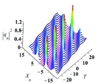
(a) K-M breather

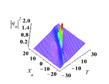
(b) Fundamental RW

Figure 3: (color online): Breather and Rogue waves

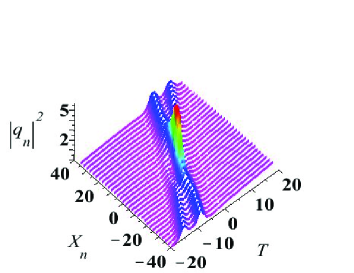
(a) Second order RW

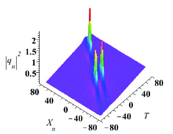
(b) Second order RW

Figure 4: (color online): Second order rogue waves with different dynamics

We remark here that since the higher order rogue wave solution is obtained from multi-breather solution to the semi-discrete CSP equation which converges to its counterpart in the continuous CSP equation, thus, the high order rogue wave solution for the semi-discrete CSP equation should converge to the one for CSP equation in the continuous limit.

VII Conclusions and discussions

In the present paper, we firstly drive the generalized Darbourx transformation (gDT) for the semi-discrete CSP equation (12) with the aid of discrete hodograph transformation. Based on formulas derived from the gDT, we then construct the multi-bright soliton solution for the focusing CSP equation with zero boundary condition. For the nonzero boundary conditions, we construct the multi-dark soliton solution for the defocusing case, the multi-breather solution and high-order rogue wave solution for the focusing case. We require the condition $\rho_{n}>0$ to keep the non-singularity and monodromy. Otherwise, if $\rho_{n}$ does not keep the positive definitive property, then the cusp or loop soliton would appear. All above solutions are shown to converge to their counterparts for the original CSP equation in the continuous limit.

It is noticed that a robust inverse scattering transform method has been proposed for the NLS equation by appropriately setting up and solving the Riemann-Hilbert problemBP ; BLM . It is imperative to study the inverse scattering transform and Riemann-Hilbert problem for both the original and semi-discrete CSP equation. Although the multi-bright soliton solutions have been constructed by Hirota’s bilinear method in determinant form FMO-PJMI and in pfaffian form FMOmultiSP , it would be interesting to drive other types of solutions such as dark-soliton, breather and rogue wave solutions for the semi-discrete CSP equation.

In the last, we should point out the following coupled semi-discrete CSP equation

$$\begin{split}&\frac{d}{dt}(q_{1,n+1}-q_{1,n})=\frac{1}{2}(x_{n+1}-x_{n})(q_{1,n+1}+q_{1,n}),\\ &\frac{d}{dt}(q_{2,n+1}-q_{2,n})=\frac{1}{2}(x_{n+1}-x_{n})(q_{2,n+1}+q_{2,n}),\\ &\frac{d}{dt}(x_{n+1}-x_{n})+\frac{1}{2}\sum_{j=1}^{2}\sigma_{j}\left(|q_{j,n+1}|^{2}-|q_{j,n}|^{2}\right)=0\,,\end{split}$$ (72)

which has been shown to be integrable recently FMOmultiSP . Beside the multi-bright soliton solution implied in FMOmultiSP , how about its general initial value problem and other types of soliton solutions?

The method provided in this paper is also useful to the coupled semi-discrete CSP equation. We expect to obtain and report the results in the near future. As the last conment, The obtained semi-discrete equations can be served as superior numerical schemes: the so-called self-adaptive moving mesh schemes for the CSP and coupled CSP equations.

References

• (1) S., Donna, M., Gerard, Compression of amplified chirped optical pulses, Optics Commun., 56 219?221 (1985).
• (2) G. P. Agrawal, Nonlinear Fiber Optics, (Academic Press, New York, 1995).
• (3) A. Hasegawa and Y. Kodama, Solitons in Optical Communications, (Clarendon, Oxford, 1995).
• (4) Y S. Kivshar, G. P. Agrawal, optical Solitons: From Fibers to Photonic Crystals, (Academic Press, San Diego, 2003).
• (5) A. Hasegawa and F. Tappert, Transmission of stationary nonlinear optical pulses in dispersive dielectric fibers I. Anomolous dispersion, Appl. Phys. Lett. 23 142 (1973).
• (6) A. Hasegawa and F. Tappert, Transmission ofstationary nonlinear optical pulses in dispersive dielectric fibers II. Normal dispersion, Appl. Phys. Lett. 23 171 (1973).
• (7) M. J. Ablowitz, P. A.  Clarkson, Solitons, Nonlinear Evolution Equations and Inverse Scattering (London Mathematical Society Lecure Notes Series 149), (Cambridge Univ. Press, Cambridge, 1991).
• (8) M. J. Ablowitz, B. Prinari, and A. D. Trubatch, Discrete and continuous nonlinear Schrödinger systems, (Cambridge Univ. Press, Cambridge, 2004).
• (9) F. Dalfovo, S. Giorgini and L. P.  Stringari, Theory of Bose-Einstein condensation in trapped gases, Rev. Mod. Phys. 71 463–512 (1999).
• (10) D. J. Benney and A. C. Newell, The propagation ofnonlinear wave envelopes, Stud. Appl. Math. 46 133–139 (1967).
• (11) V. E. Zakharov, Collapse of Langumuir waves, Sov. Phys. JETP 35 908–914 (1972).
• (12) V. E. Zakharov and A. B. Shabat, Exact theory of two-dimensional self-focusing and one-dimensional self-modulations of waves in nonlinear media, Sov. Phys. JETP 34 62–69 (1972).
• (13) V. E. Zakharov and A. B. Shabat, Interaction betweem solitons in a stable medium, Sov. Phys. JETP 37 823–828 (1973).
• (14) D. Krokel, N. J. Halas, G. Giuliani and D. Grischkowsky, Dark-pulse propagation in optical fibers, Phys. Rev. Lett. 60 29 (1988).
• (15) A. M. Weiner, J. P. Heritage, R. J. Hawkins, R. N. Thurston, E. M. Kirschner, D. E. Leaird and W. J. Tomlinson, Experimental observation of the fundamental dark soliton in optical fibers, Phys. Rev. Lett. 61 2445 (1988).
• (16) O. R. Solli, C. Ropers, P. Koonath, B. Jalali, Optical rogue waves, Nature, 450 1054–1057 (2007).
• (17) B. Kibler, J. Fatome, C. Finot, G. Millot, F. Dias, G. Genty, N. Akhmediev, J. M. Dudley, The Peregrine soliton in nonlinear fibre optics, Nature Physics, 6 790–795 (2010).
• (18) M. J. Ablowitz and J. F. Ladik, Nonlinear differential-difference equations, J. Math. Phys. 16 598–603 (1975).
• (19) M. J. Ablowitz and J. F. Ladik, Nonlinear differential-difference equations and Fourier analysis, J. Math. Phys. 17 1011-1018 (1976).
• (20) S. Tsujimoto, Chap. 1 in Applied Integrable Systems, Ed. Y. Nakamura, (Shokabo, Tokyo, 2000) [in Japanese].
• (21) K. Narita, Soliton solution for discrete Hirota equation J. Phys. Soc. Jpn. 59 3528–3530 (1990).
• (22) K. Maruno and Y. Ohta, Casorati Determinant Form of dark soliton solutions of the discrete nonlinear Schrödinger equation, J. Phys. Soc. Jpn. 75 054002 (2006) .
• (23) V. E. Vekslerchik and V. V. Konotop, Discrete nonlinear Schrodinger equation under non-vanishing boundary conditions, Inv. Prob. 8 889-909 (1992).
• (24) M. J. Ablowitz, G. Biondini and B. Prinari, Inverse scattering transform for the integrable discrete nonlinear Schrödinger equation with non-vanishing boundary conditions, Inv. Prob. 23 1711–1758 (2007).
• (25) C. Van Der Mee, Inverse scattering transform for the discrete focusing nonlinear Schrödinger equation with non-vanishing boundary conditions, J. Nonlinear Math. Phys. 22 233–264 (2015).
• (26) B. Prinari, F. Vitale, Inverse scattering transform for the focusing Ablowitz-Ladik system with nonzero boundary conditions, Stud. Appl. Math. 137 28–52 (2015).
• (27) B. Prinari, Discrete solitons of the focusing Ablowitz-Ladik equation with nonzero boundary conditions via inverse scattering, J. Math. Phys. 57 083510 (2016).
• (28) A Ankiewicz, N Akhmediev, JM Soto-Crespo, Discrete rogue waves of the Ablowitz-Ladik and Hirota equations, Phys. Rev. E 82 026602 (2010).
• (29) A Ankiewicz, N Devine, M Unal, A Chowdury and N Akhmediev, Rogue waves and other solutions of single and coupled Ablowitz-Ladik and nonlinear Schrödinger equations, J. of Optics 15 064008 (2013).
• (30) Y Ohta and J Yang, General rogue waves in the focusing and defocusing Ablowitz-Ladik equations, J. Phys. A:Math. Theor. 47 255201 (2014).
• (31) A. Doliwa, P. M. Santini, Integrable dynamics of a discrete curve and the Ablowitz-Ladik hierarchy, J. Math. Phys. 36 1259–1273 (1995).
• (32) R. Hirota, Exact envelope-soliton solutions of a nonlinear wave equation, J. Math. Phys., 14 805?809 (1973).
• (33) N. Sasa, J. Satsuma, New-type soliton solution for a higher-order nonlinear Schrödinger equation, J. Phys. Soc. Jpn., 60 409?417 (1991).
• (34) J. E. Rothenberg, Space-time focusing: breakdown of the slowly varying envelope approximation in the self-focusing of femtosecond pulses, Opt. Lett., 17 1340–1342 (1992).
• (35) S. A. Skobelev, D. V. Kartashov, A. V. Kim, Few-optical-cycle solitons and pulse self-compression in a Kerr medium, Phys. Rev. Lett., 99 203902 (2007).
• (36) A. V. Kim, S. A. Skobelev, D. Anderson, T. Hansson, M. Lisak, Extreme nonlinear optics in a Kerr medium: Exact soliton solutions for a few cycles, Phys. Rev. A, 77 043823 (2008).
• (37) S. Amiranashvili, A. G. Vladimirov, U. Bandelow, Solitary-wave solutions for few-cycle optical pulses, Phys. Rev. A, 77 063821 (2008).
• (38) S. Amiranashvili, U. Bandelow, N. Akhmediev Few-cycle optical solitary waves in nonlinear dispersive media, Phys. Rev. A, 87 013805 (2013).
• (39) T. Schäfer, C. E. Wayne, Propagation of ultrashort optical pulses in cubic nonlinear media, Physica D, 196 90–105 (2004).
• (40) A. Sakovich, S. Sakovich, The short pulse equation is integrable, J. Phys. Soc. Jpn., 74 239–241 (2005).
• (41) Y. Matsuno, Periodic solutions of the short pulse model equation, J. Math. Phys., 49 (2008).
• (42) Y. Liu, D. Pelinovsky, A. Sakovich, Wave breaking in the short-pulse equation, Dynam. Part. Differ. Eq., 6 291–310 (2009).
• (43) B.-F. Feng, K. Maruno and Y. Ohta, Integrable discretizations of the short pulse equation, J. Phys. A, 43 085203 (2010).
• (44) B.-F. Feng , J. Inoguchi, K. Kajiwara, K. Maruno, Y. Ohta, Discrete integrable systems and hodograph transformations arising from motions of discrete plane curves, J. Phys. A, 44 395201 (2011).
• (45) B.-F. Feng, Complex short pulse and coupled complex short pulse equations, Physica D, 297 62–75 (2015).
• (46) B.-F. Feng, L. Ling and Z. Zhu, A defocusing complex short pulse equation and its multi-dark soliton solution by Darboux transformation, Phys. Rev. E 93 052227 (2016).
• (47) S. Shen, B.-F. Feng and Y. Ohta, From the real and complex coupled dispersionless equations to the real and complex short pulse equations, Stud. Appl. Math., 136 64–88 (2016).
• (48) L. Ling, B.-F. Feng and Z. Zhu, Multi-soliton, multi-breather and higher order rogue wave solutions to the complex short pulse equation, Physica D, 327 13–29 (2016).
• (49) B.-F. Feng, K. Maruno and Y. Ohta, Geometric formulation and multi-dark soliton solution to the defocusing complex short pulse equation, Stud. Appl. Math., 138 343–367 (2016).
• (50) B.-Q. Li, Y.-L. Ma, Periodic solutions and solitons to two complex short pulse (CSP) equations in optical fiber, Optik, 144 149–155 (2017).
• (51) J. Xu, Long-time asymptotics for the short pulse equation, J. Diff. Eqn., 265 3494–3542 (2018).
• (52) J. Xu, E. Fan, Long-time asymptotic behavior for the complex short pulse equation, arXiv:1712.07815, 2017.
• (53) M. J. Ablowitz, Bao-Feng Feng, X.-D. Luo, Z. H. Musslimani, Reverse space-time Sine/Sinh-Gordon equations with nonzero boundary conditions, Stud. Appl. Math., 141 267 307 (2018).
• (54) A.M. Kamchatnov, Nonlinear Periodic Waves and Their Modulations, (World Sci. Press, Hong Kong 2000)
• (55) J. Hietarinta, N. Joshi, F.W. Nihoff Discrete Systems and Integrability, (Cambridge University Press, 2016).
• (56) R. Hirota, Nonlinear Partial Difference Equations. I. A Difference Analogue of the Korteweg-de Vries Equation, J. Phys. Soc. Japan, 43 1424 (1977)
• (57) M. J. Ablowitz and J. Ladik, Nonlinear differential-difference equations, J. Math. Phys., 16 598 (1975)
• (58) Date E, Jimbo M and Miwa T, Method for Generating Discrete Soliton Equations. I, J. Phys. Soc. Japan, 51 4116–4127 (1982).
• (59) R. Hirota, Discrete Analogue of a Generalized Toda Equation, J. Phys. Soc. Jpn., 50 3785–3791 (1981)
• (60) T. Miwa, On Hirota’s difference equations, Proc. Jpn. Acad. A, 58 9–12 (1982)
• (61) Y. B. Suris, The Problem of Integrable Discretization: Hamiltonian Approach (Birkhäuser, Basel, 2003)
• (62) A.I. Bobenko, J. M. Sullivan, P. Schröder and G. Ziegler, Discrete differential geometry, (Spinger, 2008).
• (63) B.-F. Feng, K. Maruno and Y. Ohta, Self-adaptive moving mesh schemes for short pulse type equations and their Lax pairs, Pacific Journal of Mathematics for Industry, 6 1–14 (2014).
• (64) B.-F. Feng, K. Maruno and Y. Ohta, Integrable discretization of a multi-component short pulse equation, J. Math. Phys. 56 043502 (2015).
• (65) V. B. Matveev and M. A. Salle, Darboux transformations and solitons, (Springer, Berlin, 1991).
• (66) B. Guo, L. Ling and Q P. Liu, Nonlinear Schrödinger equation: generalized Darboux transformation and rogue wave solutions, Phys. Rev. E 85 026607 (2012).
• (67) B. Guo, L. Ling and Q P. Liu, High-Order Solutions and Generalized Darboux Transformations of Derivative Nonlinear Schrödinger Equations, Stud. Appl. Math. 130 317-344 (2013).
• (68) M. Li, T. Xu, Dark and antidark soliton interactions in the nonlocal nonlinear Schrödinger equation with the self-induced parity-time-symmetric potentia, Phys. Rev. E, 91 033202 (2015).
• (69) T. Xu, S. Lan, M. Li, L.-L. Li, G.-W. Zhang, Mixed soliton solutions of the defocusing nonlocal nonlinear Schrödinger equation, Physica D doi/10.1016/j.physd.2018.11.001.
• (70) H.Wajahat A. Riaz, Mahmood ul Hassan,Darboux transformation of a semi-discrete coupled dispersionless integrable system , Commun Nonlinear Sci Numer Simulat 48, 387–397 (2017).
• (71) C.L. Terng and K. Uhlenbeck, Bäcklund transformations and loop group actions,Commun. Pure Appl. Math. 53, 1-75 (2000).
• (72) E. Belokolos, A. Bobenko, V. Enol’skij, A. Its and V.B. Matveev, Algebro-geometric approach to nonlinear integrable equations, (Springer, 1994).
• (73) L. Ling, L.C. Zhao and B. Guo, Darboux transformation and multi-dark soliton for N-component nonlinear Schrödinger equations, Nonlinearity 28, 3243 (2015).
• (74) D. Bilman and P. D. Miller, A robust inverse scattering transform for the focusing nonlinear Schrödinger equation, arXiv:1710.06568, 2017.
• (75) D. Bilman, L. Ling and P. D. Miller, Extreme Superposition: RogueWaves of Infinite Order and the Painlev?e-III Hierarchy, arXiv:1806.00545, 2018.