A mathematical model of contact inhibition of locomotion: coupling contractility and focal adhesions.

Abstract

Cell migration is often accompanied by collisions with other cells, which can lead to cessation of movement, repolarization, and migration away from the contact site - a process termed contact inhibition of locomotion (CIL). During CIL, the coupling between actomyosin contractilityand cell-substrate adhesions is modified. However, mathematical models describing stochastic cell migration and collision outcomes as a result of the coupling remain elusive. Here, we extend our stochastic model of single cell migration [22] to include CIL. Our simulation results explain, in terms of the modified contractility and adhesion dynamics, several experimentally observed findings regarding CIL. These include response modulation in the presence of an external cue and alterations of group migration in the absence of CIL. Together with [22], our work is able to explain a wide range of observations about single and collective cell migration.

Keywords: cell motility; cell collisions; stress fibers; confined migration; chemotaxis; collective migration; piecewise deterministic process.

AMS Classification: 92B05, 92C05, 92C10, 92C17, 60J25.

1 Introduction

Cell migration is vital for the development of an organism and is required for several important processes, such as wound healing and immune response. Given its essential role, disregulation of migration can lead to progression of chronic inflammation, atherosclerosis, and cancer spread. As a migrating cell often moves in a crowded environment, it collides and interacts with other cells. One possible outcome of such interaction is cessation of movement, followed by migration away from the collision site. Abercrombie and Heaysman termed this phenomena contact inhibition of locomotion (CIL) [2]. Since then, its role in many important processes, such as cancer dissemination and embryo development has been established [17].

Collisions between cells of the same (homotypic) or different (heterotypic) types can result in CIL [17]. Moreover, the response of cells, exhibiting CIL, can vary: collisions can lead to adhesion, walking past each other, or chaining [7], [15]. Collisions outcome can also be influenced by the presence of a chemotactic gradient [10], where the CIL signal can be overridden by a directional cue. Complicating matters even further, there is compelling evidence [7], [10], [15] that the collision outcome is stochastic. Regardless of the aftermath, post-collision signaling pathways are integrated into an already intricate process of cell motility, which, along with variability of the contact outcomes, renders the elucidation of the underlying mechanisms a challenging task (see [17] for a review). For example, it has been shown that CIL is responsible for migration towards a chemoattractant of otherwise unresponsive cells [20], or that heterotypic CIL is required for chase-and-run movement [21].

Dynamic interactions of cellular structures such as focal adhesions (FAs) and stress fibers (SFs), which are essential for freely migrating cells, are modified in a contact-dependent manner in order to yield CIL. It has been shown that the number of FAs is increased at the free edge of cells undergoing CIL [16]. Due to activation of small GTPase RhoA in the vicinity of cell-cell contacts [4], the contractility of SFs there increases as well [14]. Thus, after collision the following events occur: a free (leading) edge protrudes forward, cell-substrate adhesions are formed at the front, rear FAs and cell-cell junctions rupture due to increased contractility there, the cell body retracts and moves forward. That is, CIL follows the stereotypical steps of a cell migration cycle, although the preceding signaling events in a colliding and freely migrating cell are different.

Various mathematical models have been developed to address CIL specifically, and more broadly, collective behavior emerging as result of cell-cell interactions. For example, the phase-field models in [9] and [11] were able to reproduce, respectively, experimentally observed statistical outcomes of binary interactions and emergent collective migration as a result of inelastic collisions. Particle- and agent-based models in [5], [7], [24] were also able to simulate outcomes in agreement with experimental observations. Cooperation of co-attraction and contact inhibition has been studied by mechanistic models in [13], [19], [23]. These models, however, do not describe CIL in terms of the migration cycle, which a colliding cell must follow, as described above. To do so, a model must also take into account the coupling of relevant structures (e.g. FAs, SFs), and should also be stochastic, as paths of freely migrating cell and CIL outcomes are stochastic as well [7], [10], [15]. In our previous work [22], we constructed a minimal stochastic cell motility model, which took into account the migration cycle, and the mechanochemical interaction of FAs and SFs. Encouraged by the fact that it was able to explain a variety of experimentally observed results concerning freely migrating cells, we extend and generalize the model here to include cell-cell collisions and CIL specifically. We do so by slightly modifying FA and SF dynamics in a manner described above: enhanced FA affinity away from the contact site and increased contractility in its vicinity. As in [22], the extended model is described by a piecewise deterministic Markov process (PDMP). Unlike the original model, here we have an “active” boundary in a sense that a jump occurs when the process hits it. In order to perform numerical simulations, we propose an efficient method for a general PDMP with “active” boundary where solving the deterministic flow is relatively expensive. The numerical simulations themselves are able to explain several experimentally observed results regarding CIL, such as modulation of post collision outcome in the presence of a chemotactic gradient [10] in a 1D setting, inducement of directed migration of non-chemotaxing cells due to CIL [20], and invasive migration in the presence and absence of heterotypic CIL, respectively.

This paper is organized as follows: in Section 2 we briefly overview the minimal single cell migration model developed in [22]. We then extend this model in Section 3 to include CIL mechanism. Numerical simulations are performed in Section 4. Finally, a discussion and an outlook on future work are presented in Section 5.

2 Single cell motility model

As described above, cell migration occurs in a cyclical manner, which can be stereotypically divided into the following steps: 1) protrusion of the leading edge, 2) formation of focal adhesions at the cell front, 3) adhesions in cell rear rupture due to myosin generated contractile forces in stress fibers, which leads to 4) contraction of cell body and translocation [1]. Based on this, we constructed in [22] a piecewise deterministic process of cyclical cell motility, which we briefly reintroduce here and extend it below to include cell collisions.

Figure 1: Schematic representation of a cell. Solid lines and the corresponding red circles represent stress fibers and bound focal adhesions, respectively. The dashed line corresponds to an unbound FA and an absent SF.

Figure 1 depicts a cell as a disk of radius $R_{cell}$. Let $\mathbf{x}(t)\in\mathbb{R}^{2}$ denote the cell centroid at time $t$. Suppose there are $M$ equally spaced FAs on the cell circumference, such that their relative distance is constant. Let $\mathbf{Y}(t)\in\{0,1\}^{M}$ denote the state of FAs at time $t$ and suppose one end of SFs is anchored at an FA and the other at a node $\mathbf{x}_{n}(t)\in\Omega_{cell}:=\left\{(x,y)\in\mathbb{R}^{2}\phantom{,}|\phantom{,}x^{2}+y^{2}\leq R^{2}_{cell}\right\}$ (in the cell reference frame). Let $\theta(t)$ denote the polar position of the first FA. Since the relative distance of FAs is constant, then their polar position is uniquely determined by $\theta$. Then, the force $\mathbf{F}_{j}=\mathbf{F}_{j}(\mathbf{x}_{n},\theta)$ is given by:

$$\mathbf{F}_{j}=\begin{cases}\left(T_{j}+EA\frac{L_{j}-L_{0}}{L_{0}}\right)\mathbf{e}_{j},\phantom{abc}L_{0}<L_{j}\\ T_{j}\mathbf{e}_{j},\phantom{asdasdasdaabcsaa}L_{c}\leq L_{j}\leq L_{0}\\ \frac{L_{j}-L_{c}+\delta}{\delta}T_{j}\mathbf{e}_{j}\phantom{sdaasdssda}L_{c}-\delta\leq L_{j}<L_{c}\\ 0\phantom{sdaasdAADSADAdA}L_{i}<L_{c}-\delta,\end{cases}$$ (2.1)

where $T_{j}$ is the magnitude of contractile force due to myosin motors, $EA$ is the one-dimensional Young’s modulus, $L_{0}$ and $L_{c}$ are, respectively, rest and critical lengths, $L_{j}(\mathbf{x}_{n},\theta)$ and $\mathbf{e}_{j}(\mathbf{x}_{n},\theta)$ are the length of SF and the unit vector along the $j^{\text{th}}$ SF, respectively, and $\delta$ is a small positive constant. Then the net force at $\mathbf{x}_{n}$ is given by:

$$\mathbf{F}(\mathbf{x}_{n},\theta,\mathbf{Y}):=-\sum_{i=j}^{M}Y_{j}\mathbf{F}_{j}(\mathbf{x}_{n},\theta).$$ (2.2)

Let $\mu\in\{0,1\}$ denote the motility state of a cell: $\mu=0$ and $\mu=1$ correspond to a stationary and a moving cell, respectively. In [22], considering the cell migration cycle, these values of $\mu$ also indicate the type of the last FA event: $\mu=0$ and $\mu=1$ correspond to binding and unbinding events, respectively. Then we have:

$$\dot{\mathbf{x}} =\mu\beta_{ECM}^{-1}\mathbf{F}(\mathbf{x}_{n},\theta,\mathbf{Y})\cdot\hat{\mathbf{r}}(\mathbf{x}_{n})\hat{\mathbf{r}}(\mathbf{x}_{n})$$

$$\dot{\mathbf{x}}_{n} =\beta_{cell}^{-1}\mathbf{F}(\mathbf{x}_{n},\theta,\mathbf{Y})$$

$$\dot{\theta} =\mu\beta_{rot}^{-1}\lVert\mathbf{x}_{n}\rVert\mathbf{F}(\mathbf{x}_{n},\theta,\mathbf{Y})\cdot\hat{\bm{\varphi}}(\mathbf{x}_{n}),$$ (2.3)

for $t\in[0,\tau)$, where $\tau$ is the (random) time of the next (random) FA event; $\beta_{ECM}$, $\beta_{rot}$ are the translational and rotational drag coefficients, and $\beta_{cell}$ is the drag coefficient inside cytoplasm; $\hat{\mathbf{r}}(\mathbf{x}_{n})$ and $\hat{\bm{\varphi}}(\mathbf{x}_{n})$ are radial and angular unit vectors at $\mathbf{x}_{n}$, respectively. Note that within the context of the migration cycle, the cell body movement occurs after an FA ruptures.

Let $a^{\pm}_{j}(\mathbf{Y},\mathbf{X})dt$ be the probability of $j^{\text{th}}$ FA binding/unbinding in time interval $[t,t+dt)$, given $\mathbf{Y}(t)$ and $\mathbf{X}(t):=(\mathbf{x}(t),\mathbf{x}_{n}(t),\theta(t))$. Then we have [22]:

$$\mathbb{P}\left(\mathcal{T}_{k+1}-\mathcal{T}_{k}>\tau|\mathbf{Y}\left(\mathcal{T}_{k}\right),\mathbf{X}\left(\mathcal{T}_{k}\right)\right)=\exp\left(-\int_{0}^{\tau}a_{0}\left(\mathbf{Y}\left(\mathcal{T}_{k}\right),\mathbf{X}\left(\mathcal{T}_{k}+s\right)\right)ds\right),$$

where $\mathcal{T}_{k}$ is the time of $k^{\text{th}}$ event and $a_{0}(\mathbf{Y},\mathbf{X})=\sum_{j=1}^{M}a^{+}_{j}(\mathbf{Y},\mathbf{X})+a^{-}_{j}(\mathbf{Y},\mathbf{X})$. That is, the FA event interarrival time is distributed according to the survival function above. The distribution of the next FA event, given that an event occurred at time $\mathcal{T}_{k+1}$, is then:

$$\mathbb{P}\left(j^{\pm}|\mathcal{T}_{k+1}\right)=\frac{a^{\pm}_{j}\left(\mathbf{Y}\left(\mathcal{T}^{-}_{k+1}\right),\mathbf{X}\left(\mathcal{T}^{-}_{k+1}\right)\right)}{a_{0}\left(\mathbf{Y}\left(\mathcal{T}^{-}_{k+1}\right),\mathbf{X}\left(\mathcal{T}^{-}_{k+1}\right)\right)},$$

where $j^{\pm}$ indicates binding/unbinding of $j^{\text{th}}$ FA. Note that $\mathbf{Y}(t)=Const.$ for $t\in[\mathcal{T}_{k},\mathcal{T}_{k+1})$ and $\mathbf{Y}$ jumps to a new state at $t=\mathcal{T}_{k+1}$. Depending on the event occurred, $\mu$ changes accordingly and between the events $\mathbf{X}$ evolves according to equation (2). A more detailed treatment of the model is given in [22].

3 Modeling Contact inhibition of locomotion

Contact inhibition of locomotion can be divided into the following sequence of stages (Figure 2). First, after collision, the movement ceases and cadherin mediated cell-cell contacts are formed. Second, in the vicinity of the contact protrusions collapse and actomyosin contractility is enhanced, as a result of Rac1 inhibition and RhoA activation. Their activity away from the collision site are altered in the opposite manner [14]. Finally, the cells move away from each other.

Figure 2: Schematic representation of CIL stages. (Left) Cells moving towards each other collide. Blue circles indicate regions of higher protrusion and FA binding activity, characteristic of cell front. Red circles indicate regions of increased contractility, characteristic for the cell rear. A diametric dashed line indicates cell half from the point of contact, which is shown by the radial dashed line. (Middle) After the collision, both cells cease to move and repolarize, such that polarity is reflected along the former diametric dashed line. (Right) The migration cycle restarts with modified affinities for adhesion formation/rupturing. Dashed line indicates a ruptured FA. The cell on the left starts moving (ruptured FA), while that on the right remains stationary (newly formed FA).

Within the context of our mesenchymal cell motility model described in Section 2, accounting for cell collisions has the following consequences: first, the collision causes the cells to jump into a non-motile state. Second, activation of Rac1 leads to increased FA binding affinity away from cell-cell contacts [16] and activation of RhoA enhances myosin generated contractile forces in SFs around the collision site [14]. In the following we will consider a system of two cells, corresponding to the experimental settings in [7], [10], [15]. See Appendix A for a general case and a mathematical treatment.

Let $\bar{C}^{i}(t)\in\{0,1\}$ denote the collision state at time $t$ and $\bar{\Phi}^{i}(t)\in[0,2\pi)$ be the polar angle where the last contact of cell $i$ occurred, $i\in\{1,2\}$. Let the variables $\mu^{i},\mathbf{Y}^{i},\mathbf{X}^{i}$, corresponding to cell $i\in\{1,2\}$ be defined as before. Let $u_{j}:[0,2\pi)\times[0,2\pi)\times\{0,1\}\rightarrow\{0,1\}$, $j=1,\ldots,M$, be given by:

$$u_{j}(\theta^{i},\bar{\Phi}^{i},\bar{C}^{i})=\begin{cases*}1,\phantom{abc}\bar{\Phi}^{i}-\frac{\pi}{2}\leq\theta^{i}+(j-1)\frac{2\pi}{M}\leq\bar{\Phi}^{i}+\frac{\pi}{2}\text{ and }\bar{C}^{i}=1\\ 0,\phantom{abc}\text{else}.\end{cases*}$$ (3.1)

This function indicates whether $j^{\text{th}}$ FA is in the vicinity of the cell-cell contact site, provided there is one.

As mentioned above, collisions lead to increased actomyosin contractility around the collision site. Thus, recalling equation (2.1), the tension due to myosin motors $T_{j}$ is modified as follows:

$$T_{j}\rightarrow T_{j}(1+\delta_{myo}u_{j}(\theta^{i},\bar{\Phi}^{i},\bar{C}^{i})),\phantom{abc}j=1,\ldots,M,\phantom{abc}i=1,2,$$ (3.2)

where $\delta_{myo}>0$ is a parameter that signifies the increase in myosin generated force due to increased RhoA activity. We then have $\mathbf{F}_{j}\rightarrow\mathbf{F}_{j}(\mathbf{X}^{i},\bar{\Phi}^{i},\bar{C}^{i})$ and $\mathbf{F}\rightarrow\mathbf{F}(\mathbf{Y}^{i},\mathbf{X}^{i},\bar{\Phi}^{i},\bar{C}^{i})$ (see (2.1) and (2.2)). The propensity function $a_{j}^{+}$ is modified as follows:

$$a_{j}^{+}(\mathbf{Y}^{i},\mathbf{X}^{i})\rightarrow a_{j}^{+}(\mathbf{Y}^{i},\mathbf{X}^{i},\bar{\Phi}^{i},\bar{C}^{i})(1+\delta_{+}(1-u_{j}(\theta^{i},\bar{\Phi}^{i},\bar{C}^{i}))),$$ (3.3)

where $\delta_{+}>0$ is a parameter that signifies the increase in FA association rate due to increased Rac1 activity away from a contact site. Similarly, we also modify $a_{j}^{-}$:

$$a_{j}^{-}(\mathbf{Y}^{i},\mathbf{X}^{i})\rightarrow a_{j}^{-}(\mathbf{Y}^{i},\mathbf{X}^{i},\bar{\Phi}^{i},\bar{C}^{i})(1-\delta_{-}(1-u_{j}(\theta^{i},\bar{\Phi}^{i},\bar{C}^{i}))),$$

where $\delta_{-}\in[0,1]$. Note that the dependence of $a_{j}^{\pm}$ on $\bar{C}^{i}$, $\bar{\Phi}^{i}$ is due to its dependence on $\mathbf{F}_{j}$ (see [22] for the form of $a_{j}^{\pm}$). If $\delta_{-}=1$, this implies that FAs away from a contact site do not disassociate. Thus, if a cell moves, it does so necessarily away from a collision site. That is, for $\delta_{-}=1$ cells do not crawl on top of one another.

For clarity, we introduce the following shorthand notation:

$$a^{\pm,i}_{j}(\cdot) =a^{\pm}_{j}(\mathbf{Y}^{i}(\cdot),\mathbf{X}^{i}(\cdot),\bar{\Phi}^{i}(\cdot),\bar{C}^{i}(\cdot))$$

$$a^{2}_{0}(\cdot) =\sum_{i=1}^{2}a_{0}(\mathbf{Y}^{i}(\cdot),\mathbf{X}^{i}(\cdot),\bar{\Phi}^{i}(\cdot),\bar{C}^{i}(\cdot)).$$

Then, if $\mathcal{T}_{k}$ is the time of $k^{\text{th}}$ event, we have (see Appendix A for the derivation):

$$\mathbb{P}\left(\mathcal{T}_{k+1}-\mathcal{T}_{k}>\tau|\{\mathbf{Y}^{i}\left(\mathcal{T}_{k}\right),\mathbf{X}^{i}\left(\mathcal{T}_{k}\right),\bar{\Phi}^{i}\left(\mathcal{T}_{k}\right),\bar{C}^{i}\left(\mathcal{T}_{k}\right)\}_{i=1,2}\right)=\exp\left(-\int_{0}^{\tau}a^{2}_{0}\left(\mathcal{T}_{k}+s\right)ds\right),$$ (3.4)

and

$$\mathbb{P}\left(j^{\pm,i}|\mathcal{T}_{k+1}\right)=\frac{a^{\pm,i}_{j}\left(\mathcal{T}^{-}_{k+1}\right)}{a^{2}_{0}\left(\mathcal{T}^{-}_{k+1}\right)},$$ (3.5)

where $\mathbb{P}\left(j^{\pm,i}|\mathcal{T}_{k+1}\right)$ is the probability of binding/unbinding of $j^{\text{th}}$ FA of cell $i$, given the FA event time $\mathcal{T}_{k+1}$. Note that between two events, $\mathbf{X}^{i}$ evolves according to equation (2).

Figure 3: Schematic representation of binary collisions. $(I)$ Cell 2 moves in the direction of cell 1. The centroids $\mathbf{x}^{i}$ are indicated by blue and red dots, respectively. $(II)$ Collided cells become stationary. $(III)$ An event occurs at time $t=\mathcal{T}_{k+1}$. Vertical bars indicate centroid positions at the collision time. Following an FA unbinding event at $t=\mathcal{T}_{k+1}$ in cell 1 or 2, the motility state in the corresponding cell switches and the system proceeds to configurations $(IV)$ or $(IV^{\prime})$, respectively. An adhesion event leads back to $(III)$. $(IV,IV^{\prime})$ Another event occurs at time $t=\mathcal{T}_{k+2}$. FA rupturing in cell 2 or 1 leads to the motility and collision state switches in $(IV)$ or $(IV^{\prime})$, respectively. Cells move in the opposite or the same directions, and the proceed to configurations $(V)$ or $(V^{\prime})$, respectively, until the next FA event occurs at time $t=\mathcal{T}_{k+3}$.

Also, the event time $\mathcal{T}_{k}$ needs not be the time when an FA reaction occurred. It is possible that at time $\mathcal{T}_{k}$ a collision occurred. In this case $\mathbf{Y}^{i}$ is unchanged, but $\mu^{i},\bar{C}^{i},\bar{\Phi}^{i}$ jump to new values. Figure 3 illustrates how cell collisions are incorporated into the cell motility model.

• $(I)$ Suppose an FA event occurred at time $t=\mathcal{T}_{k-1}$ and cell 1 is stationary ($\mu^{1}=0$), while cell 2 is moving ($\mu^{2}=1$). Suppose $\mathcal{T}^{*}_{k}$ is given according to (3.4). The evolution of $\mathbf{X}^{i}$ is given by (2) until a collision occurs at time $t=t^{*}<\mathcal{T}^{*}_{k}$. Then $\mathcal{T}_{k}=t^{*}$.

• $(II)$ Due to the collision, both cells become stationary ($\mu^{i}=0$), the collision states and the contact angles jump to new values: $\bar{C}^{1}=\bar{C}^{2}=1$ and $\bar{\Phi}^{1}=0$, $\bar{\Phi}^{2}=\pi$ for cell 1 and 2, respectively. Then, $\mathbf{X}^{i}$ follows (2) until time $t=\mathcal{T}_{k+1}$, given by (3.4).

• $(III)$ At time $t=\mathcal{T}_{k+1}$ an FA event, determined by (3.5), occurs. If an adhesion event occurs in cell $i$, $\mathbf{Y}^{i}$ changes accordingly, a new FA event time is found, the ODE system proceeds until this time and we are back at the same stage $(III)$. Suppose a deadhesion event occurs. If it was in cell 1(2), then $\mu^{1}$($\mu^{2}$) jumps to a new value, cell 1(2) moves until time $t=\mathcal{T}_{k+2}$ of the next event and the system proceeds to the configuration in $(IV)$(or $(IV^{\prime})$).

• $(IV,IV^{\prime})$ Following FA rupturing in cell 2, $\mu^{2}=1$ and $\bar{C}_{2}=0$, corresponding to scenario $(IV)$. Likewise, for an FA rupturing in cell 2, $\mu^{2}=1$ and $\bar{C}_{2}=0$, corresponding to scenario $(IV^{\prime})$. The collision state switches since the cells are no longer in contact. In both cases, the other cell is unaffected and continues its motion.

• $(V,V^{\prime})$ Suppose the next FA event at time $t=\mathcal{T}_{k+3}$ occurred in the previously unaffected cell. Then, its collision state $\bar{C}^{i}$ jumps to a new value, which is zero in this case.

There are two implicit assumptions we made. First, a cell state changes only when a collision or an FA event occurs. Second, an FA event in a cell only changes the state of a cell in which it occurred. Thus, cell 1 and 2 continue their motion away from the collision site in $(IV)$ and $(IV^{\prime})$, respectively, unaffected by what happened in the other cell. In particular $\bar{C}^{1}$ and $\bar{C}^{2}$ in $(IV)$ and $(IV^{\prime})$, respectively, remain the same, since at the onset of post-collision motion in $(III)$ the cells are still in contact. When an event occurs in $(V)$ and $(V^{\prime})$, the corresponding collision states are switched as cells are no longer in contact, while the other cells continue their motion. Note that whether cells move in the same or opposite directions after collisions is determined stochastically in our model, which is in line with [7], [10], [15].

Remark. We assume, more generally, that cell interactions occur solely by collisions and that there is no coupling of cells before or after they interact. That is, neither the equations of motion (2) between the events, nor the probabilities (3.5) of FA events in a cell depend on the state of another cell. This can be justified by the results in [7], where it was found that CIL response in cells is statistically independent. It is, of course, possible that cells “stick” and move together [20]. In this paper, however, the focus is solely on repulsive CIL.

4 Numerical Simulations

4.1 Confinement to one-dimensional lanes

The illustration in Figure 3 depicts binary collisions in one-dimensional tracks. As noted in [7], [10], [15], this setup allows for a more efficient study of the CIL mechanism. In particular, it allows for unambiguous quantification of collision outcomes for measuring the CIL response. As in [7], [10], we classify the outcomes into two categories. Namely, outcome 1 and 2 leading to cells moving in the opposite and the same directions, respectively, as illustrated in Figure 3 $(V,V^{\prime})$. In order to investigate these outcomes, we introduce the following quantities:

• The distance between the cell centroids $d(t):=\lvert x_{1}^{1}(t+t_{*})-x_{1}^{2}(t+t_{*})\rvert$ at time $t$ after the first cell collision, where $x_{1}^{i}$ is the $x$-component of $\mathbf{x}^{i}$, $i=1,2$ and $t_{*}$ is the time of the collision.

• Define $d^{i}(t):=x^{i}_{1}(t+t_{*})-x_{1}^{i}(t_{*})$, illustrated in Figure 3 as the difference between the red (blue) dot and red (blue) vertical bar.

Note that restriction to movement in lanes implies that the first equation in (2) is modified as follows:

$$\dot{\mathbf{x}} =\mu\beta_{ECM}^{-1}\hat{\mathbf{e}}_{1}\cdot\left(\mathbf{F}\cdot\hat{\mathbf{r}}\hat{\mathbf{r}}\right),$$

where $\hat{\mathbf{e}}_{1}=(1,0)^{T}$, i.e. the cells move in horizontal direction only.

Consider Figure 3 $(V,V^{\prime})$. If the cells are moving in opposite directions (Figure 3 $(V)$), then $d^{1}(t)$ and $d^{2}(t)$ have opposite signs - negative and positive, respectively. If the two cells are moving in the positive (negative) $x$-direction, then $d^{i}(t)>0$ ($d^{i}(t)<0$), for $i=1,2$. Note that while $d(t)$ is used as a readout of CIL in [15], where its increase with time was used as an indication that cells are moving in opposite directions and hence undergoing CIL, $d^{i}(t)$ allows to distinguish between outcome 1 and 2. Moreover, increasing $d(t)$ might simply indicate that one cell is faster than the other, while both are moving in the same direction.

In Section 3 we introduced three new parameters in addition to the cell motility model in [22], namely, $\delta_{myo}$, $\delta_{+}$, and $\delta_{-}$. Their magnitude indicates the strength of CIL repolarization signal upon collision. Below we perform numerical simulations with varying values of $\delta_{myo}$, $\delta_{+}$ in the absence of an external cue, and in the presence of a chemotactic gradient with varying strength (mimicking the experimental setup in [10]) and fixed $\delta_{myo}$, $\delta_{+}$. For each scenario we simulate 64 pairs of cells for 20 hours of simulation time. Initially, the distance between the cell centroids is $2.4R_{cell}$, where we take $R_{cell}=25\mu m$, and the initial values for the $x$-components of the centroids are $x^{1}_{1}(0)=1$ and $x^{2}_{1}(0)=3.4$ for cell 1 and 2, respectively. Here, we also set $\delta_{-}=0$, as we would like to explore hallmarks of CIL (contraction of the leading edge and FA activation away from it) specifically in the absence of volume exclusion. The initial conditions for other variables and parameter values are taken as in [22].

Remark. Among other factors, the collision outcome depends on whether it was a head-to-tail or a head-to-head collision [7], [10]. Here, we analyze the outcomes in terms of effects CIL has on FA dynamics and SF contractility.

4.1.1 Absence of an external cue

Here we investigate three scenarios corresponding to three pairs of values for $\delta_{myo}$ and $\delta_{+}$. Similar values were used in [22] to simulate directed movement.

Parameters	S1	S2	S3
$\delta_{myo}$	0.3	0.4	0.5
$\delta_{+}$	0.1	0.2	0.3

Table 1: Parameter values corresponding to three scenarios S1-S3.

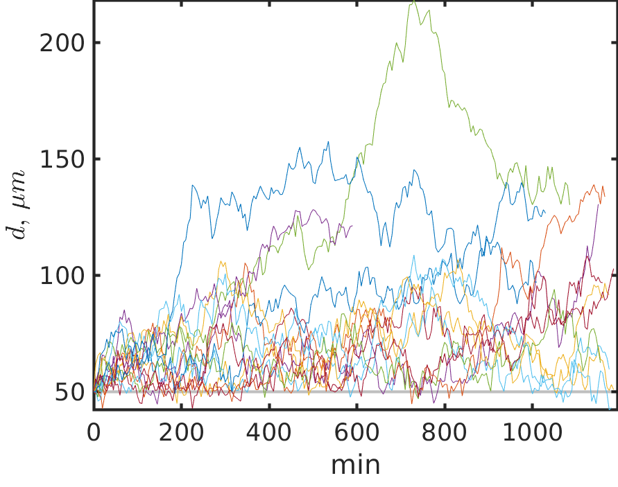
(a)

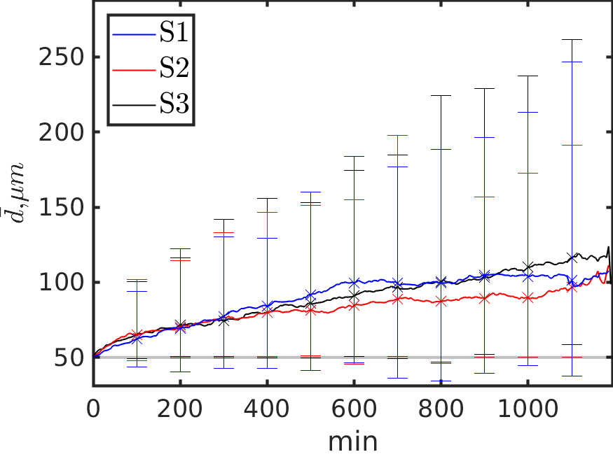
(b)

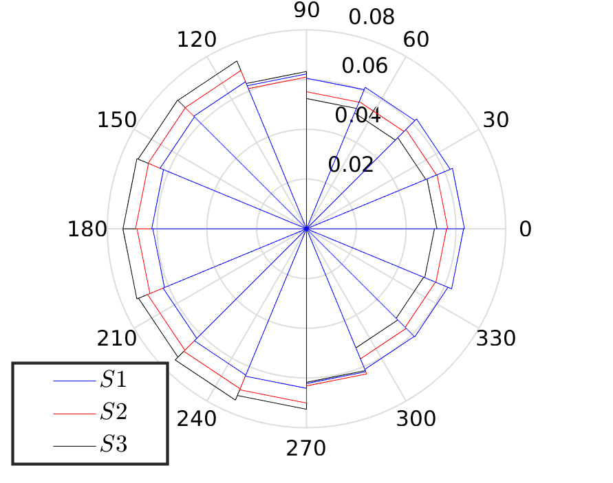
(c)

Figure 4: The opaque horizontal line indicates the distance of $2R_{cell}$, i.e. the cells in contact. (a) Cell centroid distance $d$ of 14 cell pairs corresponding to scenario S2. (b-c) Scenarios S1 in blue, S2 in red, S3 in black. (b) Ensemble averages $\bar{d}$ for each scenario. The corresponding error bars indicate ensemble minimum and maximum. (c) Relative frequency of binding events of cells with $\bar{C}^{i}=1$ and colliding at $0\degree$ for each scenario. Each sector corresponds to a single FA counting counterclockwise. Cell 2 is accounted for by reflection about south-north axis.

Since in our model the cells are not treated as hard spheres, it is possible that some overlaps may occur (Figure 4a,b). However, the slight overlap is followed by an increase in $d$ and separation (Figure 4a). Although the average distances $\bar{d}$ are similar (Figure 4b), increasing $\delta_{myo}$ and $\delta_{+}$ leads to a stronger response: the minimum of $d$ is consistently lower for S1 compared to S3 (Figure 4b) and FA formation away from the collision site is more frequent for S3 (Figure 4c). Notice that the cells need not obey the volume exclusion principle for eventual separation to occur and the stronger response in S3 implies that the separation can be modulated by modifying contractility and FA formation.

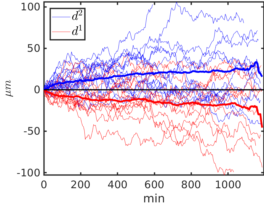
(a)

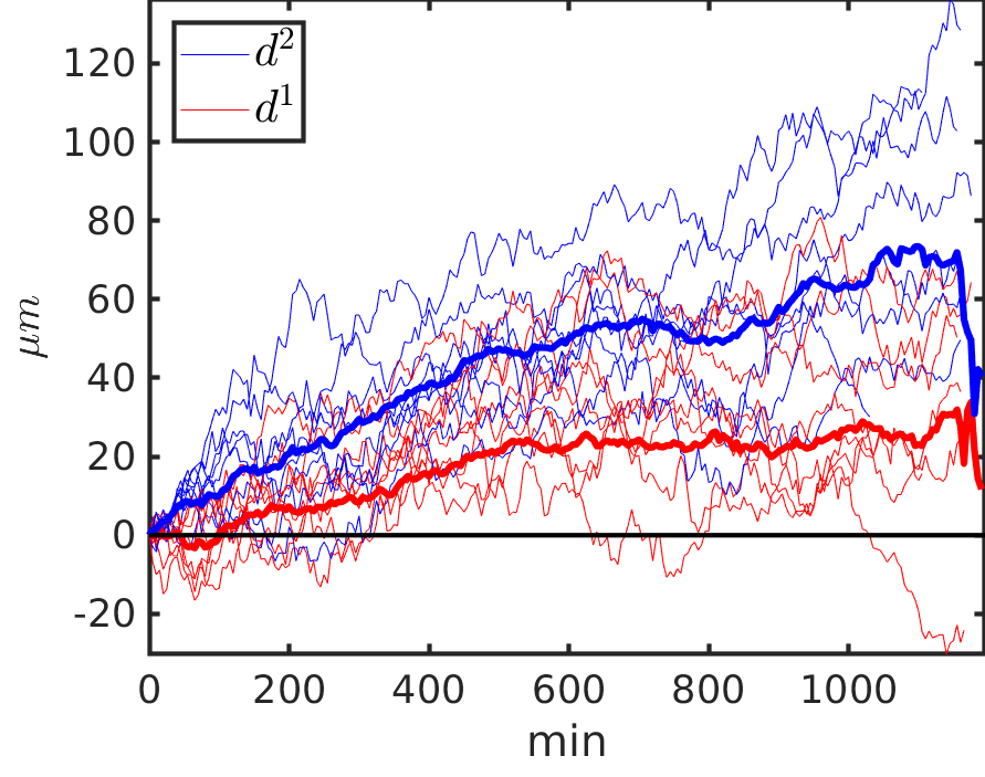
(b)

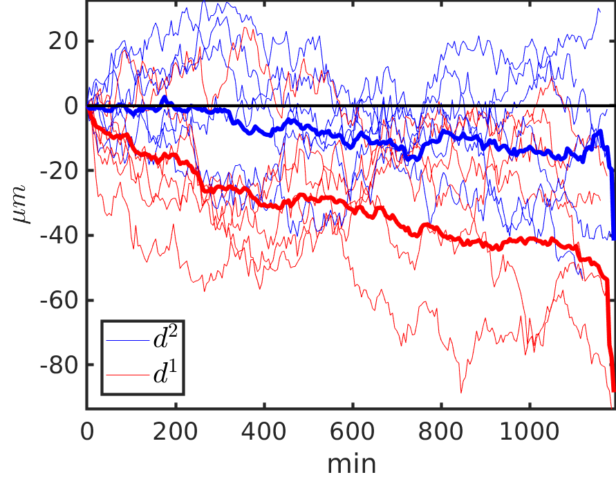
(c)

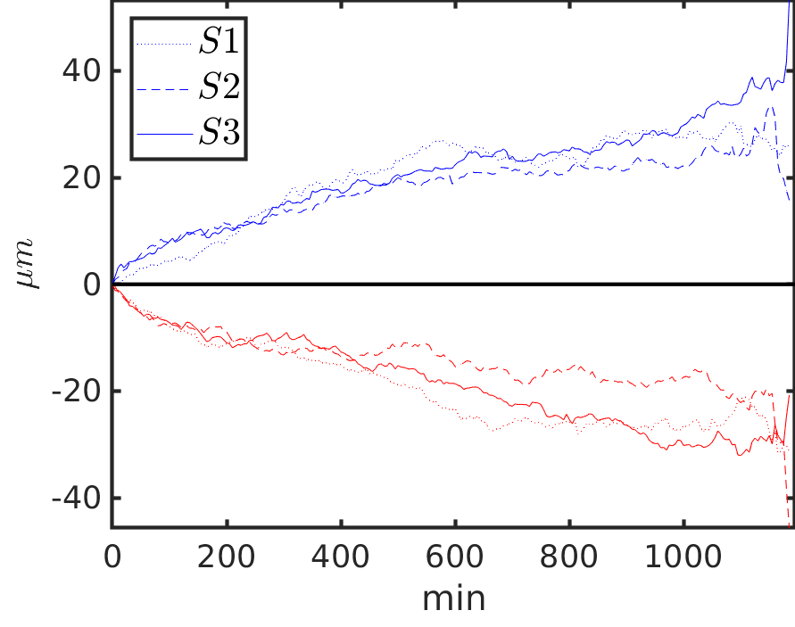
(d)

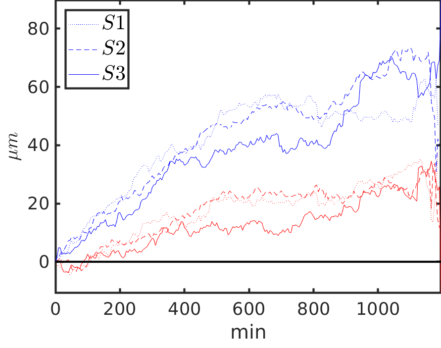
(e)

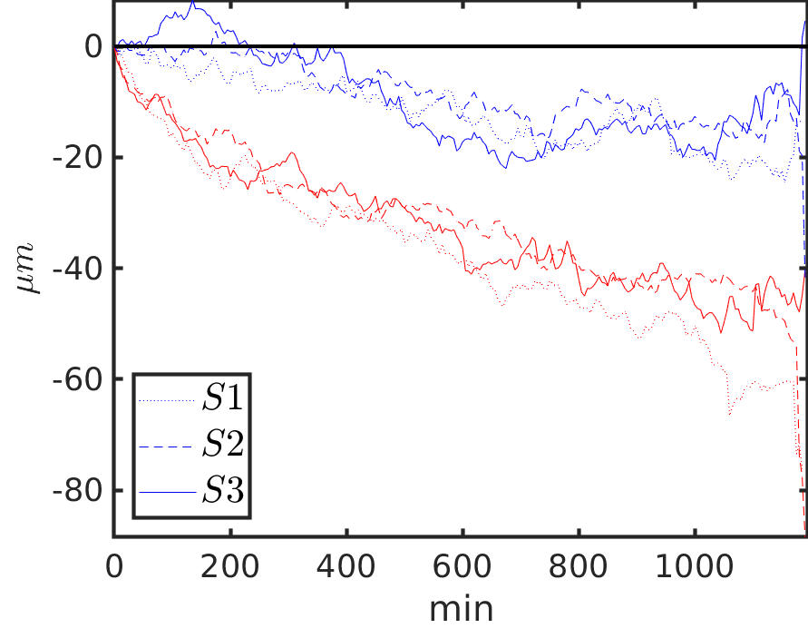
(f)

Figure 5: (a-c) The differences $d^{i}$ corresponding to scenario S2. Thick lines represent the corresponding ensemble averages. $d^{2}$ is colored in blue, $d^{1}$ in red. (a) A sample of 14 pairs. (b) and (c) The differences $d^{i}$, whose averages over time are positive and negative, respectively. Samples of 8 and 6 pairs are shown, respectively. (d-f) Ensemble averages of $d^{i}$ for scenarios S1 (dot), S2 (dash), and S3 (solid). Blue and red colored plots correspond to cells 1 and 2, respectively.(e) and (f) $d^{i}$ with positive and negative times averages.

Since increasing $d$ only suggests that the cells are separating, we examined their relative direction of motion after collision (Figure 5). Ensemble averages of $d^{i}$ in Figure 5d show that following collisions, the movement in the opposite directions is prevalent, which is in line with results in [7], [10]. It may also occur that cells follow one another after collision, as indicated by positive and negative time averages of $d^{1}$ and $d^{2}$ (Figure 5b,c). The ensemble averages in Figure 5(d-f) do not show a strong difference between the scenarios S1-S3. This suggests that varying the strength of cell response to collision does not have a significant effect on the relative direction of migration after the collision. In our simulations, $56\%$ of collided pairs moved in the opposite directions, compared to $\sim 65\%$ in [10].

Remark. Note that the collision times $t_{*}$ for each simulated pair are different. Thus, the number of cells at time $t$ after the collision time $t_{*}$ varies, and reduces towards the terminal time. This skews the values for ensemble averages and causes the abrupt changes in Figure 5.

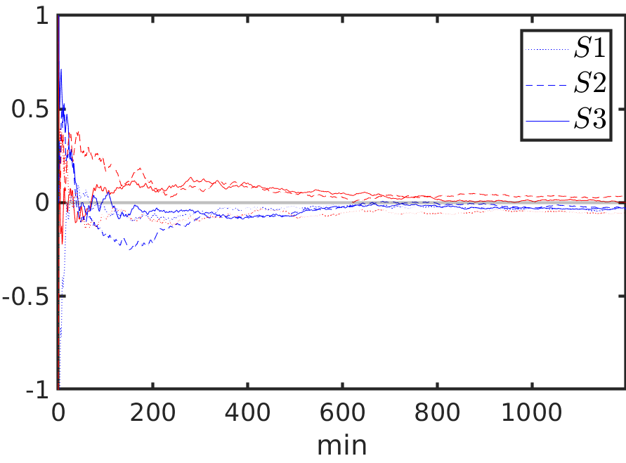
(a)

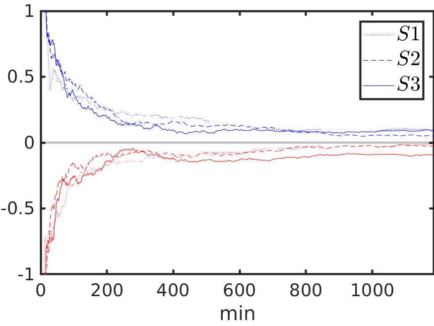
(b)

Figure 6: (a) and (b) Ensemble averages of normalized velocities before and after collisions, respectively, for scenarios S1 (dot), S2 (dash), and S3 (solid). Plots in red and blue correspond to cells 1 and 2, respectively. In (a) non-colliding pairs have also been accounted for.

Note that a freely migrating cell before collision is equally likely to move in either direction, as indicated by a rapid decay of normalized velocities to zero in Figure 6a. How fast does a cell become freely migrating after a collision? Figure 6b shows a much slower decay of the normalized velocities for the three scenarios. This suggests that either there are frequent follow up collisions after the first one, resulting in cell 1(2) moving left(right), or collisions lead to persistent movement in the opposite direction. It must be the latter, since in light of our results, cells separate (Figure 4b) and move away from each other (Figure 5d). Thus, in our model transient perturbations in cell motility lead to persistent, but decaying, alterations in migration dynamics. This is unexpected, since the collision state $\bar{C}^{i}$ of a cell is switched off after separation, i.e. the cell migrates freely. However, studies in [10] and [15] indicate that cells continue to move in opposite directions even after separation occurs.

4.1.2 Presence of a chemotactic gradient

We now explore how collision outcomes are affected in the presence of a chemotactic gradient, as experimental evidence in [10] suggest that CIL response is modulated by the strength of the external signal. As in [22], we suppose that $a^{+}_{j}\propto Q_{cue}$, i.e. the binding probability of the $j^{\text{th}}$ FA is proportional the (local) concentration of chemoattractant $Q_{cue}$ at the position of the FA.

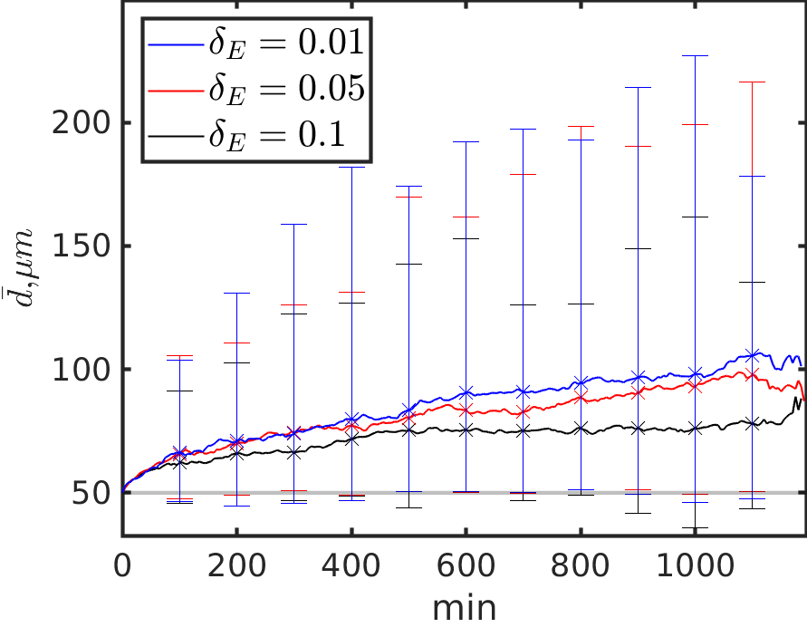
(a)

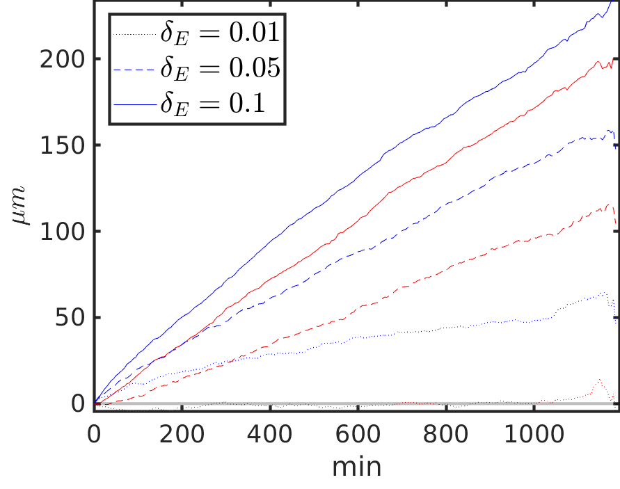
(b)

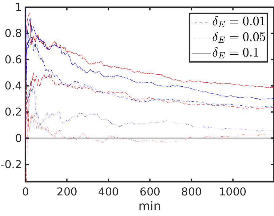
(c)

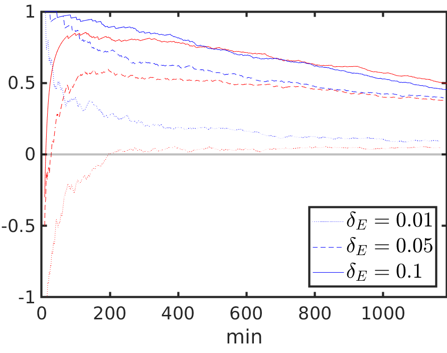
(d)

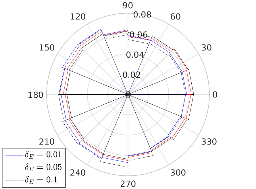
(e)

(f)

Figure 7: The effect of varying chemotactic signal strength $\delta_{E}$. (a,e,f) $\delta_{E}=0.01$ (blue), $0.05$ (red), $0.1$ (black). (a) Ensemble averages of cell-cell distances. (b,c,d) $\delta_{E}=0.01$ (dot), $0.05$ (dash), $0.1$ (solid). (b) Ensemble averages of $d_{1}$ (red) and $d_{2}$ (blue). (c) and (d) Ensemble averages of normalized velocities before and after collisions, respectively, of cells 1 (red) and 2 (blue). (e) and (f) Relative frequency of binding events after collision of cells 1 and 2. Dashed lines correspond to $\delta_{E}=0$.

We assume that $Q_{cue}$ has the following form:

$$Q_{cue}(\mathbf{x})=\begin{cases*}1+\delta_{E}x_{1},\text{ if $x_{1}>0$}\\ 1,\phantom{abcsasd}\text{else}\end{cases*},$$

where $\mathbf{x}$ is the position of an FA (in units of $R_{cell}$) in the lab reference frame, and $\delta_{E}>0$ indicates strength of the signal, i.e. there is a chemotactic gradient in the positive $x$-direction. We also take $\delta_{myo}=0.4$, $\delta_{+}=0.2$.

The influence of a chemotactic signal on CIL can be seen in Figure 7. We see that increasing the signal strength reduces average cell-cell separation (Figure 7a). Although the difference between the averages is slight (relative to cell size), the variance (as indicated by the error bars) of cell-cell distances is noticeably smaller for the case of the strongest signal. Moreover, after the collision, cells tend to move in the same direction following the signal, as shown in Figure 7b. This, together with what appears to be a plateauing of cell-cell distance (Figure 7a), suggests emergence of collective movement. Observe that reducing the signal strength leads to reduced propensity of cells to move in the same direction, in line with the results reported in [10]. Note that in [10] three scenarios with different EGF concentrations were explored. There, the gradients of EGF concentration were kept constant at $3.3nM$ per length of the lane. However, the relative changes in EGF concentrations were $\frac{5.5nM-2.2nM}{2.2nM}=1.6$, $\frac{9.9nM-6.6nM}{6.6nM}=0.5$, $\frac{14.1nM-10.8nM}{10.8nM}=0.3$ and reduced relative changes led to diminished alteration of a typical CIL response, which our simulations show as well.

Motion alignment is not immediate, as the amount of time during which cells move in the opposite directions after collision depends on the magnitude of the gradient (Figure 7d), compared to a rapid velocity alignment of uncollided pairs (Figure 7c).

We also see that the effect on adhesion dynamics of cells to the left and to the right of a collision point is different (Figure 7e,f). If the CIL signal in a cell and the chemotactic gradient are in the opposite directions, the affinity of FA association away from the contact reduces with increasing gradient strength (Figure 7e). However, if the signals are aligned, the FA binding dynamics does not appear to be significantly modified (Figure 7f). This suggests that in relation to adhesion dynamics, the chemotactic cue either reduces CIL response or has little to no effect. Interestingly, in [20] it was shown that elevated Rac1 activity (and hence enhanced adhesion to a substrate) away from the contact site (and in a free edge) is primarily due to cell-cell contacts, rather than to a chemoattractant.

4.2 Unconfined 2D setting

We now simulate our model in an unconfined 2D setting (see Appendix A for a general, non-binary system of cells) and investigate the effect of CIL on chemotaxing and non-chemotaxing cells. As was shown above, taking $\delta_{-}=0$ may lead to overlapping cells. Since in a general 2D setting a cell might have a contact with multiple cells at the same time (see Figure 8), it is possible (for arbitrary values of $\delta_{myo},\delta_{+}$, and $\delta_{-}$) that multiple cells overlap each other. Note that cells undergoing CIL do not crawl on top of each other. Thus, for cells undergoing CIL we take $\delta_{myo}=0.4,\delta_{+}=0.2,\delta_{-}=1$, and for cells not exhibiting it we take $\delta_{myo}=\delta_{+}=\delta_{-}=0$.

Figure 8: Schematic representation of CIL for non-binary collisions.

We also explore the interplay between CIL and chemotaxis in a heterogeneous population of cells. Namely, we investigate the effect of CIL on a mix of cells responsive and non-responsive to an external cue. For chemotaxing cells we take $\delta_{E}=0.05$.

In the following, we simulate 36 cells and evolve them for 20 hours, such that initially the cells are positioned as in Figure 9, and the distance between the centroids of neighboring cells is $2.4R_{cell}$.

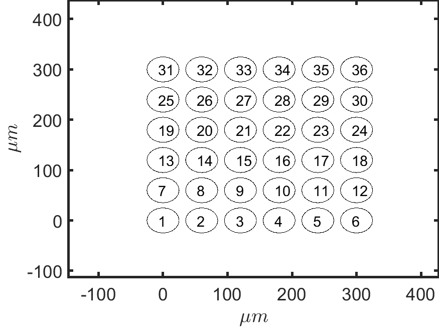
(a)

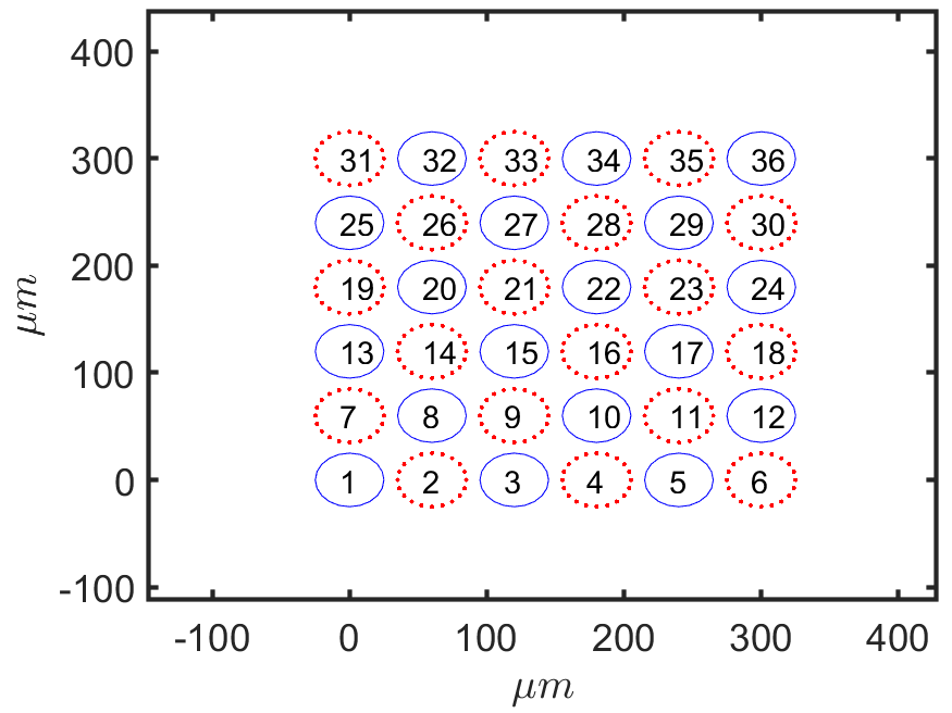
(b)

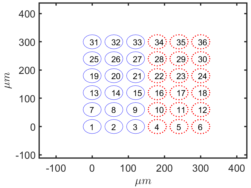
(c)

Figure 9: Initial configuration of cells. (a) Homogeneous population. (b,c) Heterogeneous populations of chemotaxing (blue, solid) and non-chemotaxing (red, dotted) cells.

4.2.1 Homogeneous population

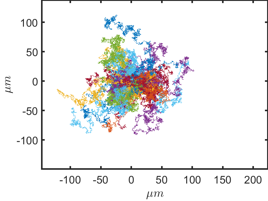
(a)

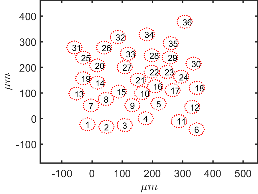
(b)

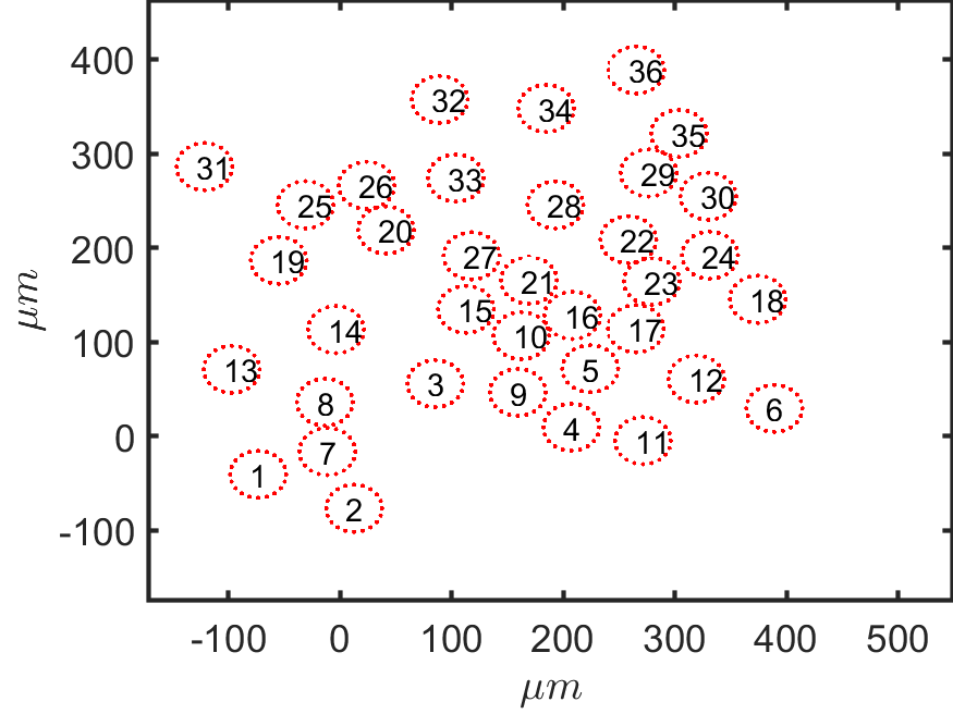
(c)

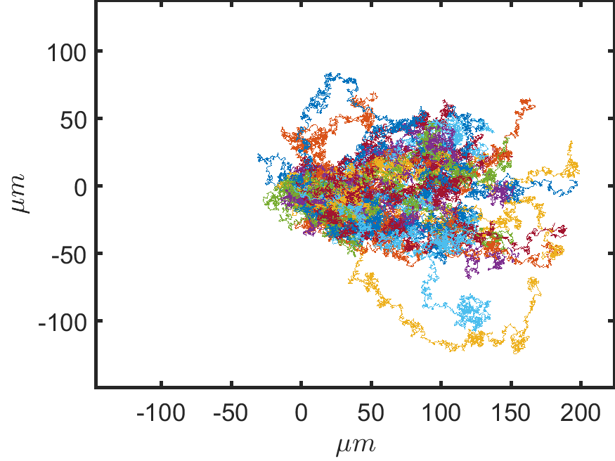
(d)

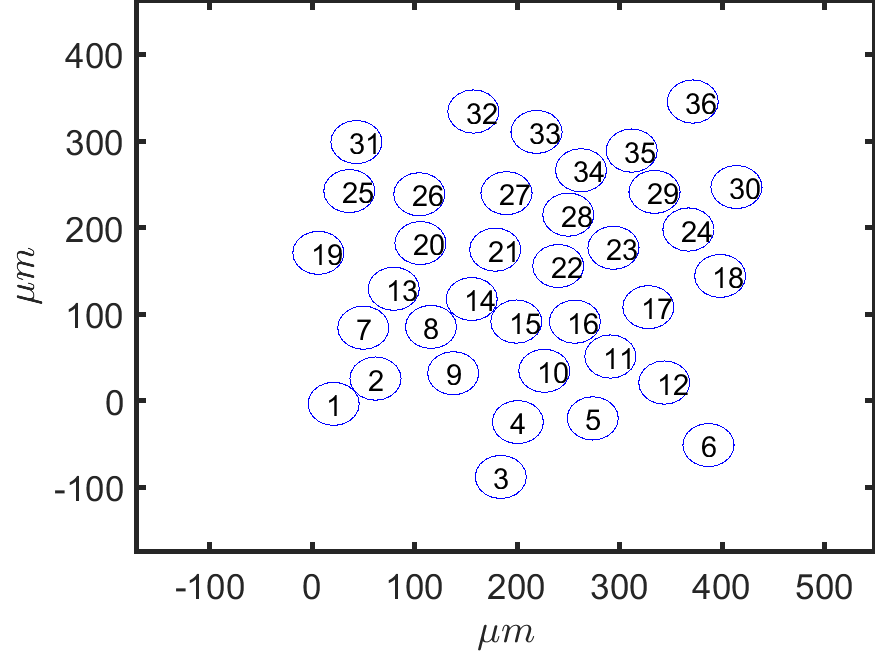
(e)

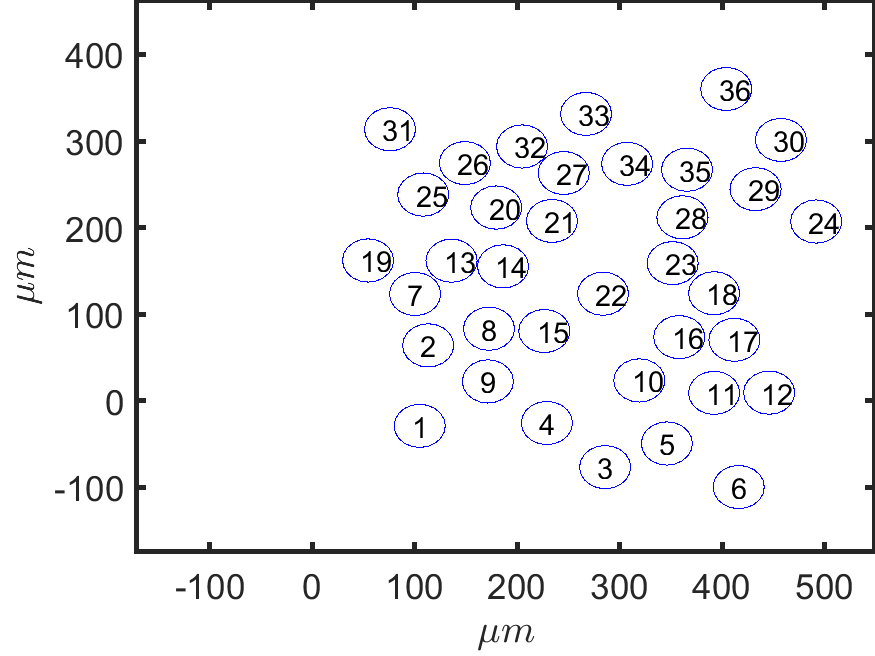
(f)

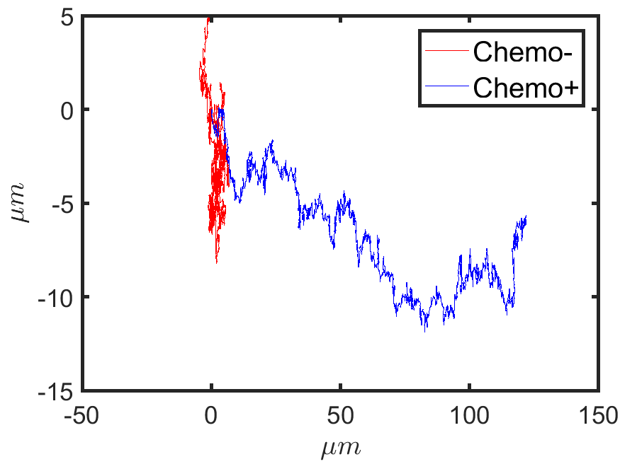
(g)

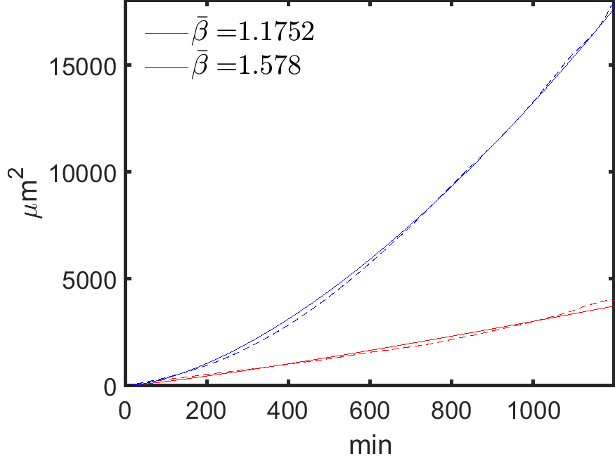
(h)

Figure 10: Simulation results for a homogeneous population of non-chemotaxing (top row) and chemotaxing cells (middle row). (a,d) Centered trajectories. (b,e) and (c,f) Cell positions at $t=600min,1200min$, respectively. (g) Centered trajectories of the cluster centers of mass. (h) Mean-squared displacement (dashed) of chemotaxing (blue) and non-chemotaxing (red) cells, and the fit $\widehat{msd}(t)$ (solid).

Simulation results for a homogeneous population of chemotaxing and non-chemotaxing cells are shown in Figure 10. We see that the biased migration of chemotaxing cells occurs in a cluster-like manner. In contrast, we see that the non-chemotaxing cells disperse randomly, such that the center of mass deviates very little as compared to cell dimensions ($R_{cell}=25\mu m$). Note that the motion of randomly migrating cells exhibits a superdiffusive character (Figure 10h), as indicated by fitting the mean-squared displacement to the curve $\widehat{msd}(t)=\beta_{0}t^{\bar{\beta}}$ (see Appendix in [22] for details). In [22], it was shown that non-interacting cells exhibit normal diffusive behavior ($\bar{\beta}\sim 1$) in the absence of any source of asymmetry affecting FA dynamics. Here, since the exponent $\bar{\beta}$ corresponding to non-chemotaxing cells is larger than one, we see that cell-cell collisions also lead to anomalous diffusion as $\bar{\beta}>1$. Comparing chemotaxing cells, we also see that $\bar{\beta}$ increases if cells collide with one another (in [22] $\bar{\beta}=1.34$ for the same value of $\delta_{E}$). Thus, we see that the average displacement increases due to CIL, despite the fact that motion ceases upon contact.

It has been hypothesized that superdiffusive motion is optimal for searching a target source, that itself diffuses [3], [8]. Thus, cancer cells that acquire ability to undergo homotypic CIL can find a diffusing source (e.g. VEGF) more efficiently and hence facilitate tumor progression. Interestingly, it has also been hypothesized that homotypic CIL facilitates dispersion of cancer cells [12], [17].

4.3 Inhomogeneous populations

We now explore the effects of heterotypic CIL between populations of chemotaxing and non-chemotaxing cells (Figure 9b,c). Here, cells always exhibit CIL when they collide with the members of the same group (see Appendix A.2.1).

When evenly mixed (Figure 9b), we see that heterotypic CIL does not have a significant impact on chemotaxing or non-chemotaxing cells (Figure 11), as the behavior of each subgroup resembles the case with the corresponding homogeneous populations. This suggests that in a disordered population of cells, homotypic, but not heterotypic CIL facilitates directed migration of cells (as $\bar{\beta}\approx 1.34$ in freely chemotaxing cells [22]). Nevertheless, notice that in this unclustered configuration, the chemotaxing cells are able to push their way out, leading to dispersion of the surrounding cells akin to billiard balls (Figure 11a,d): centered trajectories of the non-responsive cells show higher dispersion due to the repulsive interaction with the chemotaxing cells, who must push out the non-responsive cells to achieve the observed directed migration when such interaction is present. Clustering cells according to their responsiveness to an external cue, however, lead to a qualitatively different outcome. If responsive and non-responsive cells are separated as in Figure 9c, we see a cluster-like interaction when heterotypic CIL is present (Figure 12): the dividing line between the groups remains discernible for a long time (Figure 12b,c), which is not the case when the heterotypic CIL is absent (Figure 12e,f). This indicates that the initial clustering (Figure 9c) is conserved due to heterotypic interaction. Unlike the case of evenly mixed cells, we see that the dispersion of the non-chemotaxing cells is not as prominent (Figure 11a vs. Figure 12a), and the chemotaxing cells do not push out the non-responsive ones. In fact, we observe that the latter are being displaced in a sheet-like manner by the responsive cells. A similar behavior was observed in [21], although in that study the non-chemotaxing cells were themselves the source of a chemoattractant.

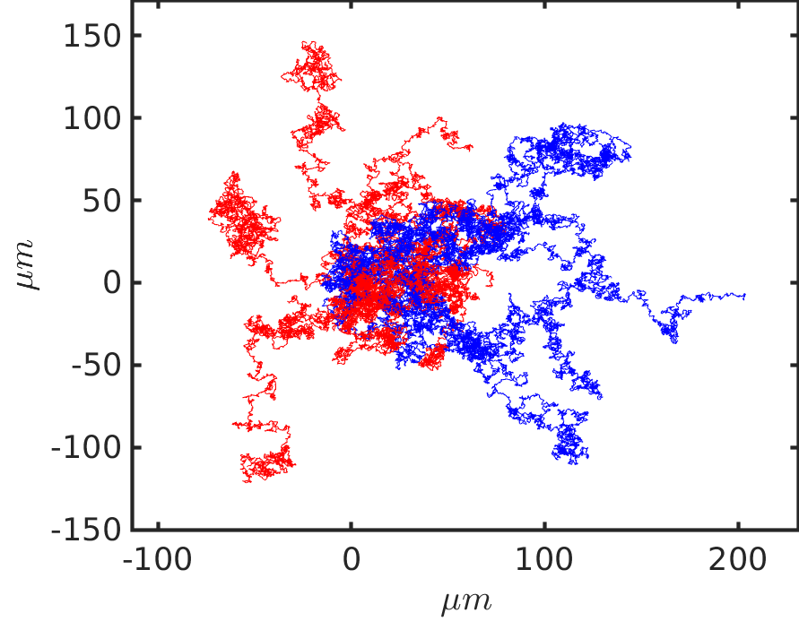
(a)

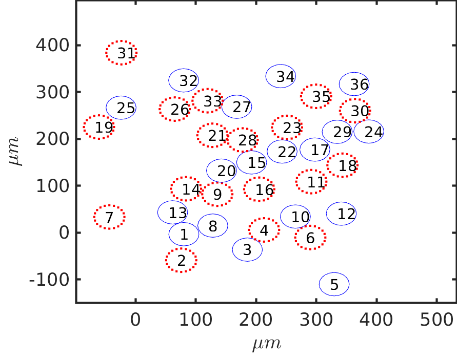
(b)

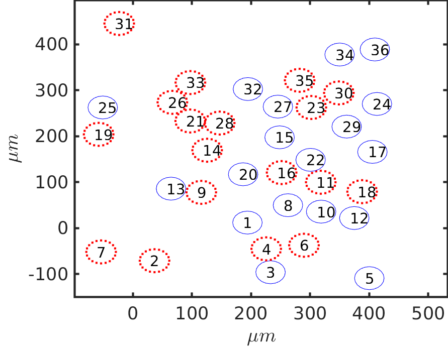
(c)

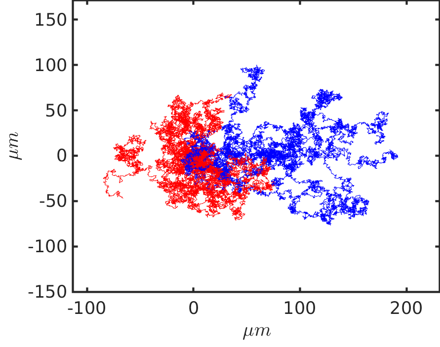
(d)

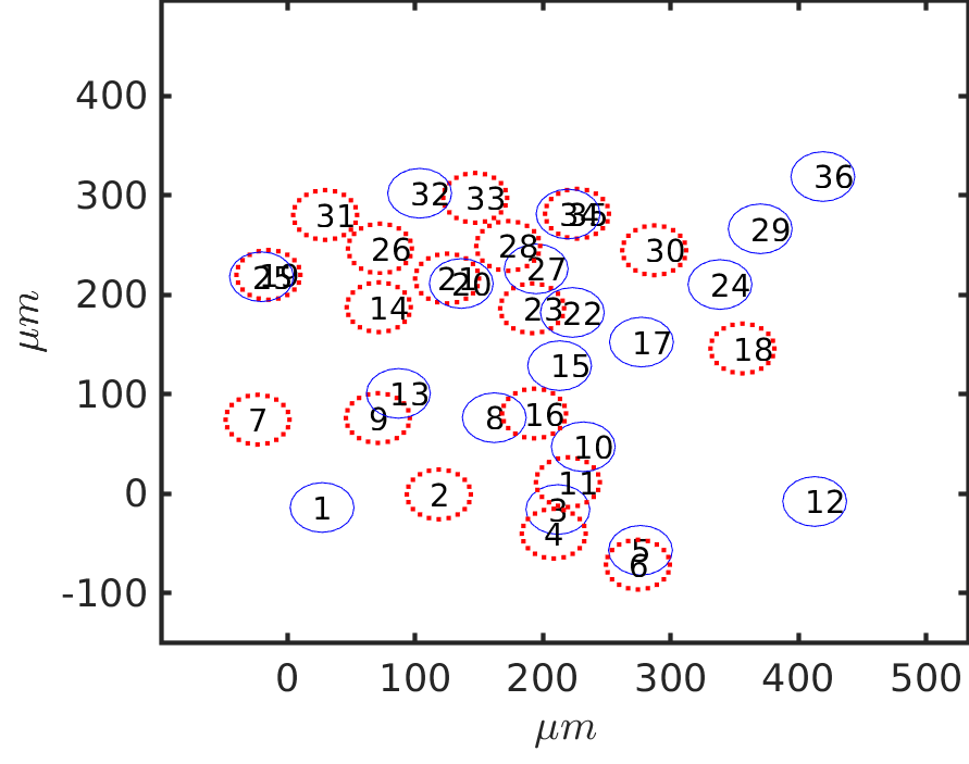
(e)

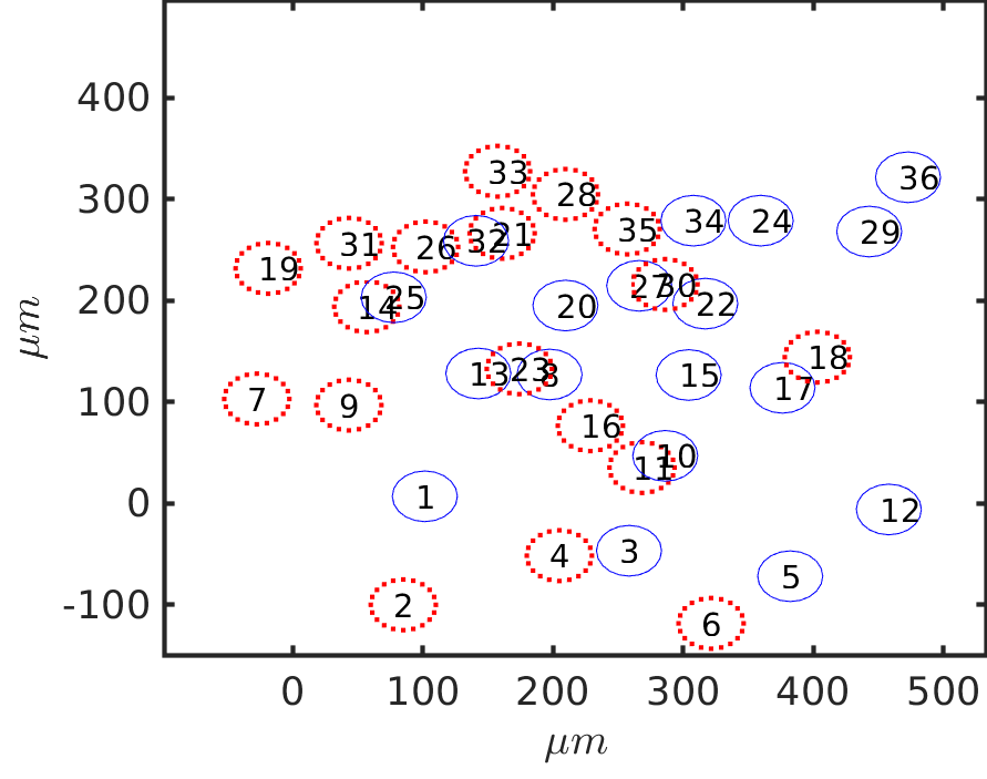
(f)

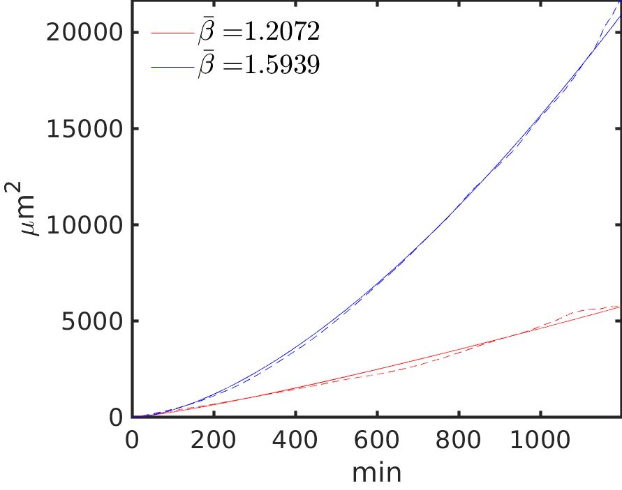
(g)

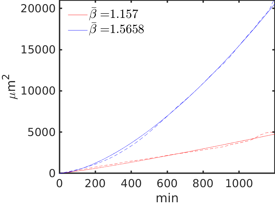
(h)

Figure 11: Simulation results for the mixed population with (top row) and without (middle row) heterogeneous CIL. Initially, cells are positioned as in Figure 9b. (a,d) Centered trajectories of 9 chemotaxing (blue) and non-chemotaxing (red) cells. (b,e) and (c,f) Positions of chemotaxing (blue, solid) and non-chemotaxing (red, dotted) cells at $t=600min$ in (b,e) and at $t=1200min$ in (c,f). (g,h) Mean squared displacements of chemotaxing (blue) and non-chemotaxing (red) cells with (g) and without heterotypic CIL (h).

Such displacement induces the non-chemotaxing cells to align their motion with the direction of an external cue (Figure 12g), although the effect of heterotypic CIL is slight. On the other hand, we see that directed migration of the chemotaxing cells is impeded (Figure 12h), which is also reflected in the reduced average displacement (Figure 12i). Altogether, these results suggest that the role of heterotypic CIL varies with the distribution of the cell population: it may either facilitate dispersion (Figure 11) or induce directed motion in otherwise randomly migrating cells (Figure 12). Its loss, however, is beneficial for tactic migration irrespective of spatial configuration.

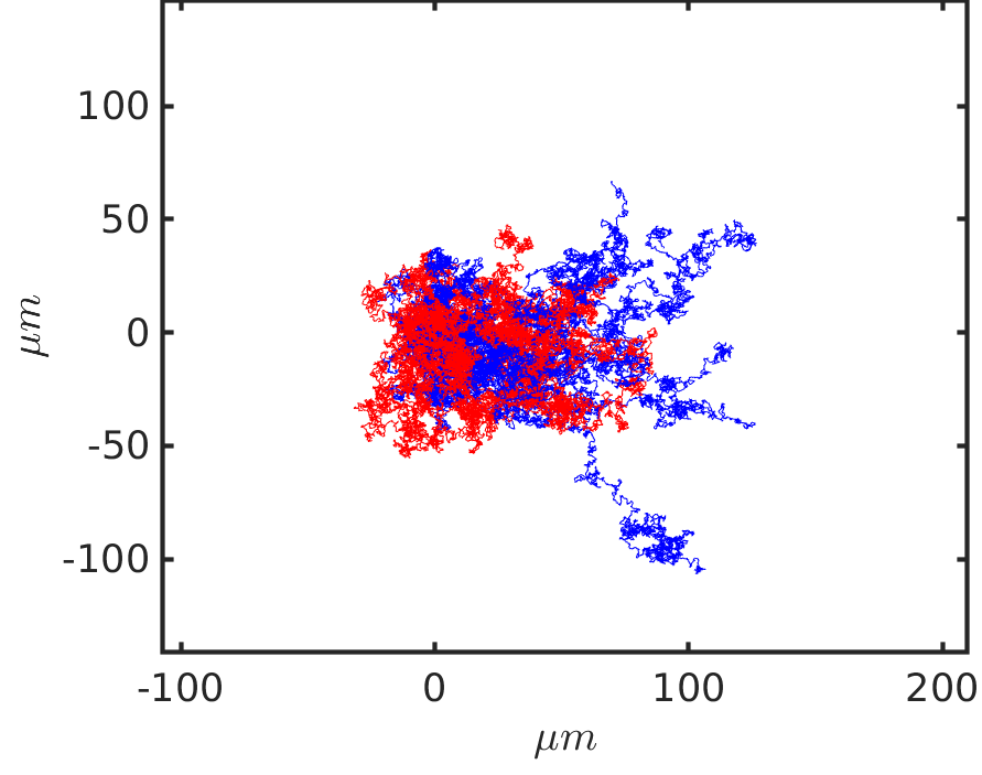
(a)

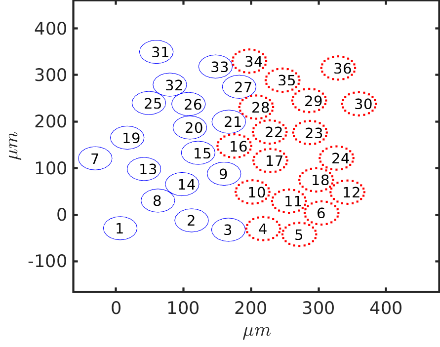
(b)

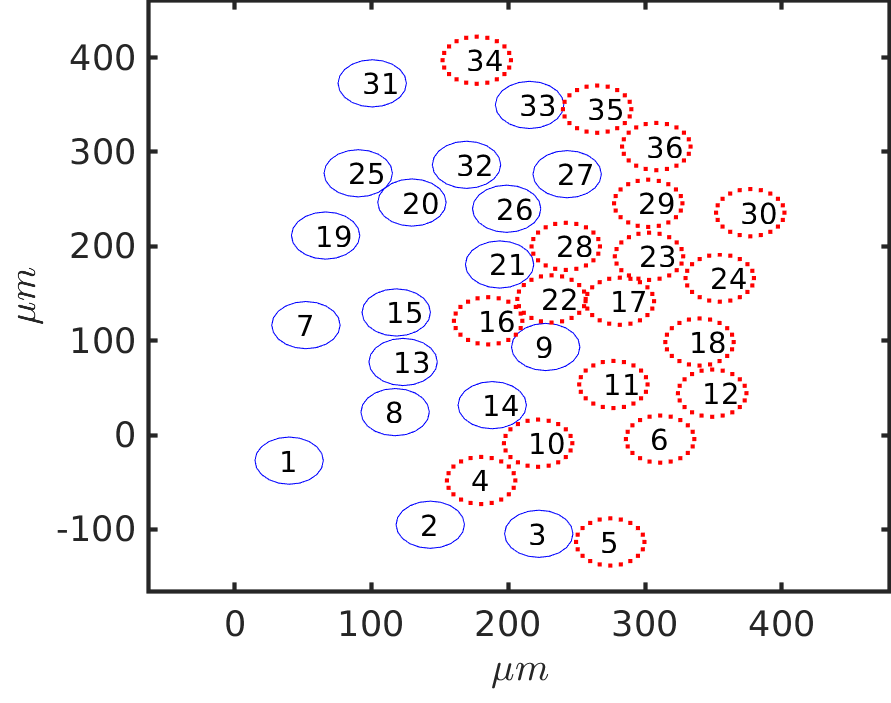
(c)

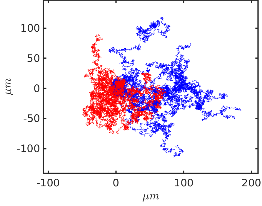
(d)

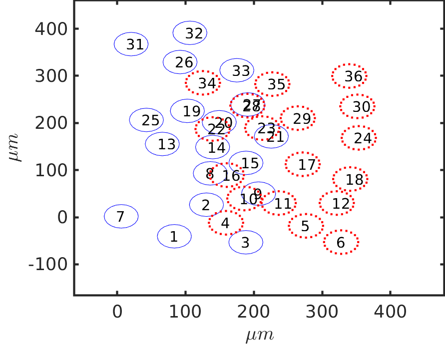
(e)

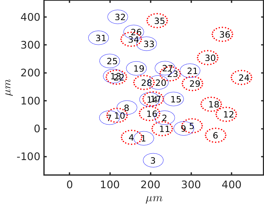
(f)

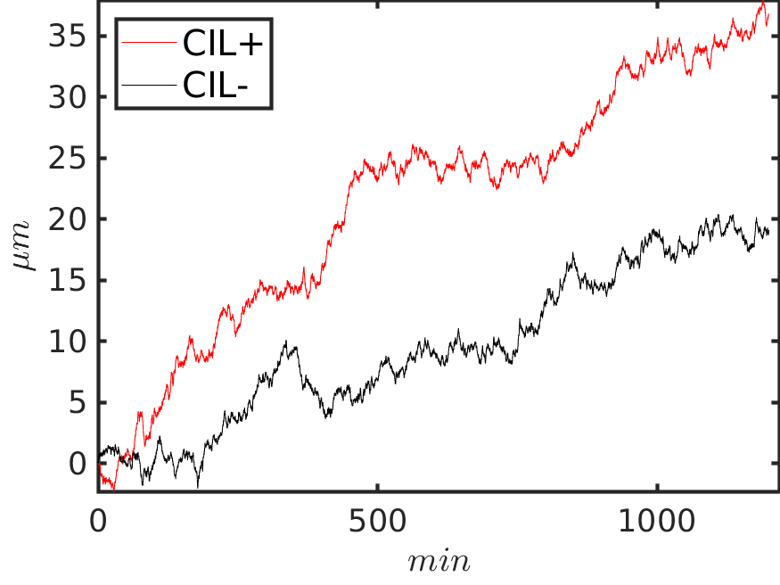
(g)

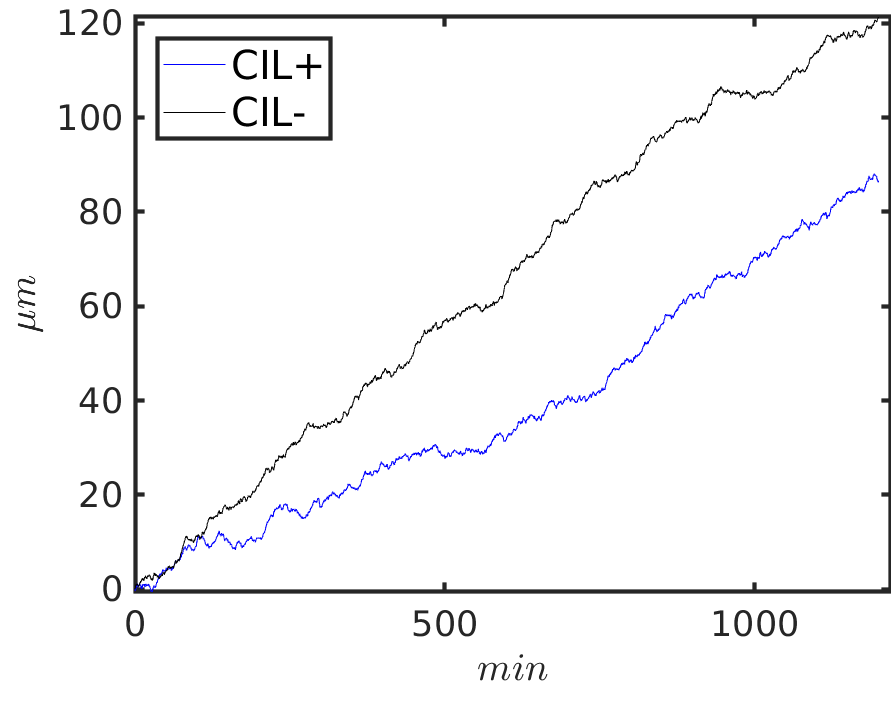
(h)

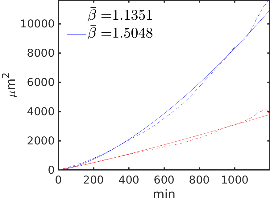
(i)

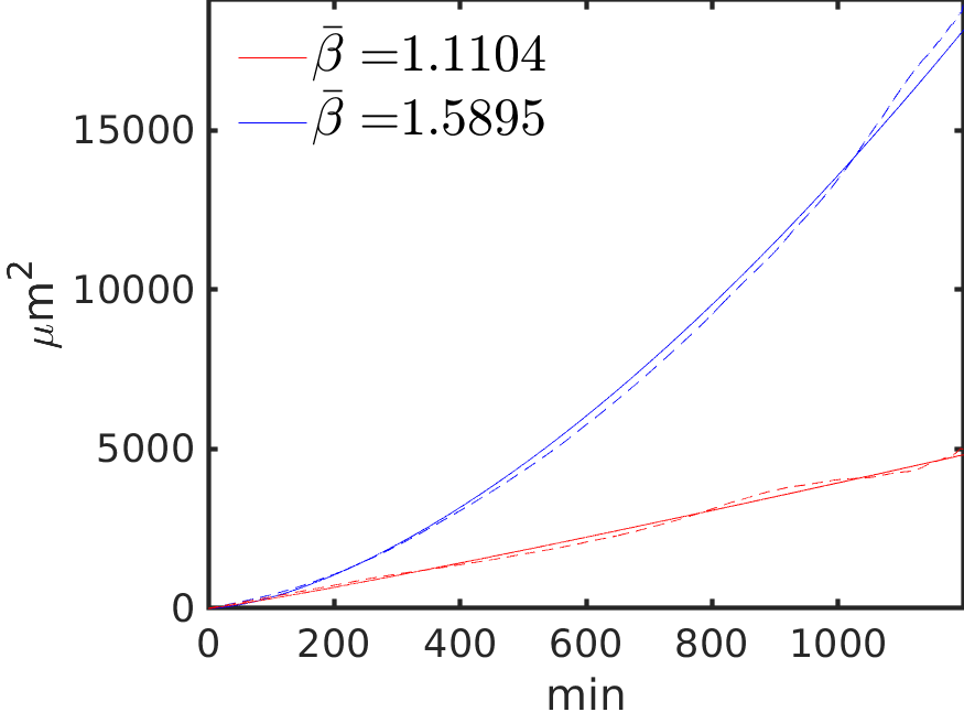
(j)

Figure 12: Simulation results for the separated population with (top row) and without (middle row) heterogeneous CIL. Initially, cells are position as in Figure 9c. (a,d) Centered trajectories of 9 chemotaxing (blue) and non-chemotaxing (red) cells. (b,e) and (c,f) Positions of chemotaxing (blue, solid) and non-chemotaxing (red, dotted) cells at $t=600min$ in (b,e) and at $t=1200min$ in (c,f). (g,h) $x$ components of non-chemotaxing (g) and chemotaxing (h) cells’ centers of mass with (colored) and without (black) heterotypic CIL. (i,j) Mean squared displacements of chemotaxing (blue) and non-chemotaxing (red) cells with (i) and without (j) heterotypic CIL.

5 Discussion and Outlook

In this paper we extended the single cell migration model from [22] to account for contact inhibition of locomotion arising as a result of cell-cell collisions. Here, the cells, exhibiting CIL response, alter cell-substrate adhesions dynamics and SF contractility following contact with another cell. Mathematically, the model is described by a piecewise deterministic process, whereby collisions occur when some deterministic components (cell-cell distances) reach a corresponding value, and cell motility itself emerges due to mechanochemically mediated stochastic adhesion dynamics. Consequently, the outcome of a collision is also determined stochastically, as reported in [7], [10], [15].

Mimicking the experimental setup in [10], we simulated binary collisions between cells migrating confined to a 1D lane. In this setting, we did not invoke the volume exclusion principle, and showed that a CIL response can be explained solely due to increased cell-substrate adhesion away from the collision site and increased actomyosin contractility in its vicinity. Although cell overlaps occur, we see that by strengthening the CIL response we can reduce its occurrence (Figure 4b). Our results also show that an external cue can modulate CIL response, in line with [10]. Specifically, typical CIL response can be overridden by chemotaxis (Figure 7) if post collision velocity is not aligned with the chemotactic gradient.

In an unconfined setting, we simulated the effects of homo- and heterotypic CIL. We found that homotypic CIL leads to increased cell displacement of chemotaxing and non-chemotaxing cells (Figure 10h). We also found that the spatial configuration of heterogeneous cells can have an impact on how heterotypic CIL affects migration of cells. In a disordered population it can facilitate the dispersion of randomly migrating cells (Figure 11), while letting directed migration to be unhindered. When separated into groups, our simulations suggest that directed movement can be induced in non-chemotaxing cells (Figure 12), as reported in [20]. Altogether, simulations in the unconfined setting suggest that homotypic, but not heterotypic CIL, is advantageous for dispersive and invasive migration of cells. It has been speculated that such CIL behavior is responsible for the initial spread of cancer cells [12], [17].

Guided by the study in [7], we assumed that CIL response between two cells is transient and independent of each other. That is, immediately following the collision, cell dynamics and FA event probabilities in both cells are decoupled. However, there is evidence that a mechanical coupling is established prior to repulsion [18]. Moreover, some cells exhibiting homotypic CIL tend to disperse and reaggregate into small clusters, which increases their chemotactic efficiency [20]. Thus, addressing mechanical coupling by including cell-cell adhesions represents one of the avenues for future work, whereby collective migration could be investigated further.

Appendix A General CIL model

In order to construct a motility model with $N$ colliding cells, we proceed as in [22]. In particular, we first provide a formal derivation of the survival function for the next event time and the distribution of the next event index for $N$ cells (the special case of which is given in (3.4)-(3.5)). Then we formulate our model as a piecewise deterministic Markov process (see [6] for a comprehensive treatment), similarly as in [22], but including collisions.

A.1 Preliminaries

Let $N$ be the number of cells and let $\mu^{i},\mathbf{Y}^{i}$, $i=1,\ldots,N$, be defined as in Section 3, and let $\bm{\mu}=(\mu^{1},\ldots,\mu^{N})$. Let $\mathbf{C}^{i}(t)\in\{0,1\}^{N}$ denote the collision state of cell $i$ at time $t$ with other cells:

$$C^{i}_{k}=\begin{cases*}1,\text{if cell $i$ is in collision state with cell $k$}\\ 0,\text{else},\end{cases*}$$

where $k=1,\ldots,N$ and we assume that $C^{i}_{i}=0$. Let $\mathbf{\Phi}^{i}(t)\in[0,2\pi)^{N}$ denote the vector of collision angles of cell $i$ with other cells, such that $\Phi^{i}_{i}(t)=0$. For $N=2$ in Section 3, for example, we have $\mathbf{C}^{1}(\mathcal{T}_{k})=(0,1)$ and $\mathbf{\Phi}^{2}(\mathcal{T}_{k})=(\pi,0)$. For ease of notation, let $\mathbf{X}^{i}=(\mathbf{x}^{i},\mathbf{x}^{i}_{n},\theta^{i},\mathbf{\Phi}^{i},\mathbf{d}^{i})$, where $\mathbf{d}^{i}$ is defined in (A.5), and $\mathbf{A}=(\mathbf{A}^{1},\ldots,\mathbf{A}^{N})$ for $\mathbf{A}\in\{\mathbf{Y},\mathbf{C},\mathbf{X}\}$.

Since there are $N$ cells and $2M$ possible reactions for each cell (binding and unbinding of an FA), then there are $2MN$ possible reactions among all cells. Let $a_{j^{\prime}}(\bar{\bm{\mu}},\mathbf{y},\mathbf{c},\mathbf{X}(t))dt$ be the probability, given $\mathbf{X}(t)$ and $\mathbf{A}(t)=\mathbf{a}$, for $\mathbf{A}\in\{\bm{\mu},\mathbf{Y},\mathbf{C}\}$ and $\mathbf{a}\in\{\bar{\bm{\mu}},\mathbf{y},\mathbf{c}\}$, that a reaction $j^{\prime}=1,\ldots,2MN$ will occur in the time interval $[t,t+dt)$.

Finally, let $K_{time}(\tau|t,\bar{\bm{\mu}},\mathbf{y},\mathbf{c},\mathbf{X}(t))d\tau$ be the probability that a reaction occurs in the time interval $[t+\tau,t+\tau+d\tau)$ and let $K_{index}(j^{\prime}|t,\tau,\bar{\bm{\mu}},\mathbf{y},\mathbf{c},\mathbf{X}(t))$ be the probability of reaction $j^{\prime}$, given that it occurs at time $t+\tau$. Then, we have [22]:

$$K_{time} (\tau|t,\bar{\bm{\mu}},\mathbf{y},\mathbf{c},\mathbf{X}(t))$$

$$=a^{N}_{0}(\bar{\bm{\mu}},\mathbf{y},\mathbf{c},\mathbf{X}(t+\tau))\exp\left(-\int_{t}^{t+\tau}a^{N}_{0}(\bar{\bm{\mu}},\mathbf{y},\mathbf{c},\mathbf{X}(t+\tau^{\prime}))\tau^{\prime}\right)$$ (A.1)

and

$$K_{index}(j^{\prime}|t,\tau,\bar{\bm{\mu}},\mathbf{y},\mathbf{c},\mathbf{X}(t))=\frac{a_{j^{\prime}}(\bar{\bm{\mu}},\mathbf{y},\mathbf{c},\mathbf{X}(t+\tau))}{a^{N}_{0}(\bar{\bm{\mu}},\mathbf{y},\mathbf{c},\mathbf{X}(t+\tau))},$$ (A.2)

where $a^{N}_{0}=\sum_{j^{\prime}=1}^{2MN}a_{j^{\prime}}$. Here, we adopt the following convention:

• A reaction $j^{\prime}$ occurs in cell $i$ if $i=\lfloor\frac{j^{\prime}-1}{2M}\rfloor+1$.

• A reaction $j^{\prime}$ corresponds to a binding reaction of $j^{\text{th}}$ FA if $2j-1=j^{\prime}modN$, and to unbinding reaction of $j^{\text{th}}$ FA if $2j=j^{\prime}modN$.

Thus, $a^{+,i}_{j}=a_{2j-1+2M(i-1)}$ and $a^{-,i}_{j}=a_{2j+2M(i-1)}$ correspond, respectively, to binding and unbinding probability rates of the $j^{\text{th}}$ FA of cell $i$. For an example utilizing the above, see the special case with $N=2$ in Section 3.

A.2 PDMP formulation

Let $A:=\{1,\ldots,2^{N+MN+N^{2}}\}$ and let $\bm{\alpha}:A\rightarrow\{0,1\}^{N}\times\{0,1\}^{MN}\times\{0,1\}^{N^{2}}$ be a bijection. This is a mapping such that $\bm{\alpha}(\nu)=(\bm{\mu},\mathbf{Y},\mathbf{C})$ corresponds to motility, FA, and collision states of $N$ cells.

Let $\nu\in A$ and $\bm{\alpha}(\nu)=(\bm{\mu},\mathbf{Y},\mathbf{C})$. Let $D^{i,k}_{\nu}\subset\mathbb{R}$, $D^{i}_{\nu}\subset\mathbb{R}^{N}$, $D_{\nu}\subset\mathbb{R}^{N^{2}}$ be defined as:

$$D^{i,k}_{\nu} :=\begin{cases*}(-\infty,1],\phantom{aaBb}\text{if $C^{i}_{k}=0$ and $i,k\in I$}\\ (-\infty,\infty),\phantom{aab}\text{else}\end{cases*},$$ (A.3)

$$D^{i}_{\nu} :=\prod_{k=1}^{N}D^{i,k}_{\nu},\phantom{D}D_{\nu}:=\prod_{i=1}^{N}D^{i}_{\nu},$$ (A.4)

where $I\subset\{1,\ldots,N\}$ is the index set of cells exhibiting CIL. Let $\mathbf{d}^{i}:[0,\infty)\rightarrow D^{i}_{\nu}$, $i=1,\ldots,N$ be defined as:

$$d^{i}_{k}(t):=\exp\left(2R_{cell}^{2}-\frac{1}{2}\lVert\mathbf{x}^{i}(t)-\mathbf{x}^{k}(t)\rVert^{2}\right),\phantom{a}k=1,\ldots,N,$$ (A.5)

and let $\mathbf{d}:=\left(\mathbf{d}^{1},\ldots,\mathbf{d}^{N}\right)\in D_{\nu}$. This particular form of $d^{i}_{k}$ is chosen since it satisfies the following requirements, which we impose on $d^{i}_{k}$:

• $d^{i}_{k}$ must be a measure of distance between cells $i$ and $k$, such that it attains a unique value when the cells are in contact (in our case the value is one), and such that a certain range of values correspond to the case when the cells overlap.

• $d^{i}_{k}$ must be bounded and continuously differentiable.

Depending on the form of $d^{i}_{k}$, $D^{i}_{k}$ must be modified accordingly.

Let $\mathbf{X}^{i}:=(\mathbf{x}^{i},\mathbf{x}^{i}_{n},\theta^{i},\mathbf{\Phi}^{i},\mathbf{d}^{i})\in\mathbb{R}^{2}\times\Omega_{cell}\times[0,2\pi)\times D^{i}_{\nu}\times[0,2\pi)^{N}:=E^{i}_{\nu}$. For convenience of notation, we define $\bm{\alpha}^{i}_{\mathbf{A}}(\nu):=\mathbf{A}^{i}$, where $\mathbf{A}\in\{\bm{\mu},\mathbf{Y},\mathbf{C}\}$. We also extend the definition of $u_{j}$ in (3.1):

$$u_{j}(\mathbf{X}^{i},\bm{\alpha}^{i}_{\mathbf{C}}(\nu)):=\begin{cases*}1,\phantom{abc}\Phi^{i}_{k}-\frac{\pi}{2}\leq\theta^{i}+(j-1)\frac{2\pi}{M}\leq\Phi^{i}_{k}+\frac{\pi}{2}\text{ and }C^{i}_{k}=1,\\ 0,\phantom{abc}\text{else},\end{cases*}$$

for some $k=1,\ldots,N$ and where $j=1,\ldots,M$. Then, we have:

$$T_{j} \rightarrow T_{j}(1+\delta_{myo}u_{j}(\mathbf{X}^{i},\bm{\alpha}^{i}_{\mathbf{C}}(\nu)))$$

$$\mathbf{F}_{j} \rightarrow\mathbf{F}_{j}(\mathbf{X}^{i},\bm{\alpha}^{i}_{\mathbf{C}}(\nu))$$

$$\mathbf{F} \rightarrow\mathbf{F}(\bm{\alpha}^{i}_{\mathbf{Y}}(\nu),\mathbf{X}^{i},\bm{\alpha}^{i}_{\mathbf{C}}(\nu)).$$

Let $E_{\nu}:=\prod_{i=1}^{N}E^{i}_{\nu}$ and define $\mathbf{H}^{i}_{\nu}:E_{\nu}\rightarrow\mathbb{R}^{5+2N}$ as:

$$\frac{d}{dt}\mathbf{X}^{i}=\begin{pmatrix}\bm{\alpha}^{i}_{\bm{\mu}}(\nu)\beta_{ECM}^{-1}\mathbf{F}(\bm{\alpha}^{i}_{\mathbf{Y}}(\nu),\mathbf{X}^{i},\bm{\alpha}^{i}_{\mathbf{C}}(\nu))\cdot\hat{\mathbf{r}}(\mathbf{x}^{i}_{n})\hat{\mathbf{r}}(\mathbf{x}^{i}_{n})\\ \beta_{cell}^{-1}\mathbf{F}(\bm{\alpha}^{i}_{\mathbf{Y}}(\nu),\mathbf{X}^{i},\bm{\alpha}^{i}_{\mathbf{C}}(\nu))\\ \bm{\alpha}^{i}_{\bm{\mu}}(\nu)\beta_{rot}^{-1}\lVert\mathbf{x}^{i}_{n}\rVert\mathbf{F}(\bm{\alpha}^{i}_{\mathbf{Y}}(\nu),\mathbf{X}^{i},\bm{\alpha}^{i}_{\mathbf{C}}(\nu))\cdot\hat{\bm{\varphi}}(\mathbf{x}_{n})\\ \mathbf{0}\\ -(\mathbf{x}^{i}-\mathbf{x}^{1})\cdot(\dot{\mathbf{x}}^{i}-\dot{\mathbf{x}}^{1})d^{i}_{1}\\ \vdots\\ -(\mathbf{x}^{i}-\mathbf{x}^{N})\cdot(\dot{\mathbf{x}}^{i}-\dot{\mathbf{x}}^{N})d^{i}_{N}\end{pmatrix}:=\mathbf{H}^{i}_{\nu}(\mathbf{X}).$$ (A.6)

This is simply an ODE system that governs the evolution of $\mathbf{X}^{i}$ between events. The equations governing $\mathbf{x}^{i},\mathbf{x}^{i}_{n}$, and $\theta^{i}$ were presented in Sections 2-3. Note that $\bm{\Phi}^{i}$ changes only when collisions occur, and is constant at all other times. For a collection of $N$ cells, we then have:

$$\frac{d}{dt}\mathbf{X}_{t} =\mathbf{H}_{\nu}(\mathbf{X}_{t})$$

$$\mathbf{X}_{0} =\mathbf{Z}\in E_{\nu}$$ (A.7)

where $\mathbf{H}_{\nu}:E_{\nu}\rightarrow\mathbb{R}^{5N+2N^{2}}$ and $\mathbf{H}_{\nu}:=(\mathbf{H}^{1}_{\nu},\ldots,\mathbf{H}^{N}_{\nu})$. One can also show that there exists a unique solution to (A.2), by using the result for a single cell model in [22].

Let $\phi_{\nu}:\mathbb{R}_{+}\times E_{\nu}\rightarrow E_{\nu}$ be the flow corresponding to (A.2). Note that a cell $i$ collides with a cell $k$, if $d^{i}_{k}\in\partial D_{\nu}^{i,k}=\{1\}$ for some $\nu\in A$ such that $C_{i}^{k}=0$. Thus, the boundary of $E_{\nu}$ plays an important role in addressing the collisions. Let $\partial E_{\nu}$ denote the boundary of $E_{\nu}$, and define $\partial^{*}E_{\nu}$, $\Gamma^{*}$ as:

$$\partial^{*}E_{\nu} :=\{\mathbf{X}\in\partial E_{\nu}:\phi_{\nu}(t,\mathbf{Z})=\mathbf{X},\phantom{a}(t,\mathbf{Z})\in\mathbb{R}_{+}\times E_{\nu}\}$$

$$\Gamma^{*} :=\{(\nu,\mathbf{X}):\nu\in A,\phantom{a}\mathbf{X}\in\partial^{*}E_{\nu}\}.$$

Let $E:=\{(\nu,\mathbf{X}):\nu\in A,\mathbf{X}\in E_{\nu}\}$ and define $t^{*}:E\rightarrow\mathbb{R}_{+}$ as:

$$t^{*}(\nu,\mathbf{X})=\inf\{t>0:\phi_{\nu}(t,\mathbf{X})\in\partial^{*}E_{\nu}\}.$$

Here, $t^{*}$ is simply the next collision time, given the state of the system $(\nu,\mathbf{X})\in E$. Let $a_{0}^{N}:E\rightarrow\mathbb{R}_{+}$ be defined as above:

$$a_{0}^{N}(\nu,\mathbf{X})=\sum_{j=1}^{2MN}a_{j}(\nu,\mathbf{X}),$$

where for ease of notation we write $a_{0}^{N}(\nu,\mathbf{X})=a_{0}^{N}(\bm{\alpha}(\nu),\mathbf{X})$ and $a_{j}(\nu,\mathbf{X})=a_{j}(\bm{\alpha}(\nu),\mathbf{X})$ for $(\nu,\mathbf{X})\in E$, $j=1,\ldots,NM$. We define

$$\mathcal{E}=\{B:B=\{(\nu,\mathbf{X}):\nu\in A,\phantom{a}\mathbf{X}\in\widetilde{E}_{\nu}\},\phantom{a}\widetilde{E}_{\nu}\in\mathbf{\mathcal{E}}_{\nu}\},$$

where $\mathbf{\mathcal{E}}_{\nu}$ denotes the Borel sets of $E_{\nu}$. Finally, let $(\Omega,\mathcal{F},\mathbb{P})$ be a probability space and define a transition measure $Q:\mathcal{E}\times E\cup\Gamma^{*}\rightarrow[0,1]$.

We now have all the ingredients to specify and construct a piecewise deterministic process of cell motility including collisions:

• Vector fields $\left(\mathbf{H}_{\nu},\nu\in A\right)$, given by (A.6), governing the system’s evolution between events and such that there exists a unique global solution to (A.2).

• An intensity function $a^{N}_{0}$, determining the arrival times of FA events, such that $s\mapsto a_{0}^{N}(\nu,\phi_{\nu}(s,\mathbf{X}))$ is integrable for $(\nu,\mathbf{X})\in E$.

• A transition measure $Q$ (to be specified below), determining the system’s state after an event, such that $(\nu,\mathbf{X})\mapsto Q(B,(\nu,\mathbf{X}))$ is measurable for fixed $B\in\mathcal{E}$, and $Q(\cdot,(\nu,\mathbf{X}))$ is a probability measure for $(\nu,\mathbf{X})\in E$.

Suppose the process $(\nu_{t},\mathbf{X}_{t})$ starts at $(\nu_{0},\mathbf{X}_{0})\in E$. Let the survival function $S$ be defined by

$$S(t)=\begin{cases*}\exp\left(-\int_{0}^{t}a^{N}_{0}(\nu_{0},\phi_{\nu_{0}}(s,\mathbf{X}_{0}))ds\right),\phantom{a}t<t^{*}(\nu_{0},\mathbf{X}_{0})\\ 0,\phantom{aaaaaaaaaaaaaasdasaaaaAaaa}t\geq t^{*}(\nu_{0},\mathbf{X}_{0}).\end{cases*}$$ (A.8)

Then, $\mathbb{P}(\mathcal{T}_{1}>t)=S(t)$, where $\mathcal{T}_{k}$ denotes the $k^{\text{th}}$ event time, and the motion of $(\nu_{t},\mathbf{X}_{t})$ is given by:

$$(\nu_{t},\mathbf{X}_{t})=\begin{cases*}(\nu_{0},\phi_{\nu_{0}}(t,\mathbf{X}_{0})),\phantom{a}t<T_{1}\\ (\nu_{1},\mathbf{X}_{1}),\phantom{aAAaaa}t=T_{1},\end{cases*}$$

where $(\nu_{1},\mathbf{X}_{1})$ is distributed according to $Q(\cdot,(\nu_{0},\phi_{\nu_{0}}(\mathcal{T}_{1},\mathbf{X}_{0})))$. At time $t=\mathcal{T}_{1}$, the next event time $\mathcal{T}_{2}$ is determined according to $\mathbb{P}(\mathcal{T}_{2}-\mathcal{T}_{1}>t)=S(t)$ and the motion continues as above. Note that after an event, the motion of $\mathbf{X}_{t}$ continues according to (A.2) until either an FA event (in one of the $N$ cells) or a collision occurs.

Let $(\nu,\mathbf{X})\in E\cup\Gamma^{*}$. Then, we have:

$$Q(\{\eta\}\times d\mathbf{X}^{\prime},(\nu,\mathbf{X}))=\mathbb{P}(\{\eta\}\times d\mathbf{X}^{\prime}\phantom{a}|\phantom{a}(\nu,\mathbf{X})\in\Gamma^{*})+\mathbb{P}(\{\eta\}\times d\mathbf{X}^{\prime}\phantom{a}|\phantom{a}(\nu,\mathbf{X})\notin\Gamma^{*}).$$

The first and the second terms on the right are, respectively, transition probabilities given that a collision or an FA event occurred. Using our previous results in [22], we have:

$$\mathbb{P}(\{\eta\}\times d\mathbf{X}^{\prime}\phantom{a}|\phantom{a}(\nu,\mathbf{X})\notin\Gamma^{*})$$

$$=\delta_{\mathbf{X}}(d\mathbf{X}^{\prime})\times\sum_{i=1}^{N}\left[\sum_{j=1}^{M}\delta_{\bm{\alpha}^{i}_{\bm{\mu}}(\eta),0}\frac{a^{+,i}_{j}(\nu,\mathbf{X})}{a^{N}_{0}(\nu,\mathbf{X})}\delta_{\bm{\alpha}^{i}_{\mathbf{Y}}(\eta)_{j},1}\prod_{j^{\prime}\neq j}^{M}\delta_{\bm{\alpha}^{i}_{\mathbf{Y}}(\eta)_{j^{\prime}},\bm{\alpha}^{i}_{\mathbf{Y}}(\nu)_{j^{\prime}}}\right.$$

$$\phantom{abAAAAAAAAAaa}\left.+\delta_{\bm{\alpha}^{i}_{\bm{\mu}}(\eta),1}\frac{a^{-,i}_{j}(\nu,\mathbf{X})}{a^{N}_{0}(\nu,\mathbf{X})}\delta_{\bm{\alpha}^{i}_{\mathbf{Y}}(\eta)_{j},0}\prod_{k\neq j}^{M}\delta_{\bm{\alpha}^{i}_{\mathbf{Y}}(\eta)_{k},\bm{\alpha}^{i}_{\mathbf{Y}}(\nu)_{k}}\vphantom{\sum_{j=1}^{M}}\right]$$

$$\phantom{abAAAAAAAa}\times\prod_{k\neq i}^{N}\delta_{\bm{\alpha_{\mu}}^{k}(\eta),\bm{\alpha_{\mu}}^{k}(\nu)}\prod_{j^{\prime}=1}^{M}\delta_{\bm{\alpha}^{k}_{\mathbf{Y}}(\eta)_{j^{\prime}},\bm{\alpha}^{k}_{\mathbf{Y}}(\nu)_{j^{\prime}}}\prod_{l=1}^{N}\delta_{\bm{\alpha_{C}}^{k}(\eta)_{l},\bm{\alpha_{C}}^{k}(\nu)_{l}}$$

$$\phantom{abAAAAAAAa}\times\prod_{k\neq i}^{N}\left[\delta_{\bm{\alpha_{C}}^{i}(\eta)_{k},1}\mathbf{1}_{\mathbb{R}^{+}\text{\textbackslash}\{0\}}(d^{i}_{k}-1)+\delta_{\bm{\alpha_{C}}^{i}(\eta)_{k},0}\mathbf{1}_{\mathbb{R}^{-}\cup\{0\}}(d^{i}_{k}-1)\right].$$

The first line indicates that components of $\mathbf{X}$ do not jump at an FA event time. The next two lines reflect the fact that an FA event changes the motility state and the state of one adhesion site. The fourth line corresponds to the fact that an FA event in a cell does not affect other cells. The last line indicates that the collision state of a cell is determined according to cell-cell distances at the time of an FA event.

Define the following for $(\nu,\mathbf{X})$:

$$B_{(\nu,\mathbf{X})} :=\{(m,l)\in\{1,\ldots,N\}^{2}:d^{m}_{l}=d^{l}_{m}=1,\bm{\alpha}^{m}_{\mathbf{C}}(\nu)_{l}=\bm{\alpha}^{l}_{\mathbf{C}}(\nu)_{m}=0\}$$

$$B^{c}_{(\nu,\mathbf{X})} :=\{1,\ldots,N\}^{2}\text{\textbackslash}B_{(\nu,\mathbf{X})},$$

i.e. tuples of cell indices that have collided, and the remaining pairs, respectively. Let $\mathbf{b}:\Gamma^{*}\rightarrow\mathbb{R}^{5N+2N^{2}}$ and $\hat{\bm{\Phi}}:E\rightarrow[0,2\pi)^{N}$ be given by:

$$b_{i}(\nu,\mathbf{X}) :=(\mathbf{x}^{i},\mathbf{x}_{n}^{i},\theta^{i},\hat{\bm{\Phi}}^{i}(\nu,\mathbf{X}),\mathbf{d}^{i})$$

$$\hat{\Phi}_{k}^{i}(\nu,\mathbf{X}) :=\begin{cases*}\Phi^{i}_{k},\phantom{AAAAa}\text{if $(i,k)\in B^{c}(\nu,\mathbf{X})$}\\ \hat{\varphi}(\mathbf{x}^{i},\mathbf{x}^{k}),\phantom{A}\text{else},\end{cases*}$$

where $\hat{\varphi}(\mathbf{x}^{i},\mathbf{x}^{k})$ is the polar angle at which a contact between cells $i$ and $k$ occurred. Then, we have:

$$\mathbb{P}(\{\eta\}\times d\mathbf{X}^{\prime}|(\nu,\mathbf{X})\in\Gamma^{*}) =\delta_{\mathbf{b}(\nu,\mathbf{X})}(d\mathbf{X}^{\prime})\prod_{(m,l)\in B(\nu,\mathbf{X})}\delta_{\bm{\alpha_{C}}^{m}(\eta)_{l},1}\delta_{\bm{\alpha_{\mu}}^{m}(\eta),0}$$

$$\phantom{a}\times\prod_{k=1}^{NM}\delta_{\bm{\alpha_{Y}}(\eta)_{l},\bm{\alpha_{Y}}(\nu)_{l}}\prod_{(m,l)\in B^{c}_{(\nu,\mathbf{X})}}\delta_{\bm{\alpha_{C}}^{m}(\eta)_{l},\bm{\alpha_{C}}^{m}(\nu)_{l}}\delta_{\bm{\alpha_{\mu}}^{m}(\eta),\bm{\alpha_{\mu}}^{m}(\nu)}.$$

The first line on the right reflects that at the time of collision, the contact angles, collision, and motility states jump to new values. The second line indicates that the FA, collision, and motility states of other cells are unaffected.

If the process hits the boundary (i.e. there is a collision), the post jump location is necessarily in $E$. That is, $\mathbb{P}(\{\eta\}\times d\mathbf{X}^{\prime}\phantom{a}|\phantom{a}(\nu,\mathbf{X})\in\Gamma^{*})=0$ if $\{\eta\}\times d\mathbf{X}^{\prime}\not\subset E$. This implies that expected number of events in a finite time is finite, and $\mathcal{T}_{k}\rightarrow\infty$ almost surely (see Chapter 2 in [6]).

A.2.1 Homotypic and heterotypic CIL

In order to take into account mixed populations with different CIL response, we only need to slightly modify the definition of $D^{i}_{k}$ in (A.3). Let $I_{1}\subset\{1,\ldots,N\}$, $I_{2}\subset\{1,\ldots,N\}$, be index sets of cells with and without CIL, respectively, such that $I_{1}\cap I_{2}=\emptyset$. Then:

$$D^{i,k}_{\nu} :=\begin{cases*}(-\infty,1],\phantom{aaBb}\text{if $C^{i}_{k}=0$, $i,k\in I_{1}$ or $i,k\in I_{2}$ }\\ (-\infty,\infty),\phantom{abA}\text{else},\end{cases*}$$

$$D^{i}_{\nu} :=\prod_{k=1}^{N}D^{i,k}_{\nu},\phantom{D}D_{\nu}:=\prod_{i=1}^{N}D^{i}_{\nu}.$$

Thus, only members of the same group undergo CIL. Here, in the absence of heterotypic CIL we effectively rule out collisions between members of different groups.

A.3 Simulation method

To simulate the constructed process we employ Algorithm 1 presented below.

1. Set $(\nu_{0},\mathbf{X}_{0})\in E$ and $t=\mathcal{T}_{0}=0$, $k=0$.

2. Generate interarrival time $\hat{\Delta}_{k}$ using Algorithm 2 in [22] applied to the ODE system (A.2) and the survival function (A.8).

3. Find $\mathbf{X}_{\mathcal{T}_{k}+\hat{\Delta}_{k}}=\phi_{\nu_{\mathcal{T}_{k}}}(\hat{{\Delta}}_{k},\mathbf{X}_{\mathcal{T}_{k}})$ and $\hat{B}_{\left(\nu_{\mathcal{T}_{k}},\mathbf{X}_{\mathcal{T}_{k}+\hat{\Delta}_{k}}\right)}$. Set $\Delta_{k}=\hat{\Delta}_{k}$.

4. If $\hat{B}_{\left(\nu_{\mathcal{T}_{k}},\mathbf{X}_{\mathcal{T}_{k}+\hat{\Delta}_{k}}\right)}\neq\emptyset$ (Collision)
   $\phantom{AB}\Delta_{k}=\min\left\{s>0:d^{m}_{l}(\mathcal{T}_{k}+s)=d^{l}_{m}(\mathcal{T}_{k}+s)=1,(m,l)\in\hat{B}_{\left(\nu_{\mathcal{T}_{k}},\mathbf{X}_{\mathcal{T}_{k}+\hat{\Delta}_{k}}\right)}\right\}$
   

5. Set $\mathcal{T}_{k+1}:=\mathcal{T}_{k}+\Delta_{k}$
   $\phantom{AB}(\nu_{\mathcal{T}_{k+1}},\mathbf{X}_{\mathcal{T}_{k+1}})\sim Q(\cdot,(\nu_{\mathcal{T}_{k}},\mathbf{X}_{\mathcal{T}_{k}+\Delta_{k}}))$
   $\phantom{AB}k:=k+1$

Algorithm 1 Simulation of the PDMP

Here, we use our previously developed method in [22] to simulate a general piecewise deterministic process. However, we now need to take into account collisions as well. To do so, we define

$$\hat{B}_{\left(\nu,\mathbf{X}\right)}:=\{(m,l)\in\{1,\ldots,N\}^{2}:d^{m}_{l}=d^{l}_{m}\geq 1,\phantom{a}\bm{\alpha}^{m}_{\mathbf{C}}(\nu)_{l}=\bm{\alpha}^{l}_{\mathbf{C}}(\nu)_{m}=0\}.$$ (A.9)

Note that if $(m,l)\notin\hat{B}_{\left(\nu_{t},\mathbf{X}_{t}\right)}$ and $(m,l)\in\hat{B}_{\left(\nu_{t},\mathbf{X}_{t+s}\right)}$, then this implies that a collision between cells $m$ and $l$ occurred in the time interval $[t,t+s]$.

After initialization in Step 1 of the algorithm below, we find the interarrival time $\hat{\Delta}_{k}$ of the next FA event in Step 2 using the method described in [22]. Then, in Step 3 we evolve the ODE system (A.2) and identify the cells, which collided in this time period. For each colliding pair, we find their collision time $s$, and their minimum in Step 4. The collision time $s\in(0,\hat{\Delta}_{k}]$ for $(m,l)\in\hat{B}_{\left(\nu_{\mathcal{T}_{k}},\mathbf{X}_{\mathcal{T}_{k}+\hat{\Delta}_{k}}\right)}$ is the root of

$$f(s)=f(\mathbf{X}_{\mathcal{T}_{k}+s})=d^{m}_{l}(\mathcal{T}_{k}+s)-1=0.$$ (A.10)

Note that after Step 3, the solution $\mathbf{X}_{t}$ of the ODE system (A.2) is available at the time points $t=\mathcal{T}_{k}+s_{i}$, where $i=0,\ldots,n$ and $s_{n}=\hat{\Delta}_{k}$. Thus,

$$f(s)=f(\mathbf{X}_{\mathcal{T}_{k}+s})=f(\phi_{\nu_{\mathcal{T}_{k}}}(s-s_{i},\mathbf{X}_{\mathcal{T}_{k}+s_{i}})).$$

Therefore, evaluation of (A.10) needed for a root finding method amounts to advancing the ODE system for a single time step of size $s-s_{i}$. This way, the amount of extra computations needed to find the collision time is minimized, which yields increasing computational savings as the number of cells $N$ increases. Finally, in Step 5 we set the time of the next event $\mathcal{T}_{k+1}$ and update the system according to the event occurred.

This method can be used to efficiently simulate an arbitrary PDMP, where solving an ODE system is expensive and the boundary hitting time is finite.

References

• [1] M. Abercrombie. The croonian lecture, 1978 - the crawling movement of metazoan cells. Proceedings of the Royal Society of London B: Biological Sciences, 207(1167):129–147, 1980.
• [2] M. Abercrombie and J. E. Heaysman. Observations on the social behaviour of cells in tissue culture: II. “monolayering” of fibroblasts. Experimental Cell Research, 6(2):293 – 306, 1954.
• [3] F. Bartumeus, J. Catalan, U. L. Fulco, M. L. Lyra, and G. M. Viswanathan. Optimizing the encounter rate in biological interactions: Lévy versus Brownian strategies. Phys. Rev. Lett., 88:097901, Feb 2002.
• [4] C. Carmona-Fontaine, H. K. Matthews, S. Kuriyama, M. Moreno, G. A. Dunn, M. Parsons, C. D. Stern, and R. Mayor. Contact inhibition of locomotion in vivo controls neural crest directional migration. Nature, 456(7224):957, 2008.
• [5] J. R. Davis, C.-Y. Huang, J. Zanet, S. Harrison, E. Rosten, S. Cox, D. Y. Soong, G. A. Dunn, and B. M. Stramer. Emergence of embryonic pattern through contact inhibition of locomotion. Development, 139(24):4555–4560, 2012.
• [6] M. H. A. Davis. Markov models and optimization. Chapman and Hall, 1993.
• [7] R. A. Desai, S. B. Gopal, S. Chen, and C. S. Chen. Contact inhibition of locomotion probabilities drive solitary versus collective cell migration. Journal of The Royal Society Interface, 10(88), 2013.
• [8] C. L. Faustino, L. R. da Silva, M. G. E. da Luz, E. P. Raposo, and G. M. Viswanathan. Search dynamics at the edge of extinction: Anomalous diffusion as a critical survival state. EPL (Europhysics Letters), 77(3):30002, 2007.
• [9] D. A. Kulawiak, B. A. Camley, and W.-J. Rappel. Modeling contact inhibition of locomotion of colliding cells migrating on micropatterned substrates. PLoS computational biology, 12(12):e1005239, 2016.
• [10] B. Lin, T. Yin, Y. I. Wu, T. Inoue, and A. Levchenko. Interplay between chemotaxis and contact inhibition of locomotion determines exploratory cell migration. Nature communications, 6:6619, 2015.
• [11] J. Löber, F. Ziebert, and I. S. Aranson. Collisions of deformable cells lead to collective migration. Scientific reports, 5:9172, 2015.
• [12] R. Mayor and C. Carmona-Fontaine. Keeping in touch with contact inhibition of locomotion. Trends in Cell Biology, 20(6):319 – 328, 2010.
• [13] B. Merchant, L. Edelstein-Keshet, and J. J. Feng. A Rho-GTPase based model explains spontaneous collective migration of neural crest cell clusters. Developmental Biology, 2018.
• [14] A. Roycroft and R. Mayor. Molecular basis of contact inhibition of locomotion. Cellular and Molecular Life Sciences, 73(6):1119–1130, 2016.
• [15] E. Scarpa, A. Roycroft, E. Theveneau, E. Terriac, M. Piel, and R. Mayor. A novel method to study contact inhibition of locomotion using micropatterned substrates. Biology Open, 2(9):901–906, 2013.
• [16] E. Scarpa, A. Szabó, A. Bibonne, E. Theveneau, M. Parsons, and R. Mayor. Cadherin switch during EMT in neural crest cells leads to contact inhibition of locomotion via repolarization of forces. Developmental Cell, 34(4):421 – 434, 2015.
• [17] B. Stramer and R. Mayor. Mechanisms and in vivo functions of contact inhibition of locomotion. Nature Reviews Molecular Cell Biology, 18(1), 2017.
• [18] B. Stramer, S. Moreira, T. Millard, I. Evans, C.-Y. Huang, O. Sabet, M. Milner, G. Dunn, P. Martin, and W. Wood. Clasp-mediated microtubule bundling regulates persistent motility and contact repulsion in drosophila macrophages in vivo. The Journal of Cell Biology, 189(4):681–689, 2010.
• [19] A. Szabó, M. Melchionda, G. Nastasi, M. L. Woods, S. Campo, R. Perris, and R. Mayor. In vivo confinement promotes collective migration of neural crest cells. The Journal of Cell Biology, 213(5):543–555, 2016.
• [20] E. Theveneau, L. Marchant, S. Kuriyama, M. Gull, B. Moepps, M. Parsons, and R. Mayor. Collective chemotaxis requires contact-dependent cell polarity. Developmental cell, 19(1):39–53, 2010.
• [21] E. Theveneau, B. Steventon, E. Scarpa, S. Garcia, X. Trepat, A. Streit, and R. Mayor. Chase-and-run between adjacent cell populations promotes directional collective migration. Nature cell biology, 15(7):763, 2013.
• [22] A. Uatay. A stochastic modeling framework for single cell migration: coupling contractility and focal adhesions. ArXiv e-prints, Oct. 2018.
• [23] M. L. Woods, C. Carmona-Fontaine, C. P. Barnes, I. D. Couzin, R. Mayor, and K. M. Page. Directional collective cell migration emerges as a property of cell interactions. PLoS ONE, 9(9):1–10, 09 2014.
• [24] J. Zimmermann, B. A. Camley, W.-J. Rappel, and H. Levine. Contact inhibition of locomotion determines cell–cell and cell–substrate forces in tissues. Proceedings of the National Academy of Sciences, 113(10):2660–2665, 2016.