Oscillatory Instabilities in Frictional Granular Matter

Abstract

Frictional granular matter is shown to be fundamentally different in its plastic responses to external strains from generic glasses and amorphous solids without friction. While regular glasses exhibit plastic instabilities due to a vanishing of a real eigenvalue of the Hessian matrix, frictional granular materials can exhibit a previously unnoticed additional mechanism for instabilities, i.e. the appearance of a pair of complex eigenvalues leading to oscillatory exponential growth of perturbations which are tamed by dynamical nonlinearities. This fundamental difference appears crucial for the understanding of plasticity and failure in frictional granular materials. The possible relevance to earthquake physics is discussed.

It is often stressed that the mechanical properties of frictional granular matter and of glassy amorphous solids share many similarities Liu and Nagel (1998); O’Hern et al. (2001); Wyart, M. (2005); Berthier and Biroli (2011); Ciamarra et al. (2011), although the effective forces in frictional solids are not derivable from a Hamiltonian. Here we show that the lack of a Hamiltonian description is responsible for previously unreported oscillatory instabilities in frictional granular matter. These oscillatory instabilities furnish a micromechanical mechanism for a giant amplification of small perturbations that can lead eventually to major events of mechanical failure. We will demonstrate this physics in the context of amorphous assemblies of frictional disks, but will make the point that the mechanism discussed here is generic for systems with friction. To motivate the new ideas recall that the understanding of plastic instabilities, shear banding and mechanical failure in athermal amorphous solids with an underlying Hamiltonian description had progressed significantly in the last twenty years. Beginning with the seminal papers of Malandro and Lacks Malandro and Lacks (1998, 1999) it became clear that an object that controls the mechanical responses of athermal glasses is the Hessian matrix. In an athermal (T=0) system of $N$ particles at positions $({\bm{r}}_{1},{\bm{r}}_{2}\cdots{\bm{r}}_{N})$ we define the Hamiltonian $U({\bm{r}}_{1},{\bm{r}}_{2},\cdots{\bm{r}}_{N})$. The Hessian matrix is

$$H^{\alpha\beta}_{ij}\equiv\frac{\partial^{2}U({\bm{r}}_{1},{\bm{r}}_{2},\cdots{\bm{r}}_{N})}{\partial r^{\alpha}_{i}\partial r^{\beta}_{j}}=-\frac{\partial F^{\alpha}_{i}}{\partial r^{\beta}_{j}}\ .$$ (1)

Here ${\bm{F}}_{i}$ is the total force on the $i$th particle, and in systems with binary interactions we can write ${\bm{F}}_{i}\equiv\sum_{j}{\bm{F}}_{ij}$ with the sum running on all the particles $j$ interacting with particle $i$. Being real and symmetric, the Hessian matrix has real eigenvalues which are all positive as long as the material is mechanically stable. Under strain, the system may display a saddle node bifurcation in which an eigenvalue goes to zero, accompanied by a localization of an eigenfunction, signalling a plastic instability that is accompanied by a drop in stress and energy Maloney and Lemaître (2004). Significant amount of work was dedicated to understanding the density of states of the Hessian matrix which differs in amorphous solids from the classical Debye density of purely elastic materials Wyart, M. (2005); Karmakar et al. (2010); Mizuno et al. (2017). The well known “Boson peak” was explained by the prevalence of “plastic modes” that can go unstable and do not exist in pure elastic systems. The system size dependence of the eigenvalues of the Hessian Karmakar et al. (2010), their role in determining the mechanical characteristics like the elastic moduli Hentschel et al. (2011), the failure of nonlinear elasticity in such materials Hentschel et al. (2011); Procaccia et al. (2016); Dailidonis et al. (2017), the relevance to shear banding and mechanical failure Dasgupta et al. (2012); Dasgupta et al. (2013a, b), all underline the importance of this approach to the theory of amorphous solids.

Alas, this useful approach appears to be irretrievably lost when we consider the available models for frictional granular media with both normal and tangential forces at every contact of two granules. The reason is two-fold. First, the tangential forces ${\bm{F}}_{ij}^{(t)}$ (see below for details), are not analytic because of the Coulomb constraint, $\left|{\bm{F}}_{ij}^{(t)}\right|\leq\mu\left|{\bm{F}}_{ij}^{(n)}\right|$, bounding the magnitude of the tangential force by the normal force ${\bm{F}}_{ij}^{(n)}$ multiplied by $\mu$ which is the friction coefficient. Secondly, and most importantly, model forces in frictional granular systems are not derivable from a Hamiltonian. In the most popular models, like the Hertz-Mindlin model Mindlin (1949), the inter-particle forces are derived by coarse graining the highly complex microscopic mechanics of compressed granules. As the resulting model forces cannot be derived from a Hamiltonian function, they are not energy conserving. We stress that this occurs also in the absence of viscous damping and before the Coulomb limit is reached.

To describe the failure of a granular systems as a dynamical instability we follow a two step approach. The first (maybe trivial looking) step that we propose here is to smooth out the approach to the Coulomb limit to allow differentiating the tangential force, and see Eq. (7) below. In the second step we consider frictional disks for which the coordinates now include the positions ${\bm{r}}_{i}$ of the centers of mass and the angles $\theta_{i}$ of each disk. The Newton equations of motion are written as

$$m_{i}\frac{d^{2}{\bm{q}}_{i}}{dt^{2}}={{\bm{F}}}_{i}({\bm{q}}_{1},{\bm{q}}_{2},\cdots,{\bm{q}}_{N})$$ (2)

where ${\bm{q}}_{i}\equiv\{{\bm{r}}_{i},\theta_{i}\}\equiv\{r_{i}^{x},r_{i}^{y},\theta_{i}\}$ and $m_{i}$ are masses or moments of inertia as is appropriate. It is important to stress that the forces in Eq. (2) depend only on the generalized coordinates ${\bm{q}}_{j}$, i.e. first derivatives do not appear. The stability of equilibria of Eq. (2) is then determined by an operator obtained from the derivatives of the force ${\bm{F}}_{i}$ on each particle with respect to the coordinates. In other words

$${\bm{J}}_{ij}\equiv-\frac{\partial{\bm{F}}_{i}}{\partial{\bm{q}}_{j}}.$$ (3)

The analogy between the operator ${\bm{J}}$ and the Hessian matrix is apparent. But there is a huge difference whose consequences are explored below. ${\bm{J}}$ is not a symmetric operator. Accordingly, it can have real eigenvalues as the Hessian, but it can also display a number of eigenvalues as complex conjugate pairs. When a pair complex eigenvalues, $\lambda_{1,2}=\lambda_{r}\pm i\lambda_{i}$, gets born, a novel instability mechanism develops. Indeed, these eigenvalues correspond to FOUR solutions $e^{i\omega t}$ to the linearized equation of motion with

$$i\omega_{1,2}=\omega_{i}\pm i\omega_{r}\ ,\quad i\omega_{3,4}=-\omega_{i}\pm i\omega_{r}\ .,$$ (4)

with $\omega_{r}\pm i\omega_{i}=\sqrt{\lambda_{r}\pm i\lambda_{i}}$. The first pair in (4) will induce an oscillatory motion with an exponential growth of any deviation ${\bm{q}}(0)$ from a state of mechanical equilibrium,

$${\bm{q}}(t)={\bm{q}}(0)e^{\omega_{i}t}\sin(\omega_{r}t).$$ (5)

The second pair represents an exponentially decaying oscillatory solution. We stress that this bifurcation is not a regular Hopf bifurcation. It needs at least four degrees of freedom (four first order or two second order differential equations). This is a somewhat unusual bifurcation that is appearing here due to the symmetry of Eqs. (2) that is a consequence of the absence of first derivatives. We also comment again that such a bifurcation is impossible in frictionless amorphous solids with a microscopic Hamiltonian.

To validate this theoretical scenario and explore its consequences we focus on a binary assembly of $N$ frictional disks of mass $m$ in a box of size $L^{2}$, half of which with radius $\sigma_{1}=0.5$ and the other half with $\sigma_{2}=0.7$. Under external stress they interact with binary interactions; the normal force is determined by the overlap $\delta_{ij}\equiv\sigma_{i}+\sigma_{j}-r_{ij}$ where ${\bm{r}}_{ij}\equiv{\bm{r}}_{i}-{\bm{r}}_{j}$. The normal force is Hertzian,

$${\bm{F}}_{ij}^{(n)}=k_{n}\delta_{ij}^{3/2}\hat{r}_{ij}\ ,\quad\hat{r}_{ij}\equiv{\bm{r}}_{ij}/r_{ij}\ .$$ (6)

The tangential force is determined by the tangential displacement ${\bm{t}}_{ij}$, the integral of the velocity at the contact point over the duration of the contact, rotated so as to enforce ${\bm{t}}_{ij}\cdot\hat{r}_{ij}=0$ at all times. This is quite standard Silbert et al. (2001). We deviate from the standard in the definition of the tangential force, that we assume to be

$${\bm{F}}_{ij}^{(t)}=-k_{t}\delta_{ij}^{1/2}\left[1+\frac{t_{ij}}{t^{*}_{ij}}-\left(\frac{t_{ij}}{t^{*}_{ij}}\right)^{2}\right]t_{ij}\hat{t}_{ij}\ ,$$

$$t^{*}_{ij}\equiv\mu\frac{k_{n}}{k_{t}}\delta_{ij}$$ (7)

with $k_{t}=2k_{n}/7$ Silbert et al. (2001). The derivative of the force with respect to $t_{ij}$ vanishes smoothly at $t_{ij}=t^{*}_{ij}$, and the Coulomb law is fulfilled. In the following, we use as units of mass, length and time $m$, $2\sigma_{1}$ and $\sqrt{m(2\sigma_{1})^{-1/2}k_{n}^{-1}}$, respectively. We also fix the friction coefficient to a high value, $\mu=10$, to emphasise that the existence of a Coulomb threshold is no responsible for the reported phenomenology, but we stress here that we have found analogous results for values of $\mu<1$.

We demonstrate the new type of instability considering a system with $N=500$. We prepare a mechanically equilibrated amorphous system with packing fraction 0.93 in a periodic 2-dimensional box. Upon straining we can choose to run two types of algorithms. The first is denoted Newtonian and is simply a solution of the Newton equations of motion with the given forces Eqs. (6) and (7) without damping. The second algorithm is called “overdamped” and is solving the same equations of motion but with a damping force that is proportional to the velocities of the disks with a coefficient of proportionality $\eta_{v}=m\eta_{0}$. We fix $\eta_{0}=10$. The damping timescale $\eta_{v}^{-1}$ is thus of the order of the time that sounds needs to travel one particle diameter Zhang and Makse (2005), making this dynamics overdamped. With damping, even in the presence of complex eigenvalues the oscillatory instability is suppressed by the damped dynamics. The numerical solution of the equation of motion is carried out with LAMMPS Plimpton (1995).

An athermal quasi static (AQS) shear protocol is now devised as follows: starting from the initial stable configuration the system is sheared along the horizontal direction ($x$) by the amount $\delta\gamma$, varied in the range $10^{-4}$ to $10^{-8}$ depending on the precision needed for the identification of the instability. Thus, each particle experiences an affine shift along $x$ depending on their vertical coordinates $r^{y}_{i}$, i.e. $\delta r_{i}^{x}=\delta\gamma r^{y}_{i}$. Next we run the overdamped dynamics to bring the system back to mechanical equilibrium where the net force on each particle is less than $10^{-8}$. After every such step we diagonalize the matrix ${\bm{J}}$ to find its eigenvalues. At some value of $\gamma$ we find for the first time the birth of conjugate pair of complex eigenvalues as seen in Fig. 1.

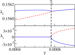
Figure 1: Upon increasing the strain $\gamma$ two modes with real eigenvalues $\lambda$ coalesce at $\gamma_{c}$ (dashed vertical lines), and a pair of complex conjugate modes gets born. The upper and the lower panels show the evolution of the real and of the imaginary components of these modes.

If we continue to increase the strain using the same protocol, we see the emergence of other complex pairs at the expense of real eigenvalues.

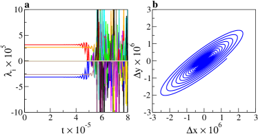
Figure 2: a: Time dependence of the imaginary component of all 1500 eigenvalues of the system, during a Newtonian simulation. b: typical spiral trajectory of a particle in the linear response regime.

In real granular systems, the dynamics is not overdamped. To explore how the system responds to the bifurcation we therefore run the Newtonian dynamics. As an example we do it here starting from a configuration with two complex-conjugate eigenpairs. The dominant eigenpair, which is the one with the largest growth rate $\omega_{i}$, has $\omega_{r}=0.395122$, $\omega_{i}=3.99\times 10^{-5}$. During the Newtonian dynamics, we evaluate the operator ${{\bm{J}}}$ and its eigenvalues. We find that all the eigenvalues remain invariant for a long stretch of time, as illustrated in Fig. 2a, until a major instability takes place. An insight on the expected particle motion is obtained considering real matrices admit a real decomposition of the kind ${{\bm{J}}}={{\bm{C}}}{{\bm{D}}}{{\bm{C}}}^{-1}$. If ${{\bm{J}}}$ is symmetric, then ${\bm{D}}$ is the diagonal matrix containing the eigenvalues. If ${{\bm{J}}}$ is not symmetric, then ${\bm{D}}$ is block diagonal. The blocks are $1\times 1$ blocks containing the real eigenvalues, or rotation-scaling blocks $|\lambda|{\bm{R}}(\theta)$ with ${\bm{R}}$ $2\times 2$ rotation matrix, one block for each complex eigenvalue pair $|\lambda|e^{\pm i\theta}$. This clarifies that the complex eigenvalues, i.e. the rotation-scaling blocks, induce a spiral motion. The investigation of a typical particle trajectory during the development of the instability confirms this expectation, as we illustrate Fig. 2b. See the Supplemenray Material for an animation of the emerging motion.

Next we consider the mean-square displacement $M(t)$ as a function of time. Denoting $\Delta r^{x}_{i}(t)\equiv r^{x}_{i}(t)-r^{x}_{i}(t=0)$ etc. we define

$$M(t)\equiv\frac{1}{N}\sum_{i}^{N}[(\Delta r^{x}_{i}(t))^{2}+(\Delta r^{y}_{i}(t))^{2}+\sigma_{i}^{2}(\Delta\theta_{i}(t))^{2}]\ ,$$ (8)

which according to Eq. 5 should behave as $M(t)\propto e^{2\omega_{i}t}\sin^{2}(\omega_{r}t)$.

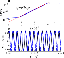
Figure 3: a: The numerically computed mean-square displacement as a function of time. The red line is the predicted exponential growth from the linear instability, $a_{0}e^{2\omega_{i}t}$, with $a_{0}$ being fitted. b: a blow up of the growth of the mean-square displacement. The black line is the exponential oscillatory instability prediction, $a_{0}e^{2\omega_{i}t}[\sin(\omega_{r}t+\psi)]^{2}$, with $\psi$ fitted.

Indeed, we see in Fig. 3 that $M(t)$ shoots up in time about sixteen orders of magnitude with exponential rate and oscillatory form precisely as predicted by the linear instability. We have also checked that the rotational contribution to $M(t)$ is negligible. We notice that the instability dominates the response after a short transient; this is consistent with the fact that the first modes contributing to the mean square displacement are high frequency stable modes.

Finally, we focus on the virial component of the shear stress $\sigma_{xy}=-\frac{1}{L^{2}}\sum_{i\neq j}^{N}r^{x}_{ij}F_{ij}^{y}$. During the development of the instability, the stress change is predicted to evolve as $\sigma_{xy}(t)-\sigma_{xy}(0)\propto e^{\omega_{i}t}\sin(\omega_{r}t+\psi)$.

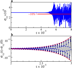
Figure 4: a: the evolution of shear stress (virial contribution) $\sigma_{xy}$ during Newtonian dynamics. The instability occuring at $t\approx 5\times 10^{5}$ results in a significant drop of the average stress. b: blow up of the stress change during the development of the instability. The black line is the theoretical prediction, $\Delta\sigma e^{\omega_{i}t}\sin{\omega_{r}t}$, with a fitted $\Delta\sigma$; the red lines mark the envelope $\pm\Delta\sigma e^{\omega_{i}t}$.

Fig. 4a shows that the stress follows the predicted linear instability with its exponential growth and oscillations until the perturbation self-amplifies enough to induce a major plastic instability in which the system undergoes a micro earthquake and loses $\simeq 10\%$ of the stress.

Taken together, Figs 2a, 3a and 4a indicate that the predictability of the evolution under the effect of the oscillatory exponential instability terminates at a time $t\approx 5\times 10^{5}$. Around that time the perturbation amplified enough for the system to switch on a non-linear response characterized by the coexistence of a number of unstable modes, saturating the mean square displacement, and causing large stress fluctuations which eventually result in a significant stress drop, cf. Fig. 4.

At this point is is important to stress that the existence of the oscillatory instability is not limited to the particular choice of forces Eqs. (6) and (7). Any reasonable coarse grained theory of tangential forces must take into account the fact that compressed granules will create a larger area of contact. Accordingly, it is expected that the tangential force will be a function not only of the $\theta_{i}$ coordinates but also of the positional coordinates ${\bm{r}}_{i}$. Consequently, in general the forces would not be derivable from a Hamiltonian, and the corresponding operator ${\bm{J}}$ will not be symmetric. There is therefore a generic possibility to find complex eigenpairs in this operator in any reasonable coarse-grained theory of frictional matter.

Having this genericity in mind, we would like to cautiously speculate about the relevance of the findings reported above to the physics of earthquakes. We of course do not propose that the system studied above of frictional disks includes all the rich physics of the earth and its faults. Nevertheless it is tempting to consider one of the most striking observation in earthquake physics which is known as “remote triggering” Felzer and Brodsky (2006); Brodsky et al. (2000); Brodsky and van der Elst (2014): an earthquake could trigger a subsequent earthquake on a different fault, even if located far away. It is clear that faults can ‘communicate’ via seismic waves propagating through the earth crust. Specifically, distant faults can only communicate via long wavelength seismic waves, as short wavelengths are quickly damped as they propagate. However seismic waves with long wavelengths act as small perturbations, as they have a small frequency and hence a small energy density, so that it is not clear how they could be able to induce the failure of a fault. The most popular approach to rationalize this observation within the geophysical community, is the acoustic fluidization Melosh (1996); Giacco et al. (2015) mechanism. This mechanism was invoked to rationalize remote triggering, suggesting that long wavelengths impacting on a fault trigger short wavelengths within the fault, and that these act by reducing the confining pressure and promoting failure. However, a detailed micromechanical investigation of this process is lacking. We would like to propose that the mechanism discussed in this Letter might be relevant for the discussion of remote triggering. Admittedly, our model system is too simple to resemble a geological fault. We propose however that the mechanism that we highlight here is generic in mechanical systems that are frictional and their dynamics is not derivable from a Hamiltonian. The crucial observation is that we have a clear mechanism for the self-amplification of small perturbations, making it quite worthwhile to study this mechanism also in the context of fault dynamics and in other context of frictional granular matter.

I Supplementary Material

The operator ${{\bm{J}}}$ involves controlling the time evolution of the system involves the derivative of the forces and of the torques acting on the particles with respect to the degree of freedom. In this supplementary notes, we first describe the interaction forces (Sec. II).The tangential force depends on a tangential displacement, whose dependence on the degree of freedom is detailed in (Sec. III). Finally, we consider the different derivatives forces as needed to evaluate the operator ${{\bm{J}}}$ in Sec. IV.

II Interaction force 

In our simulation, a pair of granular particles interacts when they overlap. The overlap distance $\delta_{ij}$ is measured as

$$\delta_{ij}=\sigma_{i}+\sigma_{j}-r_{ij},$$ (9)

where $r_{ij}$ is the center-to-center distance of a pair-$i$ and $j$, and $\sigma_{i}$ is the radius of particle-$i$. The pair vector ${{\bm{r}}}_{ij}$ is defined as

$${{\bm{r}}}_{ij}={\bm{r}}_{i}-{\bm{r}}_{j}.$$ (10)

The pair-interaction force ${{\bm{F}}}_{ij}$ has two contributions. ${{\bm{F}}}^{n}_{ij}$ is the force acting along the normal direction of the pair $\hat{r}_{ij}$, and ${{\bm{F}}}^{t}_{ij}$ is the force acting along the tangential direction of the pair ${\hat{t}}_{ij}$. The normal force is Hertzian:

$${{\bm{F}}}^{n}_{ij}=k_{n}\delta^{3/2}_{ij}{\hat{r}}_{ij},$$ (11)

where $k_{n}$ is the force constant with dimension: Force per length^3/2. The tangential force ${{\bm{F}}}^{t}_{ij}$ is a function of both the overlap distance $\delta_{ij}$ and the tangential displacement ${{\bm{t}}}_{ij}$. We have modified the standard expression for ${{\bm{F}}}^{t}_{ij}$ and included a few higher order terms of $t_{ij}$ (i.e., $|{{\bm{t}}}_{ij}|$) such that the derivative of the force function $F^{t}_{ij}$ with respect to tangential distance $t_{ij}$ becomes continuous and it goes to zero smoothly. We use the following form:

$$\begin{split}{{\bm{F}}}^{t}_{ij}&=-k_{t}\delta^{1/2}_{ij}\left[1+\frac{t_{ij}}{t^{*}_{ij}}-\left(\frac{t_{ij}}{t^{*}_{ij}}\right)^{2}\right]t_{ij}{\hat{t}}_{ij}\\ &=-k_{t}\delta^{1/2}_{ij}t^{*}_{ij}{\hat{t}}_{ij},\ \ \ \textrm{if}\ \ k_{t}\delta^{1/2}_{ij}t_{ij}>\mu|{{\bm{F}}}^{n}_{ij}|,\end{split}$$ (12)

where $k_{t}$ is the tangential force constant. Its dimension is force per length^3/2. $t^{*}_{ij}$ is the threshold tangential distance:

$$t^{*}_{ij}=\mu\frac{k_{n}}{k_{t}}\delta_{ij},$$ (13)

where $\mu$ is the friction coefficient, a scalar quantity, which essentially determines the maximum strength of the tangential force with respect to the normal force at a fixed overlap $\delta_{ij}$. The derivative of $F^{t}_{ij}$ with respect to $t_{ij}$ vanishes at $t^{*}_{ij}$, as it turns out

$$\begin{split}\frac{\partial F^{t}_{ij}}{\partial t_{ij}}&=k_{t}\delta^{1/2}_{ij}\left[1+2\frac{t_{ij}}{t^{*}_{ij}}-3\left(\frac{t_{ij}}{t^{*}_{ij}}\right)^{2}\right]\\ &=0,\ \ \ \textrm{if}\ \ k_{t}\delta^{1/2}_{ij}t_{ij}>\mu|{{\bm{F}}}^{n}_{ij}|.\end{split}$$ (14)

We stress here that the above forces imply a non Hamiltonian dynamics. That is, there is not a function $U(\delta,t)$ such that $F_{n}=-\frac{\partial U}{\partial\delta}$ and $F_{t}=-\frac{\partial U}{\partial t}$.

III Tangential displacement:

The computation of the operator ${{\bm{J}}}$ involves derivatives of the tangential force with respect to the degrees of freedom, e.g. $\frac{\partial{F^{t}_{ij}}^{\beta}}{\partial r^{\alpha}_{i}}$. Since the tangential force is expressed in terms of the tangential displacement ${\bm{t}}$, using the chain rule we will express these derivatives in terms of $\frac{\partial{t_{ij}}^{\beta}}{\partial r^{\alpha}_{i}}$. Here we evaluate these derivatives.

The derivative of tangential displacement ${{\bm{t}}}_{ij}$ with respect to time $t$ is

$$\frac{\mathrm{d}{{\bm{t}}}_{ij}}{\mathrm{d}t}={{\bm{v}}}_{ij}-{{\bm{v}}}^{n}_{ij}+\hat{r}_{ij}\times(\sigma_{i}{{\bm{\omega}}}_{i}+\sigma_{j}{{\bm{\omega}}}_{j}),$$ (15)

where ${{\bm{v}}}_{ij}={{\bm{v}}}_{i}-{{\bm{v}}}_{j}$ is the relative velocity of pair-$i$ and $j$. ${{\bm{v}}}^{n}_{ij}$ is the projection of ${{\bm{v}}}_{ij}$ along the normal direction $\hat{r}_{ij}$. ${{\bm{v}}}_{ij}-{{\bm{v}}}^{n}_{ij}$ is the tangential component of the relative velocity. ${{\bm{\omega}}}_{i}$ and ${{\bm{\omega}}}_{j}$ are the angular velocity of $i$ and $j$, respectively. In differential form, the above equation reads:

$$\mathrm{d}{{\bm{t}}}_{ij}=\mathrm{d}{{\bm{r}}}_{ij}-(\mathrm{d}{{\bm{r}}}_{ij}\cdot\hat{r}_{ij})\hat{r}_{ij}+\hat{r}_{ij}\times(\sigma_{i}\mathrm{d}{{\bm{\theta}}}_{i}+\sigma_{j}\mathrm{d}{{\bm{\theta}}}_{j}),$$ (16)

where $\mathrm{d}{{\bm{\theta}}}_{i}$ is the angular displacement of $i$ which follows the relation: $\mathrm{d}{{\bm{\omega}}}_{i}=\frac{\mathrm{d}{{\bm{\theta}}}_{i}}{\mathrm{d}t}$.

Here on, we assume the two-dimensional ($\bf 2D$) system. Therefore, $\omega_{i}$, and so $\theta_{i}$, only have one component along $\hat{z}$, perpendicular to the xy plane, and $\hat{r}_{ij}\times\mathrm{d}{{\bm{\theta}}}_{i}=\mathrm{d}\theta_{i}(y_{ij}\hat{x}-x_{ij}\hat{y})/r_{ij}$. This allows to write Eq. (16) as

$$\mathrm{d}t^{\alpha}_{ij}=\mathrm{d}r^{\alpha}_{ij}-(\mathrm{d}{{\bm{r}}}_{ij}\cdot\hat{r}_{ij})\frac{r^{\alpha}_{ij}}{{r}_{ij}}+(-1)^{\alpha}(\sigma_{i}\mathrm{d}\theta_{i}+\sigma_{j}\mathrm{d}\theta_{j})\frac{r^{\beta}_{ij}}{{r}_{ij}},$$ (17)

where $\alpha$ and $\beta$ can take value 0 and 1 which correspond to x and y components, respectively. Now if particle-$i$ changes its position the angular displacement remains unaffected, i.e. $\frac{\mathrm{d}\theta_{i}}{\mathrm{d}r^{\alpha}_{i}}=0$. Thus, the change in tangential displacement along $\beta$ due to the change in position of particle-$i$ along $\alpha$ only contributes in translations, and it can be written as (using (17))

$$\frac{\mathrm{d}t^{\beta}_{ij}}{\mathrm{d}r^{\alpha}_{i}}=\Delta_{\alpha\beta}-\frac{r^{\alpha}_{ij}r^{\beta}_{ij}}{{r}^{2}_{ij}},$$ (18)

where $\Delta_{\alpha\beta}$ is the Kronecker delta which is one when $\alpha=\beta$, or else zero. Similarly, a change in rotational coordinates does not modify the particles relative distance, i.e. $\frac{\mathrm{d}r^{\beta}_{ij}}{\mathrm{d}\theta_{i}}=0$. Thus, the change in tangential displacement along $\beta$ due to the change in $\theta_{i}$ is (from (17))

$$\frac{\mathrm{d}t^{\beta}_{ij}}{\mathrm{d}\theta_{i}}=(-1)^{\beta}\sigma_{i}\frac{r^{\alpha}_{ij}}{{r}_{ij}}.$$ (19)

In the above equation $\alpha$ and $\beta$ are always different. Now the magnitude of tangential distance $t_{ij}$ can be obtained from the relation $t^{2}_{ij}=\sum_{\alpha}{t^{\alpha}_{ij}}^{2}$. Its differential follows $\mathrm{d}t_{ij}=\sum_{\alpha}\frac{t^{\alpha}_{ij}}{t_{ij}}\mathrm{d}t^{\alpha}_{ij}$. The derivatives of tangential distance $t_{ij}$ with respect to $r^{\alpha}_{i}$ and $\theta_{i}$ can be expressed as

$$\frac{\mathrm{d}t_{ij}}{\mathrm{d}r^{\alpha}_{i}} = \left(\frac{t^{x}_{ij}}{t_{ij}}\right)\frac{\mathrm{d}t^{x}_{ij}}{\mathrm{d}r^{\alpha}_{i}}+\left(\frac{t^{y}_{ij}}{t_{ij}}\right)\frac{\mathrm{d}t^{y}_{ij}}{\mathrm{d}r^{\alpha}_{i}},$$ (20)

$$\frac{\mathrm{d}t_{ij}}{\mathrm{d}\theta_{i}} = \left(\frac{t^{x}_{ij}}{t_{ij}}\right)\frac{\mathrm{d}t^{x}_{ij}}{\mathrm{d}\theta_{i}}+\left(\frac{t^{y}_{ij}}{t_{ij}}\right)\frac{\mathrm{d}t^{y}_{ij}}{\mathrm{d}\theta_{i}}.$$ (21)

With the help of equations (18) and (19) we can solve the above two differential equations. As the tangential threshold is a linear function of overlap distance $\delta_{ij}$ (see (13)), it also gets modified due to a change in $r^{\alpha}_{i}$ as

$$\frac{\mathrm{d}t^{*}_{ij}}{\mathrm{d}r^{\alpha}_{i}}=-\mu\left(\frac{k_{n}}{k_{t}}\right)\frac{r^{\alpha}_{ij}}{r_{ij}},$$ (22)

and it is unaffected by the change in rotation, i.e. $\frac{\mathrm{d}t^{*}_{ij}}{\mathrm{d}\theta_{i}}=0$.

IV Evaluation of ${{\bm{J}}}$

IV.1 Derivative of tangential force

The derivative of tangential force (equation (12)) with respect to $r^{\alpha}_{i}$:

$$\frac{\partial{F^{t}_{ij}}^{\beta}}{\partial r^{\alpha}_{i}} = -k_{t}\frac{\partial}{\partial r^{\alpha}_{i}}\left[\delta^{1/2}_{ij}\left(t^{\beta}_{ij}+\tilde{t}t^{\beta}_{ij}-{\tilde{t}}^{2}t^{\beta}_{ij}\right)\right]$$ (23)

$$= -\frac{1}{2}\delta^{-1}_{ij}\frac{r^{\alpha}_{ij}}{r_{ij}}{F^{t}_{ij}}^{\beta}-k_{t}\delta^{1/2}_{ij}\left[(1+{\tilde{t}}-{\tilde{t}}^{2})\frac{\partial t^{\beta}_{ij}}{\partial r^{\alpha}_{i}}+({\tilde{t}}^{\beta}-2{\tilde{t}}{\tilde{t}}^{\beta})\frac{\partial t_{ij}}{\partial r^{\alpha}_{i}}+(-{\tilde{t}}{\tilde{t}}^{\beta}+2{\tilde{t}}^{2}{\tilde{t}}^{\beta})\frac{\partial t^{*}_{ij}}{\partial r^{\alpha}_{i}}\right]$$

Here we use the notation $\tilde{t}$ to represent the ratio $t_{ij}/t^{*}_{ij}$, and the notation ${\tilde{t}}^{\beta}$ for ${t_{ij}}^{\beta}/t^{*}_{ij}$. The expressions for all the three partial differentiation in (23) are already shown in (19), (20), and (22).

Similarly, the derivative of tangential force with respect to $\theta_{i}$ (using the same notation as above) can be found as

$$\frac{\partial{F^{t}_{ij}}^{\beta}}{\partial\theta_{i}}=-k_{t}\delta^{1/2}_{ij}\left[(1+{\tilde{t}}-{\tilde{t}}^{2})\frac{\partial t^{\beta}_{ij}}{\partial\theta_{i}}+({\tilde{t}}^{\beta}-2{\tilde{t}}{\tilde{t}}^{\beta})\frac{\partial t_{ij}}{\partial\theta_{i}}\right]$$ (24)

From the above two equations it is then understood that if ${{\bm{r}}}_{ij}$ and ${{\bm{t}}}_{ij}$ are known the differential equations can be solved easily. When ${\tilde{t}}^{\beta}$ is negligible for all $\beta$, then ${\tilde{t}}\approx 0$. This translates to $\frac{\partial{F^{t}_{ij}}^{\beta}}{\partial\theta_{i}}=-(-1)^{\beta}k_{t}\sigma_{i}\delta^{1/2}_{ij}\frac{r_{ij}^{\alpha}}{r_{ij}}$ with $\alpha\neq\beta$, implying that even in the case of zero tangential displacement and therefore, zero tangential force, the above derivative can be finite.

IV.2 Derivative of normal force

The derivative of normal force (equation (11)) with respect to $r^{\alpha}_{i}$:

$$\frac{\partial{F^{n}_{ij}}^{\beta}}{\partial r^{\alpha}_{i}} = k_{n}\frac{\partial}{\partial r^{\alpha}_{i}}\left[\delta^{3/2}_{ij}\frac{r^{\beta}_{ij}}{r_{ij}}\right]$$ (25)

$$= k_{n}\delta^{1/2}_{ij}\left[\Delta_{\alpha\beta}\frac{\delta_{ij}}{r_{ij}}-\frac{3}{2}\frac{r^{\alpha}_{ij}r^{\beta}_{ij}}{r^{2}_{ij}}-\left(\frac{\delta_{ij}}{r_{ij}}\right)\frac{r^{\alpha}_{ij}r^{\beta}_{ij}}{r^{2}_{ij}}\right],$$

where $\Delta_{\alpha\beta}$ is the Kronecker delta. The derivative of total force which reads:

$$\frac{\partial{F_{ij}}^{\beta}}{\partial r^{\alpha}_{i}} = \frac{\partial{F^{n}_{ij}}^{\beta}}{\partial r^{\alpha}_{i}}+\frac{\partial{F^{t}_{ij}}^{\beta}}{\partial r^{\alpha}_{i}}$$ (26)

$$\frac{\partial{F_{ij}}^{\beta}}{\partial\theta_{i}} = \frac{\partial{F^{t}_{ij}}^{\beta}}{\partial\theta_{i}}$$ (27)

can be solved using (25), (23), and (24).

IV.3 Derivative of Torque

The torque of particle-$j$ due to tangential force ${{\bm{F}}^{t}}_{ij}$ is ${{\bm{T}}}_{j}=-\sigma_{j}\left({\hat{r}}_{ij}\times{{\bm{F}}^{t}}_{ij}\right)\equiv\sigma_{j}\tilde{{\bm{T}}}_{ij}$. In 2D, $\tilde{{\bm{T}}}_{ij}$ has only z-component:

$${\tilde{T}}_{ij}^{z}=-\left[\left(\frac{x_{ij}}{r_{ij}}\right){F^{t}_{ij}}^{y}-\left(\frac{y_{ij}}{r_{ij}}\right){F^{t}_{ij}}^{x}\right].$$ (28)

The derivative of ${\tilde{T}}_{ij}^{z}$ then becomes:

$$\frac{\partial{\tilde{T}}_{ij}^{z}}{\partial r^{\alpha}_{i}}=-\left(\frac{\delta_{\alpha x}}{r_{ij}}-\frac{x_{ij}r_{ij}^{\alpha}}{r_{ij}^{3}}\right){F^{t}_{ij}}^{y}-\left(\frac{x_{ij}}{r_{ij}}\right)\frac{\partial{F^{t}_{ij}}^{y}}{\partial r^{\alpha}_{i}}+\left(\frac{\delta_{\alpha y}}{r_{ij}}-\frac{y_{ij}r_{ij}^{\alpha}}{r_{ij}^{3}}\right){F^{t}_{ij}}^{x}+\left(\frac{y_{ij}}{r_{ij}}\right)\frac{\partial{F^{t}_{ij}}^{x}}{\partial r^{\alpha}_{i}},$$ (29)

where $\delta_{\alpha x}$ (similarly, $\delta_{\alpha y}$) is the Kronecker delta, such that $\delta_{xx}=1$ and $\delta_{yx}=0$, and

$$\frac{\partial{\tilde{T}}_{ij}^{z}}{\partial\theta_{i}}=-\left[\left(\frac{x_{ij}}{r_{ij}}\right)\frac{\partial{F^{t}_{ij}}^{y}}{\partial\theta_{i}}-\left(\frac{y_{ij}}{r_{ij}}\right)\frac{\partial{F^{t}_{ij}}^{x}}{\partial\theta_{i}}\right]$$ (30)

The above two differential equations can be solved using (23), and (24). If the tangential displacement $t_{ij}^{\beta}$ is negligible compared to the threshold $t_{ij}^{*}$, i.e., ${\tilde{t}}^{\beta}\approx 0$ for all $\beta$. This results in ${\tilde{t}}\approx 0$. Therefore, $\frac{\partial{\tilde{T}}_{ij}^{z}}{\partial\theta_{i}}=k_{t}\sigma_{i}\delta_{ij}^{1/2}$.

IV.4 Jacobian

The dimension of Jacobian operator $J$ is force over length. To be consistent with the dimension we redefine the torque $T$ and rotational coordinate $\theta$ as

$${\tilde{T}}_{i}=\frac{T_{i}}{\sigma_{i}},\ \ \ \textrm{and}\ \ \ {\tilde{\theta}}_{i}=\sigma_{i}\theta_{i}$$ (31)

In addition, the dynamic matrix has a contribution from the moment of inertia $I_{i}=I_{0}m_{i}\sigma_{i}^{2}$ as $\Delta{{\bm{\omega}}}_{i}={{\bm{T}}}_{i}/I_{i}\Delta t$. In our calculation, we assume that mass $m_{i}$ and $I_{0}$ both are one. The remaining contribution of $I_{i}$, i.e. $\sigma_{i}^{2}$, is taken care of by rescaling the torque and the angular displacement as ${\tilde{T}}_{i}$ and ${\tilde{\theta}_{i}}$ (31). For $I_{0}\neq 1$, the contribution of $I_{0}$ can be correctly anticipated if we rewrite (15) as below:

$$\frac{\mathrm{d}{{\bm{t}}}_{ij}}{\mathrm{d}t}={{\bm{v}}}_{ij}-{{\bm{v}}}^{n}_{ij}+\frac{1}{I_{0}}\hat{r}_{ij}\times(\sigma_{i}{{\bm{\omega}}}_{i}+\sigma_{j}{{\bm{\omega}}}_{j}),$$ (32)

$J$ essentially contains four different derivatives:

• First type: Derivative of force with respect to the position of particles:

  $$\begin{split}&J^{\alpha\beta}_{ij}=\sum_{k=0;k\neq j}^{N-1}\frac{\partial F^{\beta}_{kj}}{\partial r^{\alpha}_{i}}=\frac{\partial F^{\beta}_{ij}}{\partial r^{\alpha}_{i}},\ \ \ \textrm{for}\ \ i\neq j\\ &J^{\alpha\beta}_{ii}=\sum_{j=0;j\neq i}^{N-1}\frac{\partial F^{\beta}_{ji}}{\partial r^{\alpha}_{i}}=-\sum_{j=0;j\neq i}^{N-1}J^{\alpha\beta}_{ij},\end{split}$$ (33)

  where $N$ is the total number of particles. $J^{\alpha\beta}_{ij}$ is symmetric if we change pairs, i.e.: $J^{\alpha\beta}_{ij}=J^{\alpha\beta}_{ji}$, however the symmetry is not guaranteed with the interchange of $\alpha$ and $\beta$.

• Second type: Derivative of force with respect to rotational coordinate:

  $$\begin{split}&J^{\beta}_{ij}=-\sum_{k=0;k\neq j}^{N-1}\frac{\partial F^{\beta}_{kj}}{\partial\tilde{\theta}_{i}}=-\frac{\partial F^{\beta}_{ij}}{\partial\tilde{\theta}_{i}},\ \ \ \textrm{for}\ \ i\neq j\\ &J^{\beta}_{ii}=-\sum_{j=0;j\neq i}^{N-1}\frac{\partial F^{\beta}_{ji}}{\partial\tilde{\theta}_{i}}=\sum_{j=0;j\neq i}^{N-1}J^{\beta}_{ij}.\end{split}$$ (34)

  The negative sign makes sure that in stable systems all the eigenvalues are positive. $J^{\beta}_{ij}$ is asymmetric: $J^{\beta}_{ij}=-J^{\beta}_{ji}$.

• Third type: Derivative of torque with respect to position:

  $$\begin{split}&J^{\alpha}_{ij}=\sum_{k=0;k\neq j}^{N-1}\frac{\partial{\tilde{T}}_{kj}^{z}}{\partial r^{\alpha}_{i}}=\frac{\partial{\tilde{T}}_{j}}{\partial r^{\alpha}_{i}},\ \ \ \textrm{for}\ \ i\neq j\\ &J^{\alpha}_{ii}=\sum_{j=0;j\neq i}^{N-1}\frac{\partial{\tilde{T}}_{ji}^{z}}{\partial r^{\alpha}_{i}}=\sum_{j=0;j\neq i}^{N-1}J^{\alpha}_{ij}.\end{split}$$ (35)

  $J^{\alpha}_{ij}$ is also asymmetric: $J^{\alpha}_{ij}=-J^{\alpha}_{ji}$.

• Fourth type: Derivative of torque with respect to rotational coordinate:

  $$\begin{split}&J_{ij}=-\sum_{k=0;k\neq j}^{N-1}\frac{\partial{\tilde{T}}_{kj}^{z}}{\partial\tilde{\theta}_{i}}=-\frac{\partial{\tilde{T}}_{j}}{\partial\tilde{\theta}_{i}},\ \ \ \textrm{for}\ \ i\neq j\\ &J_{ii}=-\sum_{j=0;j\neq i}^{N-1}\frac{\partial{\tilde{T}}_{ji}^{z}}{\partial\tilde{\theta}_{i}}=-\sum_{j=0;j\neq i}^{N-1}J_{ij}.\end{split}$$ (36)

  The negative sign makes sure that in stable systems all the eigenvalues are positive. $J_{ij}$ is symmetric: $J_{ij}=J_{ji}$.

IV.5 Arrangement of Jacobian matrix

In two dimension $D=2$, for $N$ particles the total number of elements in $J$ is $(D+1)N\times(D+1)N$. In the matrix, first $DN\times DN$ elements contain the first type of force derivative, i.e. $J^{\alpha\beta}_{ij}$. Here the row-index $ro$ and column-index $co$ of $J$ runs in the range $0\leq ro<DN$ and $0\leq co<DN$. Rows from $DN\leq ro<(D+1)N$ and columns $0\leq co<DN$ of $J$ contain $J^{\beta}_{ij}$, i.e., the second type of derivative. Rows from $0\leq ro<DN$ and columns $DN\leq co<(D+1)N$ of $J$ contain the third type $J^{\alpha}_{ij}$. Finally, rows from $DN\leq ro<(D+1)N$ and columns $DN\leq co<(D+1)N$ of $J$ hold $J_{ij}$, i.e., the fourth type of derivative. For a fixed type of derivative, at a fixed row, the column-index first runs over $j$ starting from 0 to $N-1$. Then $\beta$ is incremented, if it exists for that particular derivative type. Similarly, at a fixed column, row-index first runs over $i\in[0,N)$ and then $\alpha$ is incremented.

References

Liu and Nagel (1998)
A. Liu and
S. Nagel,
Nature 396, 21
(1998).
O’Hern et al. (2001)
C. S. O’Hern,
S. A. Langer,
A. J. Liu, and
S. R. Nagel,
Phys. Rev. Lett. 86,
111 (2001).
Wyart, M. (2005)
Wyart, M., Ann. Phys. Fr.
30, 1 (2005).
Berthier and Biroli (2011)
L. Berthier and
G. Biroli,
Rev. Mod. Phys. 83,
587 (2011).
Ciamarra et al. (2011)
M. P. Ciamarra,
R. Pastore,
M. Nicodemi, and
A. Coniglio,
Phys. Rev. E 84,
041308 (2011).
Malandro and Lacks (1998)
D. L. Malandro and
D. J. Lacks,
Phys. Rev. Lett. 81,
5576 (1998).
Malandro and Lacks (1999)
D. L. Malandro and
D. J. Lacks,
J. Chem. Phys p. 4593
(1999).
Maloney and Lemaître (2004)
C. Maloney and
A. Lemaître,
Physi. Rev. Lett. 93,
195501 (2004).
Karmakar et al. (2010)
S. Karmakar,
E. Lerner, and
I. Procaccia,
Phys. Rev.E 82,
026105 (2010).
Mizuno et al. (2017)
H. Mizuno,
H. Shiba, and
A. Ikeda,
Proceedings of the National Academy of Sciences of the
United States of America 114,
E9767 (2017).
Hentschel et al. (2011)
H. G. E. Hentschel,
S. Karmakar,
E. Lerner, and
I. Procaccia,
Phys. Rev.E 83,
061101 (2011).
Procaccia et al. (2016)
I. Procaccia,
C. Rainone,
C. A. B. Z. Shor,
and M. Singh,
Phys. Rev.E 93
(2016).
Dailidonis et al. (2017)
V. Dailidonis,
V. Ilyin,
I. Procaccia,
and C. A. B. Z.
Shor, Phys. Rev. E
95, 031001
(2017).
Dasgupta et al. (2012)
R. Dasgupta,
H. G. E. Hentschel,
and
I. Procaccia,
Phys. Rev. Lett. 109,
255502 (2012).
Dasgupta
et al. (2013a)
R. Dasgupta,
H. G. E. Hentschel,
and
I. Procaccia,
Phys. Rev.E 87,
022810 (2013a).
Dasgupta
et al. (2013b)
R. Dasgupta,
O. Gendelman,
P. Mishra,
I. Procaccia,
and C. A. Shor,
Phys. Rev.E 88,
032401 (2013b).
Mindlin (1949)
R. Mindlin,
Trans. ASME 16,
259 (1949).
Silbert et al. (2001)
L. E. Silbert,
D. Ertaş, G. S. Grest,
T. C. Halsey,
D. Levine, and
S. J. Plimpton,
Phys. Rev. E 64,
051302 (2001).
Zhang and Makse (2005)
H. Zhang and
H. A. Makse,
Physical Review E 72,
011301 (2005).
Plimpton (1995)
S. Plimpton,
Journal of Computational Physics
117, 1 (1995).
Felzer and Brodsky (2006)
K. Felzer and
E. Brodsky,
Nature 441,
735–738 (2006).
Brodsky et al. (2000)
E. E. Brodsky,
V. Karakostas,
and H. Kanamori,
Geophysical Research Letters
27, 2741 (2000).
Brodsky and van der Elst (2014)
E. E. Brodsky and
N. J. van der Elst,
Annual Review of Earth and Planetary Sciences
42, 317 (2014).
Melosh (1996)
H. Melosh,
Nature 379,
601 (1996).
Giacco et al. (2015)
F. Giacco,
L. Saggese,
L. De Arcangelis,
E. Lippiello,
and M. Pica
Ciamarra, Physical Review Letters
115, 128001
(2015).