The semi-algebraic geometry of saturated optimal designs for the Bradley–Terry model

Abstract.

Optimal design theory for nonlinear regression studies local optimality on a given design space. We identify designs for the Bradley–Terry paired comparison model with small undirected graphs and prove that every saturated, locally $D$-optimal design is represented by a path. We discuss the case of four alternatives in detail and derive explicit polynomial inequality descriptions for optimality regions in parameter space. Using these regions, for each point in parameter space we can prescribe a locally $D$-optimal design.

Key words and phrases: nonlinear regression, optimal design, polynomial inequalities

1. Introduction

Consider an experimental situation in which $m$ alternatives are to be brought into a rank order. For each single observation in this experiment only two of these alternatives can be compared at a time and only a binary response can be observed which indicates the rank order of the two alternatives presented. Such experiments are known in economics as “discrete choice” experiments and in psychology as “forced choice” experiments or “ipsative measures”. The use of such experiments dates back to the work by Fechner [Fec66] on psychophysics in a deterministic setup. In a statistical setup this situation is described by the Bradley-Terry model, which was introduced in [Zer29] to rank chess players in tournaments and in [BT52] to analyze taste testing results for pork depending on different feeding patterns. See [KRS20] for a leisurely introduction. This model has proven popular in different areas of statistics, also outside of chess tournaments and pork tasting. In [HT98], Hastie and Tibshirani developed a coupling model similar to the Bradley–Terry model to study class probabilities for pairs of classes. [SY99] discussed the model asymptotics when the number of potential alternatives tends to infinity. Algorithms for Bradley–Terry models are discussed, for example, in [Hun04], and asymptotics of algorithms, for example, in [DMJ13]. Besides marketing or transportation, another popular application area for the Bradley–Terry model is the world of professional sports such as American football, car racing, matching in tournaments, card games or strategies for sport bets, see [CMP07, GRF03, BMS04, KKT06]. The Bradley–Terry model is part of a broader class of models that describe statistical rankings. Specifically, it arises from marginalization of the Plackett–Luce model, see [SW12].

In this paper we are interested in optimal experimental designs for the Bradley–Terry model, that is, a scheme to assign a fixed number of measurements to different experimental settings, such that the experiment is most informative about the parameters. Optimal experimental designs for the Bradley–Terry model were first investigated in [Tor04], which gave an algorithmic approach to fit the model parameters. In [GS08] Graßhoff and Schwabe completely analyzed the case of three competing alternatives (with pair comparisons). They gave symbolic solutions for the design problem depending on the parameters and described the optimality areas of these design classes in the parameter space. The present paper extends the results of Graßhoff and Schwabe in two directions. We discuss the case of four competing alternatives in detail and characterize optimal saturated designs for an arbitrary number of competing alternatives, always with pair comparisons. The case of four alternatives arises also when considering a $2^{2}$ layout with interaction where two attributes can be set to two levels each. After a reparametrization, which does not affect the $D$-optimality, this model can be identified as a single-attribute model with four levels which can be used as alternatives in the Bradley–Terry model.

Section 2 gives the general setup. Section 5 contains an almost complete analysis of the case of 4 alternatives. Only one very challenging polynomial inequality system remains open (Problem 15). In Sections 3 and 4 we discuss saturated optimal designs for an arbitrary number of alternatives. Our main result is an easy combinatorial polynomial inequality description of regions in parameter space where a given saturated design is optimal, including the information for which designs these regions of optimality are empty (Theorem 11). Polynomial inequality constraints in experimental design are a recurrent topic. See [KOS16] for a discussion of this principle for Poisson regression. Knowledge about the optimality regions can be very helpful in designing experiments. For example, a screening experiment could reveal that the estimates of the parameters are all within one region of optimality. In such a situation it is then clear which design to use. See [DMP04] for a general class of models where local optimality is studied. In the discussion in Section 6 we compare the efficiency of our tailored designs versus uniform designs as the parameters grow in magnitude.

2. General Setup

We consider pairs $(i,j)$ of alternatives $i,j=1,\ldots,m$. The preference of $i$ over $j$ is modeled by a binary variable $Y(i,j)$ taking the value $Y(i,j)=1$ if $i$ is preferred over $j$ and $Y(i,j)=0$ otherwise. We do not consider any order effects here. The main assumption of the Bradley–Terry model is that there is a hidden ranking of the alternatives according to some numerical preference value $\pi_{i}>0$, $i=1,\dots,m$. When presented with the pair $(i,j)$, the probability of preferring $i$ over $j$ is

$$\mathbb{P}(Y(i,j)=1)=\frac{\pi_{i}}{\pi_{i}+\pi_{j}}.$$

The model can be transformed into a logistic model using $\beta_{i}:=\log(\pi_{i})$. Then

$$\mathbb{P}(Y(i,j)=1)=\frac{1}{1+\exp(-(\beta_{i}-\beta_{j}))}=\eta(\beta_{i}-\beta_{j})$$

with $\eta(z)=(1+\exp(-z))^{-1}$ as the inverse logit link function.

Scaling all $\pi_{i}$ with a constant factor leaves the preference probabilities invariant. Therefore one can without loss of generality assume that $\pi_{m}=1$ or $\beta_{m}=0$. This means that the number of parameters of the Bradley–Terry model is $m-1$. The number of alternatives is the main measure of complexity of the design theory as it equals the dimension of the design space. The remaining parameters can be identified and $\beta_{m}=0$ is known as control coding. We denote by $e_{i}$ the $i$-th standard unit vector in $\mathbb{R}^{m-1}$. To exhibit our model as a generalized linear model, the regression vector for a pair $(i,j)$ is

$$f(i,j)=\begin{cases}e_{i}-e_{j},&\text{for }i,j\neq m,\\ e_{i},&\text{for }i<j,j=m,\\ 0&\text{for }i=j=m.\end{cases}$$

With $\beta^{T}=(\beta_{1},\ldots,\beta_{m-1})$ this yields $\mathbb{P}(Y(i,j)=1)=\eta(f(i,j)^{T}\beta)$ where $f(i,j)^{T}\beta$ is the linear predictor.

Remark 1.

When all probabilities

$$p_{ij}:=\mathbb{P}(Y(i,j)=1)=\frac{\pi_{i}}{\pi_{i}+\pi_{j}}~{}~{}\text{ for }i,j\in[m]:=\{1,2,\ldots,m\}$$

are treated as coordinates in $\mathbb{R}^{m(m-1)}$, the Bradley–Terry model can be described by algebraic equations. This means that all values of the $p_{ij}$ that arise for different values of $\pi$ satisfy certain algebraic equations and, among the probability vectors, they are the only solutions to these equations. Theorem 7.7 of [SW12] shows that the model has the special geometric structure of a toric variety and its defining equations consist of binomials and linear trinomials.

The design region of the Bradley–Terry paired comparison model is

$$\mathcal{X}=\{(i,j)\,:\,i,j=1,...,m,\,i<j\}.$$

It consists of all pairs of ordered alternatives. The pairs $(i,j)$ and $(j,i)$ bear the same information, and the comparison $(i,i)$ of two identical alternatives does not have any information at all (as can be seen easily later). Therefore, whenever there are two alternatives $i,j\in\{1,\dots,m\}$ we assume $i<j$. An experimental design is an assignment of a weight $w_{ij}\geq 0$ to each point $(i,j)\in\mathcal{X}$, such that $\sum_{ij}w_{ij}=1$ (compare, for example, [Sil80]). Although a design could be impossible to realize with a finite number $N$ of observations, it is common to let $w_{ij}\in\mathbb{R}$ as opposed to $w_{ij}\in\frac{1}{N}\mathbb{N}$. For any $k\in\mathbb{N}$ we write

$$\Delta_{k}:=\{w\in\mathbb{R}^{k}_{\geq 0}:\sum_{l}w_{l}=1\},$$

for the $k-1$ dimensional simplex in $\mathbb{R}^{k}$, whose vertices are the standard unit vectors. It is customary to use $\xi$ to refer to a design with weights $w_{ij}$ and slightly abuse notation with expressions like $\xi\in\Delta_{\binom{m}{2}}$.

The information gained from one observation of $Y(i,j)$ is encoded in the information matrix

$$M((i,j),\beta)=\lambda_{ij}f(i,j)f(i,j)^{T}\in\mathbb{R}^{(m-1)\times(m-1)},$$

where

$$\lambda_{ij}:=\lambda_{i,j}(\beta)=\eta^{\prime}(\beta_{i}-\beta_{j})=\frac{e^{\beta_{i}-\beta_{j}}}{(1+e^{\beta_{i}-\beta_{j}})^{2}}$$

is referred to as the intensity in [GS08]. It holds that $M((i,j),\beta)=M((j,i),\beta)$ and $M((i,i),\beta)=0$.

Assuming independent observations, the information matrix for a design $\xi$ with weights $w_{ij}$ is the $(m-1)\times(m-1)$-matrix

(2.1) $$M(\xi,\beta)=\sum_{(i,j)}w_{ij}M((i,j),\beta)=\sum_{(i,j)}w_{ij}\lambda_{ij}f(i,j)f(i,j)^{T}.$$

The theory of optimal experimental design suggests picking weights $w_{ij}$ that optimize a numerical function of $M(\xi,\beta)$. Standard references that include the theory for generalized linear models are [Puk06, Sil80]. One popular function to optimize is the logarithm of the determinant:

Definition 2.

An experimental design $\xi^{*}$ is locally $D$-optimal, if

$$\log\det(M(\xi^{*},\beta))\geq\log\det(M(\xi,\beta))$$

for all $\xi\in\Delta_{{\binom{m}{2}}}$.

In optimal experimental design one speaks of local optimality if the optimal choice of a design depends on the unknown parameters that one wants to learn about, see  [Che53]. From the perspective of mathematical optimization one has a parametric family of convex optimization problems where both the optimization domain (the polytope of information matrices) and the target function depend on the parameters $\beta$. The methods of convex optimization suggest studying the directional derivatives of the target function. The following is found in [Sil80, Section 3.5.2].

Definition 3.

The directional derivative (Fréchet derivative) of the $D$-optimality criterion at $M_{1}$ in the direction of $M_{2}$ for some $(m-1)\times(m-1)$ information matrices $M_{1},M_{2}$ is

$$F_{D}(M_{1},M_{2})=\lim_{\varepsilon\searrow 0}\frac{1}{\varepsilon}\left(\log\det((1-\varepsilon)M_{1}+\varepsilon M_{2})-\log\det(M_{1})\right).$$

It is shown in [Sil80, Sections 3.8 and 3.11] that

(2.2) $$F_{D}(M(\xi,\beta),M((i,j),\beta))=\lambda_{ij}f(i,j)^{T}M(\xi,\beta)^{-1}f(i,j)-(m-1).$$

This yields the following $D$-optimality criterion:

Theorem 4 (Kiefer–Wolfowitz).

A design $\xi^{*}$ is locally $D$-optimal if and only if

(2.3) $$\lambda_{ij}f(i,j)^{T}M(\xi^{*},\beta)^{-1}f(i,j)\leq m-1$$

for all $1\leq i<j\leq m$ .

The following corollary from [Sil80, Corollary 3.10] is very useful.

Corollary 5.

For design points $(i,j)$ with positive weight in $\xi^{*}$, the inequalities (2.3) in Theorem 4 hold with equality.

A main observation about the Bradley–Terry model is that it is useful to represent pairs $(i,j)$ with positive weights $w_{ij}$ as the edges of an undirected graph on the vertex set $\{1,\dots,m\}$. Properties of these graphs, in particular the edge density, determine the asymptotics of estimation for sparse Bradley–Terry models [HYTC20].

Definition 6.

A graph representation of a design $\xi$ for the Bradley–Terry model is the undirected simple graph with vertex set $\{1,\dots,m\}$, and edge set $E=\{(i,j):w_{ij}>0\}$.

Using standard notions from graph theory, a tree is a connected graph with no cycles. A path is a tree in which every vertex is connected to at most two other vertices. We exploit the symmetry of the model. The symmetric group $S_{m}$ of all bijective self-maps of $\{1,\dots,m\}$ permutes the alternatives. The permutation action extends to ordered pairs by acting on both entries of the pair simultaneously (and changing the order if necessary). The action also extends naturally to designs $\xi$ on pairs $(i,j)$ by putting $(\xi^{\sigma})_{(i,j)}=\xi_{\sigma^{-1}(i,j)}$ for any $\sigma\in S_{m}$. A graph representation of an entire orbit under this action is simply the unlabeled graph. Proposition 7 below expresses that for properties of the model it is irrelevant which alternative is alternative 1, which is alternative 2 and so on. One only needs to take care that upon relabeling the parameters, regression vectors, etc. are relabeled accordingly.

In our setup we have singled out the last alternative $m$ and set $\beta_{m}=0$ to have identifiable parameters. This changes the symmetry and needs to be accounted for. The concepts of this paper, however, are compatible with this. For example the value of the determinant of a design is equivariant:

Proposition 7.

Let $\sigma\in S_{m}$ and let $\xi$ be any design. Then $\xi$ is locally $D$-optimal for the parameters $\beta^{T}=(\beta_{1},\dots,\beta_{m-1})$ if and only if $\xi^{\sigma}$ is locally $D$-optimal for $Q_{\sigma}^{-T}\beta$, where $\sigma\mapsto Q_{\sigma}$ is a group homomorphism from $S_{m}$ to the group of invertible $(m-1)\times(m-1)$-matrices satisfying $f(\sigma(i),\sigma(j))=Q_{\sigma}f(i,j)$ for all $\sigma\in S_{m}$.

Proof.

By [RS16, Section 2], the design $\xi^{\sigma}$ is locally optimal for the parameter $Q_{\sigma}^{-T}\beta$ if and only if there exist matrices $Q_{\sigma}$ as in the statement. As transpositions generate all permutations, it suffices to show the existence of such a $Q_{\sigma}$ for all transpositions. For transpositions of $i<m$ and $j<m$, let $Q_{\sigma}$ be the usual permutation matrix. For a transposition $(im)$, let $Q_{\sigma}$ equal an identity matrix, with the $i$-th row replaced by the row $(-1\ldots,-1)$. Then, for an arbitrary permutation $\sigma$, it holds that $f(\sigma(i),\sigma(j))=Q_{\sigma}f(i,j)$. ∎

3. Saturated designs and graph-representation

An experimental design is saturated if its support has cardinality equal to the number of free parameters of the model. In our case of $D$-optimality, if a design has support size strictly smaller than $m-1$, the determinant of the information matrix vanishes and optimality is impossible. A useful result about saturated designs is that their weights are completely rigid: they are all equal [Sil80, Lemma 5.1.3] and thus only the different supports are considered. We first study which saturated designs can be $D$-optimal. The following simple fact is reminiscent of the connectedness of block designs with block length two in [SS89, p.2].

Lemma 8.

For any locally $D$-optimal saturated design $\xi$ of the Bradley–Terry paired comparison model, the graph representation of the support is a tree.

Proof.

A saturated design consists of $m-1$ equally weighted comparisons. If there is a cycle $i_{1},\dots,i_{k}$ in the graph representation of the design, then there is at least one alternative that does not appear in the design and therefore is represented by a disconnected vertex in the graph representation. Now, the $(m-1)\times(m-1)$-information matrix of a saturated design is a sum of $m-1$ rank one matrices of the form $\lambda_{ij}f(i,j)f(i,j)^{T}$. For $1\leq i<j\leq m-1$, these rank one matrices only have entries in the $i$-th and $j$-th rows and columns. For $j=m$, there is only one entry $\lambda_{im}$ in the intersection of the $i$-th row and $i$-th column. Thereby, if a saturated design contains a cycle and misses one alternative that is not $m$, the information matrix has no non-zero entries in either the corresponding row or the corresponding column. If alternative $m$ is missed, it follows that every row sum of the information matrix is zero, as all rank one matrices are of the form $\lambda_{ij}(e_{i}-e_{j})(e_{i}-e_{j})^{T}$. Therefore the determinant of the information matrix is zero, and the design can never be optimal. ∎

Based on this fact we can determine the saturated optimal designs for the Bradley–Terry model.

Theorem 9.

In the Bradley–Terry paired comparison model with $m$ alternatives, if a design is saturated and locally D-optimal, then its graph representation is a path on $[m]:=\{1,2,\ldots,m\}$.

Proof.

Let $\xi$ be a saturated, locally $D$-optimal design for the Bradley–Terry model with $m$ alternatives. The graph representation of $\xi$ is a tree by Lemma 8. Applying a suitable permutation of $[m]$ and Proposition 7, we assume that $\xi$ has exactly one comparison that contains $m$, that is, that $m$ is a leaf. Let $F$ be the (square) matrix of the transposed regression vectors of the design points

$$F=\begin{pmatrix}f(i_{1},j_{1})^{T}\\ f(i_{2},j_{2})^{T}\\ \vdots\\ f(i_{m-2},j_{m-2})^{T}\\ f(i_{m-1},m)^{T}\\ \end{pmatrix},$$

and define $Q=\text{diag}(\lambda_{i_{1},j_{1}},\dots,\lambda_{i_{m-1},m})$ as a diagonal matrix of intensities and correspondingly $W=\text{diag}(w_{i_{1},j_{1}},\dots,w_{i_{m-1},m})$ for the weights of the design points. Then, the information matrix is $M(\xi,\beta)=F^{T}WQF,$ and inserting this into (2.2), we obtain the directional derivatives for every $1\leq i<j\leq m-1$ as

$$\lambda_{ij}f(i,j)^{T}F^{-1}Q^{-1}W^{-1}F^{-T}f(i,j)-(m-1).$$

If the design is $D$-optimal, this formula is non-positive for every $1\leq i<j\leq m-1$. Since all weights are equal to $\frac{1}{m-1}$ this is equivalent to

$$\lambda_{ij}f(i,j)^{T}F^{-1}Q^{-1}F^{-T}f(i,j)\leq 1.$$

The proof is by downward induction. To this end, we remove one alternative and its associated design point and show that the reduced design $\bar{\xi}$ is optimal on the reduced design space. Without loss of generality we can assume that the optimal design has only one comparison $(1,v)$ in which alternative $1$ is involved. We can also assume that $v=2$ using the $S_{m}$ symmetry and Proposition 7. We remove alternative $1$. Consider the Bradley–Terry model on the alternatives $\{2,\dots,m\}$. Its information matrix is a product $\bar{F}\bar{W}\bar{Q}\bar{F}^{T}$, where $\bar{W}$ and $\bar{F}$ are the lower-right $(m-2)\times(m-2)$-submatrices of $\frac{m-1}{m-2}W$ and $F$, respectively, and $\bar{Q}$ is the diagonal matrix of the reduced model’s intensities $\bar{\lambda}_{ij}$. Through our assumptions,

$$F=\begin{pmatrix}1&-1&0&\dots&0\\ 0&&&&\\ \vdots&&\bar{F}&&\\ 0&&&&\\ \end{pmatrix}.$$

We show the implication

$$\lambda_{ij}f(i,j)^{T}F^{-1}Q^{-1}F^{-T}f(i,j) \leq 1\quad\text{for all $2\leq i<j\leq m$}$$

$$\Rightarrow\bar{\lambda}_{ij}\bar{f}(i,j)^{T}\bar{F}^{-1}\bar{Q}^{-1}\bar{F}^{-T}\bar{f}(i,j) \leq 1\quad\text{for all $2\leq i<j\leq m$}.$$

This implies that the design $\bar{\xi}$ with equal weights $\frac{1}{m-2}$ on $E\setminus\{1,2\}$ is optimal for the reduced model. Since $\bar{\lambda}_{ij}=\lambda_{ij}$, we only have to show

(3.1) $$\bar{f}(i,j)^{T}\bar{F}^{-1}\bar{Q}^{-1}\bar{F}^{-T}\bar{f}(i,j) \leq f(i,j)^{T}F^{-1}Q^{-1}F^{-T}f(i,j)$$

for all $2\leq i<j\leq m$. Now let

$$F^{-1}=\begin{pmatrix}a_{11}&a_{12}^{T}\\ a_{21}&A_{1}\\ \end{pmatrix}$$

for some $(m-2)\times(m-2)$-matrix $A_{1}$. This leads to $\bar{F}^{-1}=A_{1}-\frac{1}{a_{11}}a_{21}a_{12}^{T}$. It can be checked that $a_{21}=0$ and thus

$$F^{-1}=\left(\begin{array}[]{ccccccc}1&a_{12}^{T}\\ 0&A_{1}\\ \end{array}\right).$$

This means, that $\bar{F}^{-1}=A_{1}$. Now, as $f(i,j)^{T}=(0,\bar{f}(i,j)^{T})$,

$$f(i,j)^{T} F^{-1}Q^{-1}F^{-T}f(i,j)$$

$$=\begin{pmatrix}0&\bar{f}(i,j)^{T}\end{pmatrix}\begin{pmatrix}1&a_{12}^{T}\\ 0&A_{1}\\ \end{pmatrix}\begin{pmatrix}\frac{1}{\lambda_{12}}&\\ &\bar{Q}^{-1}\\ \end{pmatrix}\begin{pmatrix}1&0\\ a_{12}&A_{1}^{T}\\ \end{pmatrix}\begin{pmatrix}0\\ \bar{f}(i,j)\end{pmatrix}$$

$$=\begin{pmatrix}0&\bar{f}(i,j)^{T}A_{1}\end{pmatrix}\begin{pmatrix}\frac{1}{\lambda_{12}}&\\ &\bar{Q}^{-1}\\ \end{pmatrix}\begin{pmatrix}0\\ A_{1}^{T}\bar{f}(i,j)\\ \end{pmatrix}$$

$$=\bar{f}(i,j)^{T}A_{1}\bar{Q}^{-1}A_{1}^{T}\bar{f}(i,j)$$

$$=\bar{f}(i,j)^{T}\bar{F}^{-1}\bar{Q}^{-1}\bar{F}^{-T}\bar{f}(i,j).$$

In fact, (3.1) is realized as an equality and the reduced saturated design is optimal. Now if $\xi$ was not a path, iterating this procedure eventually leads to an optimal saturated design for the Bradley–Terry model on four alternatives that is not a path. Such a design does not exist by the explicit computations in Section 5. Hence, the graph representation of a saturated, locally $D$-optimal design is a path. ∎

4. Optimality Regions of saturated designs

We now describe the sets of parameters for which a saturated design from Theorem 9 is optimal. We call such a set the region of optimality of the design. Knowing these regions simplifies the experimental design problem since it can be combined with prior knowledge about the parameters (e.g. from a screening experiment). Also, knowing if the regions are big or small yields information about the robustness of designs.

Exploiting the symmetry in Proposition 7, it suffices to study a single design representing all saturated designs. This is the path $(1,2),\allowbreak(2,3),\dots,\allowbreak(m-1,m)$.

Lemma 10.

The optimality region of the design $(12,23,34,\ldots,(m-1)m)$ is defined by the inequalities

$$g(i,j)=\lambda_{ij}\sum_{k=i}^{j-1}\frac{1}{\lambda_{k(k+1)}}\leq 1,\qquad 1\leq i<m,\,i<j\leq m.$$

Furthermore, this region is not empty.

Proof.

We apply Theorem 4 to find the optimality regions of the design $(12,23,34,\ldots,(m-1)m)$. Therefore, one has to analyze the directional derivatives $f(i,j)^{T}F^{-1}Q^{-1}F^{-T}f(i,j)-(m-1),$ where $f(i,j)$ are the regression vectors, $Q$ is a diagonal matrix of the design intensities $\lambda_{12}$,$\lambda_{23}$, …, $\lambda_{(m-1)m}$ and $F$ is the matrix of the transposed regression vectors. So,

$$F =\begin{pmatrix}1&&-1&&&&\\ &&\ddots&&\ddots&&\\ &&&&1&&-1\\ &&&&&&1\\ \end{pmatrix}\qquad\text{and}\qquad F^{-1}=\begin{pmatrix}1&&\ldots&&1\\ &&\ddots&&\vdots\\ &&&&1\\ \end{pmatrix}.$$

For $i<j<m$, we have $f(i,j)=e_{i}-e_{j}$. This leads to

$$f(i,j)^{T}F^{-1}=(\mathbbm{1}_{\{i=1\}},\mathbbm{1}_{\{i\leq 2<j\}},\mathbbm{1}_{\{i\leq 3<j\}},\ldots,\mathbbm{1}_{\{i\leq m-2<j\}},0).$$

For $i<j=m$, we have $f(i,m)=e_{i}$. So

$$f(i,m)^{T}F^{-1}=(\mathbbm{1}_{\{i=1\}},\mathbbm{1}_{\{i\leq 2\}},\mathbbm{1}_{\{i\leq 3\}},\ldots,\mathbbm{1}_{\{i\leq m-2\}},1).$$

This means that the directional derivative in the direction $(i,j)$ for $j<m$ is

$$\lambda_{ij}(m-1) (\mathbbm{1}_{\{i\leq 1\}},\mathbbm{1}_{\{i\leq 2<j\}},\ldots,\mathbbm{1}_{\{i\leq m-2<j\}},0)\begin{pmatrix}\frac{1}{\lambda_{12}}&&&&\\ &\frac{1}{\lambda_{23}}&&&\\ &&\ddots&&\\ &&&\ddots&\\ &&&&\frac{1}{\lambda_{(m-1)m}}\\ \end{pmatrix}\begin{pmatrix}\mathbbm{1}_{\{i\leq 1\}}\\ \mathbbm{1}_{\{i\leq 2<j\}}\\ \vdots\\ \mathbbm{1}_{\{i\leq m-2<j\}}\\ 0\\ \end{pmatrix}$$

$$=\lambda_{ij}(m-1)\sum_{k=1}^{m-2}\frac{\mathbbm{1}_{\{i\leq k<j\}}}{\lambda_{k(k+1)}}$$

$$=\lambda_{ij}(m-1)\sum_{k=i}^{j-1}\frac{1}{\lambda_{k(k+1)}}$$

and for $j=m$ is

$$\lambda_{im}(m-1) (\mathbbm{1}_{\{i\leq 1\}},\mathbbm{1}_{\{i\leq 2\}},\ldots,\mathbbm{1}_{\{i\leq m-2\}},1)\begin{pmatrix}\frac{1}{\lambda_{12}}&&&&\\ &\frac{1}{\lambda_{23}}&&&\\ &&\ddots&&\\ &&&\ddots&\\ &&&&\frac{1}{\lambda_{(m-1)m}}\\ \end{pmatrix}\begin{pmatrix}\mathbbm{1}_{\{i\leq 1\}}\\ \mathbbm{1}_{\{i\leq 2\}}\\ \vdots\\ \mathbbm{1}_{\{i\leq m-2\}}\\ 1\\ \end{pmatrix}$$

$$=\lambda_{im}(m-1)\sum_{k=1}^{m-1}\frac{\mathbbm{1}_{\{i\leq k\}}}{\lambda_{k(k+1)}}$$

$$=\lambda_{im}(m-1)\sum_{k=i}^{m-1}\frac{1}{\lambda_{k(k+1)}}.$$

For $j=i+1$ the directional derivatives are $0$ by (2.2) and Corollary 5. Let

$$g(i,j)=\lambda_{ij}\sum_{k=i}^{j-1}\frac{1}{\lambda_{k(k+1)}}.$$

By Theorem 4 the optimality region of the design $(12,23,34,\ldots,(m-1)m)$ is cut out by the inequalities $g(i,j)\leq 1$ for $1\leq i<j\leq m$.

To exhibit a point in the optimality region, let $\beta_{i}=i\beta_{1}$ and thus $\pi_{i}=\pi_{1}^{i}$. This implies

$$\lambda_{ij}=\frac{\pi_{1}^{j-i}}{(1+\pi_{1}^{j-i})^{2}},$$

and therefore

$$g(i,j)=\frac{\pi_{1}^{j-i}}{(1+\pi_{1}^{j-i})^{2}}\sum_{k=i}^{j-1}\frac{(1+\pi_{1})^{2}}{\pi_{1}}=\frac{(j-i)\pi_{1}^{j-i-1}(1+\pi_{1})^{2}}{(1+\pi_{1}^{j-i})^{2}},$$

which is at most $1$ for all $1\leq i<j\leq m$ if just $\pi_{1}$ is sufficiently large. ∎

Theorem 11.

The optimality regions of all saturated designs corresponding to paths, i.e. of all optimal saturated designs, are in the $S_{m}$-orbit of the saturated design for $(12,23,34,\ldots,(m-1)m)$. The optimality regions are defined by the inequalities

$$\{g(\sigma(i),\sigma(j))\leq 1\,:\,1\leq i<m,\,i<j\leq m\}.$$

where $\sigma\in S_{m}$ is a permutation turning $(12,23,34,\ldots,(m-1)m)$ into the given path.

Proof.

Theorem 9 shows that the saturated optimal designs correspond to paths. By Proposition 7, we can choose any representative for the orbit of path designs. We choose $(12,23,34,\ldots,(m-1)m)$ and plug in the results from Lemma 10. ∎

5. Explicit solutions for four alternatives

This section studies the optimal designs for the Bradley–Terry paired comparison model with four alternatives, as it arises for example in [Gab00]. We first deal with the case of saturated designs, i.e. optimal designs whose supports consist of only 3 design points. The unsaturated case with 4, 5 or 6 support points follows in Section 5.2.

The Bradley–Terry paired comparison model with $4$ alternatives has $3$ identifiable parameters $\beta_{1},\beta_{2},\beta_{3}$. As above we use $\beta_{i}:=\log(\pi_{i})$ and $\beta_{4}=0$. Our goal is to cover all of $\mathbb{R}^{3}$ with regions of optimality of specific explicit designs. The regression vectors for four alternatives are

$$f(1,2) =(1,-1,0)^{T}, f(1,3) =(1,0,-1)^{T}, f(1,4) =(1,0,0)^{T},$$

$$f(2,3) =(0,1,-1)^{T} f(2,4) =(0,1,0)^{T}, f(3,4) =(0,0,1)^{T}.$$

5.1. Saturated Designs

For saturated designs with non-singular information matrices, the optimality criterion in Theorem 4 yields a system of inequalities in the intensities $\lambda_{ij}$. We find these first. According to [Sil80, Lemma 5.1.3], a saturated design has three positive weights whose values are all $\tfrac{1}{3}$, the remaining weights being zero. There are $\binom{6}{3}=20$ possible saturated designs. Exactly $16$ of them have a non-singular information matrix. Among the $16$, only $12$ have a non-empty region of optimality. We find that they are in bijection with the paths on 4 vertices. The following theorem is the base case to which the proof of Theorem 9 reduces.

Theorem 12.

For the Bradley–Terry model with four alternatives there are $20$ saturated designs. Among those

• $8$ have an empty region of optimality.

• $12$ have optimal experimental designs.

The $12$ designs with non-empty region of optimality correspond to the $12$ labelings of the path $P_{4}$. The region of optimality of the path $(1,2),(2,3),(3,4)$ is constrained by

$$\lambda_{13}(\lambda_{12}+\lambda_{23})-\lambda_{12}\lambda_{23} \leq 0,$$

(5.1) $$\lambda_{24}(\lambda_{23}+\lambda_{34})-\lambda_{23}\lambda_{34} \leq 0,$$

$$\lambda_{14}(\lambda_{12}\lambda_{23}+\lambda_{12}\lambda_{34}+\lambda_{23}\lambda_{34})-\lambda_{12}\lambda_{23}\lambda_{34} \leq 0.$$

The regions of optimality for other paths arise from this by relabeling.

(a)

(b)

(c)

Figure 1. Graph representations of different $3$-point designs.

Since the $D$-optimality criterion is equivariant under the $S_{4}$ action by Proposition 7, it suffices to study one labeling for each unlabeled graph with three edges on four vertices. The proof of Theorem 12 is split into a discussion of information matrices for the three graphs in Figure 1.

5.1.1. Paths

Consider the path in Figure 1. Its edge set is $\{(1,2),(2,3),(3,4)\}$. A corresponding saturated design can only be optimal if its weights are $w_{12}=w_{23}=w_{34}=\frac{1}{3}$ and $w_{13}=w_{14}=w_{24}=0$. The information matrix of this design is

$$M =\frac{1}{3}(\lambda_{12}f(1,2)f(1,2)^{T}+\lambda_{23}f(2,3)f(2,3)^{T}+\lambda_{34}f(3,4)f(3,4)^{T})$$

$$=\frac{1}{3}\left(\begin{array}[]{ccc}\lambda_{12}&-\lambda_{12}&0\\ -\lambda_{12}&\lambda_{12}+\lambda_{23}&-\lambda_{23}\\ 0&-\lambda_{23}&\lambda_{23}+\lambda_{34}\\ \end{array}\right).$$

We apply Theorem 4. The directional derivatives are

$$g_{ij}(\lambda):=\lambda_{ij}f(i,j)^{T}M^{-1}f(i,j)-3.$$

The region of optimality is

$$\{\lambda\in\mathbb{R}^{\mathcal{X}}_{>0}:g_{ij}(\lambda)\leq 0,\;1\leq i<j\leq 4\}.$$

This region is a semi-algebraic set, that is, defined constructively by polynomial inequalities. To see this we use Mathematica. Corollary 5 simplifies the description because it says that for design points with positive weights the conditions become equations, and those equations have no free variables, as the weights in a saturated design are fixed. Using Mathematica’s Reduce functionality we derived (5.1).

The inequalities in (5.1) can be compared to [GS08, Theorem 2]. The structure is similar, but for four alternatives a cubic inequality appears. For more alternatives even higher degree inequality constraints appear according to Theorem 11. These conditions can be expressed in $\beta$-coordinates. The resulting regions of optimality are displayed in Figure 2 on the left.

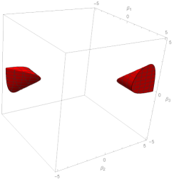
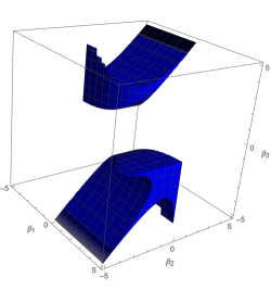
Figure 2. Optimality regions for the saturated design on $(12,23,34)$ on the left and $4$-point designs with $w_{12}=w_{13}=0$ on the right.

5.1.2. The claw graph $K_{1,3}$

We now show that the graph in the middle of Figure 1, sometimes known as a claw, leads to an empty region of optimality. After symmetry reduction it suffices to show that the design $(12,13,14)$ cannot be $D$-optimal. This design would be optimal in the following region given by the three directional derivatives corresponding to the non-edges $(23,24,34)$:

$$\lambda_{23}\leq\frac{\lambda_{12}\lambda_{13}}{\lambda_{12}+\lambda_{13}}\land\lambda_{24}\leq\frac{\lambda_{12}\lambda_{14}}{\lambda_{12}+\lambda_{14}}\land\lambda_{34}\leq\frac{\lambda_{13}\lambda_{14}}{\lambda_{13}+\lambda_{14}}.$$

Plugging in the formulas for the $\lambda_{ij}$ in terms of the $\pi_{i}$ this becomes

$$(\pi_{2}+\pi_{3})\left(\pi_{1}^{2}+\pi_{2}\pi_{3}\right)\leq\pi_{1}(\pi_{2}-\pi_{3})^{2},$$

$$(\pi_{2}+1)\left(\pi_{1}^{2}+\pi_{2}\right)\leq\pi_{1}(\pi_{2}-1)^{2},$$

$$(\pi_{3}+1)\left(\pi_{1}^{2}+\pi_{3}\right)\leq\pi_{1}(\pi_{3}-1)^{2}.$$

Using Mathematica, we find that these conditions are incompatible with $\pi_{1}>0,\pi_{2}>0,\pi_{3}>0$. It would be interesting to find a short certificate for the infeasibility of this system. Such a certificate always exists by the Positivstellensatz from real algebraic geometry (see [BCR13]). This means that if the inequality system has no solution, then one can combine the inequalities to produce an explicit contradiction. There are computational tools to search for such certificates, but our attempts with SOStools [PAV⁺13] were not successful.

5.1.3. Singular designs

Designs corresponding to the rightmost graph in Figure 1 have singular information matrices and can thereby not be $D$-optimal.

Proof of Theorem 12.

Since there are 12 distinct labelings of the path on four vertices, the theorem follows from the computations in Sections 5.1.1–5.1.3. ∎

5.2. Unsaturated Designs

We now examine the designs whose support contains at least four pairs. In this case the weights $w_{ij}$ of an optimal design are not necessarily uniform. Instead we find formulas that express the weights in terms of the parameters. These formulas might look complicated, but they are very symmetric and can easily be handled by computer algebra systems. Our approach is again via Theorem 4: optimality of a design $\xi^{*}$ is equivalent to

(5.2) $$\lambda_{ij}f(i,j)^{T}M(\xi^{*},\beta)^{-1}f(i,j)-3\leq 0,\qquad 1\leq i<j\leq 4.$$

Furthermore, by Corollary 5, there is equality for any pair $i,j$ such that $w_{ij}>0$ in $\xi^{*}$. We distinguish cases according to the size of the support.

5.2.1. Full support

Full support means that all weights of a design are positive. Then all inequalities (5.2) hold with equality and we have a system of 6 equations in the variables $w_{ij},\lambda_{ij}$ for $1\leq i<j\leq 4$. We used Mathematica to solve the system and to express the weights $w_{ij}$ as functions of the intensities $\lambda_{ij}$:

$$w_{ij}=\frac{1}{A}(\lambda_{ik}\lambda_{il}\lambda_{jk}\lambda_{jl}(\lambda_{ij}\lambda_{ik}\lambda_{il}\lambda_{jk}\lambda_{jl}-\lambda_{ij}\lambda_{ik}\lambda_{il}\lambda_{jk}\lambda_{kl}-\lambda_{ij}\lambda_{ik}\lambda_{il}\lambda_{jl}\lambda_{kl}-\lambda_{ij}\lambda_{ik}\lambda_{jk}\lambda_{jl}\lambda_{kl}\\ +\lambda_{ij}\lambda_{ik}\lambda_{jk}\lambda_{kl}^{2}-\lambda_{ij}\lambda_{ik}\lambda_{jl}\lambda_{kl}^{2}-\lambda_{ij}\lambda_{il}\lambda_{jk}\lambda_{jl}\lambda_{kl}-\lambda_{ij}\lambda_{il}\lambda_{jk}\lambda_{kl}^{2}+\lambda_{ij}\lambda_{il}\lambda_{jl}\lambda_{kl}^{2}+2\lambda_{ik}\lambda_{il}\lambda_{jk}\lambda_{jl}\lambda_{kl})),$$

where $(i,j,k,l)$ is any permutation of $(1,2,3,4)$. The term $A$ is the normalization that ensures $\sum_{i<j}w_{ij}=1$.

$$A=3(\lambda_{ij}\lambda_{ik}^{2}\lambda_{il}^{2}\lambda_{jk}^{2}\lambda_{jl}^{2}+\lambda_{ij}\lambda_{ik}\lambda_{il}^{2}\lambda_{jk}\lambda_{jl}^{2}\lambda_{kl}^{2}-\lambda_{ij}\lambda_{ik}\lambda_{il}^{2}\lambda_{jk}^{2}\lambda_{jl}\lambda_{kl}^{2}-\lambda_{ij}^{2}\lambda_{ik}\lambda_{il}^{2}\lambda_{jk}\lambda_{jl}\lambda_{kl}^{2}\\ -\lambda_{ij}\lambda_{ik}\lambda_{il}^{2}\lambda_{jk}^{2}\lambda_{jl}^{2}\lambda_{kl}-\lambda_{ij}\lambda_{ik}^{2}\lambda_{il}^{2}\lambda_{jk}\lambda_{jl}^{2}\lambda_{kl}-\lambda_{ij}\lambda_{ik}^{2}\lambda_{il}^{2}\lambda_{jk}^{2}\lambda_{jl}\lambda_{kl}-\lambda_{ij}^{2}\lambda_{ik}\lambda_{il}^{2}\lambda_{jk}^{2}\lambda_{jl}\lambda_{kl}+\lambda_{ij}^{2}\lambda_{ik}^{2}\lambda_{il}^{2}\lambda_{jk}\lambda_{jl}\lambda_{kl}\\ -\lambda_{ij}\lambda_{ik}^{2}\lambda_{il}\lambda_{jk}\lambda_{jl}^{2}\lambda_{kl}^{2}-\lambda_{ij}^{2}\lambda_{ik}\lambda_{il}\lambda_{jk}\lambda_{jl}^{2}\lambda_{kl}^{2}+\lambda_{ij}\lambda_{ik}^{2}\lambda_{il}\lambda_{jk}^{2}\lambda_{jl}\lambda_{kl}^{2}-\lambda_{ij}^{2}\lambda_{ik}\lambda_{il}\lambda_{jk}^{2}\lambda_{jl}\lambda_{kl}^{2}-\lambda_{ij}^{2}\lambda_{ik}^{2}\lambda_{il}\lambda_{jk}\lambda_{jl}\lambda_{kl}^{2}\\ -\lambda_{ij}\lambda_{ik}^{2}\lambda_{il}\lambda_{jk}^{2}\lambda_{jl}^{2}\lambda_{kl}+\lambda_{ij}^{2}\lambda_{ik}\lambda_{il}\lambda_{jk}^{2}\lambda_{jl}^{2}\lambda_{kl}-\lambda_{ij}^{2}\lambda_{ik}^{2}\lambda_{il}\lambda_{jk}\lambda_{jl}^{2}\lambda_{kl}+\lambda_{ij}^{2}\lambda_{ik}\lambda_{il}^{2}\lambda_{jk}^{2}\lambda_{kl}^{2}+\lambda_{ij}^{2}\lambda_{ik}^{2}\lambda_{il}\lambda_{jl}^{2}\lambda_{kl}^{2}\\ +\lambda_{ij}^{2}\lambda_{ik}^{2}\lambda_{jk}\lambda_{jl}^{2}\lambda_{kl}^{2}+\lambda_{ij}^{2}\lambda_{il}^{2}\lambda_{jk}^{2}\lambda_{jl}\lambda_{kl}^{2}+\lambda_{ik}^{2}\lambda_{il}^{2}\lambda_{jk}^{2}\lambda_{jl}^{2}\lambda_{kl}).$$

This design is locally optimal for some $\beta$ when $w_{ij}>0$ for all $1\leq i<j\leq 4$. Figure 3 shows the optimality region of $6$-point-designs on the left.

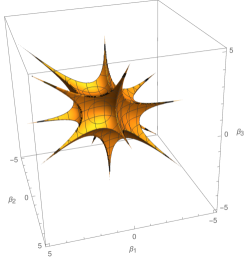
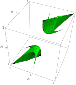
Figure 3. Optimality regions for $6$-point (left) and $5$-point designs with $w_{34}=0$ (right).

Example 13.

A simple example for a design with full support arises when $\beta_{i}=0$ for all $1\leq i\leq 4$. Then $\lambda_{ij}=\frac{1}{4}$ for all $1\leq i<j\leq 4$ and therefore $w_{ij}=\frac{1}{6}$, that is, assigning the same number of repetitions to each comparison, is optimal. Figure 3 and the continuity of the formulas for $w_{ij}$ illustrate that, whenever all $\beta_{i}$ are sufficiently small, an optimal design will assign almost equal number of repetitions to each pair $(i,j)$.

Remark 14.

When working with polynomial equations, Gröbner bases are a powerful tool. The expressions of the $w_{ij}$ in terms of the $\lambda_{ij}$ can also be found using elimination theory. For example, the computer algebra system Macaulay2 [GS] makes this easy.

5.2.2. 5-point designs

We now discuss optimal designs where one weight is zero. There is one orbit under the action of $S_{4}$, that is, a permutation of the alternatives transforms any given five-point design to the one that does not use comparison $(1,2)$. Therefore we discuss the design with $w_{12}=0$ and the remaining weights positive. Then the optimality conditions become

$$w_{13} =\frac{2\lambda_{14}\lambda_{34}\left(\lambda_{14}\lambda_{34}-\lambda_{13}\left(\lambda_{14}+\lambda_{34}\right)\right)}{3\left(\lambda_{13}^{2}\left(\lambda_{14}-\lambda_{34}\right){}^{2}-2\lambda_{13}\lambda_{14}\lambda_{34}\left(\lambda_{14}+\lambda_{34}\right)+\lambda_{14}^{2}\lambda_{34}^{2}\right)},$$

$$w_{14} =\frac{2\lambda_{13}\lambda_{34}\left(\lambda_{13}\left(\lambda_{34}-\lambda_{14}\right)-\lambda_{14}\lambda_{34}\right)}{3\left(\lambda_{13}^{2}\left(\lambda_{14}-\lambda_{34}\right){}^{2}-2\lambda_{13}\lambda_{14}\lambda_{34}\left(\lambda_{14}+\lambda_{34}\right)+\lambda_{14}^{2}\lambda_{34}^{2}\right)},$$

$$w_{23} =\frac{2\lambda_{24}\lambda_{34}\left(\lambda_{24}\lambda_{34}-\lambda_{23}\left(\lambda_{24}+\lambda_{34}\right)\right)}{3\left(\lambda_{23}^{2}\left(\lambda_{24}-\lambda_{34}\right){}^{2}-2\lambda_{23}\lambda_{24}\lambda_{34}\left(\lambda_{24}+\lambda_{34}\right)+\lambda_{24}^{2}\lambda_{34}^{2}\right)},$$

$$w_{24} =\frac{2\lambda_{23}\lambda_{34}\left(\lambda_{23}\left(\lambda_{34}-\lambda_{24}\right)-\lambda_{24}\lambda_{34}\right)}{3\left(\lambda_{23}^{2}\left(\lambda_{24}-\lambda_{34}\right){}^{2}-2\lambda_{23}\lambda_{24}\lambda_{34}\left(\lambda_{24}+\lambda_{34}\right)+\lambda_{24}^{2}\lambda_{34}^{2}\right)},$$

and

$$w_{34}=\frac{1}{B}\Big{(}3\lambda_{13}^{2}\lambda_{14}^{2}\lambda_{23}^{2}\lambda_{24}^{2}-4\lambda_{13}\lambda_{14}\lambda_{23}\lambda_{24}\lambda_{34}^{4}-2\lambda_{13}\lambda_{14}\lambda_{23}^{2}\lambda_{24}^{2}\lambda_{34}^{2}+4\lambda_{13}\lambda_{14}^{2}\lambda_{23}\lambda_{24}^{2}\lambda_{34}^{2}\\ +4\lambda_{13}^{2}\lambda_{14}\lambda_{23}\lambda_{24}^{2}\lambda_{34}^{2}+4\lambda_{13}\lambda_{14}^{2}\lambda_{23}^{2}\lambda_{24}\lambda_{34}^{2}+4\lambda_{13}^{2}\lambda_{14}\lambda_{23}^{2}\lambda_{24}\lambda_{34}^{2}-2\lambda_{13}^{2}\lambda_{14}^{2}\lambda_{23}\lambda_{24}\lambda_{34}^{2}-4\lambda_{13}\lambda_{14}^{2}\lambda_{23}^{2}\lambda_{24}^{2}\lambda_{34}\\ -4\lambda_{13}^{2}\lambda_{14}\lambda_{23}^{2}\lambda_{24}^{2}\lambda_{34}-4\lambda_{13}^{2}\lambda_{14}^{2}\lambda_{23}\lambda_{24}^{2}\lambda_{34}-4\lambda_{13}^{2}\lambda_{14}^{2}\lambda_{23}^{2}\lambda_{24}\lambda_{34}+2\lambda_{13}\lambda_{14}\lambda_{23}^{2}\lambda_{34}^{4}+\lambda_{13}^{2}\lambda_{14}^{2}\lambda_{23}^{2}\lambda_{34}^{2}\\ +2\lambda_{13}\lambda_{14}\lambda_{24}^{2}\lambda_{34}^{4}+\lambda_{13}^{2}\lambda_{14}^{2}\lambda_{24}^{2}\lambda_{34}^{2}+2\lambda_{13}^{2}\lambda_{23}\lambda_{24}\lambda_{34}^{4}+\lambda_{13}^{2}\lambda_{23}^{2}\lambda_{24}^{2}\lambda_{34}^{2}-\lambda_{13}^{2}\lambda_{23}^{2}\lambda_{34}^{4}-\lambda_{13}^{2}\lambda_{24}^{2}\lambda_{34}^{4}\\ +2\lambda_{14}^{2}\lambda_{23}\lambda_{24}\lambda_{34}^{4}+\lambda_{14}^{2}\lambda_{23}^{2}\lambda_{24}^{2}\lambda_{34}^{2}-\lambda_{14}^{2}\lambda_{23}^{2}\lambda_{34}^{4}-\lambda_{14}^{2}\lambda_{24}^{2}\lambda_{34}^{4}\Big{)},\quad\quad\quad$$

with

$$B=3\left(\lambda_{13}^{2}\lambda_{14}^{2}-2\lambda_{13}^{2}\lambda_{14}\lambda_{34}-2\lambda_{13}\lambda_{14}\lambda_{34}^{2}-2\lambda_{13}\lambda_{14}^{2}\lambda_{34}+\lambda_{13}^{2}\lambda_{34}^{2}+\lambda_{14}^{2}\lambda_{34}^{2}\right)\\ \qquad\cdot\left(\lambda_{23}^{2}\lambda_{24}^{2}-2\lambda_{23}^{2}\lambda_{24}\lambda_{34}-2\lambda_{23}\lambda_{24}\lambda_{34}^{2}-2\lambda_{23}\lambda_{24}^{2}\lambda_{34}+\lambda_{23}^{2}\lambda_{34}^{2}+\lambda_{24}^{2}\lambda_{34}^{2}\right).$$

These designs are optimal if the directional derivative in $(1,2)$-direction is smaller than or equal to zero, which is equivalent to

$$\lambda_{12}(\lambda_{13}(\lambda_{14}(\lambda_{23}(\lambda_{24}-\lambda_{34})-\lambda_{24}\lambda_{34})+\lambda_{34}(\lambda_{23}(\lambda_{34}-\lambda_{24})-\lambda_{24}\lambda_{34}))-\lambda_{14}\lambda_{34}(\lambda_{23}(\lambda_{24}+\lambda_{34})-\lambda_{24}\lambda_{34}))\\ \geq-2\lambda_{13}\lambda_{14}\lambda_{23}\lambda_{24}\lambda_{34}.$$

This inequality together with the formulas for the weights and the condition, that all the weights except $w_{12}$ are positive, gives the design region. This region is non-empty. A plot in $\beta$-coordinates is on the right in Figure 3.

5.2.3. 4-point designs

We now discuss designs whose support contain exactly four points. There are $\binom{6}{4}=15$ possibilities for such designs which each have two zero weights, $w_{ij}=w_{kl}=0$. The four-point designs form two orbits under the action of $S_{4}$, distinguished by whether the two non-edges in the graph representation share a vertex or not, that is, whether $|\{i,j,k,l\}|=4$, that is, $i,j,k,l$ are all distinct, or $|\{i,j,k,l\}|=3$, that is, exactly two are equal. In the first case, there are three different design classes. We believe that these designs cannot be $D$-optimal, as the condition $w_{ij}=w_{kl}=0$ with $|\{i,j,k,l\}|=4$ implies that a third weight is zero, which would lead to a saturated design. A proof of this statement eludes us so far. Using Mathematica, it follows from the equivalence theorem that such a design satisfies

(5.3) $$\lambda_{ik}(w_{ik}^{2}-\frac{w_{ik}}{3})=\lambda_{il}(w_{il}^{2}-\frac{w_{il}}{3})=\lambda_{jk}(w_{jk}^{2}-\frac{w_{jk}}{3})=\lambda_{jl}(w_{jl}^{2}-\frac{w_{jl}}{3}),$$

with $0<w_{ik},w_{il},w_{jk},w_{jl}<\frac{1}{3}$ and additionally the inequalities

(5.4) $$\frac{\lambda_{ij}(3(w_{il}+w_{jl})-2)(3(w_{il}+w_{jl})-1)}{\lambda_{jl}w_{jl}(3w_{jl}-1)} \leq 3,$$

(5.5) $$\frac{\lambda_{kl}(3(w_{jk}+w_{jl})-2)(3(w_{jk}+w_{jl})-1)}{\lambda_{jl}w_{jl}(3w_{jl}-1)} \leq 3.$$

Among the solutions of (5.3) there are the saturated designs. If one of the weights equals $1/3$, then (5.3) implies that another weight is zero, i.e. the design is saturated. Since the saturated cases have been dealt with in Theorem 12, we only look for solutions whose weights all lie in the open interval $(0,1/3)$. There are solutions of (5.3) that satisfy this, for example, if the weights and corresponding intensities are equal. In all the cases we examined, the inequalities (5.4) and (5.5) are not satisfied.

Problem 15.

Show that independent of the $\lambda_{ij}$, a simultaneous solution of (5.3), (5.4), and (5.5) is a saturated design.

Finally we analyze the orbit of four-point-designs with $w_{ij}=w_{kl}=0$ with $|\{i,j,k,l\}|=3$. Consider the representative with $w_{12}=w_{13}=0$. Then,

$$w_{14} =\frac{1}{3}$$

$$w_{23} =\frac{2\lambda_{24}\lambda_{34}\left(-\lambda_{23}\lambda_{24}-\lambda_{23}\lambda_{34}+\lambda_{24}\lambda_{34}\right)}{3\left(\lambda_{23}^{2}\lambda_{24}^{2}-2\lambda_{23}^{2}\lambda_{24}\lambda_{34}-2\lambda_{23}\lambda_{24}\lambda_{34}^{2}-2\lambda_{23}\lambda_{24}^{2}\lambda_{34}+\lambda_{23}^{2}\lambda_{34}^{2}+\lambda_{24}^{2}\lambda_{34}^{2}\right)}$$

$$w_{24} =\frac{2\lambda_{23}\lambda_{34}\left(-\lambda_{23}\lambda_{24}+\lambda_{23}\lambda_{34}-\lambda_{24}\lambda_{34}\right)}{3\left(\lambda_{23}^{2}\lambda_{24}^{2}-2\lambda_{23}^{2}\lambda_{24}\lambda_{34}-2\lambda_{23}\lambda_{24}\lambda_{34}^{2}-2\lambda_{23}\lambda_{24}^{2}\lambda_{34}+\lambda_{23}^{2}\lambda_{34}^{2}+\lambda_{24}^{2}\lambda_{34}^{2}\right)}$$

$$w_{34} =\frac{2\lambda_{23}\lambda_{24}\left(\lambda_{24}\lambda_{24}-\lambda_{23}\lambda_{34}-\lambda_{24}\lambda_{34}\right)}{3\left(\lambda_{23}^{2}\lambda_{24}^{2}-2\lambda_{23}^{2}\lambda_{24}\lambda_{34}-2\lambda_{23}\lambda_{24}\lambda_{34}^{2}-2\lambda_{23}\lambda_{24}^{2}\lambda_{34}+\lambda_{23}^{2}\lambda_{34}^{2}+\lambda_{24}^{2}\lambda_{34}^{2}\right)}$$

This design is optimal if the directional derivatives along $(1,2)$ and $(1,3)$ are smaller than 3, so if

$$\frac{3\lambda_{12}(\lambda_{14}+\lambda_{24})}{\lambda_{14}\lambda_{24}}\leq 3~{}\land~{}\frac{3\lambda_{13}(\lambda_{14}+\lambda_{34})}{\lambda_{14}\lambda_{34}}\leq 3.$$

This optimality region for this $4$-point design is visualized in Figure 2 on the right. For each point in the optimality region, the specific weights are computed by the equations above.

Having discussed all cases, it suffices to apply the symmetry to each of these regions and then $\mathbb{R}^{3}$ can be pieced together. Figure 4 gives an idea of this puzzle. Because of continuity, the boundaries between any two regions always belong to the region with fewer design points. Therefore, the yellow amoeba is open, the red regions for saturated designs are closed (by the non-strict inequalities in Theorem 12), and all other regions have both open and closed boundaries.

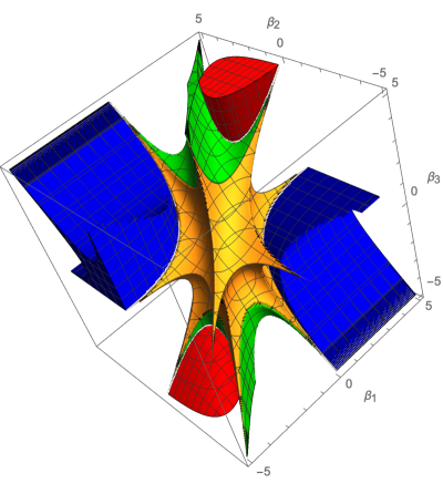
Figure 4. Assembling optimality regions for the Bradley–Terry model.

Remark 16.

Figures 3 and 2 are reminiscent of the amoebas in tropical geometry. It would be interesting to investigate, if the logarithmic algebraic geometry that arises in $\beta$-space from the polynomial constraints in $\lambda$-space offers new insights.

6. Discussion

This paper explains the parameter regions of optimality for experimental design of the Bradley–Terry model, with the strongest results for 4 alternatives. In practical applications this knowledge can be put to use as follows: First, with a screening experiment, initial knowledge of approximate parameters is attained. The initial guess lies in one of the full-dimensional regions illustrated in Figure 4. Depending on which region it is, one can use specific knowledge about the optimal design weights $w_{ij}$. For example, there are explicit polynomial formulas for how the optimal weights depend on the location in parameter space. Section 5 contains explicit such formulas for the case of 4 alternatives.

In the case that a screening experiment reveals parameters in a region where saturated designs are optimal, the solution becomes particularly pleasant: One only needs to assign equal weights to $m-1$ of the pairs. The characterization of regions of optimality of saturated designs is complete, for any number of alternatives (Theorem 11).

We illustrate the effect of choosing the right design by computing the efficiency of the uniform design (assigning equal weights to all pairs) in the case of four alternatives. Consider the line in parameter space that is specified by $2\beta_{2}=\beta_{1}$, $4\beta_{3}=5\beta_{1}$.

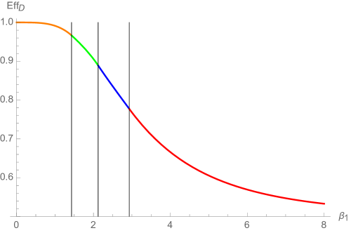
Figure 5. Efficiency of the uniform design along a line in $\beta$-space.

Figure 5 shows the efficiency of the uniform design along that line. At $\beta=(\beta_{1},\beta_{2},\beta_{3})=(0,0,0)$ the uniform design is optimal. As $\beta$ grows, the efficiency decreases. First the weights should be adjusted and starting at approximately $1.4$ a $5$-point design would be optimal. Around $2.1$ a $4$-point design becomes optimal and finally, from $2.9$, a saturated design is optimal. Clearly, working with a uniform design in the case that the support should be smaller is inefficient. In the limit $\beta\to\infty$ the uniform design requires twice as many observations as the optimal saturated design.

We outline some further research directions now. For full support designs, by Corollary 5 the region of optimality is given by the equations

$$\lambda_{ij}f(i,j)^{T}M(\xi^{*},\beta)^{-1}f(i,j)=(m-1)$$

and positivity constraints $\lambda_{ij}>0$. We hope that tools from real algebraic geometry can shed further light on such semi-algebraic sets, especially for designs with full support, as their semi-algebraic sets contain no complicated inequalities.

The Bradley–Terry model considered here is only for the $m$ levels of one attribute and an extension to more attributes is conceivable. The computational challenges of finding optimal designs are formidable and a nice geometry as in the present case is not expected.

In the case of optimality, the equations above express the weights of $\xi$ in terms of the parameters. We conjecture that the equations can be solved in the following sense.

Conjecture 17.

The $\binom{m}{2}$ weights of a fully supported $D$-optimal design are rational functions in the intensities and of numerator degree $\binom{m}{2}+m-1$.

An example of such expressions are the degree 9 equations in Section 5.2.1.

Remark 18.

The solution for the four-dimensional case reveals that the numerator of a weight $w_{ij}$ is a sum of 10 monomials. These monomials can be described combinatorially as follows. For simplicity, let $i=1$ and $j=2$. Then 8 of the 10 monomials are products of the squarefree monomial $\lambda_{12}\lambda_{13}\lambda_{14}\lambda_{23}\lambda_{24}\lambda_{34}$ with monomials of the form $\lambda_{ij}\lambda_{ik}\lambda_{kl}$, where $(ij,ik,kl)$ are edges of the $8$ graphs that are either paths or trees on four vertices and that do not contain the edge $(1,2)$. Furthermore, the monomials that come from a graph with a node of degree $3$ have a positive sign, while the monomials from paths have a negative sign. The remaining two monomials do not show such an easy structure and it remains open, why they are of the form $\lambda_{13}^{2}\lambda_{14}^{2}\lambda_{23}^{2}\lambda_{24}^{2}(\lambda_{12}+2\lambda_{34})$. The complete design is generated by permutations acting on the indices of the numerator described above, while the denominator of the weights is just the sum of all the numerators, that is, a normalization.

From the structure in the case of $4$ alternatives, one can at least partially conjecture the structure of a solution in higher dimensions. In the case of $5$ alternatives, we conjecture that for full support designs the function that expresses $w_{ij}$ in the intensities $\lambda_{ij}$ satisfies the following rules: It is of the form of a polynomial divided by a normalization. The numerator polynomial is of degree $\binom{m}{2}+m-1$ (i.e. 14 for $m=5$) and composed as follows. Start with the monomial $\lambda_{12}\lambda_{13}\cdots\lambda_{m-1,m}$. To construct the weight for the comparison $(1,2)$, multiply it with a square-free product of $m-1$ of the variables $\lambda_{ij}$, where $ij$ is an edge in a spanning tree on $[m]$ which does not contain $(1,2)$. Sum these monomials over all trees that do not contain $(1,2)$. For $n=5$, only 50 out of the 125 trees qualify. In this summation, trees of maximal degree 2 receive a negative sign, the others a positive sign. Additionally, we may have to add monomials of a still unknown structure as in Remark 18 above. We expect a similar structure in the denominator for $5$ alternatives as for four, so that there is a sum of monomials in the denominator that is multiplied by $4$. As there are $125$ trees, this would make $500$ monomials from the tree-structure. This coincides with having $50$ monomials from trees in the numerator, as there are $10$ weights for $5$ alternatives. In comparison, for $4$ alternatives, there are $3\cdot 22=66$ monomials in the denominator, but only $6\cdot 8=48$ come from the described graph structure. The implications of these observations are still unknown.

Acknowledgement

The authors are supported by the Deutsche Forschungsgemeinschaft DFG under grant 314838170, GRK 2297 MathCoRe.

References

• [BCR13] J. Bochnak, M. Coste, and M. Roy. Real algebraic geometry, volume 36. Springer, New York, 2013.
• [BMS04] D. R. Berman, S. C. McLaurin, and D. D. Smith. Ranking whist players. Discrete Math., 283(1-3):15–28, 2004.
• [BT52] R. A. Bradley and M. E. Terry. Rank analysis of incomplete block designs. I. The method of paired comparisons. Biometrika, 39:324–345, 1952.
• [Che53] H. Chernoff. Locally optimal designs for estimating parameters. Ann. Math. Statistics, 24:586–602, 1953.
• [CMP07] T. Callaghan, P. J. Mucha, and M. A. Porter. Random walker ranking for NCAA division I-A football. Amer. Math. Monthly, 114(9):761–777, 2007.
• [DMJ13] J. C. Duchi, L. Mackey, and M. I. Jordan. The asymptotics of ranking algorithms. Ann. Statist., 41(5):2292–2323, 2013.
• [DMP04] H. Dette, V. B Melas, and A. Pepelyshev. Optimal designs for a class of nonlinear regression models. The Annals of Statistics, 32(5):2142–2167, 2004.
• [Fec66] G. T. Fechner. Elemente der Psychophysik (1860). English translation: Howes, D.H., Boring, E.C. (Eds.) and Adler, H.E. (transl.), Elements of Psychophysics. Holt, Rinehart and Winston New York, 1966.
• [Gab00] G. Gabrielsen. Paired comparisons and designed experiments. Food Quality and Preference, 11(1-2):55–61, 2000.
• [GRF03] T. Graves, C. S. Reese, and M. Fitzgerald. Hierarchical models for permutations: analysis of auto racing results. J. Amer. Statist. Assoc., 98(462):282–291, 2003.
• [GS] D. R. Grayson and M. E. Stillman. Macaulay2, a software system for research in algebraic geometry. Available at http://www.math.uiuc.edu/Macaulay2/.
• [GS08] U. Graßhoff and R. Schwabe. Optimal design for the Bradley–Terry paired comparison model. Statistical Methods and Applications, 17(3):275–289, 2008.
• [HT98] T. Hastie and R. Tibshirani. Classification by pairwise coupling. Ann. Statist., 26(2):451–471, 1998.
• [Hun04] D. R. Hunter. MM algorithms for generalized Bradley–Terry models. Ann. Statist., 32(1):384–406, 2004.
• [HYTC20] R. Han, R. Ye, C. Tan, and K. Chen. Asymptotic theory of sparse Bradley–Terry model. Annals of Applied Probability, 30(5):2491–2515, 2020.
• [KKT06] K. Kobayashi, H. Kawasaki, and A. Takemura. Parallel matching for ranking all teams in a tournament. Adv. in Appl. Probab., 38(3):804–826, 2006.
• [KOS16] T. Kahle, K. Oelbermann, and R. Schwabe. Algebraic geometry of Poisson regression. Journal of Algebraic Statistics, 7:29–44, 2016.
• [KRS20] T. Kahle, F. Röttger, and R. Schwabe. Geometrie optimaler Versuchspläne. DMV Mitteilungen, 20(2):71–76, 2020.
• [PAV+13] A. Papachristodoulou, J. Anderson, G. Valmorbida, S. Prajna, P. Seiler, and P. A. Parrilo. SOSTOOLS: Sum of squares optimization toolbox for MATLAB. https://arxiv.org/abs/1310.4716, 2013. Available from http://www.cds.caltech.edu/sostools.
• [Puk06] F. Pukelsheim. Optimal design of experiments. Classics in applied mathematics. Society for Industrial and Applied Mathematics, 2006.
• [RS16] M. Radloff and R. Schwabe. Invariance and equivariance in experimental design for nonlinear models. In J. Kunert, C. H. Müller, and A. C. Atkinson, editors, mODa 11 - Advances in Model-Oriented Design and Analysis Proceedings, pages 217–224. Springer International Publishing, Cham, 2016.
• [Sil80] S.D. Silvey. Optimal design: an introduction to the theory for parameter estimation. Monographs on applied probability and statistics. Chapman and Hall, 1980.
• [SS89] K. R. Shah and B. K. Sinha. Theory of optimal designs, volume 54 of Lecture Notes in Statistics. Springer-Verlag, New York, 1989.
• [SW12] B. Sturmfels and V. Welker. Commutative algebra of statistical ranking. J. Algebra, 361:264–286, 2012.
• [SY99] G. Simons and Y. Yao. Asymptotics when the number of parameters tends to infinity in the Bradley-Terry model for paired comparisons. Ann. Statist., 27(3):1041–1060, 1999.
• [Tor04] B. Torsney. Fitting Bradley Terry models using a multiplicative algorithm. In J. Antoch, editor, COMPSTAT 2004 — Proceedings in Computational Statistics, pages 513–526, Heidelberg, 2004. Physica-Verlag HD.
• [Zer29] E. Zermelo. Die Berechnung der Turnier-Ergebnisse als ein Maximumproblem der Wahrscheinlichkeitsrechnung. Mathematische Zeitschrift, 29:436–460, 1929.