Comments on “Deep Neural Networks with Random Gaussian Weights: A Universal Classification Strategy?”

Abstract

In a recently published paper [1], it is shown that deep neural networks (DNNs) with random Gaussian weights preserve the metric structure of the data, with the property that the distance shrinks more when the angle between the two data points is smaller. We agree that the random projection setup considered in [1] preserves distances with a high probability. But as far as we are concerned, the relation between the angle of the data points and the output distances is quite the opposite, i.e., smaller angles result in a weaker distance shrinkage. This leads us to conclude that Theorem 3 and Figure 5 in [1] are not accurate. Hence the usage of random Gaussian weights in DNNs cannot provide an ability of universal classification or treating in-class and out-of-class data separately. Consequently, the behavior of networks consisting of random Gaussian weights only is not useful to explain how DNNs achieve state-of-art results in a large variety of problems.

I Introduction

Deep neural networks (DNNs) have gained popularity in recent years thanks to their achievements in many applications including computer vision, signal and image processing, speech recognition [2]–[6]. For the purpose of providing insights into remarkable empirical performance of DNNs, the paper [1] focuses on the properties of deep networks with random weights. In particular, it is proved in [1] that the presence of random i.i.d. Gaussian weights provide a distance-preserving embedding for the data points. In the same work, it is also stated (formally in Theorem 3) that DNN layers having random coefficients distort the Euclidean distances “proportionally to the angles between its input points: the smaller the angle at the input, the stronger the shrinkage of the distances.”

Given the fact that the angles between data points belonging to different classes are generally larger than those of the points within the same class [7]–[10], the angle versus distance shrinkage relation asserted in [1] implies “deep neural networks with random weights are universal systems that separates any data (belonging to a low dimensional model) according to the angles between its points”, as stated in [1]. In fact this implication seems to be the main contribution of the paper [1], as evident from the words “a universal classification strategy” being stressed in its title.

The classification ability of DNNs with random weights is emphasized in numerous places throughout the paper [1]. For example, the authors claim in the introduction that “Our theory shows that the addition of ReLU makes the system sensitive to the angles between points. We prove that networks tend to decrease the Euclidean distances between points with a small angle between them (‘same class’), more than the distances between points with large angles between them (‘different classes’)” and “DNN are suitable for models with clearly distinguishable angles between the classes if random weights are used.” In some other sections they have similar statements, such as “It can be observed that the distance between points with a smaller angle between them shrinks more than the distance between points with a larger angle between them. Ideally, we would like this behavior, causing points belonging to the same class to stay closer to each other in the output of the network, compared to points from different classes” and “In general, points within the same class would have small angles within them and points from distinct classes would have larger ones. If this holds for all the points, then random Gaussian weights would be an ideal choice for the network parameters.”

The angle dependence of distance distortion which leads to an ideal classifier is mentioned in the conclusion section of [1] as well, in the following lines: “While preserving the structure of the initial metric is important, it is vital to have the ability to distort some of the distances in order to deform the data in a way that the Euclidean distances represent more faithfully the similarity we would like to have between points from the same class. We proved that such an ability is inherent to the DNN architecture: the Euclidean distances of the input data are distorted throughout the networks based on the angles between the data points. Our results lead to the conclusion that DNNs are universal classifiers for data based on the angles of the principal axis between the classes in the data.”

It is also worthwhile to mention the papers citing [1]. Most of the papers cite [1] in an undetailed fashion as one of the papers providing some theoretical analysis for DNNs [11]–[13] or as a study showing us the distance-preserving aspect of random DNN weights [13, 14]. But still some remarks on the classification property associated with random weights, similarly to the ones made by [1], are encountered in some of the papers citing [1], such as “According to their observation, random filters are in fact a good choice if training data are initially well-separated” in [15], “Deep networks with random weights are a universal system that separates any data (belonging to a low-dimensional model) according to the angles between the data points, where the general assumption is that there are large angles between different classes” in [16], “Giryes et al. (2015) proved that under random Gaussian weights, deep neural networks are distance-preserving mappings with a special treatment for intra- and inter-class data” in [17], “Randomness of features has been used with great success as a mean of reducing the computational complexity of neural networks while achieving comparable performance as with fully learnt networks” in [18], “The authors demonstrate that this form of nonlinear random projection performs a class-aware embedding where the embedding places objects of the same class closer to one another after the projection compared to objects of different classes” and “such embeddings tend to decrease the Euclidean distances between points with a small angle between them (‘same class’) more than the distances between points with large angles between them (‘different classes’)” in [19], and “The model structure of the RVFL is so simple, why does the RVFL work well for most tasks? Giryes et. al. give a possible theoretical explanation for this open problem.” (here RVFL is the abbreviation for random vector functional link) in [20].

In this work, we argue that the claims quoted above and made by [1] along with some of the papers citing it in regards to the universal classification or class-aware embedding require reconsideration by disproving Theorem 3 (more precisely Eq. (4)) in [1]. For that purpose, we consider the problem setup of this theorem and calculate the expectation of the squared norm term appearing in the theorem statement. This would be the subject of Section II, where we also show for a single layer of a randomly weighted DNN that smaller angle values between the input pairs cause a larger output Euclidean distance to input Euclidean distance ratio, contrary to what is claimed by [1]. We briefly discuss Theorem 4 and derive the revised form of Corollary 5 in [1], in Section III. Lastly, we discuss the consequences of our derivations in conjunction with the simulation results presented by [1] in Section IV.

II Problem Definition and The Revised Distance Distortion Result

The effect of a single layer of DNN on the Euclidean distances is considered in [1], with $\rho$ being the rectified linear unit (ReLU) activation function, ${\mathbf{M}}$ being the linear operator, and $\rho({\mathbf{M}}\cdot)$ accounting for the transformation applied at a single layer. Denoting the Euclidean ball of radius $r$ by ${\mathbb{B}}_{r}^{n}\subset{\mathbb{R}}^{n}$, the authors of [1] prove the following theorem.

Theorem (Theorem 3 in [1]).

Let $K\subset{\mathbb{B}}_{1}^{n}$ be the manifold of the data in the input layer. If $\sqrt{m}{\mathbf{M}}\in{\mathbb{R}}^{m\times n}$ is a random matrix with i.i.d. normally distributed entries and $m\geq C\delta^{-4}\omega(K)^{4}$ (here $\omega(K)$ is the Gaussian mean width defined as $\omega(K)\triangleq{\mathbb{E}}[\sup_{{\mathbf{x}},{\mathbf{y}}\in K}\langle{\mathbf{g}},{\mathbf{x}}-{\mathbf{y}}\rangle]$), then with a high probability (of the form $1-\exp(-O(\delta^{2}))$) the inequality given by

$$\Bigg{|}\|\rho(\mathbf{Mx})-\rho(\mathbf{My})\|_{2}^{2}$$

$$\quad-\left(\frac{1}{2}\|{\mathbf{x}}-{\mathbf{y}}\|_{2}^{2}+\|{\mathbf{x}}\|_{2}\|{\mathbf{y}}\|_{2}\psi({\mathbf{x}},{\mathbf{y}})\right)\Bigg{|}\leq\delta$$ (1)

holds, where

$$\psi({\mathbf{x}},{\mathbf{y}})=\frac{1}{\pi}\left(\sin\angle({\mathbf{x}},{\mathbf{y}})-\angle({\mathbf{x}},{\mathbf{y}})\cos\angle({\mathbf{x}},{\mathbf{y}})\right)$$ (2)

with $0\leq\angle({\mathbf{x}},{\mathbf{y}})\triangleq\cos^{-1}\left(\frac{{\mathbf{x}}^{T}{\mathbf{y}}}{\|{\mathbf{x}}\|_{2}\|{\mathbf{y}}\|_{2}}\right)\leq\pi.$

The proof of Theorem 3 in [1] relies on some concentration inequality for Lipschitz–continuous functions of Gaussian random variables and Bernstein’s inequality, together with the observation that

$${\mathbb{E}}\|\rho(\mathbf{Mx})-\rho(\mathbf{My})\|_{2}^{2}=\frac{1}{2}\|{\mathbf{x}}-{\mathbf{y}}\|_{2}^{2}+\|{\mathbf{x}}\|_{2}\|{\mathbf{y}}\|_{2}\psi({\mathbf{x}},{\mathbf{y}}),$$ (3)

see Eq. (22) in [1]. The function $\psi(\theta)=\frac{1}{\pi}(\sin\theta-\theta\cos\theta)$ is increasing on the interval $[0,\pi]$, and consequently it follows from (1) that the smaller the angle between ${\mathbf{x}}$ and ${\mathbf{y}}$, the smaller the output distance turns out to be. This behavior of a single layer of DNN with random weights is also summarized in Fig. 5 of [1], where it is illustrated that two classes with distinguishable angles can be separated using such networks.

In the rest of this section, we evaluate the expression ${\mathbb{E}}\|\rho(\mathbf{Mx})-\rho(\mathbf{My})\|_{2}^{2}$, and show that (3) (and thus Theorem 3 in [1]) is not true. For that purpose, we first remind the reader Eq. (18) and Eq. (19) in [1]:

$$\|\rho(\mathbf{Mx})-\rho(\mathbf{My})\|_{2}^{2} =\sum_{i=1}^{m}\left(\rho({\mathbf{m}}_{i}^{T}{\mathbf{x}})-\rho({\mathbf{m}}_{i}^{T}{\mathbf{y}})\right)^{2}$$ (4)

$${\mathbb{E}}\left(\rho({\mathbf{m}}_{i}^{T}{\mathbf{x}})-\rho({\mathbf{m}}_{i}^{T}{\mathbf{y}})\right)^{2} ={\mathbb{E}}\left(\rho({\mathbf{m}}_{i}^{T}{\mathbf{x}})\right)^{2}+{\mathbb{E}}\left(\rho({\mathbf{m}}_{i}^{T}{\mathbf{y}})\right)^{2}$$

$$\quad-2\,{\mathbb{E}}\left[\rho({\mathbf{m}}_{i}^{T}{\mathbf{x}})\rho({\mathbf{m}}_{i}^{T}{\mathbf{y}})\right].$$ (5)

The terms ${\mathbb{E}}\left(\rho({\mathbf{m}}_{i}^{T}{\mathbf{x}})\right)^{2}$ and ${\mathbb{E}}\left(\rho({\mathbf{m}}_{i}^{T}{\mathbf{y}})\right)^{2}$ appearing in (5) can be easily computed from the symmetry of Gaussian distribution as

$${\mathbb{E}}\left(\rho({\mathbf{m}}_{i}^{T}{\mathbf{x}})\right)^{2} =\frac{1}{2}\,{\mathbb{E}}\left({\mathbf{m}}_{i}^{T}{\mathbf{x}}\right)^{2}$$

$$=\frac{1}{2}\sum_{k=1}^{n}{\mathbb{E}}({\mathbf{m}}_{i}(k))^{2}({\mathbf{x}}(k))^{2}$$

$$=\frac{1}{2m}\|{\mathbf{x}}\|_{2}^{2}$$ (6)

$${\mathbb{E}}\left(\rho({\mathbf{m}}_{i}^{T}{\mathbf{y}})\right)^{2} =\frac{1}{2m}\|{\mathbf{y}}\|_{2}^{2},$$ (7)

consistently with Eq. (20) in [1], where $k$ in brackets denote the $k^{\text{th}}$ component of the corresponding vector.

To evaluate the expression ${\mathbb{E}}[\rho({\mathbf{m}}_{i}^{T}{\mathbf{x}})\rho({\mathbf{m}}_{i}^{T}{\mathbf{y}})]$ in (5), we make use of the fact that the projection ${\mathbf{m}}_{i}^{p}$ of the Gaussian random vector ${\mathbf{m}}_{i}$ to the plane spanned by ${\mathbf{x}}$ and ${\mathbf{y}}$ is another Gaussian with expected squared norm $2/m$, as long as ${\mathbf{x}}\neq{\mathbf{y}}.$ If the angle between ${\mathbf{m}}_{i}^{p}$ and ${\mathbf{x}}$ is $\boldsymbol{\theta}\in[-\pi,\pi]$, then the angle between ${\mathbf{m}}_{i}^{p}$ and ${\mathbf{y}}$ can be taken as $\boldsymbol{\theta}+\angle({\mathbf{x}},{\mathbf{y}})$ without loss of generality (please see Fig. 1).

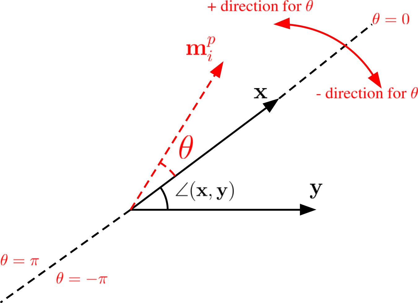
Figure 1: The angle between ${\mathbf{m}}_{i}^{p}$ and ${\mathbf{y}}$ equals to $\boldsymbol{\theta}+\angle({\mathbf{x}},{\mathbf{y}})$, $\boldsymbol{\theta}$ takes values between $-\pi$ and $\pi.$

In this case we would have

$${\mathbf{m}}_{i}^{T}{\mathbf{x}}=({\mathbf{m}}_{i}^{p})^{T}{\mathbf{x}}=\|{\mathbf{m}}_{i}^{p}\|_{2}\|{\mathbf{x}}\|_{2}\cos\boldsymbol{\theta}$$

$${\mathbf{m}}_{i}^{T}{\mathbf{y}}=({\mathbf{m}}_{i}^{p})^{T}{\mathbf{y}}=\|{\mathbf{m}}_{i}^{p}\|_{2}\|{\mathbf{y}}\|_{2}\cos(\boldsymbol{\theta}+\angle({\mathbf{x}},{\mathbf{y}}))$$

The product $\rho({\mathbf{m}}_{i}^{T}{\mathbf{x}})\rho({\mathbf{m}}_{i}^{T}{\mathbf{y}})$ is non-zero only when

$$\cos\boldsymbol{\theta}>0,\quad\cos(\boldsymbol{\theta}+\angle({\mathbf{x}},{\mathbf{y}}))>0,\,\,\boldsymbol{\theta}\in[-\pi,\pi]$$ (8)

So the inequality $\cos(\boldsymbol{\theta}+\angle({\mathbf{x}},{\mathbf{y}}))>0$ needs to be satisfied under the constraint $\boldsymbol{\theta}\in(-\pi/2,\pi/2).$ Note that $0\leq\angle({\mathbf{x}},{\mathbf{y}})\leq\pi$ by definition, meaning that (8) implies $\boldsymbol{\theta}+\angle({\mathbf{x}},{\mathbf{y}})\in(-\pi/2,3\pi/2).$ But cosine function is non-positive in the interval $[\pi/2,3\pi/2].$ Thus the set of conditions (8) is satisfied if and only if

$$-\pi/2<\boldsymbol{\theta}<\pi/2,\quad-\pi/2<\boldsymbol{\theta}+\angle({\mathbf{x}},{\mathbf{y}})<\pi/2,$$

which is equivalent to the single inequality given by

$$-\pi/2<\boldsymbol{\theta}<\pi/2-\angle({\mathbf{x}},{\mathbf{y}}).$$

Thus we can express the expectation ${\mathbb{E}}[\rho({\mathbf{m}}_{i}^{T}{\mathbf{x}})\rho({\mathbf{m}}_{i}^{T}{\mathbf{y}})]$ as

$$\color[rgb]{0,0,0}{{\mathbb{E}}[\rho({\mathbf{m}}_{i}^{T}{\mathbf{x}})\rho({\mathbf{m}}_{i}^{T}{\mathbf{y}})]=\|{\mathbf{x}}\|_{2}\|{\mathbf{y}}\|_{2}{\mathbb{E}}\|{\mathbf{m}}_{i}^{p}\|^{2}_{2}}$$

$$\,\color[rgb]{0,0,0}{\cdot{\mathbb{E}}\left[\cos\boldsymbol{\theta}\,\cos(\boldsymbol{\theta}+\angle({\mathbf{x}},{\mathbf{y}}){\mathbbm{1}}(-\pi/2<\boldsymbol{\theta}<\pi/2-\angle({\mathbf{x}},{\mathbf{y}}))\right]}$$

$$\color[rgb]{0,0,0}{=\frac{2\|{\mathbf{x}}\|_{2}\|{\mathbf{y}}\|_{2}}{m}\int_{-\pi/2}^{\pi/2-\angle({\mathbf{x}},{\mathbf{y}})}\cos\boldsymbol{\theta}\,\cos(\boldsymbol{\theta}+\angle({\mathbf{x}},{\mathbf{y}}))\,\frac{d\boldsymbol{\theta}}{2\pi}}$$

$$=\frac{\|{\mathbf{x}}\|_{2}\|{\mathbf{y}}\|_{2}}{m\pi}$$

$$\quad\cdot\int_{-\pi/2}^{\pi/2-\angle({\mathbf{x}},{\mathbf{y}})}\sin\left(\boldsymbol{\theta}+\frac{\pi}{2}\right)\sin\left(\boldsymbol{\theta}+\frac{\pi}{2}+\angle({\mathbf{x}},{\mathbf{y}})\right)\,d\boldsymbol{\theta}$$

$$=\frac{\|{\mathbf{x}}\|_{2}\|{\mathbf{y}}\|_{2}}{m\pi}\int_{0}^{\pi-\angle({\mathbf{x}},{\mathbf{y}})}\sin\boldsymbol{\theta}\,\sin(\boldsymbol{\theta}+\angle({\mathbf{x}},{\mathbf{y}}))\,d\boldsymbol{\theta}.$$ (9)

Inserting the equations (6)–(9) in (5), we get

$${\mathbb{E}}\left(\rho({\mathbf{m}}_{i}^{T}{\mathbf{x}})-\rho({\mathbf{m}}_{i}^{T}{\mathbf{y}})\right)^{2}=\frac{1}{m}\bigg{(}\frac{\|{\mathbf{x}}\|_{2}^{2}}{2}+\frac{\|{\mathbf{y}}\|_{2}^{2}}{2}$$

$$\quad-2\frac{\|{\mathbf{x}}\|_{2}\|{\mathbf{y}}\|_{2}}{\pi}\int_{0}^{\pi-\angle({\mathbf{x}},{\mathbf{y}})}\sin\boldsymbol{\theta}\,\sin(\boldsymbol{\theta}+\angle({\mathbf{x}},{\mathbf{y}}))\,d\boldsymbol{\theta}\bigg{)},$$

from which

$${\mathbb{E}}\|\rho(\mathbf{Mx})-\rho(\mathbf{My})\|_{2}^{2}=\frac{\|{\mathbf{x}}\|_{2}^{2}}{2}+\frac{\|{\mathbf{y}}\|_{2}^{2}}{2}$$

$$\quad-2\frac{\|{\mathbf{x}}\|_{2}\|{\mathbf{y}}\|_{2}}{\pi}\int_{0}^{\pi-\angle({\mathbf{x}},{\mathbf{y}})}\sin\boldsymbol{\theta}\,\sin(\boldsymbol{\theta}+\angle({\mathbf{x}},{\mathbf{y}}))\,d\boldsymbol{\theta}\vspace{-.1in}$$ (10)

follows trivially due to (4). Comparing (10) with eq. (11) in [1], we observe there is a missing multiplicative factor of $-2$ for the coefficient of the integral term of eq. (11) in [1]. To evaluate the integral, we write

$$\int_{0}^{\pi-\angle({\mathbf{x}},{\mathbf{y}})}\sin\boldsymbol{\theta}\,\sin(\boldsymbol{\theta}+\angle({\mathbf{x}},{\mathbf{y}}))\,d\boldsymbol{\theta}$$

$$=\int_{0}^{\pi-\angle({\mathbf{x}},{\mathbf{y}})}\left[\frac{\cos\angle({\mathbf{x}},{\mathbf{y}})-\cos(2\boldsymbol{\theta}+\angle({\mathbf{x}},{\mathbf{y}}))}{2}\right]\,d\boldsymbol{\theta}$$

$$\quad=-\frac{\sin(2\boldsymbol{\theta}+\angle({\mathbf{x}},{\mathbf{y}}))}{4}\bigg{|}_{0}^{\pi-\angle({\mathbf{x}},{\mathbf{y}})}\!\!\!\!\!\!+\frac{\pi-\angle({\mathbf{x}},{\mathbf{y}})}{2}\cos\angle({\mathbf{x}},{\mathbf{y}})$$

$$\quad=\frac{\sin\angle({\mathbf{x}},{\mathbf{y}})}{2}+\frac{\pi-\angle({\mathbf{x}},{\mathbf{y}})}{2}\cos\angle({\mathbf{x}},{\mathbf{y}})$$

$$\quad=\frac{\pi}{2}\cos\angle({\mathbf{x}},{\mathbf{y}})+\frac{1}{2}\left(\sin\angle({\mathbf{x}},{\mathbf{y}})-\angle({\mathbf{x}},{\mathbf{y}})\cos\angle({\mathbf{x}},{\mathbf{y}})\right).$$ (11)

Note that the right hand side of (11) is one half of the term in brackets appearing in eq. (21) of [1], so they are not equal. Combining (11) with (10), we obtain

$${\mathbb{E}}\|\rho(\mathbf{Mx})-\rho(\mathbf{My})\|_{2}^{2}$$

$$\,\,=\frac{\|{\mathbf{x}}\|_{2}^{2}}{2}+\frac{\|{\mathbf{y}}\|_{2}^{2}}{2}-\|{\mathbf{x}}\|_{2}\|{\mathbf{y}}\|_{2}\cos\angle({\mathbf{x}},{\mathbf{y}})$$

$$\quad-\frac{\|{\mathbf{x}}\|_{2}\|{\mathbf{y}}\|_{2}}{\pi}\left(\sin\angle({\mathbf{x}},{\mathbf{y}})-\angle({\mathbf{x}},{\mathbf{y}})\cos\angle({\mathbf{x}},{\mathbf{y}})\right)$$

$$\,\,=\frac{\|{\mathbf{x}}\|_{2}^{2}}{2}+\frac{\|{\mathbf{y}}\|_{2}^{2}}{2}-{\mathbf{x}}^{T}{\mathbf{y}}-\|{\mathbf{x}}\|_{2}\|{\mathbf{y}}\|_{2}\psi({\mathbf{x}},{\mathbf{y}})$$ (12)

$$\,\,=\frac{1}{2}\|{\mathbf{x}}-{\mathbf{y}}\|_{2}^{2}-\|{\mathbf{x}}\|_{2}\|{\mathbf{y}}\|_{2}\psi({\mathbf{x}},{\mathbf{y}})$$ (13)

where we substitute $\psi({\mathbf{x}},{\mathbf{y}})$ of (2) in (12).

When we compare (13) with (3) (or with Eq. (22) in [1]), we see there is a plus–minus difference associated with the angle–dependent term $\|{\mathbf{x}}\|_{2}\|{\mathbf{y}}\|_{2}\psi({\mathbf{x}},{\mathbf{y}}).$ This difference changes the conclusion of the derivation fundamentally, i.e., it turns out the distance shrinkage that the operator $\rho({\mathbf{M}}\cdot)$ induces is greater when the angle between the points is greater. Therefore the way a DNN with random weights discriminates angles does not make the classification task any easier at all, meaning that the classification behavior illustrated by Fig. 5 in [1] cannot be valid.

Before closing this section, we would like to inform the reader that the usage of Bernstein’s inequality and the Gaussian concentration bound in Appendix A of [1] are correct to the best of our understanding. Hence following the same lines of reasoning as presented there, it is possible to prove the following.

Theorem 1.

Let $K\subset{\mathbb{B}}_{1}^{n}$ be the manifold of the data in the input layer. If $\sqrt{m}{\mathbf{M}}\in{\mathbb{R}}^{m\times n}$ is a random matrix with i.i.d. normally distributed entries and if $m$ is sufficiently large (as defined in [1]), then with a high probability (of the form $1-\exp(-O(\delta^{2}))$)

$$\Bigg{|}\|\rho(\mathbf{Mx})-\rho(\mathbf{My})\|_{2}^{2}$$

$$\quad-\left(\frac{1}{2}\|{\mathbf{x}}-{\mathbf{y}}\|_{2}^{2}-\|{\mathbf{x}}\|_{2}\|{\mathbf{y}}\|_{2}\psi({\mathbf{x}},{\mathbf{y}})\right)\Bigg{|}\leq\delta.$$ (14)

Theorem 1 further corroborates our claim that DNNs with random weights cannot treat in–class and out–of–class data in an ideal way. Equation (14) implies inter–class points and intra–class points are treated in an exactly opposite manner with high probability.

III Angle Distortion and Distance Shrinkage Bound

The angular distance result for a single layer of randomly weighted DNN is provided by Theorem 4 in [1] as follows.

Theorem (Theorem 4 in [1]).

Under the same conditions of Theorem 3 in [1] and $K\subset{\mathbb{B}}_{1}^{n}\backslash{\mathbb{B}}_{\beta}^{n}$, where $\delta\ll\beta^{2}<1$, with high probability

$$\bigg{|}\cos\angle(\rho({\mathbf{M}}{\mathbf{x}}),\rho({\mathbf{M}}{\mathbf{y}}))-(\cos\angle({\mathbf{x}},{\mathbf{y}}) +\psi({\mathbf{x}},{\mathbf{y}}))\bigg{|}$$

$$\quad\leq\frac{15\delta}{\beta^{2}-2\delta}.$$ (15)

This theorem is proved in Appendix B of [1]. The proof relies on the inequality

$$\bigg{|}\frac{1}{2}\|\rho({\mathbf{M}}{\mathbf{x}})\|_{2}^{2}+\frac{1}{2}\|\rho({\mathbf{M}}{\mathbf{y}})\|_{2}^{2}-\frac{1}{4}\|{\mathbf{x}}\|_{2}^{2}-\frac{1}{4}\|{\mathbf{y}}\|_{2}^{2}$$

$$\quad-\bigg{(}\rho({\mathbf{M}}{\mathbf{x}})^{T}\rho({\mathbf{M}}{\mathbf{y}})-\frac{\|{\mathbf{x}}\|_{2}\|{\mathbf{y}}\|_{2}}{2}\cos\angle({\mathbf{x}},{\mathbf{y}})$$

$$\quad-\frac{\|{\mathbf{x}}\|\|{\mathbf{y}}\|}{2\pi}(\sin\angle({\mathbf{x}},{\mathbf{y}})-\angle({\mathbf{x}},{\mathbf{y}})\cos\angle({\mathbf{x}},{\mathbf{y}}))\bigg{)}\bigg{|}\leq\frac{\delta}{2}$$ (16)

which is given by Eq. (30) in [1], where the authors also state that this inequality is equivalent to Eq. (4) in [1] ((1) in this work).

Observing that both $\cos\angle({\mathbf{x}},{\mathbf{y}}))$ and $(\sin\angle({\mathbf{x}},{\mathbf{y}})-\angle({\mathbf{x}},{\mathbf{y}})\cos\angle({\mathbf{x}},{\mathbf{y}}))$ terms have the same sign in (16), it can be seen easily that (16) (Eq. (30) in [1]) is not consistent with (1) (Eq. (4) in [1]), i.e., this part of Appendix B in [1] seems to be inaccurate. In fact, it is relatively straightforward to show that (16) is equivalent to (14). Hence we conclude (16) is correct even if its justification in Appendix B of [1] is not.

Consequently Theorem 4 in [1] accurately describes the angular distance behavior for a single DNN layer with random weights. Note that the experimental results with ImageNet deep network demonstrated by Fig. 4 in [1] is in full accordance with Theorem 4, as explained in [1].

Now we turn our attention to the bounds on the shrinkage of distances given by Corollary 5 in [1].

Corollary (Corollary 5 in [1]).

Under the same conditions of Theorem 3 in [1], with high probability(depending on $\delta$ as in Theorem 3 in [1])

$$\frac{1}{2}\|{\mathbf{x}}-{\mathbf{y}}\|_{2}^{2}-\delta\leq\|\rho({\mathbf{M}}{\mathbf{x}})-\rho({\mathbf{M}}{\mathbf{y}})\|_{2}^{2}\leq\|{\mathbf{x}}-{\mathbf{y}}\|_{2}^{2}+\delta$$ (17)

It follows from our Theorem 1 that (17) needs to be corrected, and its corrected version is given below, along with the proof. We conclude from Corollary 18 that the local structure of the data points is preserved with high probability by the transform $\rho({\mathbf{M}}\cdot).$

Corollary 2.

Under the same conditions of Theorem 3 in [1], with high probability(of the form $1-\exp(-O(\delta^{2}))$)

$$\frac{1}{4}\|{\mathbf{x}}-{\mathbf{y}}\|_{2}^{2}-\delta\leq\|\rho({\mathbf{M}}{\mathbf{x}})-\rho({\mathbf{M}}{\mathbf{y}})\|_{2}^{2}\leq\frac{1}{2}\|{\mathbf{x}}-{\mathbf{y}}\|_{2}^{2}+\delta$$ (18)

Proof.

Equation (14) implies it is sufficient to prove

$$\frac{1}{4}\|{\mathbf{x}}-{\mathbf{y}}\|_{2}^{2}\leq\frac{1}{2}\|{\mathbf{x}}-{\mathbf{y}}\|_{2}^{2}-\|{\mathbf{x}}\|_{2}\|{\mathbf{y}}\|_{2}\psi({\mathbf{x}},{\mathbf{y}})\leq\frac{1}{2}\|{\mathbf{x}}-{\mathbf{y}}\|_{2}^{2}$$ (19)

Since $\psi({\mathbf{x}},{\mathbf{y}})$ is non-negative, it is trivial to see

$$\frac{1}{2}\|{\mathbf{x}}-{\mathbf{y}}\|_{2}^{2}-\|{\mathbf{x}}\|_{2}\|{\mathbf{y}}\|_{2}\psi({\mathbf{x}},{\mathbf{y}})\leq\frac{1}{2}\|{\mathbf{x}}-{\mathbf{y}}\|_{2}^{2}.$$ (20)

To prove the lower bound in (19), we write

$$\frac{1}{2}\|{\mathbf{x}}-{\mathbf{y}}\|_{2}^{2}-\|{\mathbf{x}}\|_{2}\|{\mathbf{y}}\|_{2}\psi({\mathbf{x}},{\mathbf{y}})$$

$$\,\,=\frac{1}{2}\|{\mathbf{x}}-{\mathbf{y}}\|_{2}^{2}$$

$$\quad-\frac{\|{\mathbf{x}}\|_{2}\|{\mathbf{y}}\|_{2}}{\pi}(\sin\angle({\mathbf{x}},{\mathbf{y}})-\angle({\mathbf{x}},{\mathbf{y}})\cos\angle({\mathbf{x}},{\mathbf{y}}))$$

$$\,\,\geq\frac{1}{2}\|{\mathbf{x}}-{\mathbf{y}}\|_{2}^{2}+\left(\frac{\cos\angle({\mathbf{x}},{\mathbf{y}})-1}{2}\right)\|{\mathbf{x}}\|_{2}\|{\mathbf{y}}\|_{2}$$ (21)

$$\,\,=\frac{{\mathbf{x}}^{T}{\mathbf{x}}}{2}+\frac{{\mathbf{y}}^{T}{\mathbf{y}}}{2}-\frac{{\mathbf{x}}^{T}{\mathbf{y}}}{2}-\frac{\|{\mathbf{x}}\|_{2}\|{\mathbf{y}}\|_{2}}{2}$$

$$\,\,=\frac{1}{4}\|{\mathbf{x}}-{\mathbf{y}}\|_{2}^{2}+\frac{1}{4}(\|{\mathbf{x}}\|_{2}-\|{\mathbf{y}}\|_{2})^{2}$$

$$\,\,\geq\frac{1}{4}\|{\mathbf{x}}-{\mathbf{y}}\|_{2}^{2}$$ (22)

where we have (21) because of $\psi({\mathbf{x}},{\mathbf{y}})$ being a convex function of $\cos\angle({\mathbf{x}},{\mathbf{y}}).$ (Note that $\psi({\mathbf{x}},{\mathbf{y}})=\frac{1}{\pi}(\sqrt{1-\cos^{2}\angle({\mathbf{x}},{\mathbf{y}})}-\cos^{-1}(\cos\angle({\mathbf{x}},{\mathbf{y}}))\cos\angle({\mathbf{x}},{\mathbf{y}}))$ and the second derivative of $f(t)=\frac{1}{\pi}(\sqrt{1-t^{2}}-t\cos^{-1}(t))$ is $f^{\prime\prime}(t)=\frac{1}{\pi\sqrt{1-t^{2}}}>0.$) ∎

IV Discussions and Conclusions

For a single DNN layer with random Gaussian weights, we have seen in Theorem 1 that the separation of classes with distinguishable angles becomes more difficult, and proved in Corollary 18 that the metric structure of the data manifold is not altered. It is possible to extend those results along with the angular distortion result given by Theorem 4 in [1] to the entire network by resorting to the covering number arguments of Section IV (particularly Theorem 6) in [1].

In fact, our findings in regard to the angular separation inability of randomly weighted DNNs are supported by the experimental results in Section VI of [1]. We see from Figs. 6(a)–(b) and Figs. 7(a)–(b) in [1] that closest inter–class Euclidean distances decrease(the blue curve in Fig.6(a) is biased below 1) and farthest intra–class Euclidean distances increase for CIFAR–10 dataset(the blue curve in Fig.6(b) is biased above 1). This behavior is in strict contrast with the performance of the trained networks and with what a “universal classifier” that Theorem 3 in [1] predicts is supposed to do. Theorem 1 we present here explains this discrepancy very well. Similar comments apply to Figs. 10(a)–(b) and Figs. 11(a)–(b) in [1], where we observe for ImageNet dataset that closest inter-class Euclidean distances do shrink but farthest intra-class Euclidean distances do not.

The experiments considered by [1] is consistent with the existence of distance lower and upper bounds we state in Corollary 18 as well. For a randomly weighted DNN, Figs. 8(a)–(b), Figs. 9(a)–(b) and Figs. 12(a)–(b), Figs. 13(a)–(b) in [1] demonstrate that there is no difference between inter-class and intra-class points in terms of the distance ratios for CIFAR–10 dataset and ImageNet dataset, respectively. Those results confirm Corollary 18 since the distance bounds in this corollary are valid for both intra-class and inter-class points.

We know that a complete and profound theoretical explanation for the practical performance of DNNs is still unavailable. Analysis and properties of DNNs involving randomness or random weights are considered by a significant number of papers including [21]–[27]. We hope this work will shed some light on random matrix theory based approaches and initiate some rethinking, perhaps similarly to the way [28] contributed to the literature on the generalization subject.

References

- [1] R. Giryes, G. Sapiro, and A. M. Bronstein, “Deep Neural Networks with Random Gaussian Weights: A Universal Classification Strategy?,” IEEE Trans. Signal Process., vol. 64, no. 13, pp. 3444–3457, 2016.
- [2] A. Krizhevsky, I. Sutskever, and G. E. Hinton, “Imagenet classification with deep convolutional neural networks,” Proc. Int. Conf. Adv. Neural Inf. Process. Syst., 2012, pp. 1097–1105.
- [3] G. Hinton, L. Deng, D. Yu, G. E. Dahl, A. R. Mohamed, N. Jaitly, A. Senior, V. Vanhoucke, P. Nguyen, T. N. Sainath, and B. Kingsbury, “Deep neural networks for acoustic modeling in speech recognition: The shared views of four research groups,” IEEE Signal Process. Mag., vol. 29, no. 6, pp. 82–97, 2012.
- [4] C. Farabet, C. Couprie, L. Najman, and Y. LeCun, “Learning hierarchical features for scene labeling,” IEEE Trans. Pattern Anal. Mach. Intell., vol. 35, no. 8, pp. 1915–1929, 2013.
- [5] C. Dong, C. C. Loy, K. He, and X. Tang, “Image super-resolution using deep convolutional networks,” IEEE Trans. Pattern Anal. Mach. Intell., vol. 38, no. 2, pp. 295–307, 2016.
- [6] C. Szegedy, S. Ioffe, V. Vanhoucke, and A. A. Alemi, “Inception-v4, Inception-ResNet and the impact of residual connections on learning,” Proc. AAAI Conf. on Artif. Intell., vol. 4, 2017, pp. 4278–4284.
- [7] O. Yamaguchi, K. Fukui, and K. Maeda, “Face recognition using temporal image sequence,” Proc. IEEE Int. Conf. Autom. Face Gesture Recogn., pp. 318–323, 1998.
- [8] L. Wolf and A. Shashua, “Learning over sets using kernel principal angles,” J. Mach. Learn. Res., vol. 4, pp. 913–931, 2003.
- [9] E. Elhamifar and R. Vidal, “Sparse subspace clustering: Algorithm, theory and applications,” IEEE Trans. Pattern Anal. Mach. Intell., vol. 35, no. 11, pp. 2765–2781, 2013.
- [10] Q. Qiu and G. Sapiro, “Learning transformations for clustering and classification,” J. Mach. Learn. Res., vol. 16, pp. 187–225, Feb. 2015.
- [11] A. Daniely, R. Frostig and Y. Singer, “Toward deeper understanding of neural networks: The power of initialization and a dual view on expressivity,” Proc. Int. Conf. Adv. Neural Inf. Process. Syst., 2016, pp. 2253–2261.
- [12] A. Choromanska, K. Choromanski, M. Bojarski, T. Jebara, S. Kumar, and Y. LeCun. “Binary embeddings with structured hashed projections,” Int. Conf. Mach. Learn., 2016, pp. 344–353.
- [13] V. Papyan, Y. Romano and M. Elad, “Convolutional neural networks analyzed via convolutional sparse coding,” J. Mach. Learn. Res., vol. 18, no. 1, pp. 2887–2938, 2017.
- [14] J. Sokolic, R. Giryes, G. Sapiro and M. R. Rodrigues, “Robust large margin deep neural networks,” IEEE Trans. on Signal Process., vol. 65, no. 16, pp. 4265–4280, 2017.
- [15] A. C. Gilbert, Y. Zhang, K. Lee, Y. Zhang, and H. Lee, “Towards understanding the invertibility of convolutional neural networks,” Proc. Int. Joint Conf. on Artif. Intell., 2017, pp. 1703–1710.
- [16] R. Vidal, J. Bruna, R. Giryes, and S. Soatto, “Mathematics of deep learning,” arXiv:1712.04741, 2017.
- [17] P. D. Vo, A. Ginsca, H. Le Borgne, and A. Popescu, “Harnessing noisy Web images for deep representation,” Comp. Vision and Image Underst., vol. 164, pp. 68–81, 2017.
- [18] A. Venkitaraman, A. M. Javid, and S. Chatterjee, “R3Net: Random weights, rectifier linear units and robustness for artificial neural network,” arXiv:1803.04186, 2018.
- [19] A.-H. Karimi, M. J. Shafiee, A. Ghodsi, and A. Wong, “Ensembles of random projections for nonlinear dimensionality reduction,” J. Comp. Vis. and Imag. Sys., 2017.
- [20] P.-B. Zhang, “A new learning paradigm for random vector functional-link network: RVFL+,” arXiv:1708.08282, 2017.
- [21] A. Rahimi and B. Recht, “Weighted sums of random kitchen sinks: Replacing minimization with randomization in learning,” Proc. Int. Conf. Adv. Neural Inf. Process. Syst., 2009, pp. 1313–1320.
- [22] K. Jarrett, K. Kavukcuoglu, and Y. LeCun, “What is the best multi-stage architecture for object recognition?,” Int. Conf. Comp. Vision, 2009, pp. 2146–2153.
- [23] A. M. Saxe, P. W. Koh, Z. Chen, M. Bhand, B. Suresh, and A. Y. Ng, “On random weights and unsupervised feature learning,” Proc. Int. Conf. on Mach. Learn., 2011, pp. 1089-1096.
- [24] S. Arora, A. Bhaskara, R. Ge, and T. Ma, “Provable bounds for learning some deep representations,” Proc. Int. Conf. on Mach. Learn., 2014, pp. 584–592.
- [25] A. Choromanska, M. Henaff, M. Mathieu, G.-B. Arous, and Y. LeCun, “The loss surfaces of multilayer networks,” In Artif. Intell. and Stat., pp. 192–204, 2015.
- [26] J. Pennington and P. Worah, “Nonlinear random matrix theory for deep learning,” Proc. Int. Conf. Adv. Neural Inf. Process. Syst., 2017, pp. 2637–2646.
- [27] J. Pennington and Y. Bahri, “Geometry of neural network loss surfaces via random matrix theory,” Proc. Int. Conf. Mach. Learn., 2017, pp. 2798–2806.
- [28] C. Zhang, S. Bengio, M. Hardt, B. Recht, and O. Vinyals, “Understanding deep learning requires rethinking generalization,” arXiv:1611.03530, 2016.