The multi-outburst activity of the magnetar in Westerlund I

Abstract

After two major outbursts in 2006 and 2011, on 2017 May 16 the magnetar CXOU J164710.2–455216, hosted within the massive star cluster Westerlund I, emitted a short ($\sim$ 20 ms) burst, which marked the onset of a new active phase. We started a long-term monitoring campaign with Swift (45 observations), Chandra (5 observations) and NuSTAR (4 observations) from the activation until 2018 April. During the campaign, Swift BAT registered the occurrence of multiple bursts, accompanied by two other enhancements of the X-ray persistent flux. The long time span covered by our observations allowed us to study the spectral as well as the timing evolution of the source. After $\sim$ 11 months since the 2017 May outburst onset, the observed flux was $\sim$ 15 times higher than its historical minimum level and a factor of $\sim$ 3 higher than the level reached after the 2006 outburst. This suggests that the crust has not fully relaxed to the quiescent level, or that the source quiescent level has changed following the multiple outburst activities in the past 10 years or so. This is another case of multiple outbursts from the same source on a yearly time scale, a somehow recently discovered behaviour in magnetars.

1 Introduction

Since they were first discovered in 1979 (Mazets et al., 1979), Anomalous X-ray Pulsars (AXPs) and Soft Gamma-ray Repeaters (SGRs) have reached a total of 29 sources. Initially interpreted as two different classes, it is now believed that there is no intrinsic distinction, and they are cumulatively referred to as ‘magnetars’, isolated neutron stars (NSs) powered by ultra-strong magnetic fields (see Turolla et al., 2015; Kaspi & Beloborodov, 2017; Esposito et al., 2018, for reviews). They display X-ray pulsations with periods in the 0.3 – 12 s interval and relatively large spin-down rates ($\dot{P}\sim$ 10^-15 – 10^-11 s s^-1). Assuming that they are slowed down by magneto-rotational losses, the surface dipolar magnetic field strength, as inferred from the timing properties, is as high as $\sim$ 10¹⁴ – 10¹⁵ G, with the exception of a handful of objects that show a magnetic field in the range of those of the ordinary radio pulsars ($\sim$ 10¹² – 10¹³ G; see Turolla & Esposito, 2013, for a review). Magnetic field decay and instabilities are recognized to be the engine of the magnetar activity, characterized by both persistent and bursting emission (Thompson & Duncan, 1995). The former is ascribed to thermal emission from the hot star surface, reprocessed by resonant cyclotron scattering onto the charged particles in a twisted magnetosphere with a luminosity $L_{X}$ $\sim$ 10³¹ – 10³⁶ erg s^-1. The latter consists of bursts and flares on different time scales, ranging from few milliseconds to hundreds of seconds and reaching luminosities up to 10⁴⁷ erg s^-1. These bursting events are often accompanied by an increase of the persistent flux up to three orders of magnitude, which then usually relaxes back to the quiescent level over months/years. The outbursts are most likely driven by magnetic stresses, which result in elastic movements of the NS crust and/or rearrangements/twistings of the external magnetic field (Thompson & Duncan, 1995; Perna & Pons, 2011; Pons & Perna, 2011), with the formation of current-carrying localized bundles (Beloborodov, 2009; Pons & Rea, 2012; Li et al., 2016).

CXOU J164710.2–455216 (CXOU J1647 hereafter) was proposed as a magnetar because of the detection of $\sim$ 10.6 s pulsations and the hot blackbody spectrum ($kT_{\rm BB}$ $\approx$ 0.6 keV; Muno et al., 2006a; Skinner et al., 2006). An interesting feature is its association with the young, massive Galactic star cluster Westerlund I. This provides information about the NS progenitor: because of the young age of the cluster ($\sim$ 4 Myr), the magnetar was likely produced by a star with an initial mass $\gtrsim$ 40 M_⊙.

The magnetar nature of CXOU J1647 was confirmed when a short ($\sim$ 20 ms) and intense ($\sim$ 10³⁹ erg s^-1 in the 15 – 150 keV energy band) burst triggered the Neil Gehrels Swift Observatory (Swift) Burst Alert Telescope (BAT) on 2006 September 21 (Krimm et al., 2006). About 12 hr later, the Swift X-ray Telescope (XRT) found the source in an enhanced flux state, $\sim$ 300 times brighter than four days earlier, when the source was at its historical minimum level (1 – 10 keV absorbed flux of $\sim$ 1.5 $\times$ 10^-13 erg s^-1cm^-2; Muno et al. 2006b). A new outburst phase began five years later: on 2011 September 19, BAT detected few short bursts from a direction consistent with that of the source (Baumgartner et al., 2011) and a follow-up XRT observation showed a flux increase of a factor of $\sim$ 250 with respect to the pre-outburst level measured in 2006 September (Israel, Esposito & Rea, 2011). The spectral and timing properties of the 2006 outburst have been widely studied by several authors (Israel et al., 2007; Woods et al., 2011; An et al., 2013). Rodríguez Castillo et al. (2014) presented an extended phase-coherent long-term timing solution and a phase-resolved analysis for both outbursts, using Chandra, XMM–Newton and Swift data. They noted a similar evolution of the pulse profile in the two events: from a single-peaked structure during the quiescent state to a multi-peaked configuration in outburst.

The source entered a new bursting phase on 2017 May 16 when BAT observed a burst from a location compatible with CXOU J1647 (D’Aì et al., 2018). The XRT started to observe the field $\sim$ 60 s after the trigger and the flux level was $\sim$ 10 times higher than the quiescent level reached after the 2006 outburst (0.3 – 10 keV absorbed flux of $\sim$ 8 $\times$ 10^-13 erg s^-1cm^-2; Coti Zelati et al. 2018). We triggered our pre-approved target-of-opportunity simultaneous observations with Chandra and NuSTAR, and started a Swift monitoring campaign to supplement these pointings in order to study the evolution of the source spectral and timing properties during the outburst decay. While recovering from this last outburst, the source emitted two bursts that triggered BAT on 2017 October 19 and 2018 February 5 (Younes et al., 2017; Borghese et al., 2018), producing two additional flux increases, the last one being the larger of these three recent events. On the same days, also the Fermi Gamma-Ray Burst Monitor detected bright and short ($\sim$ 0.1 s) SGR-like bursts from the source (Roberts et al., 2017; Malacaria & Roberts, 2018). Moreover, INTEGRAL was triggered by two short bursts from a localization compatible with that of the magnetar on 2018 February 6 (Savchenko et al., 2018). After this latest event, an INTEGRAL pointing was requested to study the soft gamma-ray emission that might have been associated with the bursts. The observation, however, did not detect any emission at the source position.

In this paper, we report on the results of Chandra, NuSTAR and Swift observational campaigns covering the first $\sim$ 350 days of the outburst activity of CXOU J1647 after its re-activation in 2017 May. The analysis of the INTEGRAL pointings is also included. We first describe the data analysis procedure in Section 2, then present the timing and spectral results in Section 3 and 4, respectively. Finally, we discuss our findings in Section 5.

2 Observations and data reduction

Throughout this work we adopt the coordinates reported by Muno et al. (2006a), i.e. RA = 16^h47^m10^s.20, Dec = -45^∘52^′16^′′.9 (J2000.0), to convert the photon arrival times to the Solar system barycentre reference frame and the Solar system ephemeris DE200. A distance of 3.9 kpc is assumed (Kothes & Dougherty, 2007). In the following, uncertainties are quoted at 1$\sigma$ confidence level for a single parameter of interest, otherwise noted. A log of the observations analysed in this paper is reported in Tables 1 and 2.

2.1 Swift

For the observations where the BAT was triggered by bursts from CXOU J1647 (see Table 1), we created mask-tagged light curves from the event-mode data. The inspection of the light curves revealed the occurrence of one burst each in observations 00753085000 and 00780203000; in observation 00780207000, the powerful burst that alerted BAT followed a $\sim$ 0.13 s weaker event (a ‘precursor’), while in observation 00808755000, three bursts were recorded within a few minutes. To confirm that the emission was indeed associated with CXOU J1647, for each of these events we verified the presence of a point source at the position of the magnetar in the 15 – 150 keV sky images extracted across the burst duration (as computed by the Bayesian blocks algorithm battblocks). The same time intervals were used to extract the average spectra of the bursts. See Table 1 for the time and duration of the bursts, and Figure 1 for their light curves.

From the outburst onset on 2017 May 16 until 2018 April 30, CXOU J1647 was observed by XRT 47 times. The XRT was operating in photon counting mode (PC; time resolution $\sim$ 2.51 s) and windowed timing mode (WT; time resolution $\sim$ 1.77 ms, Burrows et al., 2005). The single exposure times ranged from $\sim$ 0.5 ks to $\sim$ 5.5 ks. The monitoring campaign was rather intense until the source entered a non-visibility window in 2017 October, just after the occurrence of the second burst. The observations resumed in 2018 mid-January. Because of the flux enhancement registered at the epoch of the third burst (2018 February 5), we asked to perform the subsequent observations in WT mode, to mitigate possible pile-up effects. However, the flux rapidly decayed over few days. During observations 00030806067 and 00030806068 (on 2018 March 2 and 10) CXOU J1647 was below the background level, therefore we do not include these data sets in our analysis. The remaining observations were hence carried out in PC mode.

We reprocessed the data and created exposure maps with xrtpipeline (version 0.13.4, part of the heasoft software package version 6.22) using the standard cleaning criteria. We selected events with grades 0 – 12 and 0 for PC and WT mode, respectively. We extracted source counts from a circle with radius of 15 pixels centred on the source position (one XRT pixel corresponds to about 2.36^′′) for both PC and WT mode. Regarding the background estimation, we adopted an annulus with inner and outer radii of 40 and 80 pixels for the PC observations centred on the source position, while for WT data a region of the same size as that used for the source. We applied the barycentre correction via the barycorr tool. The spectra were generated by means of xselect and the corresponding ancillary response files with the xrtmkarf tool. We used the spectral redistribution matrices version ‘20130101v014’ and ‘20131212v015’ available in the calibration files for PC and WT data, respectively. In order to improve the source signal-to-noise ratio (S/N), we merged observations acquired within few days, after checking that no significant variability was present.

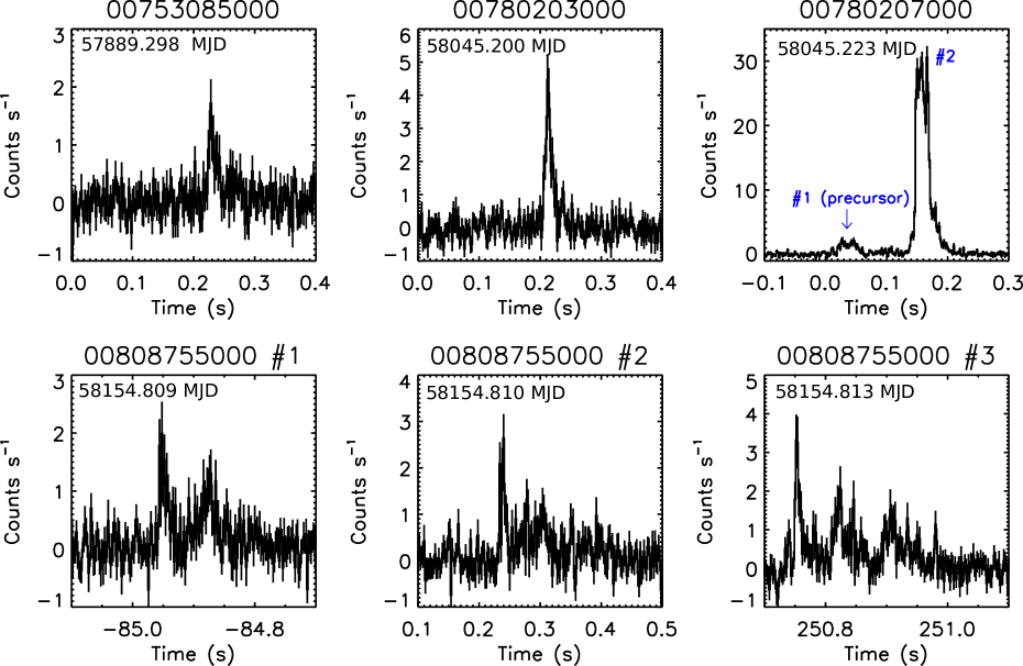
Figure 1: Light curves of the bright bursts detected from CXOU J164710.2–455216 with Swift BAT (as indicated in each panel). The energy range is 15 – 150 keV, the bin size 2 ms and the time is counted from the trigger time of each data set.

2.2 Chandra

Chandra observed CXOU J1647 five times between 2017 May and 2018 April, for a total dead-time corrected exposure time of $\sim$ 75.6 ks. All observations were performed with the Advanced CCD Imaging Spectrometer (ACIS-S; Garmire et al. 2003), set in timed exposure (TE) mode and with faint telemetry format (see Table 2 for a log). The source was always positioned on the back-illuminated S3 chip and 1/8 sub-array was adopted, resulting in a time resolution of $\sim$ 0.44 s. The data were processed following the standard analysis threads with the Chandra Interactive Analysis of Observations software (ciao, version 4.9) and the calibration files caldb 4.7.6.

Source and background photons were collected from a circular region with a radius of 2^′′ and an annular region with inner and outer radii of 4^′′ and 10^′′, centred on the source position. Photon arrival times were converted to the Solar system barycentre using the axbary tool. Source and background spectra with the corresponding response matrices and ancillary files were created with specextract.

2.3 NuSTAR

CXOU J1647 was observed four times with NuSTAR (Harrison et al., 2013); these observations were coordinated with Chandra in order to probe the magnetar emission over a broader energy range thanks to NuSTAR sensitivity to hard X-rays (3 – 79 keV). The two focal plane modules FPMA and FPMB observed the source for a total dead-time corrected exposure time of $\sim$ 91.6 ks and 91.7 ks, respectively.

The data were reprocessed using the script nupipeline of the NuSTAR Data Analysis Software package (nustardas, version 1.8.0) and the calibration files caldb 20171002. We referred the event arrival times to the Solar system reference frame via the tool barycorr and adopting the version 79 of the NuSTAR clock file. Ghost ray contamination is evident in the field of view for all the observations, affecting the detection of the magnetar. The source is detected in the 3 – 8 keV energy band with a S/N of $\sim$ 14. The S/N does not increase when considering a broader energy band, suggesting that the source becomes background dominated above $\sim$ 8 keV. A circle with a 20^′′ radius was used to collect source photons, while background counts were extracted from an annular region with radii of 70^′′ and 130^′′, centred on the source. Using the nuproducts tool, we produced light curves, background-subtracted spectra, instrumental response and auxiliary files for each FPM.

2.4 INTEGRAL

The automatic INTEGRAL Bust Alert System (IBAS, Mereghetti et al., 2003) detected two short bursts in the IBIS/ISGRI data coming from a position compatible with that of CXOU J1647 (note that the IBAS localisation accuracy is 3 arcmin at 90% confidence level). The two events occurred on 2018 February 6 at 07:25:56 UT (trigger ID 8007) and at 12:33:34 UT (trigger ID 8008). An offline search of this data set revealed the presence of a new burst at 00:33:19 UT.

In order to search for additional bursts, we analysed all the available INTEGRAL data collected around the time of the aforementioned detections where the source was serendipitously observed within the field of view of the IBIS/ISGRI instrument (Ubertini et al., 2003; Lebrun et al., 2003). The data were reduced using version 10.2 of the Off-line Scientific Analysis software (OSA) distributed by the ISDC (Courvoisier et al., 2003). The INTEGRAL observations are divided into science windows (SCWs), i.e., pointings with typical durations of $\sim$ 2 – 3 ks. We included in our analysis all SCWs where the source was located within 15 deg from the satellite aim direction, in order to minimise the instrument calibration uncertainties. The data set comprised SCWs in satellite revolutions 1915 and 1916, spanning the time intervals from 2018 February 3 at 14:02 UT to February 4 at 12:14 UT, and from 2018 February 5 at 21:09 UT to February 06 at 12:13 UT. The total exposure time was of 141 ks. We also included all SCWs collected during a dedicated target-of-opportunity observation performed in the direction of the source from 2018 February 7 at 15:04 UT to February 11 at 23:45 UT (total exposure time of 170 ks; satellite revolution 1918). No bursts were found in all these data.

We noticed that the source was observed also at the rim of the IBIS/ISGRI field of view (off-axis angles between 15 and 17 degrees) between 2018 February 5 at 16:52 UT and at 21:09 UT (satellite revolution 1916). Although the instrument calibrations are slightly more uncertain at these higher off-axis angles, two strong bursts were clearly detected. For completeness, we mention that the typical IBIS/ISGRI sensitivity to typical magnetar bursts during these large off-axis observations strongly depends on time, with a median value of 1.7 $\times$ 10^-8 erg s^-1cm^-2 for an integration time scale of 100 ms in the 25 – 80 keV energy range.

Table 1: Log of Swift BAT triggers of CXOU J164710.2–455216 between 2017 May and 2018 February.

Bursta	UTC peak time	S/Nb	$T_{90}$ / total durationc
	(YYYY-MM-DD hh:mm:ss)		(s)
00753085000	2017-05-16 07:09:02.127	8.4	$0.018\pm 0.004$ / 0.021
00780203000	2017-10-19 04:48:48.193	13.7	$0.016\pm 0.004$ / 0.019
00780207000 #1	2017-10-19 05:20:39.695	13.9	$0.031\pm 0.006$ / 0.035
00780207000 #2	2017-10-19 05:20:39.826	55.1	$0.034\pm 0.003$ / 0.060
00808755000 #1	2018-02-05 19:25:46.830	11.1	$0.106\pm 0.018$ / 0.115
00808755000 #2	2018-02-05 19:27:11.968	8.5	$0.008\pm 0.002$ / 0.009
00808755000 #3	2018-02-05 19:31:22.582	19.1	$0.184\pm 0.021$ / 0.206

• The notation #N indicates corresponds to the burst number in a given observation.

• Source signal-to-noise ratio in the 15 – 150 keV image.

• The $T_{90}$ duration is the time during which 90% of the burst counts were accumulated. The total duration is computed by the Bayesian blocks algorithm BATTBLOCKS.

Table 2: Log of the X-ray observations of CXOU J164710.2–455216 between 2017 May 16th and 2018 April 28th.

Obs. ID	Instrument∗	Mid date	Start time (TT)	End time (TT)	Exposure	source net count rate∗∗
		(MJD)	(YYYY-MM-DD hh:mm:ss)		(ks)	(counts s-1)
00753085000	Swift/XRT	57889.303	2017/05/16 07:10:18	2017/05/16 07:21:08	0.6	0.104 $\pm$ 0.013
00030806033	Swift/XRT	57892.970	2017/05/19 02:28:46	2017/05/20 20:04:53	4.7	0.065 $\pm$ 0.004
19135	Chandra/ACIS-S	57898.074	2017/05/25 00:09:57	2017/05/25 03:22:23	9.1	0.223 $\pm$ 0.005
80201050002	NuSTAR/FPMA	57900.298	2017/05/27 01:46:09	2017/05/27 12:31:09	15.7	0.012 $\pm$ 0.001
80201050002	NuSTAR/FPMB	57900.298	2017/05/27 01:46:09	2017/05/27 12:31:09	15.5	0.009 $\pm$ 0.001
00030806034	Swift/XRT	57907.235	2017/06/03 03:50:06	2017/06/03 07:25:54	4.7	0.046 $\pm$ 0.003
00030806035	Swift/XRT	57910.159	2017/06/06 00:38:59	2017/06/06 06:57:53	3.7	0.052 $\pm$ 0.004
00030806036	Swift/XRT	57913.349	2017/06/09 06:31:59	2017/06/09 10:11:54	5.1	0.065 $\pm$ 0.004
19136	Chandra/ACIS-S	57920.141	2017/06/16 01:05:02	2017/06/16 05:42:02	13.7	0.237 $\pm$ 0.004
80201050004	NuSTAR/FPMA	57921.483	2017/06/17 05:11:09	2017/06/17 18:01:09	21.7	0.017 $\pm$ 0.001
80201050004	NuSTAR/FPMB	57921.483	2017/06/17 05:11:09	2017/06/17 18:01:09	21.6	0.014 $\pm$ 0.001
00030806037	Swift/XRT	57922.662	2017/06/18 10:55:52	2017/06/18 20:49:54	3.9	0.055 $\pm$ 0.004
00030806038	Swift/XRT	57934.406	2017/06/30 09:39:21	2017/06/30 09:48:52	0.5	0.048 $\pm$ 0.010
00030806039	Swift/XRT	57937.196	2017/07/03 01:24:26	2017/07/03 08:00:52	3.9	0.052 $\pm$ 0.004
00030806040	Swift/XRT	57943.955	2017/07/09 22:02:26	2017/07/09 23:49:53	1.2	0.047 $\pm$ 0.006
19137	Chandra/ACIS-S	57944.403	2017/07/10 06:37:30	2017/07/10 12:43:59	18.2	0.228 $\pm$ 0.004
80201050006	NuSTAR/FPMA	57948.582	2017/07/14 07:51:09	2017/07/14 20:06:09	22.3	0.015 $\pm$ 0.001
80201050006	NuSTAR/FPMB	57948.582	2017/07/14 07:51:09	2017/07/14 20:06:09	22.8	0.019 $\pm$ 0.001
00030806041	Swift/XRT	57949.561	2017/07/15 10:20:14	2017/07/15 16:34:52	2.3	0.056 $\pm$ 0.005
00030806042	Swift/XRT	57951.496	2017/07/17 02:17:45	2017/07/17 21:29:52	3.8	0.058 $\pm$ 0.004
00030806043	Swift/XRT	57953.801	2017/07/19 14:27:14	2017/07/19 23:59:52	1.5	0.051 $\pm$ 0.006
00030806044	Swift/XRT	57958.322	2017/07/24 01:20:41	2017/07/24 14:05:52	3.7	0.054 $\pm$ 0.004
00030806045	Swift/XRT	57965.468	2017/07/31 03:48:06	2017/07/31 18:38:52	2.9	0.055 $\pm$ 0.004
00030806046d	Swift/XRT	57969.159	2017/08/04 03:46:20	2017/08/04 03:51:54	0.3	0.052 $\pm$ 0.013
00030806047d	Swift/XRT	57974.646	2017/08/09 14:43:54	2017/08/09 16:15:52	0.7	0.057 $\pm$ 0.009
00030806048	Swift/XRT	57978.785	2017/08/13 15:32:41	2017/08/13 22:07:53	3.3	0.047 $\pm$ 0.004
00030806049	Swift/XRT	57981.686	2017/08/16 14:01:52	2017/08/16 18:53:52	1.5	0.057 $\pm$ 0.006
00030806050	Swift/XRT	57993.437	2017/08/27 21:09:16	2017/08/28 23:49:52	0.9	0.052 $\pm$ 0.008
00030806051	Swift/XRT	58006.584	2017/09/10 06:35:31	2017/09/10 21:26:52	5.4	0.050 $\pm$ 0.003
00030806052	Swift/XRT	58020.448	2017/09/24 01:05:51	2017/09/24 20:23:53	1.6	0.056 $\pm$ 0.006
00030806053	Swift/XRT	58023.567	2017/09/27 11:51:57	2017/09/27 15:19:52	3.1	0.052 $\pm$ 0.004
00030806054	Swift/XRT	58033.556	2017/10/07 04:27:26	2017/10/07 22:12:53	4.6	0.043 $\pm$ 0.003
00030806055	Swift/XRT	58038.273	2017/10/12 00:55:33	2017/10/12 12:10:51	4.5	0.050 $\pm$ 0.003
00780203000	Swift/XRT	58045.383	2017/10/19 04:50:42	2017/10/19 13:31:13	13.1	0.078 $\pm$ 0.002
00030806056	Swift/XRT	58046.709	2017/10/20 06:33:41	2017/10/21 03:27:52	4.5	0.066 $\pm$ 0.004
00030806057	Swift/XRT	58138.199	2018/01/19 23:57:40	2018/01/20 09:36:52	3.0	0.045 $\pm$ 0.004
00030806058e	Swift/XRT	58139.335	2018/01/21 07:53:53	2018/01/21 08:09:53	0.9	0.038 $\pm$ 0.006
00030806059e	Swift/XRT	58141.919	2018/01/23 21:58:42	2018/01/23 22:06:53	0.5	0.048 $\pm$ 0.010
00030806060	Swift/XRT	58143.526	2018/01/25 02:59:01	2018/01/25 22:15:53	2.7	0.042 $\pm$ 0.004
00030806061	Swift/XRT	58144.887	2018/01/26 20:22:43	2018/01/26 22:12:52	1.9	0.038 $\pm$ 0.005
00030806062	Swift/XRT	58146.181	2018/01/28 01:04:38	2018/01/28 07:36:52	4.9	0.038 $\pm$ 0.003
00808755000	Swift/XRT	58154.818	2018/02/05 19:28:19	2018/02/05 19:48:21	1.2	0.284 $\pm$ 0.016
00030806064	Swift/XRT (WT)	58156.371	2018/02/07 03:23:29	2018/02/07 14:25:56	2.9	0.138 $\pm$ 0.008
00030806065	Swift/XRT	58160.688	2018/02/11 01:13:41	2018/02/12 07:49:51	5.2	0.068 $\pm$ 0.004
19138f	Chandra/ACIS-S	58174.053	2018/02/24 22:09:30	2018/02/25 04:24:51	18.2	0.286 $\pm$ 0.004
20976f	Chandra/ACIS-S	58174.748	2018/02/25 15:09:14	2018/02/25 20:46:11	16.4	0.278 $\pm$ 0.004
00030806066	Swift/XRT	58174.863	2018/02/25 17:27:40	2018/02/25 23:59:53	4.9	0.069 $\pm$ 0.004
80201050008	NuSTAR/FPMA	58176.276	2018/02/26 19:31:09	2018/02/27 17:46:09	31.9	0.013 $\pm$ 0.001
80201050008	NuSTAR/FPMB	58176.276	2018/02/26 19:31:09	2018/02/27 17:46:09	31.8	0.014 $\pm$ 0.001
00030806069	Swift/XRT	58194.637	2018/03/17 06:34:43	2018/03/17 23:59:54	2.9	0.042 $\pm$ 0.003
00030806070	Swift/XRT	58201.805	2018/03/24 16:43:54	2018/03/24 21:54:53	4.3	0.058 $\pm$ 0.004
00030806071	Swift/XRT	58209.450	2018/04/01 08:21:20	2018/04/01 13:14:52	1.1	0.057 $\pm$ 0.007
00030806072	Swift/XRT	58215.524	2018/04/07 10:59:09	2018/04/07 14:08:51	1.7	0.046 $\pm$ 0.005
00030806073g	Swift/XRT	58219.596	2018/04/11 05:24:09	2018/04/11 23:13:10	0.4	0.064 $\pm$ 0.013
00030806074g	Swift/XRT	58220.956	2018/04/12 22:52:14	2018/04/12 23:03:53	0.7	0.066 $\pm$ 0.009
00030806075	Swift/XRT	58222.190	2018/04/14 03:29:34	2018/04/14 05:37:54	2.1	0.062 $\pm$ 0.005
00030806076	Swift/XRT	58229.605	2018/04/21 12:46:50	2018/04/21 16:15:54	2.2	0.066 $\pm$ 0.005
00030806077	Swift/XRT	58236.834	2018/04/28 18:18:24	2018/04/28 21:45:54	2.7	0.044 $\pm$ 0.004

• Swift XRT operated in PC mode, otherwise specified. Chandra ACIS-S was set in TE mode.

• For Chandra and Swift XRT-PC observations the source net count rate refers to the 0.3 – 10 keV energy band, while for XRT-WT ones to the 1 – 10 keV range. For NuSTAR it corresponds to the 3 – 8 keV energy interval.

• These observations were merged in the spectral analysis.

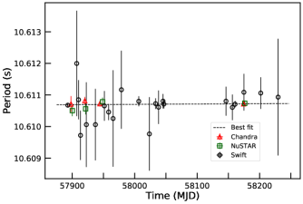
Figure 2: Temporal evolution of the spin period after the Swift BAT trigger on 2017 May 16. Red triangles, green squares and black circles are the measurements from Chandra, NuSTAR and Swift observations, respectively. The dashed line is the linear function which fits the data best (see text for details).

3 Timing analysis

Timing studies for the previous (2006 and 2011) outbursts have been performed by several authors, applying both phase-coherent and non-coherent techniques (Israel et al., 2007; Woods et al., 2011; An et al., 2013; Rodríguez Castillo et al., 2014). In the past, the source exhibited a pulse profile that changed during the outbursts, showing the transition from a simpler morphology to a multi-peaked structure.

For our analysis, we selected events in the 0.3 – 8 keV energy band for Chandra, 0.3 – 10 keV for Swift and 3 – 8 keV for NuSTAR. For the latter, we combined the FPMA and FPMB event files for each observation. First, we tried to build a phase-coherent timing solution starting from the Chandra observation 19138, which was performed about 20 days after the last burst. The Fourier spectrum showed a prominent peak at the spin frequency of CXOU J1647, $\sim$ 10.6 s, and strong harmonic content up to the second harmonic (confirming the pulse profile complex structure close to a bursting activity period). We applied a phase-fitting technique to extend the solution over a longer time interval, but we could not find a solution that aligned all the profiles. We note that a phase-coherent analysis requires to be able to track unambiguously the phase evolution with time of a reference structure in the pulse profile. Due to the different time resolutions, Chandra and NuSTAR pulse profiles showed two peaks, while in most Swift profiles the distinction between the two peaks was not clear, making the choice of a reference structure more complicated.

Therefore, we decided to use a different approach to constrain the average spin down rate. We searched for the spin period in each observation by means of the $Z^{2}_{n}$ test (Buccheri et al., 1983). Given the approximate knowledge of the source period, we run the test in the 10.60 – 10.62 s period range, with the number $n$ of harmonics fixed to 2. We performed Monte Carlo simulations to determine the uncertainty of the best period (for details see Gotthelf et al., 1999). We then fit the best periods as a function of time with a linear function, $P(t)=P_{0}+\dot{P}t$. The best-fitting parameters were $P_{0}$ = 10.608(3) s and $\dot{P}$ = (1 $\pm$ 2) $\times$ 10^-12 s s^-1. The period derivative we measured is consistent with zero, but this does not imply that the source is not spinning down. The data used for the timing analysis do not provide enough sensitivity to measure $\dot{P}$ values as small as those previously obtained for this source. Therefore, we derive the 90% upper limit, 4 $\times$ 10^-12 s s^-1. We note that the obtained upper limit is higher than the estimates reported in previous works (see Table 2 by Rodríguez Castillo et al., 2014). Figure 2 shows the time evolution of the spin period and the best-fitting linear model.

Next, we folded the Chandra and Swift background-subtracted and exposure-corrected light curves on the best period determined in each observation. We studied the shape of the pulse profiles in different energy bands: 0.3 – 8 keV, 0.3 – 2.5 keV (soft band) and 2.5 – 8 keV (hard bard). We chose these energy intervals so as to have comparable photon counting statistics. The Chandra pulse profiles presented a multi-peaked configuration, well modelled by a combination of three sinusoidal functions plus a constant (see Figure 3, left panel), while the Swift profiles could only be reproduced by a constant plus one sine, given the lower statistics and the fact that the time resolution of the PC mode ($\sim$ 2.5 s) is unable to sample accurately the complex profile structure.

Furthermore, we computed the pulsed fraction (defined as the semi-amplitude of the fundamental divided by the average count rate) in the same energy bands and studied its temporal evolution (see Figure 3, right panel). We noted that in all the three energy bands, the pulsed fraction dropped after the last burst and in the last observation it seemed to recover the average pre-outburst value, $\sim$ 48% for the total band, $\sim$ 52% for the soft band and $\sim$ 60% for the hard band.

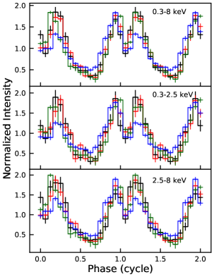
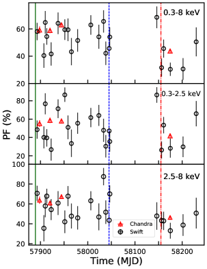
Figure 3: Left: Pulse profiles of CXOU J164710.2–455216 obtained from Chandra observations (black: ID 19135, red: ID 19136, green: ID 19137, blue: merged event file for IDs 19138 and 20976) in different energy bands: 0.3 – 8 keV (top panel); 0.3 – 2.5 keV (middle panel); 2.5 – 8 keV (bottom panel). The pulse profiles are shifted along the horizontal axis for phase alignment and sampled in 16 phase bins. Two cycles are shown for better visualization. Right: Pulsed fraction as a function of time for Chandra (red triangles) and Swift (black circles) pointings in different energy bands: 0.3 – 8 keV (top panel); 0.3 – 2.5 keV (middle panel); 2.5 – 8 keV (bottom panel). The vertical lines denote the epochs of the three BAT triggers: 2017 May 16 at 07:09:02 UT (solid green line), 2017 October 19 at 04:48:48 UT (dashed blue line) and 2018 February 05 at 19:27:11 UT (dash-dotted red line).

4 Spectral analysis

The spectral analysis was performed with the xspec package (version 12.9.1m; Arnaud 1996). Once the best fit was found, the absorbed and unabsorbed fluxes were estimated with the convolution model cflux. For the luminosity quiescent level, we adopted the value 2.6 $\times$ 10³³ erg s^-1, derived by Viganò et al. (2013) with a resonant Compton scattering (RCS) model from the XMM–Newton observation performed on 2006 September 16.

4.1 The BAT burst events

We fit all the burst spectra in the 15 – 150 keV energy range with single-component models typically used for magnetar bursts, such as a power-law (PL), a blackbody (BB) and a bremsstrahlung (BREMSS) component.

The three models provided a statistically equivalent description of the spectra relative to the observations 00753085000, 00780203000, the second and third burst detected in the trigger 00808755000. In Table 3 we report the results relative to the blackbody model. For the first burst in observation 00808755000 and the ‘precursor’ in observation 00780207000, the blackbody model did not give an acceptable fit. The best-fitting values for a power-law model are listed in Table 3. The inclusion of an additional component, in terms of another blackbody, was required for the main event in observation 00780207000 ($F$-test probability of $\sim$ 3 $\times$ 10^-12 for a two-blackbody model).

The most powerful event was the burst that triggered BAT on 2017 October 19 at 05:20:52 UT (trigger 780207); it reached a luminosity of $\sim$ 9 $\times$ 10³⁹ erg s^-1 in the 15 – 150 keV energy band and the ‘precursor’ was about one order of magnitude weaker. The event, which occurred $\sim$ 30 min before (at 04:48:48 UT, trigger 780203), was as intense as the precursor, $L$ $\sim$ 1.5 $\times$ 10³⁹ erg s^-1; the other bursts have a luminosity in the range (5 – 9) $\times$ 10³⁸ erg s^-1.

Table 3: Spectral analysis results for the bursts from CXOU J164710.2–455216 detected by Swift BAT.

Bursta	Model	$kT_{1}$ / $R_{1}$	$kT_{2}$ / $R_{2}$	$\Gamma$	Fluxb	Fluence	$\chi_{\nu}^{2}$ (dof)c
		(keV) / (km)	(keV) / (km)		(10-7 erg s-1cm-2)	(erg cm-2)
00753085000	BB	4.2 $\pm$ 0.8 / 0.5${}^{+0.4}_{-0.1}$			2.5 $\pm$ 0.4	(5.4 $\pm$ 0.8) $\times$ 10-9	1.4 (17)
00780203000	BB	7.1 $\pm$ 0.6 / 0.3 $\pm$ 0.1			9.2 $\pm$ 0.8	(1.7 $\pm$ 0.1) $\times$ 10-8	1.5 (21)
00780207000 #1	PL			2.3 $\pm$ 0.2	7.0 $\pm$ 0.6	(2.4 $\pm$ 0.2) $\times$ 10-8	1.0 (28)
00780207000 #2	2BB	5.1 $\pm$ 0.5 / 0.9 $\pm$ 0.2	12.4 $\pm$ 0.8 / 0.14 $\pm$ 0.02		49.7 $\pm$ 1.1	(2.98 $\pm$ 0.06) $\times$ 10-7	0.7 (35)
00808755000 #1	PL			1.8 $\pm$ 0.2	3.3 $\pm$ 0.4	(3.7 $\pm$ 0.4) $\times$ 10-8	0.6 (28)
00808755000 #2	BB	9.1 $\pm$ 1.6 / 0.2 $\pm$ 0.1			7.5 $\pm$ 1.2	(6.7 $\pm$ 1.1) $\times$ 10-9	0.8 (16)
00808755000 #3	BB	10.2 $\pm$ 0.4 / 0.03 $\pm$ 0.01			2.8 $\pm$ 0.2	(5.8 $\pm$ 0.3) $\times$ 10-9	1.5 (36)

• The notation #N indicates corresponds to the burst number in a given observation.

• In the 15 – 150 keV energy range.

• $\chi_{\nu}^{2}$ is the reduced chi-squared and dof stands for ‘degrees of freedom’.

4.2 The INTEGRAL upper limits

For the observations where bursts were not detected, we estimated a typical sensitivity for IBIS/ISGRI to the typical burst emission at 5$\sigma$ confidence level at 7.9 $\times$ 10^-9 erg s^-1cm^-2, considering an integration time scale of 100 ms in the energy range 25 – 80 keV.

The two bursts observed by INTEGRAL on 2018 February 5 were also independently detected by Swift BAT and Fermi Gamma-Ray Burst Monitor. We report the times and fluences of all bursts detected by IBIS/ISGRI in Table 4, and show the corresponding light curves in Figure 4.

No persistent emission from the source could be detected by IBIS/ISGRI in any of the individual or combined SCWs in revolutions 1915-1918. By stacking all the data together, we obtained an upper limit on the source persistent emission of 3.5 $\times$ 10^-11 erg s^-1cm^-2 in the 20 – 80 keV energy range at 5$\sigma$ confidence level (total effective exposure time of 474.1 ks).

Table 4: Times and fluences in the 25 – 80 keV energy range of the bursts from CXOU J164710.2–455216 detected by the IBIS/ISGRI on-board INTEGRAL during the satellite revolutions 1915-1918.

Trigger time (UTC)	Fluence
(YYYY-MM-DD hh:mm:ss)	(10-8 erg cm-2)
2018-02-05 19:31:22	7.1 $\pm$ 0.8
2018-02-05 20:19:19	7.3 $\pm$ 0.9
2018-02-06 00:33:19	1.7 $\pm$ 0.4
2018-02-06 07:25:56	2.0 $\pm$ 0.5
2018-02-06 12:33:34	2.5 $\pm$ 0.6

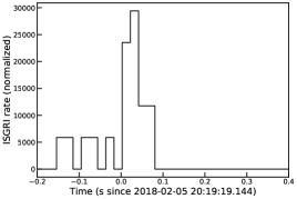
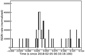
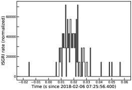
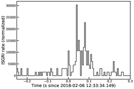
Figure 4: IBIS/ISGRI light curves of all detected bursts during the satellite revolutions 1915-1918. The displayed count rates are corrected for vignetting and refer to the 20 – 80 keV energy band.

4.3 The X-ray monitoring

Because of the different effective areas of the X-ray instruments that translate into different counting statistics, we preferred to fit the Swift XRT data separately from the Chandra and NuSTAR ones. We adopted the model tbabs to describe the photoelectric absorption along the line of sight with photoionization cross-sections from Verner et al. (1996) and chemical abundances from Wilms, Allen & McCray (2000).

First, we present the results of the Swift XRT monitoring campaign. The Swift background-subtracted spectra were rebinned according to a minimum number of counts variable from observation to observation. In most cases, we used less than 10 counts per spectral bin, with the exception of three observations (IDs: 00780203000, 00808755000 and 00030806064) where the larger number of counts was enough to adopt a higher grouping minimum (at least 20 counts per bin). For the Swift spectra, we applied the $W$ statistic (suited for Poisson distributed data with Poisson distributed background). We restricted our spectral modelling to the 0.3 – 10 keV energy band for the PC data, while for the WT mode spectra the energy channels below $\sim$ 1 keV were ignored due to known calibration issues. As a first step, we fit the spectra individually using an absorbed blackbody model (tbabs*bbodyrad). This model provided a good fit to all the observations, except for observations 00780203000 and 00808755000, which are the XRT pointings following the BAT triggers for the latest two bursting events.

We fit these two spectra simultaneously with an absorbed blackbody plus power law model (BB+PL hereafter), forcing the hydrogen column density to be the same across the two data sets. The simultaneous fit yielded $N_{H}$ = (3.4 $\pm$ 0.7) $\times$ 10²² cm^-2. The fit for the observation 00780203000 gave the following parameters: blackbody temperature $kT_{\rm BB}$ = 0.5 $\pm$ 0.1 keV and radius $R_{\rm BB}$ = 1.1${}^{+2.0}_{-0.2}$ km plus a power law with photon index $\Gamma$ = 2.1${}^{+0.6}_{-0.8}$. The other data set (ID: 00808755000) is well described by a blackbody with $kT_{\rm BB}$ = 0.5 $\pm$ 0.1 keV and $R_{\rm BB}$ = 1.8${}^{+1.7}_{-0.5}$ km and a power law with $\Gamma$ = 0.4${}^{+0.9}_{-1.1}$.

In addition to the individual modelling, we fit all the spectra together removing the two above-mentioned ones. The hydrogen column density was constrained to be the same across all the data sets, while the blackbody parameters were left free to vary. The value of $N_{H}$, inferred from the simultaneous fit, was (2.5 $\pm$ 0.1) $\times$ 10²² cm^-2; the temporal evolution of the blackbody temperature and radius is shown in Figure 5, top and middle panels.

The quality of the fit was evaluated performing Monte Carlo simulations; we used the command goodness in xspec to simulate 1000 spectra whose parameters are drawn from Gaussian distributions centred on the best-fit values with width equal to the derived 1$\sigma$ uncertainty. The percentage of simulations with the test statistic less than that for the data ranged from 40% to 60%. Figure 5, left panel, shows the spectra for the observations 00753085000 (May 2017), 00780203000 (Oct 2017) and 00808755000 (Feb 2018) with the respective best-fit models and residuals; these observations are the XRT re-pointings after the BAT triggers. In chronological order, the 0.3 – 10 keV unabsorbed fluxes are (9 $\pm$ 1) $\times$ 10^-12, (1.5${}^{+1.7}_{-0.4}$) $\times$ 10^-11 and (4.3${}^{+0.8}_{-0.5}$ ) $\times$ 10^-11 erg s^-1cm^-2, which translate into a luminosity of (1.8 $\pm$ 0.2) $\times$ 10³⁴, (2.8 $\pm$ 0.8) $\times$ 10³⁴ and (7.8 $\pm$ 1.4) $\times$ 10³⁴ erg s^-1. The Feb 2018 event marked the highest enhancement of the X-ray persistent flux among the registered bursting activities, reaching a luminosity a factor $\sim$ 30 higher than in the quiescent level.

The Chandra background-subtracted spectra were grouped using the optimal binning scheme of Kaastra & Bleeker (2016) by means of the ftool ftgrouppha and fitted in the 0.3 – 8 keV energy range, using the $\chi^{2}$ statistic. We merged observations 19138 and 20976, being only one day apart, having similar count rates and because no significant spectral variability was found. We estimated the impact of pile-up with Webpimms and found that its fraction ranges from 3.5% to 4.5% across the different observations. To correct for this effect, we included the multiplicative pile-up model (Davis, 2001), as implemented in xspec, in the spectral fitting procedure. Following ‘The Chandra ABC guide to Pileup’, we allowed the grade migration parameter $\alpha$ to vary and fixed the parameter psffrac equal to 0.95, i.e. we assumed that 95% of events are within the central, piled-up portion of the source point spread function. The parameter $\alpha$ was forced to be the same across the different observations because of the similar count rates. We fit simultaneously the four spectra applying a blackbody corrected by the pile-up model and tying the hydrogen column up across the different observations. The fit yielded a $N_{H}$ = (2.9 $\pm$ 0.1) $\times$ 10²² cm^-2 ($\chi_{\nu}^{2}$ = 1.0 for 284 dof); the other spectral parameters, the fluxes and luminosities are reported in Table 5. Figure 5, right panel, shows the spectra with the best-fit model and the corresponding residuals.

The NuSTAR spectra were rebinned with at least 20 counts per bin. Since the spectrum is background dominated over $\sim$ 8 keV, these data sets are insufficient to characterize properly the hard X-ray emission of CXOU J1647, but can provide a further check for Chandra results. We fit the NuSTAR spectra simultaneously with the Chandra ones acquired at the same epoch; the inclusion of these new observations did not affect the spectral analysis results. Moreover, we verified that the values of the spectral parameters did not show any dependence on the choice of the size for the background region.

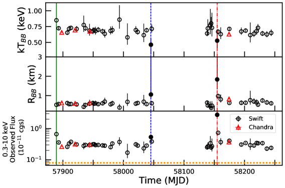
Figure 5: Temporal evolution of the blackbody temperature (top panel) and radius (middle panel) calculated at infinity, assuming a 3.9 kpc distance. In the bottom panel, temporal evolution of the absorbed flux in the 0.3 – 10 keV energy range; the dotted orange line indicates the flux level that the source reached after the 2006 outburst, 8 $\times$ 10^-13 erg s^-1cm^-2 (Coti Zelati et al., 2018). Red triangles are relative to the Chandra pointings and black circles represent Swift XRT observations; the filled circles denote the spectra where a BB+PL model is required. The vertical lines denote the epochs of the three BAT triggers: 2017 May 16 at 07:09:02 UT (solid green line), 2017 October 19 at 04:48:48 UT (dashed blue line) and 2018 February 05 at 19:27:11 UT (dash-dotted red line).

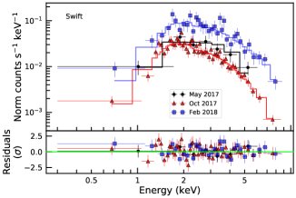
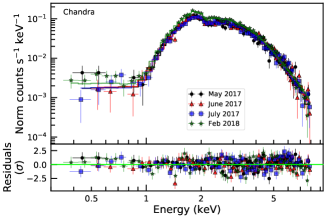
Figure 6: Left: Swift XRT spectra corresponding to the observations following the BAT triggers with the best-fit models (solid line) and the post-fit residuals in units of standard deviations. Right: Chandra spectra fitted with an absorbed blackbody corrected by the pileup model and the residuals with respect to this combined model. For more details see Section 4.3.

Table 5: Spectral analysis results for the Swift XRT (above the line) and Chandra spectra plotted in Figure 5.

ID	$kT$	$R$	$\Gamma$	PL Norma	Fluxabs b	$L_{X}$ b
	(keV)	(km)		10-3	(10-12 erg s-1cm-2)	(1034 erg s-1)
00753085000	0.8 $\pm$ 0.1	0.5 $\pm$ 0.1	–	–	6.6 $\pm$ 1.0	1.8 $\pm$ 0.2
00780203000	0.5 $\pm$ 0.1	1.1${}^{+2.0}_{-0.2}$	2.1${}^{+0.6}_{-0.8}$	2.3 $\pm$ 0.2	5.3 $\pm$ 0.3	2.8 $\pm$ 0.8
00808755000	0.5 $\pm$ 0.1	1.8${}^{+1.7}_{-0.5}$	0.4${}^{+0.9}_{-1.1}$	0.6${}^{+2.9}_{-0.5}$	27.6 $\pm$ 2.6	7.8 $\pm$ 1.4
19135	0.66 $\pm$ 0.01	0.63 $\pm$ 0.03	–	–	2.6 $\pm$ 0.1	0.95 $\pm$ 0.02
19136	0.70 $\pm$ 0.01	0.60 $\pm$ 0.03	–	–	3.21 $\pm$ 0.07	10.9 $\pm$ 0.2
19137	0.68 $\pm$ 0.01	0.62 $\pm$ 0.03	–	–	3.05 $\pm$ 0.06	10.7 $\pm$ 0.2
19138+20976	0.63 $\pm$ 0.01	0.83 $\pm$ 0.02	–	–	3.72 $\pm$ 0.04	14.0 $\pm$ 0.03

• The power law normalization is in units of photons/keV/cm² at 1 keV.

• In the 0.3 – 10 keV energy range.

5 Discussion

We have presented the evolution of the spectral and timing properties of the magnetar CXOU J1647 following its latest outburst activity, which started with the detection of short X-ray bursts in 2017 May. Our monitoring campaign covered $\sim$ 350 days of the outburst evolution, allowing us to characterise accurately the behaviour of the source over a long time span. In the last observation, performed on 2018 April 28, the observed 0.3 – 10 keV flux was (2.4 $\pm$ 0.3) $\times$ 10^-12 erg s^-1cm^-2, about 15 times higher than the historical minimum measured by XMM–Newton in 2006, four days before the first known outburst activation (Muno et al., 2006b).

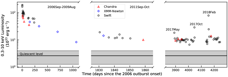
Figure 8: Long-term evolution of the 0.3 – 10 keV luminosity of CXOU J164710.2–455216 from Chandra (red triangles), XMM–Newton (blue diamonds) and Swift (black circles) data acquired between 2006 September and 2018 April. The 2006 outburst onset occurred on 2006 September 21 at 01:34:52 UTC (Krimm et al., 2006). The solid black line denotes the quiescent level (2.6 $\times$ 10³³ erg s^-1) derived with a RCS model by Viganò et al. (2013) from the XMM–Newton observation performed on 2006 September 16. The grey area represents the associated uncertainty.

CXOU J1647 underwent three bursting episodes during this latest activation, entering the small list of magnetars showing recurrent outburst activity, including, e.g., 1E 1048$-$59, 1E 1547$-$5408, SGR 1627$-$41 and 1E 2259$+$586. The emission of short bursts is accompanied by a considerable enhancement of the X-ray persistent flux (see the flux evolution and the long-term light curve in Figure 5, bottom panel, and Figure 8, respectively). To obtain a detailed description of the temporal evolution of the 0.3 – 10 keV luminosity, we modelled the decay pattern following each episode separately using a combination of a constant $L_{q}$ plus one or more exponential functions, depending on the shape of the light curve:

$$L(t)=L_{q}+\sum_{i=1}^{2}A_{i}\times\rm{exp}(-$$t$$/\tau_{i})~{},$$ (1)

where the $e$-folding time $\tau_{i}$ can be considered as an estimate of the decay time scale, similarly to the analysis performed by Coti Zelati et al. (2018).

For the first two flux enhancements in 2017 May and October, the source did not reach the historical quiescent level before the onset of the following event. In these two cases, the constant $L_{q}$ was held fixed to the quiescent value attained after that particular event, i.e. 9.3 $\times$ 10³³ erg s^-1 and 8.4 $\times$ 10³³ erg s^-1 for 2017 May and October events, respectively. The best-fitting model is represented by a simple exponential function in both cases with $e$-folding times $\tau_{May}$ = 2.4${}_{-0.6}^{+1.0}$ d and $\tau_{Oct}$ = 1.3${}_{-0.4}^{+1.1}$ d, which reflect the fast decay at the early stage of these bursting events. For the last outburst episode in 2018 February, the constant was fixed to the quiescent value 2.6 $\times$ 10³³ erg s^-1 (Viganò et al., 2013). In this case, a double-exponential function was required to properly fit the decay with $e$-folding times $\tau_{1,Feb}$ = 0.8${}_{-0.1}^{+0.3}$ d and $\tau_{2,Feb}$ = 167${}_{-39}^{+73}$ d, the latter tracking the long-term decay. We computed the energy released in these outburst episodes by integrating the best-fitting model for the time evolution of the luminosity over the whole duration of the event. The onset of an event is determined by the corresponding BAT triggers. For the first two episodes, the end was set by the beginning of the following event; while for the last one, we extrapolated the epoch of recovery of the quiescent state. During the 2017 May and October events, the source released an energy equal to $\sim$ 1.3 $\times$ 10⁴¹ erg and $\sim$ 8.2 $\times$ 10⁴⁰ erg, respectively. For the latest event, our decay fit predicts that the source will return in quiescence around 2019 October, releasing a total energy of $\sim$ 3.2 $\times$ 10⁴¹ erg. This value is estimated assuming no change in the decay pattern, and should hence be considered only as a rough estimate.

The case of CXOU J1647 is analogous to that of SGR 1627$-$41 and 1E 1547$-$5408, which did not fully recover from their first outbursts in 1998 and 2008, respectively, before resuming a new outburst activity. On the other hand, the case of 1E 1048$-$59 is slightly different since the outbursts seem to be periodic, and the source always returns to its quiescent level before entering a new outburst episode (Archibald et al., 2015).

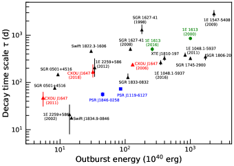
Figure 7: Decay time scale (in term of $e$-folding time) as a function of the total energy released for magnetars showing major outbursts. The triangles refer to the “canonical” magnetars and in red we highlighted the 2006, 2011 and 2018 outbursts of CXOU J164710.2–455216. Blue squares indicate the rotation-powered pulsars with high magnetic fields that showed magnetar-like activity. The green circles denote the two outbursts of 1E 161348–5055, the central source of the supernova remnant RCW 103. Adapted from Coti Zelati et al. (2018).

CXOU J1647 revealed to be a rather prolific magnetar over the past decade, showing two outbursts in 2006 and 2011; the energy released in the 2018 February outburst makes this event the second most powerful recorded so far from this source, with an energy release about a factor of 3 lower than that in 2006 ($E$ $\sim$ 10⁴² erg), and a factor of $\sim$ 5 larger than that measured following the 2011 event ($E$ $\sim$ 6 $\times$ 10⁴⁰ erg). The 2006 and 2011 outbursts are characterized by a decay time scale of $\sim$ 240 d and 50 d, respectively; the time scale of the 2018 event ($\sim$ 170 d) is in between these two values. This result nicely fits in the correlation between the total outburst energy and the corresponding decay time scale found found for magnetars showing major outbursts (Coti Zelati et al., 2018), implying that the longest outbursts are also the most energetic ones (see Figure 7). Moreover, the properties of the 2018 February event also follow the anti-correlation between the quiescent X-ray luminosity and the outburst luminosity increase, as well as the correlation between the energy released during the outburst and the luminosity reached at the outburst onset,for all magnetar outbursts by Coti Zelati et al. (2018) (see Figures 3 and 6 of their work).

During the entire monitoring campaign, excluding the epochs close to the peak of the outbursts, CXOU J1647 showed a thermal spectrum well modelled by an absorbed blackbody. The spectra corresponding to the XRT pointings following the BAT trigger on 2017 October and 2018 February appeared harder, requesting an additional component such as a power law. The spectral hardening in correspondence of bursting activity is an ubiquitous property among magnetars (Esposito et al., 2018). As shown in Figure 5, the inferred blackbody temperature attained a rather high constant value of $\sim$ 0.7 keV over $\sim$ 350 d; the corresponding blackbody radius also settled at a constant value of $\sim$ 0.5 km during the first $\sim$ 160 d. It then increased in correspondence of the bursts, to $\sim$ 1 km and $\sim$ 2 km, and then slowly decaying towards the pre-outburst value.

It is interesting to compare the present results from spectral analysis to those relative to previous outburst episodes from CXOU J1647. Albano et al. (2010) used a three blackbody model, comprising an inner hot cap, a surrounding warm ring and the cooler remaining part of the surface, to reproduce the pulse profiles of CXOU J1647 over a period spanning more than 1000 d, starting from the first XMM–Newton observation after the September 2006 outburst onset. They found that the temperature of the hot cap decreased with time from $0.7$ keV to $0.45$ keV, when it merged with the warm region after $\sim 700$ d. The warm region remained more or less at constant temperature ($\sim 0.45$ keV), with possibly a slight increase at later times. The cooler blackbody was fixed at $0.15$ keV. The area of the hot region shrunk as it cooled, going from an initial $\sim 8\%$ of the entire surface to zero in $\sim 700$ d, while the area of the warm corona increased from $\sim 20\%$ to $\sim 30\%$ of the star surface over the examined time span. The (phase-resolved) spectral analysis by Rodríguez Castillo et al. (2014), relative to the same time span, provides a similar picture, with a hotter spot which cools and shrinks in time and a warm region at roughly constant temperature, although, at variance with the findings of Albano et al. (2010), the area of the latter monotonically decreases in time. Moreover, the two blackbody temperatures reported by Rodríguez Castillo et al. (2014) are somewhat higher.

Regarding the timing properties, the pulse profile shape of CXOU J1647 exhibited quite drastic changes during the previous two outbursts, in 2006 and 2011. From a multi-peaked configuration at the outburst onset, the pulse profile returned to the quiescent single-peaked structure (see Figure 2 by Rodríguez Castillo et al., 2014). In this latest multi-outburst activity period, the pulse profile exhibited two peaks in the Chandra observations (time resolution $\sim$ 0.44 s), confirming the behaviour registered during the past flaring events. In our timing analysis we found an estimate for the period and an upper limit for the period derivative, which are consistent with the results previously reported in literature (Woods et al., 2011; An et al., 2013; Rodríguez Castillo et al., 2014).

The mechanism actually responsible for the heating of the star surface layers in magnetar outbursts is still not well understood. The onset of an active phase is most likely due to a rearrangement of the star external magnetic field, due to the transfer of magnetic helicity from the interior to the magnetosphere, which results in the twist of a bundle of field lines. Currents flowing along the twisted field lines hit the star surface and release heat via Ohmic dissipation. At the same time, the magnetosphere must untwist to maintain the potential drop necessary to accelerate the charges. Beloborodov (2009) discussed the evolution of a twisted magnetosphere and provided a simple estimate for the luminosity released by impinging currents

$$L_{currents}\sim 10^{36}\left(\frac{B}{10^{14}\,\mathrm{G}}\right)\left(\frac{R}{10^{6}\,\mathrm{m}}\right)\left(\frac{\cal V}{10^{9}\,\mathrm{V}}\right)\psi\sin^{4}\theta_{*}\ \mathrm{erg/s}\,,$$ (2)

where $\cal V$ is the potential drop, $\psi$ is the twist angle ($\psi\la\psi_{max}\sim 1\,\mathrm{rad}$) and $\theta_{*}$ is the opening angle of the twisted bundle (which is assumed to be localized around the pole). In the case of CXOU J1647, taking reference values in equation 2, $\psi\sim 1\,\mathrm{rad}$ and $\theta_{*}\la 0.1\,\mathrm{rad}$ (this follows from the measured blackbody radius $\sim 0.1$-$1$ km), the luminosity turns out to be $L_{currents}\la 10^{32}\ \mathrm{erg/s}$. Although non-polar twists can produce a higher luminosity, the previous value is about two orders of magnitude below what observed. This implies that ohmic dissipation of returning currents alone is unlikely to produce the observed thermal flux in CXOU J1647. On the other hand, the predicted evolution timescale of the untwisting magnetosphere,

$$t_{ev}\sim 15\left(\frac{B}{10^{14}\,\mathrm{G}}\right)\left(\frac{R}{10^{6}\,\mathrm{m}}\right)^{2}\left(\frac{\cal V}{10^{9}\,\mathrm{V}}\right)^{-1}\psi\sin^{2}\theta_{*}\ \mathrm{yr}\,,$$ (3)

turns out to be $\sim 1$ month, quite in agreement with observations.

Schematically, the global scenario could then be summarized as follows. Consistently with the expectations of cooling models (Viganò et al., 2013), most of the star has a relatively low temperature (0.1 – 0.2 keV) in its quiescent state. This component could only be detected in a few cases because of the typically high absorption. During the evolution, energy and helicity are transferred from the interior to the magnetosphere until some instability triggers a global magnetic reconnection. The high temperature (0.7 – 1.0 keV), in a very localized component, is likely produced by returning currents of a bundle hitting on the star surface. The energy released in the crust is unlikely to cause such a high surface temperature since the process is not efficient due to neutrino losses and the spread of the heat wave (Pons & Rea, 2012). The origin of the intermediate component (0.3 – 0.5 keV), interpreted as a warm ring around the shrinking central hot spot, is less clear. In most magnetars, this warm component can survive for a long time (years), in most cases being even part of the quiescent emission, and being relatively stable for a decade or more. This does not quite fit in the purely magnetospheric bundle picture, which should be dissipated relatively fast (months). Thus, this intermediate component must be somehow maintained by a continuous energy injection from the interior. Impulsive energy release in the crust has been systematically explored in the literature (Kaminker et al., 2014; Chaikin et al., 2018) and may be part of the solution, although it also has some problems. In particular, multi-D models predict the widening of the warm spot, which is not usually observed. A new interesting idea has recently been proposed by Akgün et al. (2018) who analyzed the coupled evolution of the interior of the star and of a force-free magnetosphere (see also Akgün et al. (2017)). They have estimated the effect that the currents going through the envelope would have on the surface temperature and found that the last $\approx 1$ meter below the surface can be kept at a high temperature in the quasi-stationary regime. Basically, they found that, to close the global current circuit maintaining the twisted magnetosphere on long timescales, currents must go through the low density region between the crust and the exterior, where the electrical resistivity is highest. Releasing energy by Ohmic dissipation in a thin layer of a few meters is very efficient, and the small volume implied requires much less energy to raise the surface temperature to observed values than releasing energy deep in the star crust.

We will continue monitoring the CXOU J1647 with Swift XRT to follow it while recovering its quiescent phase or possibly stabilizing to a new quiescent state, unveil any significant spectral and/or timing evolution, and refine the outburst energetics and decay time scale.

References

- Akgün et al. (2017) Akgün T., Cerdá-Durán P., Miralles J. A., Pons J. A., 2017, MNRAS, 472, 3914
- Akgün et al. (2018) Akgün T., Cerdá-Durán P., Miralles J. A., Pons J. A., 2018, preprint, (arXiv:1807.09021)
- Albano et al. (2010) Albano A., Turolla R., Israel G. L., Zane S., Nobili L., Stella L., 2010, ApJ, 722, 788
- An et al. (2013) An H., Kaspi V. M., Archibald R., Cumming A., 2013, ApJ, 763, 82
- Archibald et al. (2015) Archibald R. F., Kaspi V. M., Ng C.-Y., Scholz P., Beardmore A. P., Gehrels N., Kennea J. A., 2015, ApJ, 800, 33
- Arnaud (1996) Arnaud K. A., 1996, in Jacoby G. H., Barnes J., eds, Astronomical Society of the Pacific Conference Series Vol. 101, Astronomical Data Analysis Software and Systems V. p. 17
- Baumgartner et al. (2011) Baumgartner W. H., et al., 2011, GRB Coordinates Network, Circular Service, 12359, 1 (2011), 12359
- Beloborodov (2009) Beloborodov A. M., 2009, ApJ, 703, 1044
- Borghese et al. (2018) Borghese A., Zelati F. C., Rea N., Esposito P., Mereghetti S., Pintore F., 2018, The Astronomer’s Telegram, 11264
- Buccheri et al. (1983) Buccheri R., et al., 1983, A&A, 128, 245
- Burrows et al. (2005) Burrows D. N., et al., 2005, Space Sci. Rev., 120, 165
- Chaikin et al. (2018) Chaikin E. A., Kaminker A. D., Yakovlev D. G., 2018, preprint, (arXiv:1807.06855)
- Clark et al. (2014) Clark J. S., Ritchie B. W., Najarro F., Langer N., Negueruela I., 2014, A&A, 565, A90
- Coti Zelati et al. (2018) Coti Zelati F., Rea N., Pons J. A., Campana S., Esposito P., 2018, MNRAS, 474, 961
- Courvoisier et al. (2003) Courvoisier T. J.-L., et al., 2003, A&A, 411, L53
- D’Aì et al. (2018) D’Aì A., Evans P. A., Krimm H. A., Kuin N. P. M., Lien A. Y., Page K. L., 2018, GRB Coordinates Network, Circular Service, 21095, (2018)
- Davis (2001) Davis J. E., 2001, ApJ, 562, 575
- Esposito et al. (2018) Esposito P., Rea N., Israel G. L., 2018, preprint, (arXiv:1803.05716)
- Garmire et al. (2003) Garmire G. P., Bautz M. W., Ford P. G., Nousek J. A., Ricker Jr. G. R., 2003, in Truemper J. E., Tananbaum H. D., eds, Proc. SPIEVol. 4851, X-Ray and Gamma-Ray Telescopes and Instruments for Astronomy.. pp 28–44, doi:10.1117/12.461599
- Gotthelf et al. (1999) Gotthelf E. V., Vasisht G., Dotani T., 1999, ApJ, 522, L49
- Harrison et al. (2013) Harrison F. A., et al., 2013, ApJ, 770, 103
- Israel et al. (2007) Israel G. L., Campana S., Dall’Osso S., Muno M. P., Cummings J., Perna R., Stella L., 2007, ApJ, 664, 448
- Israel et al. (2011) Israel G. L., Esposito P., Rea N., 2011, The Astronomer’s Telegram, 3653
- Kaastra & Bleeker (2016) Kaastra J. S., Bleeker J. A. M., 2016, A&A, 587, A151
- Kaminker et al. (2014) Kaminker A. D., Kaurov A. A., Potekhin A. Y., Yakovlev D. G., 2014, MNRAS, 442, 3484
- Kaspi & Beloborodov (2017) Kaspi V. M., Beloborodov A. M., 2017, ARA&A, 55, 261
- Kothes & Dougherty (2007) Kothes R., Dougherty S. M., 2007, A&A, 468, 993
- Krimm et al. (2006) Krimm H., Barthelmy S., Campana S., Cummings J., Israel G., Palmer D., Parsons A., 2006, The Astronomer’s Telegram, 894
- Lebrun et al. (2003) Lebrun F., et al., 2003, A&A, 411, L141
- Li et al. (2016) Li X., Levin Y., Beloborodov A. M., 2016, ApJ, 833, 189
- Malacaria & Roberts (2018) Malacaria C., Roberts O. J., 2018, GRB Coordinates Network, Circular Service, No. 22402, #1-2018 (2018), 22402
- Mazets et al. (1979) Mazets E. P., Golentskii S. V., Ilinskii V. N., Aptekar R. L., Guryan I. A., 1979, Nature, 282, 587
- Mereghetti et al. (2003) Mereghetti S., Götz D., Borkowski J., Walter R., Pedersen H., 2003, A&A, 411, L291
- Muno et al. (2006a) Muno M. P., et al., 2006a, ApJ, 636, L41
- Muno et al. (2006b) Muno M., Gaensler B., Clark J. S., Portegies Zwart S., Pooley D., de Grijs R., Stevens I., Negueruela I., 2006b, The Astronomer’s Telegram, 902
- Olausen & Kaspi (2014) Olausen S. A., Kaspi V. M., 2014, ApJS, 212, 6
- Perna & Pons (2011) Perna R., Pons J. A., 2011, ApJ, 727, L51
- Pons & Perna (2011) Pons J. A., Perna R., 2011, ApJ, 741, 123
- Pons & Rea (2012) Pons J. A., Rea N., 2012, ApJ, 750, L6
- Rea et al. (2016) Rea N., Borghese A., Esposito P., Coti Zelati F., Bachetti M., Israel G. L., De Luca A., 2016, ApJ, 828, L13
- Roberts et al. (2017) Roberts O. J., Hamburg R., Briggs M. S., Connaughton V., Kouveliotou C., Younes G., 2017, GRB Coordinates Network, Circular Service, No. 22027, #1-2018 (2017), 22027
- Rodríguez Castillo et al. (2014) Rodríguez Castillo G. A., Israel G. L., Esposito P., Pons J. A., Rea N., Turolla R., Viganò D., Zane S., 2014, MNRAS, 441, 1305
- Savchenko et al. (2018) Savchenko V., Ferrigno C., Bozzo E., Mereghetti S., Goetz D., Ducci L., 2018, The Astronomer’s Telegram, 11270
- Skinner et al. (2006) Skinner S. L., Perna R., Zhekov S. A., 2006, ApJ, 653, 587
- Thompson & Duncan (1995) Thompson C., Duncan R. C., 1995, MNRAS, 275, 255
- Turolla & Esposito (2013) Turolla R., Esposito P., 2013, International Journal of Modern Physics D, 22, 1330024
- Turolla et al. (2015) Turolla R., Zane S., Watts A. L., 2015, Reports on Progress in Physics, 78, 116901
- Ubertini et al. (2003) Ubertini P., et al., 2003, A&A, 411, L131
- Verner et al. (1996) Verner D. A., Ferland G. J., Korista K. T., Yakovlev D. G., 1996, ApJ, 465, 487
- Viganò et al. (2013) Viganò D., Rea N., Pons J. A., Perna R., Aguilera D. N., Miralles J. A., 2013, MNRAS, 434, 123
- Wilms et al. (2000) Wilms J., Allen A., McCray R., 2000, ApJ, 542, 914
- Woods et al. (2011) Woods P. M., Kaspi V. M., Gavriil F. P., Airhart C., 2011, ApJ, 726, 37
- Younes et al. (2017) Younes G., Kouveliotou C., Gorgogne N., Kennea J., Cenko B., 2017, The Astronomer’s Telegram, 10877